No missing photons for reionization: moderate ionizing photon escape fractions from the FIRE-2 simulations

Abstract

We present the escape fraction of hydrogen ionizing photons ($f_{\rm esc}$) from a sample of 34 high-resolution cosmological zoom-in simulations of galaxies at $z\geq 5$ in the Feedback in Realistic Environments project, post-processed with a Monte Carlo radiative transfer code for ionizing radiation. Our sample consists of 8500 halos in $M_{\rm vir}\sim 10^{8}$–$10^{12}\,M_{\sun}$ ($M_{\ast}\sim 10^{4}$–$10^{10}\,M_{\sun}$) at $z=5$–12. We find the sample average $\langle f_{\rm esc}\rangle$ increases with halo mass for $M_{\rm vir}\sim 10^{8}$–$10^{9.5}\,M_{\sun}$, becomes nearly constant for $10^{9.5}$–$10^{11}\,M_{\sun}$, and decreases at $\gtrsim 10^{11}\,M_{\sun}$. Equivalently, $\langle f_{\rm esc}\rangle$ increases with stellar mass up to $M_{\ast}\sim 10^{8}\,M_{\sun}$ and decreases at higher masses. Even applying single-star stellar population synthesis models, we find a moderate $\langle f_{\rm esc}\rangle\sim 0.2$ for galaxies at $M_{\ast}\sim 10^{8}\,M_{\sun}$. Nearly half of the escaped ionizing photons come from stars 1–3 Myr old and the rest from stars 3–10 Myr old. Binaries only have a modest effect, boosting $\langle f_{\rm esc}\rangle$ by $\sim$25–35% and the number of escaped photons by 60–80%. Most leaked ionizing photons are from vigorously star-forming regions that usually contain a feedback-driven kpc-scale superbubble surrounded by a dense shell. The shell is forming stars while accelerated, so new stars formed earlier in the shell are already inside the shell. Young stars in the bubble and near the edge of the shell can fully ionize some low-column-density paths pre-cleared by feedback, allowing a large fraction of their ionizing photons to escape. The decrease of $\langle f_{\rm esc}\rangle$ at the high-mass end is due to dust attenuation, while at the low-mass end, $\langle f_{\rm esc}\rangle$ decreases owing to inefficient star formation and hence feedback. At fixed mass, $\langle f_{\rm esc}\rangle$ tends to increase with redshift. Although the absolute $\langle f_{\rm esc}\rangle$ does not fully converge with resolution in our simulations, the mass- and redshift-dependence of $\langle f_{\rm esc}\rangle$ is likely robust. Our simulations produce sufficient ionizing photons for cosmic reionization.

1 Introduction

Over the past decade, thanks to a series of deep imaging campaigns carried out with the Hubble Space Telescope (HST) and ground-based facilities, we have obtained relatively robust constraints on the bright-end ($\rm M_{UV}\lesssim-17$) rest-frame ultraviolet luminosity functions (UVLFs) of star-forming galaxies up to $z\sim 8$ (e.g. Bouwens et al., 2015a; Bowler et al., 2015; Finkelstein et al., 2015; Ono et al., 2018) and tentative measurements on the UVLFs at $z\sim 9$–10 (e.g. Oesch et al., 2013, 2014; Bouwens et al., 2016; Stefanon et al., 2017). The Hubble Frontier Fields (HFFs) campaign make it even possible to probe the UVLFs down to $\rm M_{UV}\lesssim-12$ at $z\sim 6$ (e.g. Atek et al., 2015; Atek et al., 2018; Bouwens et al., 2017; Livermore et al., 2017). The upcoming James Webb Space Telescope (JWST; scheduled launch date in March 2021) is expected to remarkably advance our knowledge on the galaxy populations at these redshifts.

These high-redshift star-forming galaxies are thought to be the dominant sources for reionization (e.g. Madau et al. 1999; Faucher-Giguère et al. 2009; Haardt & Madau 2012; Faucher-Giguère 2020; however, see Madau & Haardt 2015), a phase transition of the hydrogen in the intergalactic medium (IGM) from neutral to fully ionized. Cosmic reionization began with the onset of the first generation of stars at $z\sim 20$–30 (e.g. Loeb & Barkana, 2001) and finished by $z\sim 5$ (e.g. Fan et al., 2006a; Becker et al., 2015). The number of ionizing photons emitted from high-redshift galaxies per unit time can be estimated from the observed UVLFs and stellar population synthesis models (e.g. Leitherer et al., 1999; Conroy, 2013; Eldridge et al., 2017). One critical, yet poorly understood, parameter to link high-redshift galaxies to cosmic reionization is the escape fraction of ionizing photons from these galaxies to the IGM ($f_{\rm esc}$).

Models that describe the reionization history from the galaxy populations at $z\geq 5$ need to make assumptions about $f_{\rm esc}$, either a constant $f_{\rm esc}$ for all galaxies or some mass- and redshift-dependent form of $f_{\rm esc}$ (e.g. Finkelstein et al., 2012, 2019; Kuhlen & Faucher-Giguère, 2012; Robertson et al., 2013; Robertson et al., 2015; Bouwens et al., 2015b; Naidu et al., 2020; Yung et al., 2020). Currently available observational constraints on the reionization history, such as the integrated Thomson scattering optical depths (e.g. Planck Collaboration et al., 2016b, 2018), Lyman-$\alpha$ transmission in the Gunn–Peterson trough (e.g. Fan et al., 2006b; Becker et al., 2015), the fraction of Lyman-$\alpha$ emitters (e.g. Stark et al., 2011; Mesinger et al., 2015), and the distribution of Lyman-$\alpha$ equivalent widths (EWs; e.g. Mason et al., 2018, 2019a), suggest $f_{\rm esc}\sim 0.2$, although a robust constraint on $f_{\rm esc}$ and its mass and redshift dependence, cannot yet be achieved.

Direct detection of ionizing or Lyman-continuum (LyC) fluxes from galaxies at $z\gtrsim 5$ is almost impossible. Great efforts have been made to search for rest-frame LyC fluxes from galaxies at $z\sim 0$–4 over the past two decades. Steidel et al. (2001) reported detection of strong LyC flux and inferred high $f_{\rm esc}$ from a stacked spectrum of 29 galaxies at $\langle z\rangle\sim 3.4$ (see also Shapley et al., 2006), but these early studies at $z\gtrsim 3$ likely suffer from foreground contaminations from low-redshift interlopers (e.g. Vanzella et al., 2010; Siana et al., 2015). In the literature, various authors have reported significantly lower $f_{\rm esc}$ (of order 0.01) using galaxy samples from the local Universe to $z\sim 3$ (e.g. Leitherer et al., 1995; Cowie et al., 2009; Bridge et al., 2010; Siana et al., 2010; Boutsia et al., 2011; Leitet et al., 2011, 2013; Grazian et al., 2016, 2017; Rutkowski et al., 2016). Such low $f_{\rm esc}$ is not sufficient for cosmic reionization.

The field has turned around in recent years. Strong LyC leakage has been confirmed from a number of galaxies at $z\sim 0$–4, with inferred $f_{\rm esc}$ from a few per cent to over 50 per cent (e.g. Vanzella et al., 2012, 2016, 2020; Izotov et al., 2016b; Izotov et al., 2016a, 2018; Fletcher et al., 2019; Rivera-Thorsen et al., 2019; Ji et al., 2020). Most of them are compact, extreme starburst galaxies that are thought to be analogs of typical star-forming galaxies in the reionization era. The strong LyC-leaking galaxies share some common properties, such as high $\rm[O\,{\textsc{iii}}]/[O\,{\textsc{ii}}]$ ratios (O32; e.g. Nakajima & Ouchi, 2014; Izotov et al., 2016a), high Lyman-$\alpha$ escape fractions and EWs, double-peak Lyman-$\alpha$ profile with small peak separations (e.g. Verhamme et al., 2015; Verhamme et al., 2017), and weak low-ionization metal absorption lines (e.g. Jaskot & Oey, 2014; Chisholm et al., 2018). There also exist galaxies with comparable O32 ratios and Lyman-$\alpha$ features that do not have detectable LyC fluxes, which are thought to be line-of-sight variations (e.g. Jaskot et al., 2019; Malkan & Malkan, 2019; Nakajima et al., 2020; Izotov et al., 2020). Moderate $f_{\rm esc}\sim 0.1$–0.2 have also been reported recently for considerably large spectroscopic samples of galaxies at $z\sim 3$ after a careful examination of foreground contamination (e.g. Nestor et al., 2013; Steidel et al., 2018). Newly developed cross correlation analysis between star-forming galaxies and IGM transmission at $z\geq 5$ also suggests $f_{\rm esc}\sim 0.1$–0.2 (e.g. Kakiichi et al., 2018; Meyer:2019).

In principle, the common features of strong LyC leakers outlined above may be used as an indirect indicator of $f_{\rm esc}$ from high-redshift galaxies once rest-frame UV-to-optical spectra are accessible at $z\geq 5$ with JWST, potentially offering an independent probe of the contribution of high-redshift galaxies to cosmic reionization. The most important question now is to understand the key physics that governs the escape of ionizing photons, which is also a critical prerequisite for understanding those possible indirect indicators of $f_{\rm esc}$. High-resolution, spatially resolved spectroscopic data of some LyC leakers in the nearby Universe have been obtained recently to address this question (e.g. Keenan et al., 2017; Micheva et al., 2018; Menacho et al., 2019). A comparably detailed theoretical investigation is demanded by these observations.

The escape of ionizing photons involves physics spanning several orders of magnitude in scale. The young stars that produce the majority of the ionizing photons are normally surrounded by dense gas left from the giant molecular clouds (GMCs) in which the stars are formed. Most ionizing photons from the young stars will be absorbed locally before the birth clouds are dispersed (e.g. Kim et al., 2013; Ma et al., 2015; Kimm et al., 2017; Kakiichi & Gronke, 2019; Kim et al., 2019). The time-scale for cloud destruction has to compete with time-scale of massive star evolution, as the ionizing photon budget of a stellar population declines rapidly after the death of the most massive stars in about 3 Myr. Some ionizing photons may also be absorbed by the extended neutral hydrogen in the interstellar medium (ISM) and in the halo before the rest photons escape to the IGM (e.g. Ferrara & Loeb, 2013). Given the complexity, hydrodynamic simulations of galaxy formation form a powerful tool for understanding the escape of ionizing photons.

Early studies using (sub-)kpc-resolution cosmological simulations that cannot properly resolve the ISM structure tend to produce high $f_{\rm esc}$ from tens of per cent to unity (e.g. Razoumov & Sommer-Larsen 2010; Yajima et al. 2011; see also Anderson et al. 2017). Intriguingly, with more detailed treatments of the multi-phase ISM and feedback developed for newer simulations of better resolution, in which the formation and feedback destruction of GMCs start to be resolved, the predicted $f_{\rm esc}$ has been brought down significantly to a few to ten per cent (at least in halos above $M_{\rm vir}\sim 10^{8}\,M_{\sun}$; e.g. Gnedin et al. 2008; Paardekooper et al. 2011, 2015; Kim et al. 2013; Kimm & Cen 2014; Wise et al. 2014; Ma et al. 2015, 2016; Xu et al. 2016; Rosdahl et al. 2018; however, Wise & Cen 2009). Ma et al. (2015) argued in their simulations, ionizing photons from stars younger than 3 Myr are almost entirely consumed by the birth clouds, while there is no longer a sufficiently large ionizing photon budget available from older stars, thereby resulting in $f_{\rm esc}\lesssim 0.05$. Such $f_{\rm esc}$ is at the lower limit of what required for cosmic reionization, hence runaway OB stars (e.g. Conroy & Kratter, 2012; Kimm & Cen, 2014) and binaries (e.g. Ma et al., 2016; Rosdahl et al., 2018) are invoked to provide the ‘missing’ photons, either by making the ionizing photons from young stars escape more easily or producing more ionizing photons after 3 Myr.

Table 1: A list of simulations used in this paper.

Name	$z_{\rm f}$	$M_{\rm halo}$	$M_{\ast}$	$m_{b}$	$m_{\rm DM}$	$\epsilon_{\rm gas}$	$\epsilon_{\rm DM}$	Name	$z_{\rm f}$	$M_{\rm halo}$	$M_{\ast}$	$m_{b}$	$m_{\rm DM}$	$\epsilon_{\rm gas}$	$\epsilon_{\rm DM}$
		[$M_{\sun}$]	[$M_{\sun}$]	[$M_{\sun}$]	[$M_{\sun}$]	[pc]	[pc]			[$M_{\sun}$]	[$M_{\sun}$]	[$M_{\sun}$]	[$M_{\sun}$]	[pc]	[pc]
z5m12b	5	8.73e11	2.55e10	7126.5	3.9e4	0.42	42	z5m10c	5	1.34e10	5.58e7	954.4	5.2e3	0.28	21
z5m12c	5	7.91e11	1.83e10	7126.5	3.9e4	0.42	42	z5m10b	5	1.25e10	3.42e7	954.4	5.2e3	0.28	21
z5m12d	5	5.73e11	1.20e10	7126.5	3.9e4	0.42	42	z5m10a	5	6.60e9	1.48e7	119.3	650.0	0.14	10
z5m12e	5	5.04e11	1.35e10	7126.5	3.9e4	0.42	42	z5m09b	5	3.88e9	2.79e6	119.3	650.0	0.14	10
z5m12a	5	4.51e11	5.36e9	7126.5	3.9e4	0.42	42	z5m09a	5	2.36e9	1.64e6	119.3	650.0	0.14	10
z5m11f	5	3.15e11	4.68e9	7126.5	3.9e4	0.42	42	z7m12a	7	8.91e11	1.66e10	7126.5	3.9e4	0.42	42
z5m11e	5	2.47e11	2.53e9	7126.5	3.9e4	0.42	42	z7m12b	7	6.40e11	1.44e10	7126.5	3.9e4	0.42	42
z5m11g	5	1.98e11	1.86e9	7126.5	3.9e4	0.42	42	z7m12c	7	4.71e11	1.16e10	7126.5	3.9e4	0.42	42
z5m11d	5	1.35e11	1.62e9	7126.5	3.9e4	0.42	42	z7m11a	7	3.32e11	7.17e9	7126.5	3.9e4	0.42	42
z5m11h	5	1.01e11	1.64e9	7126.5	3.9e4	0.42	42	z7m11b	7	2.48e11	2.00e9	7126.5	3.9e4	0.42	42
z5m11c	5	7.57e10	9.45e8	890.8	4.9e3	0.28	21	z7m11c	7	1.63e11	1.81e9	7126.5	3.9e4	0.42	42
z5m11i	5	5.17e10	2.77e8	890.8	4.9e3	0.28	21	z9m12a	9	4.20e11	1.24e10	7126.5	3.9e4	0.42	42
z5m11b	5	4.02e10	1.67e8	890.8	4.9e3	0.28	21	z9m11a	9	2.88e11	3.46e9	7126.5	3.9e4	0.42	42
z5m11a	5	4.16e10	1.22e8	954.4	5.2e3	0.28	21	z9m11b	9	2.23e11	3.49e9	7126.5	3.9e4	0.42	42
z5m10f	5	3.30e10	1.56e8	954.4	5.2e3	0.28	21	z9m11c	9	1.76e11	2.41e9	7126.5	3.9e4	0.42	42
z5m10e	5	2.57e10	3.93e7	954.4	5.2e3	0.28	21	z9m11d	9	1.28e11	1.46e9	7126.5	3.9e4	0.42	42
z5m10d	5	1.87e10	4.81e7	954.4	5.2e3	0.28	21	z9m11e	9	1.16e11	1.49e9	7126.5	3.9e4	0.42	42

• Parameters describing the initial conditions and final galaxy properties of our simulations:

• (1) $z_{\rm f}$: The redshift which the zoom-in region is selected at and the simulation is run to.

• (2) $M_{\rm halo}$ and $M_{\ast}$: Halo mass and total stellar mass within the halo virial radius of the central halo at $z_{\rm f}$.

• (3) $m_{b}$ and $m_{\rm DM}$: Initial baryonic and DM particle mass in the high-resolution region. The masses of DM particles are fixed throughout the simulation. The masses of baryonic (gas and stars) particles are allowed to vary within a factor of two owing to mass loss and mass return due to stellar evolution.

• (4) $\epsilon_{\rm gas}$ and $\epsilon_{\rm DM}$: Plummer-equivalent force softening lengths for gas and DM particles, in comoving units above $z=9$ and physical units thereafter. Force softening for gas is adaptive ($\epsilon_{\rm gas}$ is the minimum softening length). Force softening length for star particles is $\epsilon_{\rm star}=5\epsilon_{\rm gas}$.

More importantly, this suggests that the ‘sub-grid’ models implemented in these simulations have a large impact on the prediction of $f_{\rm esc}$. That being said, this problem should be revisited while simulations are advancing in resolution and sub-grid recipes. Current state-of-the-art cosmological simulations of $z\geq 5$ galaxies are fairly successful in reproducing the observed UVLFs at these redshifts (e.g. Gnedin, 2016; Ocvirk et al., 2016; Ceverino et al., 2017; Ma et al., 2018, 2019; Rosdahl et al., 2018; Wilkins et al., 2018). It is worth emphasizing that large-volume simulations with (sub-)kpc resolution are not well suited for studying $f_{\rm esc}$. Sufficiently detailed treatments of the ISM and feedback physics are mandatory. In this paper, we use a suite of 34 high-resolution cosmological zoom-in simulations of $z\geq 5$ galaxies from the Feedback in Realistic Environments project (FIRE; Hopkins et al., 2018b). These simulations use the FIRE-2 version of the source code gizmo (Hopkins, 2015) that includes an explicit treatment of the multi-phase ISM, star formation, and stellar feedback at the smallest resolved scale.

FIRE-2 is an updated version of the FIRE-1 simulations from Hopkins et al. (2014), including a newly developed hydrodynamic method, a more accurate implementation for mechanical feedback from supernovae (SNe) and stellar winds in Hopkins et al. (2018a), and more subtle differences (see Hopkins et al., 2018b, for details). In this paper, we present a major update to our previous studies on $f_{\rm esc}$ using the FIRE-1 simulations from Ma et al. (2015, 2016). The FIRE simulations are shown to reproduce a broad range of observed galaxy properties at $z\sim 0$–6 (Hopkins et al., 2018b, and references therein). In particular, the simulations studied in this paper produce excellent agreement with the observed galaxy UVLFs at $z\geq 5$ (Ma et al., 2018, 2019).

We post-process these simulations using a three-dimensional Monte Carlo radiative transfer (MCRT) code for ionizing radiation to calculate $f_{\rm esc}$ from 8500 relatively well-resolved galaxies at $z\sim 5$–12 spanning halo masses $M_{\rm vir}\sim 10^{8}$–$10^{12}\,M_{\sun}$ and stellar masses $M_{\ast}\sim 10^{4}$–$10^{10}\,M_{\sun}$. We also investigate the dependence of $f_{\rm esc}$ on galaxy mass and redshift in our simulated sample. Our results provide an essential complement to previous studies from other groups that found a decreasing $f_{\rm esc}$ with halo mass in $M_{\rm vir}\sim 10^{6}$–$10^{9}\,M_{\sun}$ (e.g. Wise et al., 2014; Paardekooper et al., 2015; Xu et al., 2016) by extending the mass-dependence of $f_{\rm esc}$ to higher masses. It is also a key ingredient for modeling the reionization history as reviewed above (e.g. Finkelstein et al., 2019; Yung et al., 2020).

We caution that the prediction of $f_{\rm esc}$ is sensitive to the resolution and sub-grid models adopted in our simulations. Therefore, in this paper, we will mainly focus on the qualitative behaviors rather than the quantitative details of $f_{\rm esc}$. We argue that this caveat may also apply to other studies on $f_{\rm esc}$ using hydrodynamic simulations. In fact, our results of $f_{\rm esc}$ do not yet fully converge with resolution. In Section 2.1, we describe our simulation sample and the ISM, star formation, and stellar feedback model adopted in our simulations. We introduce the MCRT code for our post-processing calculations in Section 2.2. Section 3 presents $f_{\rm esc}$ for our simulations, the mass- and redshift-dependence of $f_{\rm esc}$, and the effects of dust attenuation and binary stars on $f_{\rm esc}$. In Section 4, we investigate the most critical physics that governs the escape of ionizing photons. We discuss our results in Section 5 and conclude in Section 6. Throughout this paper, we define $f_{\rm esc}$ of a galaxy as the absolute fraction of ionizing photons that escape the halo virial radius.

We adopt a standard flat $\Lambda$CDM cosmology with Planck 2015 cosmological parameters $H_{0}=68{\rm\,km\,s^{-1}\,Mpc^{-1}}$, $\Omega_{\Lambda}=0.69$, $\Omega_{m}=1-\Omega_{\Lambda}=0.31$, $\Omega_{b}=0.048$, $\sigma_{8}=0.82$, and $n=0.97$ (Planck Collaboration et al., 2016a). We use a Kroupa (2002) initial mass function (IMF) from 0.1–$100\,M_{\sun}$, with IMF slopes of $-1.30$ from 0.1–$0.5\,M_{\sun}$ and $-2.35$ from 0.5–$100\,M_{\sun}$.

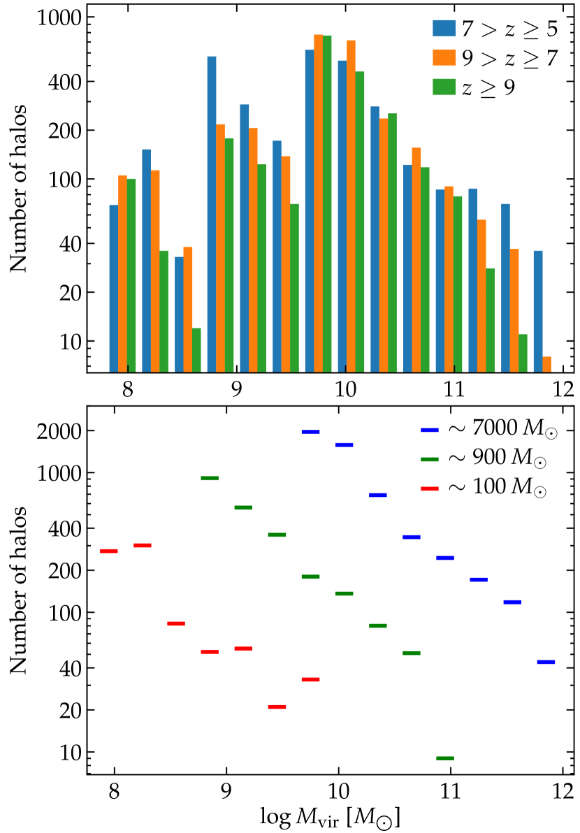
Figure 1: Number of halo snapshots for every 0.3 dex from $M_{\rm halo}=10^{7.8}$–$10^{12}\,M_{\sun}$ in our simulated sample. In the top panel, we divide our sample into three redshift bins regardless of mass resolution. In the bottom panel, we show the sample size at three mass resolution but at all redshift.

2 Method

2.1 The simulations

This work uses a suite of 34 cosmological zoom-in simulations at $z\geq 5$, which we summarize in Table 1. The sample is nearly identical to that presented in Ma et al. (2019), except that simulations z5m10a, z5m11c, and z5m11i are re-run from the same initial conditions using 8 times higher mass resolution. The higher-resolution simulations of z5m10a and z5m11c have been first presented in Ma et al. (2020).

The zoom-in regions are centered around halos chosen at desired mass and redshift from a set of dark matter (DM)-only cosmological boxes. The multi-scale cosmological zoom-in initial conditions are generated at $z=99$ using the music code (Hahn & Abel, 2011) following the method from Oñorbe et al. (2014). We ensure no contamination from low-resolution particles within $2R_{\rm vir}$ of the central halo, and less than 1% contamination by mass within $3R_{\rm vir}$. 22 zoom-in regions are selected from a $(30\,h^{-1}{\rm Mpc})^{3}$ box run to $z=5$ around halos in $M_{\rm halo}\sim 10^{9.5}$–$10^{12}\,M_{\sun}$, 6 others are selected from a $(120\,h^{-1}\,{\rm Mpc})^{3}$ box run to $z=7$, and the rest 6 from an independent box of the same size run to $z=9$. They are centered on halos from $M_{\rm halo}\sim 10^{11}$–$10^{12}\,M_{\sun}$ at $z=7$ and $z=9$, respectively.

The initial mass for baryonic particles (gas and stars) is $m_{b}\sim 100$, 900, or $7000\,M_{\sun}$, and high-resolution DM particles $m_{\rm DM}\sim 650$–$4\times 10^{4}\,M_{\sun}$ in our simulations. Force softening for gas particles is adaptive, with a minimum Plummer-equivalent force softening length $\epsilon_{\rm gas}=0.14$–$0.42\,{\rm pc}$. Force softening lengths for star particles and high-resolution DM particles are fixed at $\epsilon_{\rm star}=5\epsilon_{\rm gas}=0.7$–2.1 pc and $\epsilon_{\rm DM}=10$–42 pc, respectively. The softening lengths are in comoving units at $z>9$ and in physical units thereafter. In Table 1, we provide the final redshift, mass resolution, force softening lengths, final halo mass, and stellar mass for all 34 zoom-in simulations analyzed in this paper.

Figure 2: Number of galaxies for every 0.5 dex in stellar mass from $M_{\ast}=10^{3.75}$–$10^{10.25}\,M_{\sun}$ in our simulation sample. We show the sample size for the three resolution levels but at all redshift.

All simulation are run using an identical version of the code gizmo (Hopkins, 2015) in the meshless finite-mass (MFM) mode with the FIRE-2 models of the multi-phase ISM, star formation, and stellar feedback (Hopkins et al., 2018b), which we briefly summarize below. Gas follows an ionized+atomic+molecular cooling curve in 10–$10^{10}$ K, including metallicity-dependent fine-structure and molecular cooling at low temperatures and high-temperature metal-line cooling for 11 separately tracked species (H, He, C, N, O, Ne, Mg, Si, S, Ca, and Fe). At each timestep, the ionization states and cooling rates for H and He are computed following Katz et al. (1996) and cooling rates from heavier elements are calculated from a compilation of cloudy runs (Ferland et al., 2013), where we apply a uniform, redshift-dependent ionizing background from Faucher-Giguère et al. (2009) and an approximate model for H ii regions generated by local sources. Gas self-shielding is accounted for with a local Jeans-length approximation.

Star formation is allowed only in dense, molecular and locally self-gravitating regions with hydrogen number density above $n_{\rm th}=1000\,{\rm cm}^{-3}$ at 100 per cent efficiency per local free-fall time ($\dot{\rho}_{\ast}=\epsilon\rho/t_{\rm ff}$, where $\epsilon=1$ by default; see Hopkins et al., 2013). Every star particle is regarded as a stellar population with known mass, age, and metallicity assuming a Kroupa (2002) IMF from 0.1–$100\,M_{\sun}$. The simulations account for the following feedback mechanisms: (i) local and long-range radiation pressure, (ii) photoionization and photoelectric heating, and (iii) energy, momentum, mass, and metal injections from SNe and stellar winds. The luminosities, mass loss rates, and Type-II SN rates for each star particle are obtained from starburst99 (Leitherer et al., 1999), and Type-Ia SN rates from Mannucci et al. (2006). These simulations include a sub-resolution turbulent metal diffusion model described in Su et al. (2017) and Escala et al. (2018). We do not consider primordial chemistry nor Pop iii star formation, but adopt an initial metallicity floor of $Z=10^{-4}\,Z_{\sun}$. We emphasize that our photoionization feedback only includes a very approximate model for H ii regions: from each newly formed star particle, we move radially outwards and ionize neutral gas particles one by one until the the ionizing photon budget of the star is exhausted; ionized gas is set to $10^{4}$ K and photoelectric heating is included following the rates from Wolfire et al. (2003). Hopkins et al. (2020) show that this approximate model does not make a big difference on galaxy-scale dynamics compared to more accurate radiation-hydrodynamic method even in halos down to $M_{\rm halo}\sim$ $10^{9}\,M_{\sun}$ by $z=0$. In this work, we use post-processing MCRT calculations (Section 2.2) to obtain more accurate solutions of the ionization states, but we caution that the dynamical effect of photoionization feedback may not be correctly captured.

We use the Amiga’s halo finder (ahf; Knollmann & Knebe, 2009) to identify halos and galaxies in the snapshots, applying the redshift-dependent virial parameter from Bryan & Norman (1998). There are more than one halo in each zoom-in region. In this work, we restrict our analysis to halos that have zero contamination from low-resolution particles within $R_{\rm vir}$ and contain more than $10^{5}$ DM particles to ensure sufficient resolution for calculating $f_{\rm esc}$. We also do not consider subhalos independently in this work. We utilize all snapshots we saved in our analysis and treat the same halo across different snapshots as different ‘galaxies’. The typical time separation is $\sim 16$ Myr between two consecutive snapshots. This is to account for short-time-scale variabilities of galaxy properties due to bursty star formation (e.g. Ma et al., 2018) and to maximize the statistical power of our simulation sample. Fig. 1 shows the number of halo snapshots in our simulated sample in bins of 0.3 dex in halo mass from $M_{\rm halo}=10^{7.8}$–$10^{12}\,M_{\sun}$ for three redshift bins ($5\leq z<7$, $7\leq z<9$, and $z\geq 9$) at any resolution (top) and for the three mass resolution levels at all redshifts (bottom). Fig. 2 shows the number of snapshots in bins of 0.5 dex in stellar mass from $M_{\ast}=10^{3.75}$–$10^{10.25}\,M_{\sun}$ for the three resolution levels at all redshifts. There are 8500 ‘galaxies’ in total from $z=5$–12 in our simulated sample.

2.2 Monte Carlo radiative transfer of ionizing radiation

We post-process every galaxy snapshot using a three-dimensional MCRT code to solve ionizing photon transport and ionization balance, from which we obtain $f_{\rm esc}$ as a product. For every simulated galaxy, we map all gas particles within $R_{\rm vir}$ onto an octree grid: we first deposit all particles in a cubic root cell of side length equal to $2R_{\rm vir}$ and adaptively divide a parent cell into eight child cells until no leaf cell contains more than 2 gas particles. The minimum cell size in the densest region is usually less than 1 pc even for the most massive galaxies in our sample. All physical quantities of a cell are evaluated using 32 nearest gas particles smoothed by a cubic spline kernel. We include all star particles within $R_{\rm vir}$ in our calculations. The hydrogen ionizing photon production rate of each star particle is computed from its age and metallicity using the Binary Population and Spectral Synthesis (BPASS) model (v2.2.1; Eldridge et al., 2017). We consider both the single-star and binary models and will compare the results in Section 3.2.3. The BPASS single-star models are very close to the starburst99 models adopted in our simulations for stellar feedback. We only consider binary models in post- processing, but we do not expect them to have a large effect on the feedback (e.g. Hopkins et al., 2018b).

Table 2: Three choices of stellar population and dust models we adopt for our Monte Carlo radiative transfer calculations.

Model	Stellar population modela	Dust modelb
I (default)	single-star	default
II	binary	default
III	single-star	no dust

• ^a Both single-star and binary models are taken from the BPASS models (version 2.2.1).

• ^bOur default dust model adopts a constant dust-to-metal ratio of 0.4 in gas below $10^{6}$ K (no dust at higher temperatures) with opacity $3\times 10^{5}\,{\rm cm}^{2}\,{\rm g}^{-1}$ and albedo 0.277 at the Lyman limit.

The structure of our MCRT code is similar to those described in previous works (e.g. Fumagalli et al., 2011; Ma et al., 2015; Smith et al., 2019). A total number of 1–$2.4\times 10^{8}$ photon packets are emitted isotropically from the location of star particles, sampled by their ionizing photon emissivity. The same number of photon packets are sent from domain boundary inwards to create an isotropic, uniform ionizing field with intensity given by Faucher-Giguère et al. (2009). Each photon packet is propagated until it escapes the domain, or is absorbed. The number of photon packets we use is sufficiently large such that it does not affect our results on $f_{\rm esc}$. These photon packets are used to construct the ionization radiation field in the domain.

A photon packet may be absorbed by a neutral hydrogen atom with photoionization cross section from Verner et al. (1996). It may also be absorbed or scattered by dust grains. In our default calculations, we assume (a) 40% of the metals are locked in dust grains in gas below $10^{6}$ K while no dust in gas at higher temperature (e.g. Dwek, 1998) and (b) the dust follows the Small Magellanic Cloud (SMC) grain-size distribution from Weingartner & Draine (2001), which gives a dust opacity $3\times 10^{5}\,{\rm cm}^{2}\,{\rm g}^{-1}$ and an albedo 0.277 at the Lyman limit. When the transport of all photon packets is done, we solve the ionization state for each cell assuming ionization equilibrium, where we adopt the temperature-dependent collisional ionization rates in Jefferies (1968) and recombination rates in Verner & Ferland (1996). We take the gas temperatures in the simulations to compute these rates, since the simulations also take into account other heating sources (e.g. shocks) besides photo-heating. We iteratively transport photon packets and update the ionization states to reach convergence. We find 10 iterations sufficient for our purpose. In this paper, we consider three combinations of stellar population and dust models in our MCRT calculations as listed in Table 2. We focus on results from Model I, where we use single-star model and our default dust models, unless stated otherwise. We compare the results between these models in Section 3.2.

In previous works, we have shown that our default dust model produces reasonable attenuation in the UV, bright-end UVLFs, and the relation between infrared excess and UV slope (i.e. the IRX–$\beta$ relation; see Ma et al. 2018, section 6 and Ma et al. 2019). Nonetheless, this treatment is still simplistic and a detailed investigation on dust grain physics is beyond the scope of this paper. We consider a model where dust is ignored completely (Model III in Table 2) and compare the results with those in our default model to bracket the effect of dust on $f_{\rm esc}$ (Section 3.2.2).

3 The escape fraction of ionizing photons

In this section, we present the ionizing photon escape fraction, $f_{\rm esc}$, for our simulated sample, its correlation with galaxy mass and redshift, and the effects of stellar population and dust on these results. We reiterate the fact that the $f_{\rm esc}$ of a galaxy is defined as the absolute fraction of ionizing photons that escape the virial radius of the halo. We investigate the key physics that governs the escape of ionizing photons in Section 4.

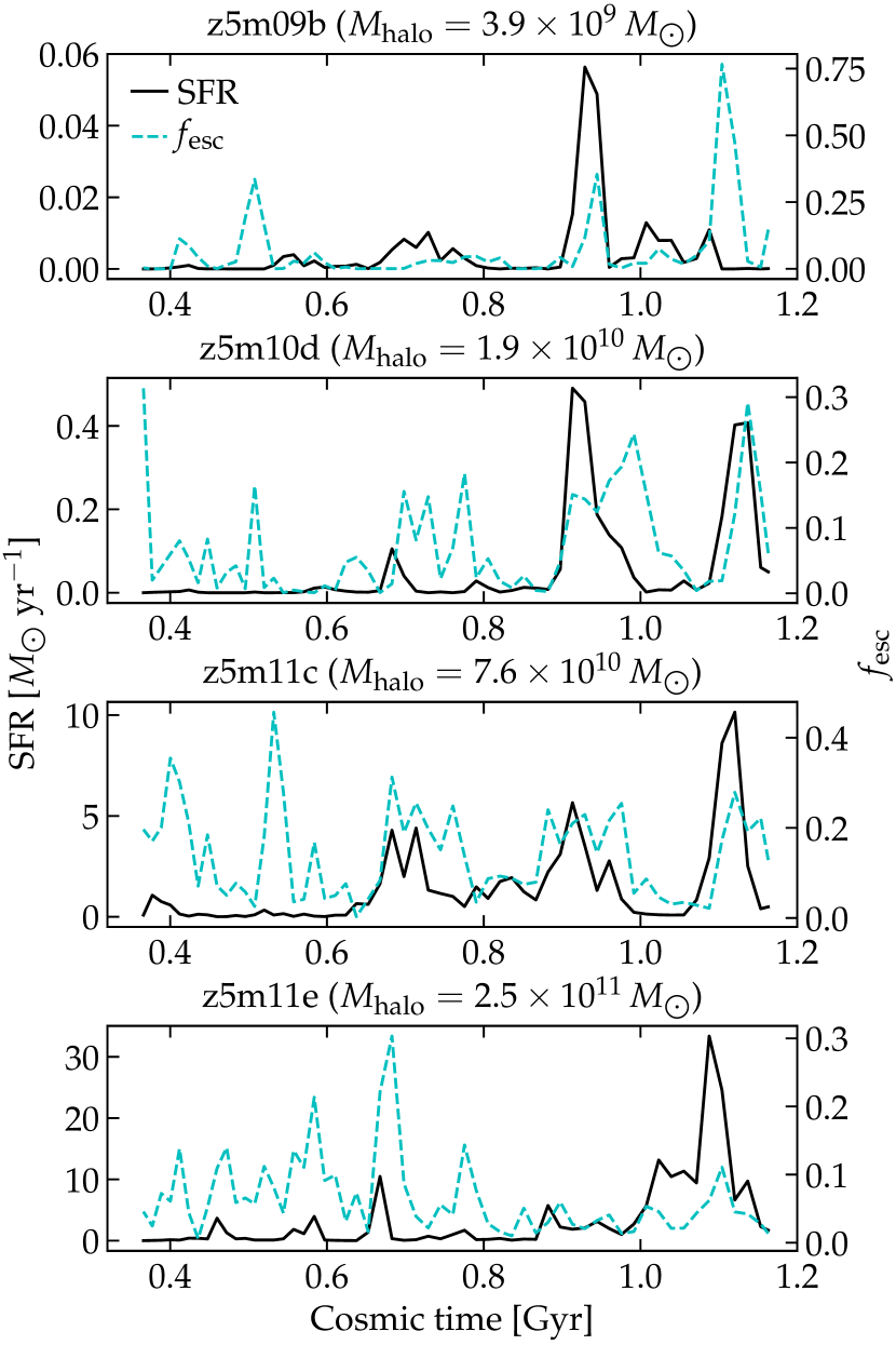
Figure 3: The star formation rate (SFR; black solid lines) and instantaneous escape fraction ($f_{\rm esc}$; cyan dashed lines) for four galaxies in our simulations, using single-star and our default dust models. Both the SFR and $f_{\rm esc}$ show large variabilities on short time-scales. There is usually a time lag between the rising of $f_{\rm esc}$ and the rising of SFR at the beginning of a starburst, as it takes some time for feedback to clear the sightlines where ionizing photons can escape. Note that a galaxy may have high $f_{\rm esc}$ but low SFR at certain epochs, meaning that it is not leaking a large number of ionizing photons.

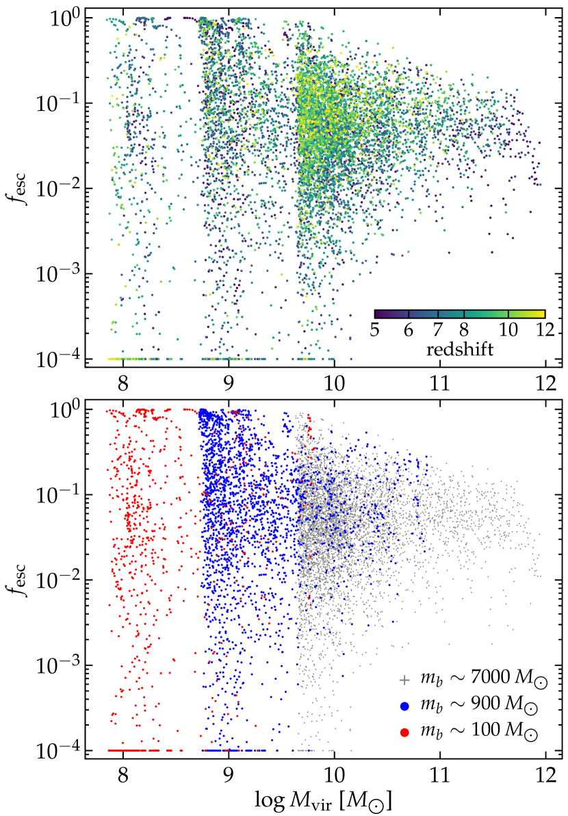
Figure 4: The $f_{\rm esc}$–$M_{\rm vir}$ relation (using single-star and default dust model). Each point shows a halo snapshot in our simulated sample. In the top panel,
the points are color-coded by redshift. In the bottom panel, the colors represent the mass resolution of the simulation. The instantaneous $f_{\rm esc}$ has a large scatter (2–4 dex) at a given $M_{\rm vir}$. Again, a high $f_{\rm esc}$ does not necessarily mean the galaxy is leaking a large number of ionizing photons, as the SFR may be low at these epochs.

3.1 The instantaneous escape fraction

Fig. 3 shows the star formation rate (SFR; black solid lines) and $f_{\rm esc}$ (cyan dashed lines) as a function of cosmic time for four examples in our sample: the central halos in z5m09b, z5m10d, z5m11c, and z5m11e, with halo mass spanning in $M_{\rm vir}\sim 10^{9.6}$–$10^{11.5}\,M_{\sun}$ by $z=5$. For each simulation, we show the 57 epochs from $z=12$ to 5 at which we saved a snapshot. Both $f_{\rm esc}$ and the SFR show large time variabilities, with $f_{\rm esc}$ changing from nearly zero to order unity (e.g. $\gtrsim 20\%$) on short time-scales. There is usually a time delay between the rising of $f_{\rm esc}$ and the rising of SFR when a starburst begins (e.g. z5m09b at $t\sim 0.9$ Gyr, z5m10d, and z5m11c at $t\sim 1.1$ Gyr). This has been reported in our previous works (e.g. Ma et al., 2015; Smith et al., 2019) and is because it takes a few Myrs for stellar feedback to clear some sightlines before a considerable fraction of the ionizing photons are allowed to escape. In Section 4.1, we further show how feedback determines the escape of ionizing photons.

Fig. 4 shows the relation between $f_{\rm esc}$ and halo mass $M_{\rm vir}$ for our simulated sample. Each point represents a halo snapshot. In the top panel, the color shows the redshift of the snapshot, while in the bottom panel, we separate the points by the mass resolution we use for each simulation as $m_{b}\sim 7000\,M_{\sun}$ (grey), $900\,M_{\sun}$ (blue), and $100\,M_{\sun}$ (red). If a galaxy has $f_{\rm esc}<10^{-4}$, we plot it at $10^{-4}$. At a given $M_{\rm vir}$, $f_{\rm esc}$ shows a large scatter, spanning from less than $10^{-4}$ to unity. We caution that a galaxy with instantaneous $f_{\rm esc}\sim 1$ does not mean it is leaking a large number of ionizing photons, as seen from Fig. 3 that there are some epochs at which $f_{\rm esc}$ is high but the SFR is very low. This happens more often in low-mass halos (or at early times), likely because feedback has blown out most of the gas at such epochs. Galaxies at different redshift, or run with different resolution, overlap largely on the $f_{\rm esc}$–$M_{\rm vir}$ plane. At $\log M_{\rm vir}\gtrsim 10$, the smaller scatter is likely due to weaker bursty star formation at higher masses (e.g. Hopkins et al., 2014; Kimm & Cen, 2014). The scatter in this relation is too large to reveal any significant correlation of $f_{\rm esc}$ with $M_{\rm vir}$ or redshift, or the robustness of our results to mass resolution. We address these questions by studying the sample averaged $\langle f_{\rm esc}\rangle$ in Section 3.2.

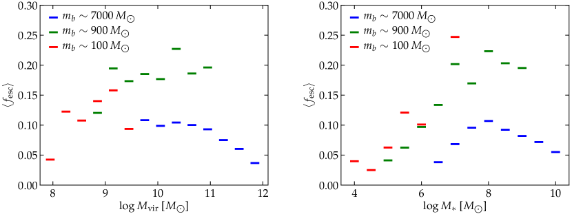
Figure 5: The sample average $\langle f_{\rm esc}\rangle$ as a function of $M_{\rm vir}$ (left) and $M_{\ast}$ (right) (using single-star and default dust model). $\langle f_{\rm esc}\rangle$ is defined as the $Q_{\rm ion}$-weighted instantaneous $f_{\rm esc}$ over all snapshots at all redshifts in a given halo/stellar mass bin. The blue, green, and red bars represent simulations at $m_{b}\sim 7000$, 900, and $100\,M_{\sun}$ resolution. Our results do not fully converge with resolution. Simulations at $m_{b}\sim 7000\,M_{\sun}$ resolution tend to produce lower $\langle f_{\rm esc}\rangle$ than simulations at $m_{b}\sim 900\,M_{\sun}$ or better resolution. $\langle f_{\rm esc}\rangle$ increases with $M_{\rm vir}$ in $\log M_{\rm vir}\sim 8$–9.5, becomes nearly independent of $M_{\rm vir}$ in $\log M_{\rm vir}\sim 9.5$–11, and decreases with $M_{\rm vir}$ above $\log M_{\rm vir}\sim 11$. $\langle f_{\rm esc}\rangle$ increases with $M_{\ast}$ up to $\log M_{\ast}\sim 8$ and decreases with $M_{\ast}$ at higher masses. The decrease of $f_{\rm esc}$ at the high- and low-mass end is due to increasingly strong dust attenuation (cf. Fig. 6 and Section 3.2.2) and inefficient star formation and feedback (cf. Figs. 9–11 and Section 4.4), respectively. It is worth noting that the compromise between these two effects results in the apparent independence of $\langle f_{\rm esc}\rangle$ on $M_{\rm vir}$ in $\log M_{\rm vir}\sim 9.5$–11.

3.2 The average escape fraction

3.2.1 Correlations with galaxy mass

We divide our sample into 14 equal-width bins in logarithmic halo mass from $\log M_{\rm vir}=7.8$–12, with a bin width of 0.3 dex. For each bin, we compute the average escape fraction over all halo snapshots in that bin, $\langle f_{\rm esc}\rangle=\sum_{i}Q_{{\rm esc},\,i}/\sum_{i}Q_{{\rm ion},\,i}=\sum_{i}f_{{\rm esc},\,i}\,Q_{{\rm ion},\,i}/\sum_{i}Q_{{\rm ion},\,i}$, where $Q_{{\rm ion},\,i}$ and $Q_{{\rm esc},\,i}$ are the number of ionizing photons emitted and escaped per unit time, and $f_{{\rm esc},\,i}$ is the escape fraction of the $i^{\rm th}$ galaxy in the bin. In the left panel of Fig. 5, we show the correlation between $\langle f_{\rm esc}\rangle$ and halo mass $M_{\rm vir}$. The color separates simulations run with different resolution (blue: $m_{b}\sim 7000\,M_{\sun}$, green: $900\,M_{\sun}$, and red: $100\,M_{\sun}$). Here we average over galaxies at all redshifts in a given mass bin, but we study redshift dependence later in Section 3.2.4. Note that certain bins do not have a large number of galaxies ($\lesssim 100$, see Fig. 1), which may introduce noise to our results.

Our results on $\langle f_{\rm esc}\rangle$ do not yet fully converge with resolution. Simulations at $7000\,M_{\sun}$ resolution tend to produce systematically lower $\langle f_{\rm esc}\rangle$ than those at $900\,M_{\sun}$ resolution or better, while we do not find significant differences between simulations at $900\,M_{\sun}$ and $100\,M_{\sun}$ resolution. Now we focus on the qualitative trend between $\langle f_{\rm esc}\rangle$ and $M_{\rm vir}$. For intermediate halo mass (i.e. $\log M_{\rm vir}\sim 9.5$–11), $\langle f_{\rm esc}\rangle$ is nearly constant and does not depend strongly on halo mass. This trend is found both for simulations at $7000\,M_{\sun}$ resolution and at $900\,M_{\sun}$ or better resolution, although the absolute value of $\langle f_{\rm esc}\rangle$ differs between the two subsamples. In this halo mass range, $\langle f_{\rm esc}\rangle$ is roughly 0.2 for simulations at $900\,M_{\sun}$ resolution, while $\langle f_{\rm esc}\rangle\sim 0.1$ for those at $7000\,M_{\sun}$ resolution. At the massive end (i.e. above $\log M_{\rm vir}\sim 11$), $\langle f_{\rm esc}\rangle$ decreases with halo mass and drops to 0.03 at $\log M_{\rm vir}\sim 12$. This is due to increasingly important dust attenuation at higher masses (cf. Fig. 6 and Section 3.2.2). Below $\log M_{\rm vir}\sim 9$, $\langle f_{\rm esc}\rangle$ decreases with decreasing halo mass and drops under 0.05 at $\log M_{\rm vir}\sim 8$. We discuss in Section 4.4 that this is likely due to less efficient star formation and stellar feedback in low-mass galaxies in clearing the gas for ionizing photons to escape. We emphasize that the apparent independence of $\langle f_{\rm esc}\rangle$ on $M_{\rm vir}$ from $\log M_{\rm vir}\sim 9.5$–11 is likely a coincidence: we show below in Section 3.2.2 that if there is no dust, $\langle f_{\rm esc}\rangle$ will increase with $M_{\rm vir}$ up to $M_{\rm vir}\sim 10^{11}\,M_{\sun}$ (cf. Fig. 6), and the effect of dust attenuation becomes increasingly strong at higher masses, leading to a nearly constant $\langle f_{\rm esc}\rangle$ at intermediate halo mass.

We also bin our sample in every 0.5 dex in stellar mass into 13 equal-width stellar mass bins from $\log M_{\ast}\sim 3.75$–10.25. We show in the right panel of Fig. 5 the correlation between $\langle f_{\rm esc}\rangle$ and stellar mass, where we average $f_{\rm esc}$ over galaxies at all redshifts in a given stellar mass bin and the color represents the resolution used for our simulations. Again, simulations run at $7000\,M_{\sun}$ resolution produce systematically lower $\langle f_{\rm esc}\rangle$ than those run at $900\,M_{\sun}$ resolution or better, but the qualitative behavior of the $\langle f_{\rm esc}\rangle$–$M_{\ast}$ relation agrees well between the two subsamples. We find that that $\langle f_{\rm esc}\rangle$ increases with stellar mass until $\log M_{\ast}\sim 8$, where $\langle f_{\rm esc}\rangle$ starts to decrease at higher masses. We obtain $\langle f_{\rm esc}\rangle\sim 0.2$ (0.1) for $900\,M_{\sun}$ ($7000\,M_{\sun}$) resolution at $\log M_{\ast}\sim 8$ where $\langle f_{\rm esc}\rangle$ peaks. Similar to what mentioned above, the low $\langle f_{\rm esc}\rangle$ at the high- and low-mass end is due to heavy dust attenuation and inefficient feedback, respectively, which we explicitly show later in this paper.

We reiterate the facts that simulations at $7000\,M_{\sun}$ resolution and those at $900\,M_{\sun}$ or better resolution predict broadly consistent trends between $\langle f_{\rm esc}\rangle$ and $M_{\rm vir}$ ($M_{\ast}$) where the mass overlaps. Also, simulations at $900\,M_{\sun}$ and $100\,M_{\sun}$ resolution predict broadly similar $\langle f_{\rm esc}\rangle$. This suggests that the qualitative trend in the $\langle f_{\rm esc}\rangle$–$M_{\rm vir}$ ($M_{\ast}$) relation from Fig. 5 is likely robust and not an artifact due to the non-trivial selection criteria for our simulated sample.

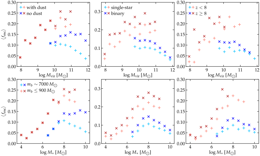
Figure 6: The $\langle f_{\rm esc}\rangle$–$M_{\rm vir}$ (top) and $\langle f_{\rm esc}\rangle$–$M_{\ast}$ (bottom) relation, separated by simulations at $7000\,M_{\sun}$ resolution (blue) and at $900\,M_{\sun}$ resolution or better (red). Left column: $\langle f_{\rm esc}\rangle$ with (light plus signs) and without (dark cross signs) dust attenuation. $\langle f_{\rm esc}\rangle$ increases with halo (stellar) mass up to $\log M_{\rm vir}\sim 11$ ($\log M_{\ast}\sim 8$) and becomes roughly constant at higher masses without dust attenuation, suggesting the decrease of $\langle f_{\rm esc}\rangle$ at the high-mass end in Fig. 5 is due to dust attenuation (Section 3.2.2). Middle column: $\langle f_{\rm esc}\rangle$ calculated using single-star (plus) and binary (cross) stellar population models. Binary models tend to boost $\langle f_{\rm esc}\rangle$ by $\sim 25$–35% in most mass bins, as they predict more ionizing photons for a stellar population after 3 Myr and the extra photons have a higher possibility to escape (cf. Fig. 9 and Section 4.3). Binary stars increase the number of ionizing photons emitted by $\sim 20$–30%, and thus the number of ionizing photons escaped by $\sim 60$–80% (Section 3.2.3). Right column: The dependence of $\langle f_{\rm esc}\rangle$ on redshift. The sample is divided into two redshift bins: $z<8$ (plus) and $z\geq 8$ (cross). Galaxies at higher redshifts tend to have systematically higher $\langle f_{\rm esc}\rangle$ than galaxies at lower redshifts (Section 3.2.4).

3.2.2 The effects of dust attenuation

For every halo above $M_{\rm vir}=10^{10}\,M_{\sun}$ in our simulations, we repeat the MCRT calculations without dust extinction and scattering (‘no dust’, i.e. Model III in Table 2). We expect dust to be subdominant in halos below $M_{\rm vir}=10^{10}\,M_{\sun}$, as they are much less dust-enriched than more massive halos. In the left column of Fig. 6, we compare the $\langle f_{\rm esc}\rangle$–$M_{\rm vir}$ relation (top panel) and the $\langle f_{\rm esc}\rangle$–$M_{\ast}$ relation (bottom panel) with and without dust attenuation. Blue and red symbols represent simulations run at $7000\,M_{\sun}$ resolution and at $900\,M_{\sun}$ or better resolution, respectively. Thereafter, we combine simulations at $900\,M_{\sun}$ and $100\,M_{\sun}$ resolution, given that we do not find a significant difference between the two resolution and our sample does not contain a sufficiently large number of galaxies at $100\,M_{\sun}$ resolution. The light plus and dark cross signs show the results from Model I (with our default dust model) and Model III (without dust attenuation), respectively. Combining the qualitative trend revealed by the two subsamples at $\sim 7000\,M_{\sun}$ and at $\lesssim 900\,M_{\sun}$ resolution, we find that without dust attenuation, $\langle f_{\rm esc}\rangle$ increases with $M_{\rm vir}$ and $M_{\ast}$ until $M_{\rm vir}\sim 10^{11}\,M_{\sun}$ and $M_{\ast}\sim 10^{8}\,M_{\sun}$ to 0.25 (0.15) for simulations at $900\,M_{\sun}$ ($7000\,M_{\sun}$) resolution, and turns nearly constant at the more massive end. This suggests that the seemingly constant $\langle f_{\rm esc}\rangle$ over $\log M_{\rm vir}\sim 9.5$–11 and the decrease of $\langle f_{\rm esc}\rangle$ at the high-mass end ($\log M_{\rm vir}\gtrsim 11$, $\log M_{\ast}\gtrsim 8$) are due to increasingly heavy dust attenuation.

3.2.3 The effects of binary stars

We also repeat our MCRT calculations with the binary stellar population models instead of the single-star models from BPASS (i.e. Model II in Table 2). The binary models include mass transfer from the primary star to the secondary star and binary merger that make more high-mass stars at later times compared to single-star models. They also take into account quasi-homogeneous evolution for low-metallicity, fast rotating stars (due to mass transfer), whose surface temperatures are high (see e.g. Eldridge & Stanway, 2012; Eldridge et al., 2017). For a single-age stellar population, the ionizing photon emissivity is nearly the same between single-star and binary models in the first 3 Myr, but binary models predict more ionizing photons than single-star models after 3 Myr due to binary evolution. Binary models produce $\sim 20$–35% more ionizing photons for a single-age population of 0.1–$10^{-3}$ solar metallicity over its lifetime. Besides, feedback is expected to clear a large fraction of the sightlines after 3 Myr, so the extra ionizing photons from binary stars are likely to escape more easily (see also Section 4.3). These two effects suggest that binary stars may contribute a large number of ionizing photons for reionization (e.g. Ma et al., 2016; Stanway et al., 2016; Rosdahl et al., 2018; Götberg et al., 2017, 2020).

In the middle column of Fig. 6, we compare the results using single-star (light plus signs) and binary (dark cross signs) models. We restate that the binary models are only used in post-processing calculations, not on-the-fly in our simulations. Again, the top panel and the bottom panel show the $\langle f_{\rm esc}\rangle$–$M_{\rm vir}$ and $\langle f_{\rm esc}\rangle$–$M_{\ast}$ relations, respectively, and the colors represent the resolution for our simulations. We confirm previous works that binary stars tend to produce systematically higher $\langle f_{\rm esc}\rangle$, although the qualitative trend between $\langle f_{\rm esc}\rangle$ and halo/stellar mass remains the same as single-star models. However, we find that binary stars only boost $\langle f_{\rm esc}\rangle$ moderately by $\sim 25$–35%, and the average ionizing photon production rate $\langle Q_{\rm ion}\rangle$ by $\sim 20$–30%, so the number of ionizing photons escaped per unit time $\langle Q_{\rm esc}\rangle$ is boosted by about $\sim 60$–80% compared to single-star models for most halo mass and stellar mass bins. Our results here suggest that binary stars have smaller effects than previously found (cf. a factor of 3 or more, e.g. Ma et al., 2016; Rosdahl et al., 2018), probably because stars younger than 3 Myr (when binary evolution is subdominant) leak ionizing photons more efficiently in our current FIRE-2 simulations, thereby lowering the relative contribution by the extra ionizing photons from binary stars. We further discuss this in Section 4.3.

3.2.4 Dependence on redshift

So far, we only studied the average escape fraction over galaxies at all redshifts. Now we investigate the redshift dependence of $\langle f_{\rm esc}\rangle$. We note that our sample has a very small size, so we only divide it into two redshift bins: $z<8$ and $z\geq 8$. There will be too few galaxies in many halo (stellar) mass bins if we use more redshift bins, so we only focus on the qualitative trend of $\langle f_{\rm esc}\rangle$ with redshift. In the right column of Fig. 6, we present the $\langle f_{\rm esc}\rangle$–$M_{\rm vir}$ (top) and $\langle f_{\rm esc}\rangle$–$M_{\ast}$ (bottom) relations, where the plus and cross symbols represent galaxies at $z<8$ and $z\geq 8$, respectively. The colors represent simulations at different resolution. For nearly all mass bins, $z\geq 8$ galaxies show systematically higher $\langle f_{\rm esc}\rangle$ than their $z<8$ counterparts. We speculate that this is because SFR increases with redshift for a given halo (stellar) mass (e.g. Ma et al., 2018), so feedback is more efficient in clearing the gas and allowing more ionizing photons to escape owing to the stronger star formation activities at higher redshifts. A decreasing $\langle f_{\rm esc}\rangle$ toward lower redshift has been proposed in some models of the reionization history (e.g. Kuhlen & Faucher-Giguère, 2012; Faucher-Giguère, 2020; Yung et al., 2020). Finally, we stress that the qualitative behaviors of the $\langle f_{\rm esc}\rangle$–$M_{\rm vir}$ and $\langle f_{\rm esc}\rangle$–$M_{\ast}$ relations are roughly the same between the two redshift bins.

4 Physics of ionizing photon escaping

In Section 3, we show that although the instantaneous $f_{\rm esc}$ of individual galaxies ranges from $\lesssim 10^{-4}$ to 1, sample averaged $\langle f_{\rm esc}\rangle$ is moderate, with $\langle f_{\rm esc}\rangle\sim 0.2$ around $M_{\ast}\sim 10^{8}\,M_{\sun}$ using single-star stellar population models (for simulations at $900\,M_{\sun}$ resolution or better). We reiterate that not every galaxy with a high instantaneous $f_{\rm esc}$ is a strong leaker of ionizing photons. Only those that have both high $f_{\rm esc}$ and SFR (in the middle of a starburst) are likely the dominant contributor to reionization. Moreover, we find that the average $\langle f_{\rm esc}\rangle$ decreases at $M_{\ast}\gtrsim 10^{8}\,M_{\sun}$ due to dust attenuation, but $\langle f_{\rm esc}\rangle$ also decreases with decreasing stellar mass at $M_{\ast}\lesssim 10^{8}\,M_{\sun}$. Note that strong leakers also exist, but are not common, among low-mass galaxies. In this section, we address two questions: (1) in what conditions can ionizing photons escape efficiently, and (2) why do low-mass galaxies have low escape fractions on average?

Our analysis below mainly uses simulations at $900\,M_{\sun}$ or better resolution, but we have confirmed that the qualitative behaviors are similar for simulations at $7000\,M_{\sun}$ resolution. We mainly focus on results using single-star models, in which almost all the ionizing photons are emitted from stars younger than 10 Myr (cf. Section 4.3), unless stated otherwise.

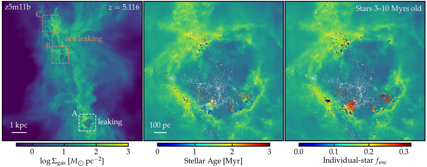
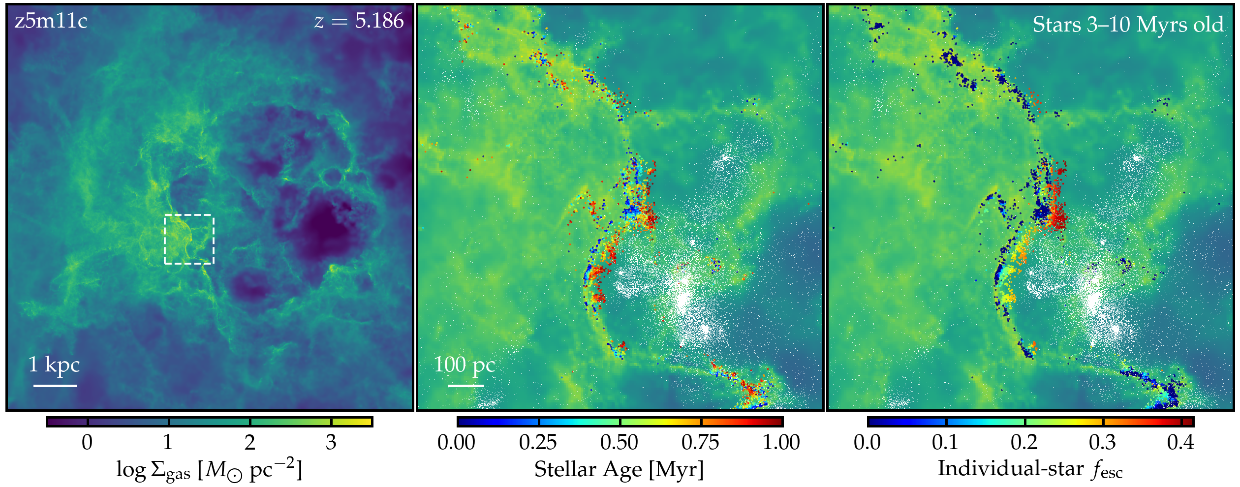
Figure 7: Examples of galaxies with strong ionizing photon leakage. Top row: The central galaxy in simulation z5m11b at $z=5.116$. The galaxy is at the early stage of a starburst. At this epoch, it has a halo (stellar) mass of $M_{\rm vir}=3.7\times 10^{10}\,M_{\sun}$ ($M_{\ast}=1.5\times 10^{8}\,M_{\sun}$) and instantaneous $f_{\rm esc}\sim 0.2$. Left: Gas surface density of a $10\,{\rm kpc}\times 10\,{\rm kpc}$ projection. Most stars in the past 10 Myr are formed in region A (marked by the white dashed square), where the majority of the escaped ionizing photons come from. Regions B and C have formed an order of magnitude fewer stars than region A, but almost no ionizing photons escape from both regions. Middle: Zoom-in image on region A (1.2 kpc on each side). The white points show stars 3–10 Myr old, while the color points show stars younger than 3 Myr, color-coded by their ages. Right: The same image as in the middle panel, except the young stars are color-coded by their single-star escape fractions. Region A contains a kpc-scale superbubble presumably created by stars 3–10 Myr old. A dense shell around the bubble is forming new stars while accelerated by feedback, leaving an age gradient at the bubble edge. Stars 2–3 Myr old are already in the low-density bubble. The large number of young stars in region A can fully ionize the low-column-density sightlines around the bubble, allowing a large fraction of ionizing photons to escape. In contrast, regions B and C do not contain a feedback-driven superbubble nor a large number of young stars to fully ionize the surrounding gas. Bottom row: The central galaxy of simulation z5m11c at $z=5.186$. The galaxy is in the middle of a starburst. It has a halo (stellar) mass of $M_{\rm vir}=7.4\times 10^{10}\,M_{\sun}$ ($M_{\ast}=7.8\times 10^{8}\,M_{\sun}$) and
instantaneous $f_{\rm esc}\sim 0.26$. The left panel shows the gas surface density of a $10\,{\rm kpc}\times 10\,{\rm kpc}$ projection. The white dashed square marks an active star-forming region where most of the escaped ionizing photons come from. The middle and right panels show the zoom-in image on this region. The white points show stars 3–10 Myr old and the color points show stars younger than 1 Myr, color-coded by stellar age (middle) and single-star escape fraction (right). This region contains a dense shell around a superbubble of several kpc in size. The shell is forming stars while accelerated presumably by feedback from stars 3–10 Myr nearby, so even stars 0.5–1 Myr old are already inside the shell, leaking 30–40% of their ionizing photons. We find such configuration (i.e. superbubble surrounded by a dense, accelerated shell) very common in strong ionizing-photon-leaking galaxies in our simulations, regardless of stellar mass and resolution.

4.1 Geometry of ionizing-photon-leaking regions

In this section, we present some example galaxies with strong ionizing photon leakage from our simulations to establish an intuitive picture for the escaping of ionizing photons. This is also useful for understanding the LyC-leaking galaxies discovered at intermediate and low redshifts (see Section 1 and references therein).

The top row of Fig. 7 shows the central galaxy of simulation z5m11b at $z=5.116$. The halo mass and stellar mass at this epoch are $M_{\rm vir}=3.7\times 10^{10}\,M_{\sun}$ and $M_{\ast}=1.5\times 10^{8}\,M_{\sun}$, respectively. It is at the early stage of starburst that begins 25 Myr ago. The galaxy has an instantaneous $f_{\rm esc}\sim 0.2$ and rapidly rising SFR at this time. The left panel presents the gas surface density of a 10 kpc$\times$10 kpc region centered at the halo center. A large gas reservoir has built up in the ISM that triggered the starburst ($M_{\rm gas}\sim 7.5\times 10^{8}\,M_{\sun}$ in the inner 5 kpc). Almost all star formation in the past 10 Myr happens in the three regions marked by the dashed squares (1.2 kpc on each side). Most stars were formed in region A (white). It is also where nearly all the escaped ionizing photons come from. Regions B and C (red) formed an order of magnitude fewer stars, and few ionizing photons from these stars can escape.

Region A contains a kpc-scale superbubble surrounded by an incomplete dense shell. In the top-middle panel of Fig. 7, we zoom into the 1.2 kpc$\times$1.2 kpc region marked by box A. The white points show stars formed 3–10 Myr ago, while the color points show stars younger than 3 Myr, color-coded by their ages. The top-right panel shows the same image, except that the young stars are color-coded by the escape fraction of individual stars. The superbubble is presumably created by clustered SNe from stars 3–10 Myr old. These stars are sitting in the low-density bubble at this time. In the meanwhile, new stars form in the compressed, dense shell as the bubble expands in the ISM. More importantly, the shell can be accelerated while forming stars. This is the reason why there is an age gradient in stars younger than 3 Myr at the bottom half of the shell (see also Yu et al., 2020). As a consequence, stars that are only 2–3 Myr old already locate inside the low-density bubble. Moreover, the bubble is not completely covered by dense gas, with a large fraction of the sightlines cleared by feedback along which the gas column density is low (e.g. the direction pointing out of the image). The bubble has a large number of young stars. We will show in Section 4.2 that the low-column-density sightlines can be fully ionized by these young stars, allowing ionizing photons to escape effectively through these optically-thin channels. Stars 3–10 Myr old in the bubble, and stars 2–3 Myr old at the inner side of the bubble (which have $f_{\rm esc}\sim 0.3$), contribute the majority of the escaped ionizing photons.

To summarize, region A is leaking ionizing photons along the optically-thin sightlines around the superbubble. The escaped photons come from stars 3–10 Myr old in the bubble and younger stars at the inner edge of the shell. The low-column-density channels are pre-cleared by feedback and then fully ionized by the large amount of young stars collectively in the bubble (cf. Fig. 8 and Section 4.2). In contrast, regions B and C do not contain a superbubble. We find that most of the young stars in these regions are still buried in their birth clouds. Even stars 3–10 Myr old are surrounded by optically-thick neutral gas in the ISM. This suggests that feedback in regions B and C has not been sufficiently strong to clear some channels that can be fully ionized to allow ionizing photons to escape.

The bottom row of Fig. 7 shows another example, the central galaxy in simulation z5m11c at $z=5.186$, when the galaxy is at the peak of a starburst. The halo (stellar) mass is $M_{\rm vir}=7.4\times 10^{10}\,M_{\sun}$ ($M_{\ast}=8\times 10^{8}\,M_{\sun}$) and instantaneous $f_{\rm esc}\sim 0.26$ at this time. The left panel shows the gas surface density in a 10 kpc$\times$10 kpc region around the halo center. The middle panel zooms into the $(1.2\,{\rm kpc})^{2}$ region marked by the white dashed box in the left. This region is at the edge of a superbubble of a few kpc in size and contains a dense shell compressed by the bubble. This is the most active star-forming region in the past 10 Myr, where the majority of the escaped ionizing photons come from. The white points show stars 3–10 Myr old, which locate inside the low-density bubble. The color points show stars younger than 1 Myr (rather than 3 Myr in the top row), color-coded by their age in the middle panel and by $f_{\rm esc}$ in the right panel. The shell is star-forming while accelerated presumably by the stars 3–10 Myr nearby, leading to the age gradient at the edge of the bubble. The low-column-density sightlines can be fully ionized by the young stars in this region, allowing ionizing photons to escape from these optically-thin paths. Even stars only 0.5–1 Myr old are inside the inner edge of the shell (in the low-density bubble), making 30–40% of their ionizing photons escape.

The two examples shown above share some similar features in regions that leak ionizing photons effectively. It must be an actively star-forming region that contains or is part of a kpc-scale superbubble. The bubble is surrounded by a compressed, dense shell where new stars form. The shell is usually accelerated, leaving an age gradient in the newly formed stars at the edge of the bubble. The bubble should not be fully confined, with low-column-density channels pre-cleared by feedback and fully ionized by the young stars in this region, from which ionizing photons can escape efficiently. Most of the escaped ionizing photons come from stars younger than 3 Myr in the inner edge of the shell and stars 3–10 Myr old inside the low-density bubble. We find such configuration very common in strong ionizing photon leakers (galaxies that have high $f_{\rm esc}$ and SFR at the same time) in our simulations, for galaxies of all masses and run at any mass resolution.

4.2 The important role of feedback

In the previous section, we use some examples to illustrate the typical geometry of strong ionizing-photon-leaking regions in galaxies with both high $f_{\rm esc}$ and SFR. In this section, we investigate the key physics that governs the escape of ionizing photons.

For a given star particle in our simulation, we can use the octree to calculate the hydrogen column density from the star particle to the virial radius of the halo along a given sightline, in which we use the ionization states determined by the MCRT code to compute the column density of neutral hydrogen. In Fig. 8, we compare the column density distribution for selected stars younger than 10 Myr in galaxies around $\log M_{\ast}\sim 8$ ($\pm 0.25$ dex; only simulations run at $900\,M_{\sun}$ are included), where the sample average $\langle f_{\rm esc}\rangle$ peaks at 0.2 (see Fig. 5). The black and red lines show stars with individual-star escape fraction $f_{\rm esc}<0.05$ and $f_{\rm esc}>0.2$, respectively. From every star particle, we compute the column density out to the virial radius along 100 random directions. Each stars is weighted equally when calculating the distribution function.

The solid lines show the distribution function of total (neutral and ionized) hydrogen column density ($N_{\rm H}=N_{\rm H\,I}+N_{\rm H\,II}$), while the dotted lines show that only for neutral hydrogen ($N_{\rm H\,I}$), with ionization states taken from our default MCRT calculations. As a proof of concept, we also redo the MCRT calculations without photoionization from stars (but including the uniform ionizing background and collisional ionization) and show the resulting distribution of $N_{\rm H\,I}$ in Fig. 8 with the thin dashed lines. Our results highlight two physical processes that are crucial to the escape of ionizing photons. First of all, comparing the black and red solid lines, we find that stars leaking ionizing photons effectively (e.g. $f_{\rm esc}>0.2$; red) tend to locate in regions with lower $N_{\rm H}$ around compared to stars that have much lower $f_{\rm esc}$ (black). These regions are presumably cleared by stellar feedback (e.g. SN bubbles; see Fig. 7 and Section 4.1). Second, we find a large fraction of optically-thin ($N_{\rm H\,I}\lesssim 2\times 10^{17}\,{\rm cm}^{-2}$) sightlines surrounding stars with high $f_{\rm esc}$, through which ionizing photons can escape freely. More importantly, comparing the red dashed and dotted lines, we argue that these optically-thin channels around young stars must be self-ionized by these stars. This is more likely to happen in regions where a large number of stars have formed in the past 10 Myr. In contrast, stars that have much lower $f_{\rm esc}$ tend to be fully embedded in optically-thick ($N_{\rm H\,I}\gg 2\times 10^{17}\,{\rm cm}^{-2}$) sightlines. These stars are not sufficient to highly ionize the surrounding gas, making it difficult for their ionizing photons to escape.

Although we only show the column density distribution for all stars younger than 10 Myr in galaxies around $\log M_{\ast}\sim 8$ in Fig. 8, we have confirmed that all our conclusions still hold if we compare stars in a narrow age bin or in galaxies at a different mass.

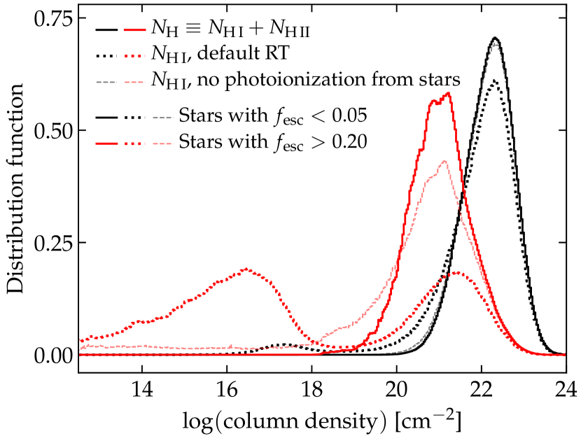
Figure 8: The distribution of gas column densities from stars $\lesssim 10$ Myr old in galaxies around $\log M_{\ast}\sim 8$ out to the halo virial radius. We include 100 random sightlines for each star particle. All stars are weighted equally. Only simulations at $m_{b}\sim 900\,M_{\sun}$ mass resolution are used in this analysis. The black and red colors represent stars with $f_{\rm esc}<0.05$ and $f_{\rm esc}>0.2$, respectively. The solid lines show the distribution of $N_{\rm H}$ (neutral and ionized). The high-$f_{\rm esc}$ stars tend to locate in regions surrounded by lower-$N_{\rm H}$ sightlines, likely cleared by feedback, than the low-$f_{\rm esc}$ stars. The dotted lines present the distribution of $N_{\rm H\,I}$, where we use the ionization states determined from our default MCRT calculations. As a proof of concept, the thin dashed lines show the distribution of $N_{\rm H\,I}$ without photoionization from stars. The high-$f_{\rm esc}$ stars are surrounded by a large fraction of optically-thin sightlines that must be ionized collectively by the young stars in the galaxy. However, the low-$f_{\rm esc}$ stars are almost fully covered by optically-thick sightlines.

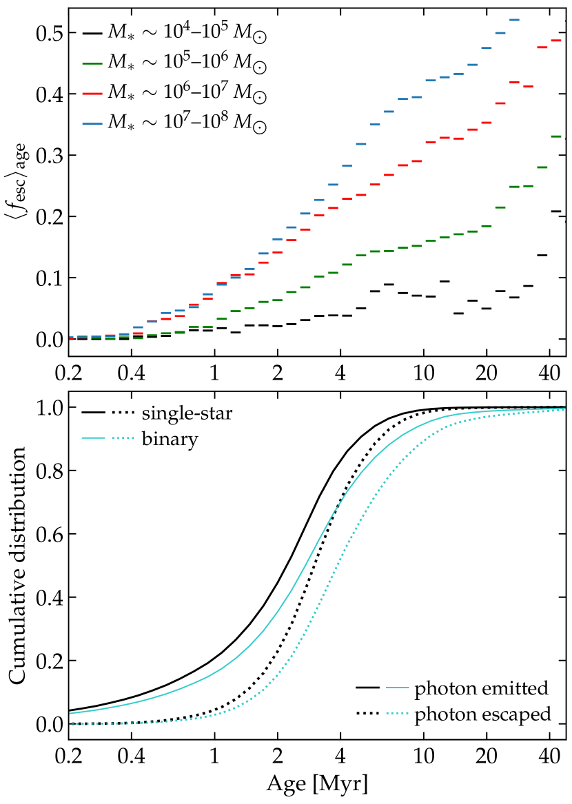
Figure 9: Top: The average escape fraction over individual stars in galaxies in four stellar mass bins for every $1/15$ dex in logarithmic age. Only simula- tions at $900\,M_{\sun}$ and better resolution are included. $\langle f_{\rm esc}\rangle_{\rm age}$ increases with stellar age for galaxies of all masses. $\langle f_{\rm esc}\rangle_{\rm age}$ increases with stellar mass at all ages, in line with the increase of sample average $\langle f_{\rm esc}\rangle$ with stellar mass in this mass range. Bottom: The cumulative distribution of ionizing photons emitted (solid) and escaped (dashed) as a function of stellar age. In single-star case (black), 50% of the escaped ionizing photons come from stars 1– 3 Myr old, while the rest 50% from stars 3–10 Myr old. The binary models extend the distribution to slightly later times.

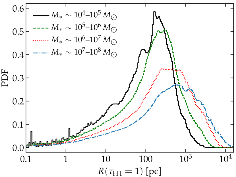
Figure 10: The distribution of radius from stars younger than 10 Myr out to which the optical depth of neutral hydrogen $\tau_{\rm H\,I}=1$ at the Lyman limit (a proxy to the distance an ionizing photon may travel) for galaxies in the four stellar mass bins. We include 100 random sightlines for each star particle and all stars are weighted equally. Only simulations at $900\,M_{\sun}$ resolution or better are included. In low-mass galaxies, about 60% of the sightlines from young stars become optically thick within 100 pc. The fraction of sightlines with $R(\tau_{\rm H\,I}=1)\gtrsim 100\,{\rm pc}$ and the median $R(\tau_{\rm H\,I}=1)$ increase with stellar mass, meaning a larger fraction of the ionizing photons can travel to longer distances in relatively high-mass galaxies. This indicates that feedback cannot clear the surroundings of young stars in low-mass galaxies.

4.3 Escape fraction by stellar age

We define the average of escape fraction over individual stars in a narrow age bin, $\langle f_{\rm esc}\rangle_{\rm age}$, for a selected population of galaxies from our simulations. In the top panel of Fig. 9, we present $\langle f_{\rm esc}\rangle_{\rm age}$ as a function of stellar age for galaxies in four stellar mass bins, where we calculate $\langle f_{\rm esc}\rangle_{\rm age}$ for every $\frac{1}{15}$ dex in logarithmic age. Note that we only use simulations at $900\,M_{\sun}$ or better resolution and single-star models for post-processing calculations.

We find $\langle f_{\rm esc}\rangle_{\rm age}$ increases with age for galaxies of all masses. A large fraction of the young stars are still embedded in their birth clouds, so they tend to have low $f_{\rm esc}$ on average. As feedback from these stars starts to destroy the birth clouds, blow out superbubbles in the ISM, and clear low-column-density sightlines, their ionizing photons can escape more easily, thereby increasing $\langle f_{\rm esc}\rangle_{\rm age}$ at later times. At a given age, $\langle f_{\rm esc}\rangle_{\rm age}$ tends to increase with stellar mass, in line with the trend between the sample average $\langle f_{\rm esc}\rangle$ and $M_{\ast}$ in Fig. 5. In more massive galaxies, stars 10 Myr old have an average $\langle f_{\rm esc}\rangle_{\rm age}\sim 0.4$; even stars 1–3 Myr old on average leak 10–20% of their ionizing photons, most of which are likely from stars formed in an accelerated shell at the edge of a superbubble (e.g. Fig. 7). In galaxies under $M_{\ast}\sim 10^{5}\,M_{\sun}$, however, almost no ionizing photon from stars younger than 3 Myr are able to escape; stars 10 Myr old only have $\langle f_{\rm esc}\rangle_{\rm age}$ lower than 0.1. After 20 Myr, $\langle f_{\rm esc}\rangle_{\rm age}$ increases more significantly with age, indicating that this is the time-scale on which feedback eventually clears some sightlines in such low-mass galaxies, but stars older than 20 Myr no longer have a high ionizing photon production efficiency.

For completeness, we show the cumulative distribution of ionizing photons emitted (solid) and escaped (dashed) as a function of stellar age in the bottom panel of Fig. 9. The distribution functions are calculated using all galaxies in our simulations at $900\,M_{\sun}$ resolution or better. We find nearly identical distributions for galaxies in a narrow mass bin or at $7000\,M_{\sun}$ resolution. When using single-star models (black), we find nearly 80% of the ionizing photons are emitted from stars younger than 3 Myr and the rest 20% from stars 3–10 Myr old, as the ionizing photon emissivity decreases dramatically after 3 Myr following the death of the most massive stars. As $\langle f_{\rm esc}\rangle_{\rm age}$ is low in the first Myr and increases with age, we find that nearly 50% of the escaped ionizing photons are from stars 1–3 Myr old and the other 50% from stars 3–10 Myr old. Alternatively, 90% of the escaped photons are from stars 1–5 Myr old.

In Section 3.2.3, we mention that binary models produce more ionizing photons after 3 Myr than single-star models owing to mass transfer and stellar mergers. These extra photons tend to escape efficiently given the relatively high $\langle f_{\rm esc}\rangle_{\rm age}$ after 3 Myr. When using binary models (cyan), we find 55% (35%) of the emitted (escaped) ionizing photons come from stars younger than 3 Myr, 40% (55%) from stars 3–10 Myr old, and the rest 5% (10%) from stars over 10 Myr old. We find binary stars only increase the number of ionizing photons escaped by 60–80%, much lower than that reported in previous works (cf. a factor of 3 or more; e.g. Ma et al., 2016; Rosdahl et al., 2018). This is likely due to the fact that a large fraction of the escaped ionizing photons are from stars younger than 3 Myr (when binary evolution is subdominant) in our simulations, thus reducing the relative effects of the extra photons from binaries after 3 Myr.

4.4 Why does $\langle f_{\rm esc}\rangle$ decrease at the low-mass end?

In Section 3.2.1 and Fig. 5, we show that the sample average $\langle f_{\rm esc}\rangle$ decreases with decreasing stellar mass below $M_{\ast}\sim 10^{8}\,M_{\sun}$. There is a similar trend with halo mass at $M_{\rm vir}\lesssim 10^{11}\,M_{\sun}$ if dust attenuation is ignored (e.g. the left column in Fig. 6). We study why $\langle f_{\rm esc}\rangle$ decreases at the low-mass in this section.

From each star particle younger than 10 Myr, we calculate the radius out to which the optically depth of H i $\tau_{\rm H\,I}=1$ at the Lyman limit from the particle along 100 random sightlines, using a similar method to what described in Section 4.2. This radius is an approximate measure to the distance an ionizing photon may travel before absorbed by neutral hydrogen. In Fig. 10, we show the distribution of this radius for galaxies in four stellar mass bins from $M_{\ast}\sim 10^{4}$–$10^{8}\,M_{\sun}$. Only simulations at $900\,M_{\sun}$ resolution or better are used. We weight all stars equally in the distribution functions. If a sightline has $\tau_{\rm H\,I}<1$ out to the virial radius, we set this radius to infinity
(not shown in Fig. 10, the fraction of such optically-thin sightlines increases with $M_{\ast}$). In low-mass galaxies ($M_{\ast}\lesssim 10^{5}\,M_{\sun}$), 60% of the sightlines from stars younger than 10 Myr turn optically thick in 100 pc. The fraction of sightlines with $R(\tau_{\rm H\,I}=1)\gtrsim 100\,{\rm pc}$, as well as the median $R(\tau_{\rm H\,I}=1)$, increases with stellar mass. The results in Fig. 10 suggest that most ionizing photons in low-mass galaxies are absorbed in a short range, while a larger fraction of the ionizing photons can reach larger distances (from a few 100 pc to 10 kpc) in relatively high-mass galaxies.

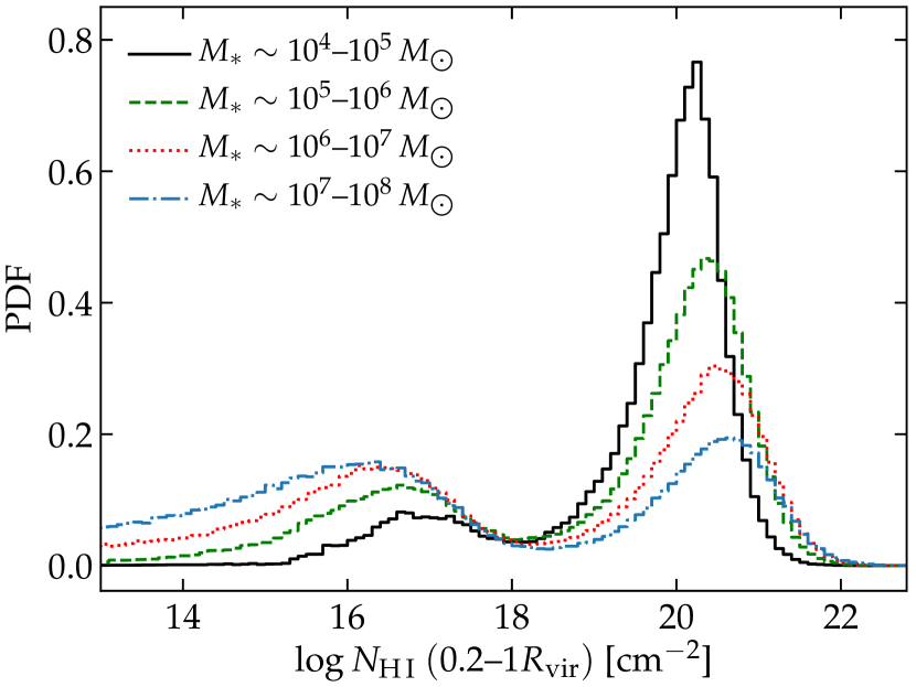
Figure 11: The distribution of $N_{\rm H\,I}$ integrated radially from 0.2–$1R_{\rm vir}$ in the halo of galaxies in four stellar mass bins. We include 1000 radial directions for each galaxy. All galaxies are equally weighted. The fraction of optically-thin sightlines increases with stellar mass. The low-mass galaxies are nearly fully surrounded by optically-thick gas in the halo.

In Fig. 11, we show the distribution of $N_{\rm H\,I}$ integrated radially from 0.2–$1R_{\rm vir}$ for galaxies in the same stellar mass bins, where we calculate $N_{\rm H\,I}$ along 1000 directions for each galaxy. We weight all galaxies equally. The distribution of $N_{\rm H\,I}$ from the outer ISM to the halo is bimodal, similar to the red dotted line in Fig. 8. The fraction of optically-thin sightlines ($N_{\rm H\,I}\lesssim 2\times 10^{17}\,{\rm cm}^{-2}$) decreases significantly with decreasing stellar mass. This suggests a high covering fraction of optically-thick neutral gas ($N_{\rm H\,I}\gtrsim 2\times 10^{17}\,{\rm cm}^{-2}$) in the halo around low-mass galaxies. We reiterate that the optically-thin paths are photoionized by the young stars collectively in the galaxy (cf. Fig. 8 and Section 4.2), presumably through some low-column-density paths channels pre-cleared by feedback.

In Ma et al. (2018), we show the stellar mass and average SFR scale with halo mass as $\propto M_{\rm vir}^{1.5}$, which means star formation is less efficient in low-mass galaxies than in their high-mass counterparts. Moreover, the mass-weighted gas temperature in the halo (roughly independent of radius in 0.2–$1R_{\rm vir}$) decreases from $10^{5}$ K for galaxies in $M_{\ast}\sim 10^{7}$–$10^{8}\,M_{\sun}$ to $10^{4}$ K for those in $M_{\ast}\sim 10^{4}$–$10^{5}\,M_{\sun}$, making collisional ionization less effective in the halo of low-mass galaxies. Combined the results from Figs. 9–11, we suggest that the low $\langle f_{\rm esc}\rangle$ in low-mass galaxies owes to a combination of reasons as follows. First, feedback is not strong enough to blow out kpc-scale superbubbles around stars $\lesssim 10$ Myr old and trigger star formation in the dense shell surrounding the bubble simultaneously. This can be seen from the fact that only a small fraction of the ionizing photons from young stars can travel more than 100 pc before absorbed in low-mass galaxies (Fig. 10). Second, the young stars cannot fully ionize a large number of channels throughout the halo (Fig. 11), so stars of all ages tend to have low escape fractions on average in the low-mass galaxies (the top panel in Fig. 9). Both arguments above are likely resulted from the low star formation efficiencies in these galaxies, namely low-mass galaxies do not form sufficient stars coherently to clear some low-column-density paths and to fully ionize these sightlines. Finally, the low gas temperatures in the halo make the neutral gas covering fraction higher around low-mass galaxies, at least partly responsible to the low $\langle f_{\rm esc}\rangle_{\rm age}$ in Fig. 9.

5 Discussion

5.1 The impact of sub-grid recipes

In Section 1, we mentioned that the prediction of $f_{\rm esc}$ from hydrodynamic simulations of galaxy formation might be sensitive to the ‘sub-grid’ models implemented in these simulations. In particular, Ma et al. (2015) found $\langle f_{\rm esc}\rangle\lesssim 0.05$ using a sample of three simulations spanning $M_{\rm vir}\sim 10^{9}$–$10^{11}\,M_{\sun}$ at $z\geq 5$ run with the FIRE-1 version of gizmo (see Hopkins et al., 2014, for details), whereas in this paper, we find $\langle f_{\rm esc}\rangle\sim 0.2$ in $M_{\rm vir}\sim 10^{9.5}$–$10^{11}\,M_{\sun}$ in FIRE-2 simulations, both using single-star stellar population models.

To test possible subtle effects of different sub-grid treatments, we re-run simulation z5m11b (with halo mass $M_{\rm vir}\sim 4\times 10^{10}\,M_{\sun}$ at $z=5$) from the initial condition to $z=5$ for more than 20 times with almost all possible combinations of choices for hydrodynamic method, sub-grid models, etc., as listed below.

• Hydrodynamic solver: P-SPH (Hopkins, 2013, used for FIRE-1) and MFM (Hopkins, 2015, FIRE-2).

• Density threshold for star formation in $n_{\rm th}=50$–$1000\,{\rm cm}^{-3}$. The default value for FIRE-1 (FIRE-2) is 50 (1000) cm^-3. We do not experiment with higher $n_{\rm th}$ given our resolution.

• The non-conservative FIRE-1 and the more accurate, conservative FIRE-2 SN coupling algorithms (see Hopkins et al., 2018a, for detailed descriptions and comparisons).

• The default self-gravitating criteria for star formation (used for both FIRE-1 and FIRE-2) and the stricter version from Grudić et al. (2018) (see also Ma et al. 2020).

• The star formation efficiency per local free-fall time $\epsilon\sim 0.1$–1 (default is 1 in both FIRE-1 and FIRE-2).

• The maximum search radius for gas particles for SN coupling in 0.2–10 kpc (default is 2 kpc in both FIRE-1 and FIRE-2).

• More subtle changes from FIRE-1 to FIRE-2 including the inclusion of an artificial pressure floor from Truelove et al. (1997) for the P-SPH method, cooling functions, and recombination rates.

All the tests we run produce statistically indistinguishable star formation histories for galaxy z5m10b. We also run post-processing calculations on all these simulations using our MCRT code to calculate $f_{\rm esc}$. We compare the time average of $f_{\rm esc}$ over 48 snapshots in $z=5$–10 for this galaxy, $\langle f_{\rm esc}\rangle_{t}$. We find that runs using the P-SPH method generally produce $\langle f_{\rm esc}\rangle_{t}\sim 0.1$, while those using the MFM method predict $\langle f_{\rm esc}\rangle_{t}\sim 0.2$. The star formation criteria, SN coupling algorithms, etc., make more subtle differences. Note that the P-SPH method smooths the density field using a quintic spline kernel over 64 nearest particles, thereby lowering the effective hydrodynamic resolution compared to the MFM method at the same particle mass. The difference in the hydrodynamic solver is in line with the difference in Fig. 5 between simulations at $7000\,M_{\sun}$ and those at $900\,M_{\sun}$ or better resolution, as some marginally optically-thin channels with $\tau_{\rm H\,I}\lesssim 1$ from which ionizing photons are able to escape would be under-resolved, or over-smoothed with optically-thick sightlines nearby and become $\tau_{\rm H\,I}\gtrsim 1$ at lower resolution.

However, we are not able to isolate the reason that causes the difference in $f_{\rm esc}$ between FIRE-1 and FIRE-2, presumably because of the complex, non-linear nature this problem.

In all the test runs, we identify the same configuration as those shown in Fig. 7 for vigorously star-forming regions where ionizing photons leak efficiently, namely a feedback-driven (sub-)kpc-scale superbubble surrounded by an accelerated, star-forming shell. New stars formed in the shell present a clear age gradient at the edge of the bubble, among which the relatively older ones, despite younger than 3 Myr, are already inside the low-density region. This happens in all sub-grid models of star formation and SN feedback we have tested (see also Yu et al., 2020). We caution that our simulations do not fully resolve the radiative shock at the front of the superbubble nor include a chemical network for dust and $\rm H_{2}$ molecule for more accurate star formation prescriptions, so we might not produce the correct amount of stars formed in the shell or the exact time-scale for star formation to happen there. However, we emphasize the fact that similar phenomenon has been observed as supergiant shells in the Large Magellanic Clouds (e.g. Pellegrini et al. 2012; Dawson et al. 2013; see also supershells and propagated star formation, e.g. Heiles 1979; McCray & Kafatos 1987).

5.2 Which galaxies provide the most ionizing photons?

In Section 3.2.1, we find $\langle f_{\rm esc}\rangle$ increases with halo mass in $M_{\rm vir}\sim 10^{8}$–$10^{9.5}\,M_{\sun}$, turns nearly constant in $M_{\rm vir}\sim 10^{9.5}$–$10^{11}\,M_{\sun}$, and decreases with halo mass above $M_{\rm vir}\sim 10^{11}\,M_{\sun}$. In the literature, the dependence of $\langle f_{\rm esc}\rangle$ on $M_{\rm vir}$ has been studied in state-of-the-art simulations with sophisticated chemical network and/or on-the-fly radiation-hydrodynamics. These simulations are fairly expensive so some of them are run in small cosmological volumes (box size less than $\sim 10\,{\rm cMpc}$) and/or stopped at relatively high redshifts ($z\gtrsim 8$) (see e.g. Wise et al. 2014; O’Shea et al. 2015; Paardekooper et al. 2015; Xu et al. 2016). These studies found that $\langle f_{\rm esc}\rangle$ decrease with halo mass, from $\langle f_{\rm esc}\rangle\sim 0.5$ at $M_{\rm vir}\lesssim 10^{7}\,M_{\sun}$ to $\langle f_{\rm esc}\rangle\lesssim 0.05$ at $M_{\rm vir}\gtrsim 10^{8}\,M_{\sun}$ (e.g. Wise et al., 2014; Xu et al., 2016). Intriguingly, Xu et al. (2016) found that $\langle f_{\rm esc}\rangle$ starts to increase at $M_{\rm vir}\gtrsim 10^{9}\,M_{\sun}$ to $\langle f_{\rm esc}\rangle\sim 0.1$–0.2 at $M_{\rm vir}\sim 10^{9.5}\,M_{\sun}$, in line with what we find in our simulations. Nonetheless, the simulation from Xu et al. (2016) only contains a small number of halos at $M_{\rm vir}\sim 10^{9.5}\,M_{\sun}$ while no halo at higher masses. Our results thus complement these previous studies by extending the $\langle f_{\rm esc}\rangle$–$M_{\rm vir}$ relation to the massive end.

In our simulations, the average SFR, and thereby the ionizing photon emissivity $\langle Q_{\rm ion}\rangle$, scale with halo mass as $\propto M_{\rm vir}^{1.5}$. A nearly constant $\langle f_{\rm esc}\rangle$ gives $\langle Q_{\rm esc}\rangle\propto M_{\rm vir}^{1.5}$ for the rates of escaped photons at intermediate halo mass from $M_{\rm vir}\sim 10^{9}$–$10^{11}\,M_{\sun}$, which is also confirmed directly in our post-processing calculations. The scaling becomes steeper (shallower) as $\langle Q_{\rm esc}\rangle\propto M_{\rm vir}^{2.5}$ ($\propto M_{\rm vir}^{1.0}$) at the low- (high-)mass end as $\langle f_{\rm esc}\rangle$ decreases. At a given halo mass, both the SFR (and hence $\langle Q_{\rm ion}\rangle$) and $\langle f_{\rm esc}\rangle$ increase with redshift (see fig. 7 in Ma et al. 2018 and Fig. 6), so $\langle Q_{\rm esc}\rangle$ also increases with redshift. The best-fit normalization of the broken power-law function to our data is $\langle Q_{\rm esc}\rangle\sim 1$–$4\times 10^{53}\,{\rm s}^{-1}$ from $z=6$–10 at $M_{\rm vir}=10^{11}\,M_{\sun}$, where we use single-star stellar population models. By convolving the broken power-law function of $\langle Q_{\rm esc}\rangle$–$M_{\rm vir}$ relation with the halo mass functions (HMFs; Murray et al., 2013) at $z\geq 5$, we obtain the number density of ionizing photons escaped to the IGM as $\dot{n}_{\rm ion}\sim 10^{51.2}$–$10^{50.6}\,{\rm s}^{-1}\,{\rm Mpc}^{-3}$, decreasing with redshift from $z=6$ to 10. Binary stars will enhance $\dot{n}_{\rm ion}$ by about $\sim 60$–80% (Section 3.2.3). Our estimate of $\dot{n}_{\rm ion}$ is in broad agreement with what derived from the most recent constraints on the reionization history (e.g. Mason et al., 2019b). Here we present the quantitative details on $\langle Q_{\rm esc}\rangle$ and $\dot{n}_{\rm ion}$ only for completeness. Given the non-convergence in our simulations, we emphasize that these numbers likely suffer a factor of 2 uncertainties. They should be used with caution.

Now we consider the distribution of $\dot{n}_{\rm ion}$ per logarithmic halo mass, ${\rm d}\dot{n}_{\rm ion}/{\rm d}\log M_{\rm vir}$. The HMF can be well described by a power-law function at the low-mass end and an exponential function at the high-mass end, ${\rm d}n/{\rm d}\log M_{\rm vir}\sim M_{\rm vir}^{1-\alpha}\exp(-M_{\rm vir}/M_{\rm vir}^{\ast})$, where $M_{\rm vir}^{\ast}$ is some characteristic mass (Schechter, 1976). As ${\rm d}\dot{n}_{\rm ion}/{\rm d}\log M_{\rm vir}=\langle Q_{\rm esc}\rangle\,{\rm d}n/{\rm d}\log M_{\rm vir}$, for the canonical $\alpha=2$ slope, ${\rm d}\dot{n}_{\rm ion}/{\rm d}\log M_{\rm vir}$ increases with $M_{\rm vir}$ at the low-mass end and decreases dramatically above $M_{\rm vir}^{\ast}$. We find at $z\sim 6$, ${\rm d}\dot{n}_{\rm ion}/{\rm d}\log M_{\rm vir}$ peaks at approximate $M_{\rm vir}\sim 10^{10.5}\,M_{\sun}$ ($M_{\ast}\sim 10^{8}\,M_{\sun}$), which means that intermediate-mass galaxies dominate the cosmic ionizing photon budget at $z\sim 6$ (see also Naidu et al., 2020). However, the HMF starts to decline at a much smaller mass at $z\sim 10$, so we find ${\rm d}\dot{n}_{\rm ion}/{\rm d}\log M_{\rm vir}$ peaks at $M_{\rm vir}\sim 10^{9}\,M_{\sun}$ ($M_{\ast}\lesssim 10^{6}\,M_{\sun}$). Our results suggest that low-mass galaxies dominate the ionizing photon budget at early times, while more massive galaxies take over near the end of reionization (e.g. Finkelstein et al., 2012, 2019; Robertson et al., 2013; Robertson et al., 2015; Faucher-Giguère, 2020; Naidu et al., 2020; Yung et al., 2020).

6 Conclusions

In this paper, we use a sample of 34 high-resolution cosmological zoom-in simulations of $z\geq 5$ galaxies run with the FIRE-2 version of the source code gizmo and explicit models for the multi-phase ISM, star formation, and stellar feedback in Hopkins et al. (2018b). Our sample consists of simulations run at baryonic mass resolution $m_{b}\sim 7000\,M_{\sun}$, $900\,M_{\sun}$, and $100\,M_{\sun}$. We post-process over 8500 relatively well-resolved galaxy snapshots from all zoom-in regions with a Monte Carlo radiative transfer code for ionizing radiation to calculate $f_{\rm esc}$ and the gas ionization states. Our default calculations assume a constant dust-to-metal ratio of 0.4 in gas below $10^{6}$ K (no dust at higher temperatures) and a SMC-like extinction curve from Weingartner & Draine (2001). We consider both the single-star and binary models from the BPASS stellar population synthesis models to calculate the ionizing photon emissivity for every star particle in our simulations (v2.2.1; Eldridge et al., 2017).

We study the sample average $\langle f_{\rm esc}\rangle$ (i.e. the average of instantaneous $f_{\rm esc}$ over all galaxies at all redshifts for a given halo/stellar mass bin) and its dependence on halo or stellar mass, redshift, dust, and stellar population models. We also explore the key physics that governs the escape of ionizing photons in our simulations.

Our main findings include the following.

(i) Both the instantaneous $f_{\rm esc}$ and SFR exhibit strong variability on short time-scales (Section 3.1, Fig. 3). There is usually a time delay between the rising of $f_{\rm esc}$ and the rising of SFR at the beginning of a starburst, because it takes some time for feedback to clear the sightlines for ionizing photons to escape. A galaxy may have a high $f_{\rm esc}$ but low SFR at some epochs, meaning that it is not leaking a large number of ionizing photons. The instantaneous $f_{\rm esc}$–$M_{\rm vir}$ relation shows enormous scatter, with $f_{\rm esc}$ ranging from $\lesssim 10^{-4}$ to 1 at fixed $M_{\rm vir}$ (Fig. 4).

(ii) Our results on the sample average $\langle f_{\rm esc}\rangle$ do not fully converge with resolution. Simulations run at $7000\,M_{\sun}$ resolution tend to produce systematically lower $\langle f_{\rm esc}\rangle$ than those run at $900\,M_{\sun}$ or better resolution. Simulations with 900 and $100\,M_{\sun}$ resolution produce consistent results on $\langle f_{\rm esc}\rangle$. Nonetheless, the qualitative trends in the $\langle f_{\rm esc}\rangle$–$M_{\rm vir}$ ($M_{\ast}$) relation are robust (Section 3.2.1, Fig. 5).

(iii) In our default dust model, $\langle f_{\rm esc}\rangle$ increases with halo mass in $M_{\rm vir}\sim 10^{8}$–$10^{9.5}\,M_{\sun}$, becomes roughly constant in $M_{\rm vir}\sim 10^{9.5}$–$10^{11}\,M_{\sun}$, and decreases at $M_{\rm vir}\gtrsim 10^{11}\,M_{\sun}$ (left, Fig. 5). $\langle f_{\rm esc}\rangle$ also increases with stellar mass in $M_{\ast}\sim 10^{4}$– $10^{8}\,M_{\sun}$ and decreases at $M_{\ast}\gtrsim 10^{8}\,M_{\sun}$ (right, Fig. 5). The declining $\langle f_{\rm esc}\rangle$ at the high-mass end is due to dust attenuation (Section 3.2.2; left column, Fig. 6).

(iv) For single-star models, $\langle f_{\rm esc}\rangle\sim 0.2$ around $M_{\ast}\sim 10^{8}\,M_{\sun}$ and $M_{\rm vir}\sim 10^{10.5}\,M_{\sun}$ (for simulations at $900\,M_{\sun}$ or better resolution, $\langle f_{\rm esc}\rangle\sim 0.1$ for those at $7000\,M_{\sun}$ resolution). The binary stars boost $\langle f_{\rm esc}\rangle$ by 25–35%, the ionizing photon emissivity by 20–30%, and therefore the number of photons escaped by 60–80% (Section 3.2.3; middle column, Fig. 6). The effect of binary stars is modest, as a considerable fraction of stars younger than 3 Myr leak ionizing photons efficiently (see below).

(v) Galaxies at $z\geq 8$ tend to have systematically higher $\langle f_{\rm esc}\rangle$ than those at $z<8$, suggesting a decreasing $f_{\rm esc}$ toward lower redshift (right column, Fig. 6).

(vi) We find a common geometry for vigorously star-forming regions that leak ionizing photons efficiently. They usually contain (or a part of) a feedback-driven, kpc-scale superbubble surrounded by a dense, star-forming shell. The shell is also accelerated, leaving an age gradient in the newly formed stars at the bubble edge. Stars formed slightly earlier in the shell, despite younger than 3 Myr, are already at the inner side of the shell. These young stars, along with stars 3–10 Myr old in the bubble, can fully ionize the low-column-density sightlines surrounding the bubble, allowing a large fraction of their ionizing photons to escape (Section 4.1, Fig. 7).

(vii) Young stars ($\lesssim 10$ Myr) with high $f_{\rm esc}$ (measured for individual stars) preferentially locate in regions with lower column densities out to the virial radius, compared to stars with low $f_{\rm esc}$. These regions are presumably cleared by stellar feedback. In addition, the low-column-density sightlines must also be ionized collectively by the young stars in these regions to become optically thin to ionizing photons. In contrast, stars with low $f_{\rm esc}$ are fully hidden in optically-thick sightlines (Section 4.2, Fig. 8).

(viii) The average of $f_{\rm esc}$ over stars in a given age, $\langle f_{\rm esc}\rangle_{\rm age}$, increases monotonically with stellar age in 0–40 Myr, likely because the impact of feedback in clearing the sightlines gets stronger with time. At fixed age, $\langle f_{\rm esc}\rangle_{\rm age}$ decreases in galaxies with decreasing stellar mass in $M_{\ast}\sim 10^{4}$–$10^{8}\,M_{\sun}$, in line with the $\langle f_{\rm esc}\rangle$–$M_{\ast}$ relation at the low-mass end (Section 4.3, Fig. 9).

(ix) In single-star models, about a half of the escaped ionizing photons come from stars 1–3 Myr old, while the rest from stars 3–10 Myr old. The contribution from stars $\gtrsim 10$ Myr old is negligible. In binary models, 35%, 45%, and 20% of the escaped photons are from stars 1–3, 3–10, and $\gtrsim 10$ Myr old (Section 4.3, Fig. 9).

(x) With decreasing stellar mass at $M_{\ast}\lesssim 10^{8}\,M_{\sun}$, an increasing fraction of the ionizing photons are absorbed in a shorter range (Fig. 10) and the covering fraction of optically-thick gas in the halo also increases (Fig. 11). This suggests that the low $\langle f_{\rm esc}\rangle$ at the low-mass end is due to a combination of inefficient star formation (and hence feedback) and low gas temperatures in the halo (Section 4.4).

(xi) We estimate the escaped ionizing photon density based on simple broken power-law fits to our simulation data, $\dot{n}_{\rm ion}\sim 10^{50.6}$–$10^{51.2}\,{\rm s}^{-1}\,{\rm Mpc}^{-3}$, increasing with decreasing redshift from $z=6$ to 10. This is sufficient for cosmic reionization according to most recent constraints. We find low-mass galaxies ($M_{\ast}\lesssim 10^{6}\,M_{\sun}$) dominate the cosmic ionizing photon budget at $z\sim 10$, but intermediate-mass galaxies ($M_{\ast}\sim 10^{8}\,M_{\sun}$) gradually take over toward the end of reionization at $z\sim 6$ (Section 5.2).

In future work, we will carry out radiative transfer calculations on the resonance Lyman-$\alpha$ line (e.g. Smith et al., 2019) and nebular lines like [O ii] and [O iii] (e.g. Arata et al., 2020) to understand the proposed observational signatures of $f_{\rm esc}$ (Section 1, and references therein). We will also revisit the question of $f_{\rm esc}$ as we keep improving our sub-grid recipes, resolution, and numerical methods.

Data Availability Statement

The data underlying this article will be shared on reasonable request to the corresponding author.

Appendix A The effect of resolution on $\langle f_{\rm esc}\rangle$

In Section 3.2, we show the sample-averaged $\langle f_{\rm esc}\rangle$ does not fully converge with resolution, with simulations at $m_{b}\sim 7000\,M_{\sun}$ resolution producing systematically lower $\langle f_{\rm esc}\rangle$ than those at $900\,M_{\sun}$ or better resolution (Fig. 5). We further show in Fig. 12 the column density distribution from stars younger than 10 Myr out to the halo virial radius in galaxies around $\log M_{\ast}\sim 8$. From each particle, we calculate the column densities along 100 random sightlines and the distribution functions are weighted by the ionizing photon emissivity. The solid and dashed lines show $N_{\rm H}$ and $N_{\rm H\,I}$, respectively. The colors represent simulations at $\lesssim 900\,M_{\sun}$ (blue) and $\sim 7000\,M_{\sun}$ (orange) resolution. At higher resolution, the distribution of $N_{\rm H}$ extends to lower column densities and hence a higher fraction of the sightlines become optically thin ($N_{\rm H\,I}\lesssim 2\times 10^{17}\,{\rm cm}^{-2}$) to ionizing photons than at lower resolution. We speculate that the primary reason for the lower $\langle f_{\rm esc}\rangle$ at lower resolution is that some of the low-column-density, optically-thin sightlines would be under-resolved, or over-smoothed and hence becomes optically thick at lower resolution, consistent with our findings in Section 5.1 that SPH method tends to produce systematically lower $f_{\rm esc}$ than MFM method given the lower effective hydrodynamic resolution with SPH method. We emphasize the importance of convergence study when studying $f_{\rm esc}$ in hydrodynamic simulations.

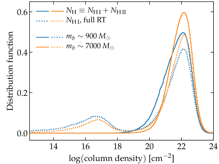
Figure 12: Column density distribution from stars $\lesssim 10$ Myr old out to the halo virial radius in galaxies around $\log M_{\ast}\sim 8$. The solid and dashed lines show $N_{\rm H}$ and $N_{\rm H\,I}$, respectively. The blue and orange lines show simulations
at $m_{b}\lesssim 900\,M_{\sun}$ and $\sim 7000\,M_{\sun}$ resolution, respectively. At higher resolution, the distribution of $N_{\rm H}$ extends to lower column densities and a larger
fraction of sightlines are optically thin, therefore resulting in systematically higher $\langle f_{\rm esc}\rangle$ at higher resolution.

References

- Anderson et al. (2017) Anderson L., Governato F., Karcher M., Quinn T., Wadsley J., 2017, MNRAS, 468, 4077
- Arata et al. (2020) Arata S., Yajima H., Nagamine K., Abe M., Khochfar S., 2020, preprint (arXiv:2001.01853)
- Atek et al. (2015) Atek H. et al., 2015, ApJ, 814, 69
- Atek et al. (2018) Atek H., Richard J., Kneib J.-P., Schaerer D., 2018, MNRAS, 479, 5184
- Becker et al. (2015) Becker G. D., Bolton J. S., Madau P., Pettini M., Ryan-Weber E. V., Venemans B. P., 2015, MNRAS, 447, 3402
- Boutsia et al. (2011) Boutsia K. et al., 2011, ApJ, 736, 41
- Bouwens et al. (2015a) Bouwens R. J. et al., 2015a, ApJ, 803, 34
- Bouwens et al. (2015b) Bouwens R. J., Illingworth G. D., Oesch P. A., Caruana J., Holwerda B., Smit R., Wilkins S., 2015b, ApJ, 811, 140
- Bouwens et al. (2016) Bouwens R. J. et al., 2016, ApJ, 830, 67
- Bouwens et al. (2017) Bouwens R. J., Oesch P. A., Illingworth G. D., Ellis R. S., Stefanon M., 2017, ApJ, 843, 129
- Bowler et al. (2015) Bowler R. A. A. et al., 2015, MNRAS, 452, 1817
- Bridge et al. (2010) Bridge C. R. et al., 2010, ApJ, 720, 465
- Bryan & Norman (1998) Bryan G. L., Norman M. L., 1998, ApJ, 495, 80
- Ceverino et al. (2017) Ceverino D., Glover S. C. O., Klessen R. S., 2017, MNRAS, 470, 2791
- Chisholm et al. (2018) Chisholm J. et al., 2018, A&A, 616, A30
- Conroy (2013) Conroy C., 2013, ARA&A, 51, 393
- Conroy & Kratter (2012) Conroy C., Kratter K. M., 2012, ApJ, 755, 123
- Cowie et al. (2009) Cowie L. L., Barger A. J., Trouille L., 2009, ApJ, 692, 1476
- Dawson et al. (2013) Dawson J. R., McClure-Griffiths N. M., Wong T., Dickey J. M., Hughes A., Fukui Y., Kawamura A., 2013, ApJ, 763, 56
- Dwek (1998) Dwek E., 1998, ApJ, 501, 643
- Eldridge & Stanway (2012) Eldridge J. J., Stanway E. R., 2012, MNRAS, 419, 479
- Eldridge et al. (2017) Eldridge J. J., Stanway E. R., Xiao L., McClelland L. A. S., Taylor G., Ng M., Greis S. M. L., Bray J. C., 2017, PASA, 34, e058
- Escala et al. (2018) Escala I. et al., 2018, MNRAS, 474, 2194
- Fan et al. (2006a) Fan X., Carilli C. L., Keating B., 2006a, ARA&A, 44, 415
- Fan et al. (2006b) Fan X. et al., 2006b, AJ, 132, 117
- Faucher-Giguère (2020) Faucher-Giguère C.-A., 2020, MNRAS, 493, 1614
- Faucher-Giguère et al. (2009) Faucher-Giguère C.-A., Lidz A., Zaldarriaga M., Hernquist L., 2009, ApJ, 703, 1416
- Ferland et al. (2013) Ferland G. J. et al., 2013, RMxAA, 49, 137
- Ferrara & Loeb (2013) Ferrara A., Loeb A., 2013, MNRAS, 431, 2826
- Finkelstein et al. (2012) Finkelstein S. L. et al., 2012, ApJ, 758, 93
- Finkelstein et al. (2015) Finkelstein S. L. et al., 2015, ApJ, 810, 71
- Finkelstein et al. (2019) Finkelstein S. L. et al., 2019, ApJ, 879, 36
- Fletcher et al. (2019) Fletcher T. J., Tang M., Robertson B. E., Nakajima K., Ellis R. S., Stark D. P., Inoue A., 2019, ApJ, 878, 87
- Fumagalli et al. (2011) Fumagalli M., Prochaska J. X., Kasen D., Dekel A., Ceverino D., Primack J. R., 2011, MNRAS, 418, 1796
- Gnedin (2016) Gnedin N. Y., 2016, ApJ, 825, L17
- Gnedin et al. (2008) Gnedin N. Y., Kravtsov A. V., Chen H.-W., 2008, ApJ, 672, 765
- Götberg et al. (2017) Götberg Y., de Mink S. E., Groh J. H., 2017, A&A, 608, A11
- Götberg et al. (2020) Götberg Y., de Mink S. E., McQuinn M., Zapartas E., Groh J. H., Norman C., 2020, A&A, 634, A134
- Grazian et al. (2016) Grazian A. et al., 2016, A&A, 585, A48
- Grazian et al. (2017) Grazian A. et al., 2017, A&A, 602, A18
- Grudić et al. (2018) Grudić M. Y., Hopkins P. F., Faucher-Giguère C.-A., Quataert E., Murray N., Kereš D., 2018, MNRAS, 475, 3511
- Haardt & Madau (2012) Haardt F., Madau P., 2012, ApJ, 746, 125
- Hahn & Abel (2011) Hahn O., Abel T., 2011, MNRAS, 415, 2101
- Heiles (1979) Heiles C., 1979, ApJ, 229, 533
- Hopkins (2013) Hopkins P. F., 2013, MNRAS, 428, 2840
- Hopkins (2015) Hopkins P. F., 2015, MNRAS, 450, 53
- Hopkins et al. (2013) Hopkins P. F., Narayanan D., Murray N., 2013, MNRAS, 432, 2647
- Hopkins et al. (2014) Hopkins P. F., Kereš D., Oñorbe J., Faucher-Giguère C.-A., Quataert E., Murray N., Bullock J. S., 2014, MNRAS, 445, 581
- Hopkins et al. (2018a) Hopkins P. F. et al., 2018a, MNRAS, 477, 1578
- Hopkins et al. (2018b) Hopkins P. F. et al., 2018b, MNRAS, 480, 800
- Hopkins et al. (2020) Hopkins P. F., Grudić M. Y., Wetzel A., Kereš D., Faucher-Giguère C.-A., Ma X., Murray N., Butcher N., 2020, MNRAS, 491, 3702
- Izotov et al. (2016a) Izotov Y. I., Schaerer D., Thuan T. X., Worseck G., Guseva N. G., Orlitová I., Verhamme A., 2016a, MNRAS, 461, 3683
- Izotov et al. (2016b) Izotov Y. I., Orlitová I., Schaerer D., Thuan T. X., Verhamme A., Guseva N. G., Worseck G., 2016b, Nature, 529, 178
- Izotov et al. (2018) Izotov Y. I., Schaerer D., Worseck G., Guseva N. G., Thuan T. X., Verhamme A., Orlitová I., Fricke K. J., 2018, MNRAS, 474, 4514
- Izotov et al. (2020) Izotov Y. I., Schaerer D., Worseck G., Verhamme A., Guseva N. G., Thuan T. X., Orlitová I., Fricke K. J., 2020, MNRAS, 491, 468
- Jaskot & Oey (2014) Jaskot A. E., Oey M. S., 2014, ApJ, 791, L19
- Jaskot et al. (2019) Jaskot A. E., Dowd T., Oey M. S., Scarlata C., McKinney J., 2019, ApJ, 885, 96
- Jefferies (1968) Jefferies J. T., 1968, Spectral line formation
- Ji et al. (2020) Ji Z. et al., 2020, ApJ, 888, 109
- Kakiichi & Gronke (2019) Kakiichi K., Gronke M., 2019, preprint (arXiv:1905.02480)
- Kakiichi et al. (2018) Kakiichi K. et al., 2018, MNRAS, 479, 43
- Katz et al. (1996) Katz N., Weinberg D. H., Hernquist L., 1996, ApJS, 105, 19
- Keenan et al. (2017) Keenan R. P., Oey M. S., Jaskot A. E., James B. L., 2017, ApJ, 848, 12
- Kim et al. (2013) Kim J.-h., Krumholz M. R., Wise J. H., Turk M. J., Goldbaum N. J., Abel T., 2013, ApJ, 775, 109
- Kim et al. (2019) Kim J.-G., Kim W.-T., Ostriker E. C., 2019, ApJ, 883, 102
- Kimm & Cen (2014) Kimm T., Cen R., 2014, ApJ, 788, 121
- Kimm et al. (2017) Kimm T., Katz H., Haehnelt M., Rosdahl J., Devriendt J., Slyz A., 2017, MNRAS, 466, 4826
- Knollmann & Knebe (2009) Knollmann S. R., Knebe A., 2009, ApJS, 182, 608
- Kroupa (2002) Kroupa P., 2002, Science, 295, 82
- Kuhlen & Faucher-Giguère (2012) Kuhlen M., Faucher-Giguère C.-A., 2012, MNRAS, 423, 862
- Leitet et al. (2011) Leitet E., Bergvall N., Piskunov N., Andersson B.-G., 2011, A&A, 532, A107
- Leitet et al. (2013) Leitet E., Bergvall N., Hayes M., Linné S., Zackrisson E., 2013, A&A, 553, A106
- Leitherer et al. (1995) Leitherer C., Ferguson H. C., Heckman T. M., Lowenthal J. D., 1995, ApJ, 454, L19
- Leitherer et al. (1999) Leitherer C. et al., 1999, ApJS, 123, 3
- Livermore et al. (2017) Livermore R. C., Finkelstein S. L., Lotz J. M., 2017, ApJ, 835, 113
- Loeb & Barkana (2001) Loeb A., Barkana R., 2001, ARA&A, 39, 19
- Ma et al. (2015) Ma X., Kasen D., Hopkins P. F., Faucher-Giguère C.-A., Quataert E., Kereš D., Murray N., 2015, MNRAS, 453, 960
- Ma et al. (2016) Ma X., Hopkins P. F., Kasen D., Quataert E., Faucher-Giguère C.-A., Kereš D., Murray N., Strom A., 2016, MNRAS, 459, 3614
- Ma et al. (2018) Ma X. et al., 2018, MNRAS, 478, 1694
- Ma et al. (2019) Ma X. et al., 2019, MNRAS, 487, 1844
- Ma et al. (2020) Ma X. et al., 2020, MNRAS, 493, 4315
- Madau & Haardt (2015) Madau P., Haardt F., 2015, ApJ, 813, L8
- Madau et al. (1999) Madau P., Haardt F., Rees M. J., 1999, ApJ, 514, 648
- Malkan & Malkan (2019) Malkan M. A., Malkan B. K., 2019, preprint (arXiv:1912.10970)
- Mannucci et al. (2006) Mannucci F., Della Valle M., Panagia N., 2006, MNRAS, 370, 773
- Mason et al. (2018) Mason C. A., Treu T., Dijkstra M., Mesinger A., Trenti M., Pentericci L., de Barros S., Vanzella E., 2018, ApJ, 856, 2
- Mason et al. (2019a) Mason C. A. et al., 2019a, MNRAS, 485, 3947
- Mason et al. (2019b) Mason C. A., Naidu R. P., Tacchella S., Leja J., 2019b, MNRAS, 489, 2669
- McCray & Kafatos (1987) McCray R., Kafatos M., 1987, ApJ, 317, 190
- Menacho et al. (2019) Menacho V. et al., 2019, MNRAS, 487, 3183
- Mesinger et al. (2015) Mesinger A., Aykutalp A., Vanzella E., Pentericci L., Ferrara A., Dijkstra M., 2015, MNRAS, 446, 566
- Micheva et al. (2018) Micheva G., Oey M. S., Keenan R. P., Jaskot A. E., James B. L., 2018, ApJ, 867, 2
- Murray et al. (2013) Murray S. G., Power C., Robotham A. S. G., 2013, Astronomy and Computing, 3, 23
- Naidu et al. (2020) Naidu R. P., Tacchella S., Mason C. A., Bose S., Oesch P. A., Conroy C., 2020, ApJ, 892, 109
- Nakajima & Ouchi (2014) Nakajima K., Ouchi M., 2014, MNRAS, 442, 900
- Nakajima et al. (2020) Nakajima K., Ellis R. S., Robertson B. E., Tang M., Stark D. P., 2020, ApJ, 889, 161
- Nestor et al. (2013) Nestor D. B., Shapley A. E., Kornei K. A., Steidel C. C., Siana B., 2013, ApJ, 765, 47
- Oñorbe et al. (2014) Oñorbe J., Garrison-Kimmel S., Maller A. H., Bullock J. S., Rocha M., Hahn O., 2014, MNRAS, 437, 1894
- O’Shea et al. (2015) O’Shea B. W., Wise J. H., Xu H., Norman M. L., 2015, ApJ, 807, L12
- Ocvirk et al. (2016) Ocvirk P. et al., 2016, MNRAS, 463, 1462
- Oesch et al. (2013) Oesch P. A. et al., 2013, ApJ, 773, 75
- Oesch et al. (2014) Oesch P. A. et al., 2014, ApJ, 786, 108
- Ono et al. (2018) Ono Y. et al., 2018, PASJ, 70, S10
- Paardekooper et al. (2011) Paardekooper J.-P., Pelupessy F. I., Altay G., Kruip C. J. H., 2011, A&A, 530, A87
- Paardekooper et al. (2015) Paardekooper J.-P., Khochfar S., Dalla Vecchia C., 2015, MNRAS, 451, 2544
- Pellegrini et al. (2012) Pellegrini E. W., Oey M. S., Winkler P. F., Points S. D., Smith R. C., Jaskot A. E., Zastrow J., 2012, ApJ, 755, 40
- Planck Collaboration et al. (2016a) Planck Collaboration et al., 2016a, A&A, 594, A13
- Planck Collaboration et al. (2016b) Planck Collaboration et al., 2016b, A&A, 596, A108
- Planck Collaboration et al. (2018) Planck Collaboration et al., 2018, preprint (arXiv:1807.06209)
- Razoumov & Sommer-Larsen (2010) Razoumov A. O., Sommer-Larsen J., 2010, ApJ, 710, 1239
- Rivera-Thorsen et al. (2019) Rivera-Thorsen T. E. et al., 2019, Science, 366, 738
- Robertson et al. (2013) Robertson B. E. et al., 2013, ApJ, 768, 71
- Robertson et al. (2015) Robertson B. E., Ellis R. S., Furlanetto S. R., Dunlop J. S., 2015, ApJ, 802, L19
- Rosdahl et al. (2018) Rosdahl J. et al., 2018, MNRAS, 479, 994
- Rutkowski et al. (2016) Rutkowski M. J. et al., 2016, ApJ, 819, 81
- Schechter (1976) Schechter P., 1976, ApJ, 203, 297
- Shapley et al. (2006) Shapley A. E., Steidel C. C., Pettini M., Adelberger K. L., Erb D. K., 2006, ApJ, 651, 688
- Siana et al. (2010) Siana B. et al., 2010, ApJ, 723, 241
- Siana et al. (2015) Siana B. et al., 2015, ApJ, 804, 17
- Smith et al. (2019) Smith A., Ma X., Bromm V., Finkelstein S. L., Hopkins P. F., Faucher-Giguère C.-A., Kereš D., 2019, MNRAS, 484, 39
- Stanway et al. (2016) Stanway E. R., Eldridge J. J., Becker G. D., 2016, MNRAS, 456, 485
- Stark et al. (2011) Stark D. P., Ellis R. S., Ouchi M., 2011, ApJ, 728, L2
- Stefanon et al. (2017) Stefanon M. et al., 2017, ApJ, 851, 43
- Steidel et al. (2001) Steidel C. C., Pettini M., Adelberger K. L., 2001, ApJ, 546, 665
- Steidel et al. (2018) Steidel C. C., Bogosavljević M., Shapley A. E., Reddy N. A., Rudie G. C., Pettini M., Trainor R. F., Strom A. L., 2018, ApJ, 869, 123
- Su et al. (2017) Su K.-Y., Hopkins P. F., Hayward C. C., Faucher-Giguère C.-A., Kereš D., Ma X., Robles V. H., 2017, MNRAS, 471, 144
- Truelove et al. (1997) Truelove J. K., Klein R. I., McKee C. F., Holliman John H. I., Howell L. H., Greenough J. A., 1997, ApJ, 489, L179
- Vanzella et al. (2010) Vanzella E., Siana B., Cristiani S., Nonino M., 2010, MNRAS, 404, 1672
- Vanzella et al. (2012) Vanzella E. et al., 2012, ApJ, 751, 70
- Vanzella et al. (2016) Vanzella E. et al., 2016, ApJ, 825, 41
- Vanzella et al. (2020) Vanzella E. et al., 2020, MNRAS, 491, 1093
- Verhamme et al. (2015) Verhamme A., Orlitová I., Schaerer D., Hayes M., 2015, A&A, 578, A7
- Verhamme et al. (2017) Verhamme A., Orlitová I., Schaerer D., Izotov Y., Worseck G., Thuan T. X., Guseva N., 2017, A&A, 597, A13
- Verner & Ferland (1996) Verner D. A., Ferland G. J., 1996, ApJS, 103, 467
- Verner et al. (1996) Verner D. A., Ferland G. J., Korista K. T., Yakovlev D. G., 1996, ApJ, 465, 487
- Weingartner & Draine (2001) Weingartner J. C., Draine B. T., 2001, ApJ, 548, 296
- Wilkins et al. (2018) Wilkins S. M., Feng Y., Di Matteo T., Croft R., Lovell C. C., Thomas P., 2018, MNRAS, 473, 5363
- Wise & Cen (2009) Wise J. H., Cen R., 2009, ApJ, 693, 984
- Wise et al. (2014) Wise J. H., Demchenko V. G., Halicek M. T., Norman M. L., Turk M. J., Abel T., Smith B. D., 2014, MNRAS, 442, 2560
- Wolfire et al. (2003) Wolfire M. G., McKee C. F., Hollenbach D., Tielens A. G. G. M., 2003, ApJ, 587, 278
- Xu et al. (2016) Xu H., Wise J. H., Norman M. L., Ahn K., O’Shea B. W., 2016, ApJ, 833, 84
- Yajima et al. (2011) Yajima H., Choi J.-H., Nagamine K., 2011, MNRAS, 412, 411
- Yu et al. (2020) Yu S. et al., 2020, MNRAS, 494, 1539
- Yung et al. (2020) Yung L. Y. A., Somerville R. S., Finkelstein S. L., Popping G., Davé R., Venkatesan A., Behroozi P., Ferguson H. C., 2020, MNRAS, 496, 4574