Strong biases in retrieved atmospheric composition caused by day-night chemical heterogeneities

Most planets currently amenable to transit spectroscopy are close enough to their host star to exhibit a relatively strong day to night temperature gradient. For hot planets, this leads to cause a chemical composition dichotomy between the two hemispheres. In the extreme case of ultra hot jupiters, some species, such as molecular hydrogen and water, are strongly dissociated on the day-side while others, such as carbon monoxide, are not. However, most current retrieval algorithm rely on 1D forward models that are unable to model this effect. We thus investigate how the 3D structure of the atmosphere biases the abundances retrieved using commonly used algorithms. We study the case of Wasp-121b as a prototypical ultra hot Jupiter. We use the simulations of this planet performed with the Substellar and Planetary Atmospheric Radiation and Circulation (SPARC/MIT) global climate model (GCM) and generate transmission spectra that fully account for the 3D structure of the atmosphere with Pytmosph3R . These spectra are then analyzed using the TauREx retrieval code. We find that such ultra hot jupiter’s transmission spectra exhibit muted H₂O  features that originate in the night-side where the temperature, hence the scale-height, is smaller than on the day-side. However, the spectral features of molecules present on the day-side are boosted by both its high temperature and low mean molecular weight. As a result, the retrieved parameters are strongly biased compared to the ground truth. In particular the [CO]/[H₂O] is overestimated by one to three orders of magnitude. This must be kept in mind when using such retrieval analysis to infer the C/O ratio of a planet’s atmosphere. We also discuss whether indicators can allow us to infer the 3D structure of an observed atmosphere. Finally we show that Wide Field Camera 3 from Hubble Space Telescope (HST/WFC3) transmission data of Wasp-121b are compatible with the day-night thermal and compositional dichotomy predicted by models.

1 Introduction

Since the discovery of the first exoplanets, observations have shown a great diversity of objects, from Earth-like planets to Ultra Hot Jupiters (UHJ). Orbiting very close to their star, UHJs can reach an atmospheric temperature high enough to trigger the thermal dissociation of some of the chemical species, such as H₂O  and H₂  (Lodders & Fegley, 2002; Visscher et al., 2006, 2010). They thus offer the opportunity to study the chemistry and physics of planetary atmospheres under extreme conditions, for which we have no equivalent in the Solar System. These interesting objects will be prime targets for new generation space missions like the James-Webb Space Telescope (JWST) (Beichman et al., 2014) and Atmospheric Remote-sensing Infrared Exoplanet Large-survey (ARIEL) (Tinetti et al., 2018).

Currently, only a few UHJs have been discovered and studied using both transit and eclipse spectroscopy (Wright et al., 2012; Haynes et al., 2015; Sheppard et al., 2017; Evans et al., 2017; Kreidberg et al., 2018). However, the analysis of UHJs is not simple, due to their complex chemical composition and dynamics. Bayesian retrieval procedures being computationally-intensive, it is necessary to make strong assumptions to speed-up the atmospheric forward model. But a too simplistic set of assumptions can lead to strongly biased interpretations where the retrieved abundances are much higher than the expected ones. Evans et al. (2017), for example, used transit data to suggest presence of supersolar FeH abundance to fit HST-WFC3 data of Wasp-121b and explained the reduced water shape around 1.3$\,\mu$m. Parmentier et al. (2018) later suggest that this could be due to the presence of partially CaTiO₃ cloudy atmosphere.

In the present study, we investigate whether the variations in composition inside the atmosphere of UHJs may affect transmission spectroscopy as severely as emission spectroscopy. Those tidally locked planets present a strong day/night contrast both in temperature (Sudarsky et al., 2000; Bell & Cowan, 2018; Arcangeli et al., 2018) and in chemical heterogeneities due to the thermal dissociation of certain species such as H₂O and H₂ (Parmentier et al., 2018; Marley et al., 2017). As the thermal dissociation of the species is strongly linked to the temperature, the thermal day-night dichotomy entails a chemical dichotomy, with a day side devoid of water above about 100 mbar and a night side where water is present everywhere. However, other species such as CO requires higher temperature to dissociate (Lodders & Fegley, 2002) and are expected to remain constant in the atmosphere which would change the apparent [CO]/[H₂O] ratio. Caldas et al. (2019) developed a fully 3D model that allows to generate a transmission spectrum which considers the 3D structure of the atmosphere. They show that the light that goes through the planetary atmosphere carries the information of a portion of atmospheres that significantly extend around the limb. They highlight that the rays of light go through the day side first and then to the night side implying that strong 3D effects on the transmission spectrum across the limb occur when those effects along the limb are negligible. Hence, 1D transmission models cannot well take into account chemical heterogeneities describe above thus the need to use 3D transmission models.

Caldas et al. (2019) highlighted systematic biases on retrieved temperatures using a 1D retrieval model TauREx  (Waldmann et al., 2015a, b). However, this earlier study only looked at atmospheres with a homogeneous composition to focus on thermal effects. To that purpose, we focus on Wasp-121b (Evans et al., 2016, 2017; Parmentier et al., 2018) as a prototype for UHJs. The complexity of the UHJ atmospheres describes in our GCM model may suggest that we would need a more complex framework to analyze the transmission spectra of those particular planets. Thus, we will need fully 3D forward models to simulate realistic transmission spectra to better fit transit observations of UHJs. Hence, 1D retrieval models such as TauREx are probably biased in their analysis.

Hereafter, we first describe the observational chain used to simulate JWST observations in Sect. 2. Then, in Sect. 3, we explain the numerical experiments done to unravel the biases starting from a very simple, parametric modeling of Wasp-121b to a more elaborate GCM model. Moreover, we explain how thermal dissociation induces strong heterogeneities of composition between the day and night sides of the planet. We describe our retrieval results in Sect. 4. Finally, we highlight the main conclusion of our study and we discuss the limitations of our method and our models in Sect. 5.

2 Presentation of our spectra generation and retrieval framework

2.1 SPARC/MITgcm global circulation model

We use the SPARC/MITgcm global circulation model (Showman et al., 2009) to model the atmosphere of WASP-121b. The model solves the primitive equations on a cubic-sphere grid. It has been successfully applied to a wide range of hot Jupiters (Showman et al., 2009; Kataria et al., 2015; Lewis et al., 2017; Parmentier et al., 2013, 2016) and has recently been used to study a few ultra-hot Jupiters in details (Kreidberg et al., 2018; Parmentier et al., 2018; Arcangeli et al., 2019).

The model used here is exactly the same as described in (Parmentier et al., 2018). Our pressure ranges from 200 bar to 2 $\mu$bar over 53 levels, We use a horizontal resolution of C32, equivalent to an approximate resolution of 128 cells in longitude and 64 in latitude. The radiative transfer is handled with a two-stream radiation scheme (Marley & McKay, 1999), with the opacities treated using 8 correlated-k coefficients (Goody & Yung, 1989) withing each of our 11 wavelength bins (Kataria et al., 2013).

Chemical equilibrium is assumed when calculating the opacities, meaning that thermal dissociation of molecules, including water and hydrogen is naturally taken into account. However, for practical purposes, we assume that the mean molecular weight and the heat capacity are constant throughout the atmosphere. The change in mean molecular weight is explored a-posteriori when projecting the GCM thermal structure in the Pytmosph3R grid (see Sect. 2.2). This model does not consider the impact of H₂ recombination in the atmosphere which can have a non-negligible effect on the physics and the dynamics (Tan & Komacek 2019; see Sect. 3.1 for further details).

Fig 1, 2 show the temperature maps generated by the GCM which are structured in three main parts:

1. A quasi isothermal annulus around 2500 K from the surface pressure to approximately a pressure of 0.1 bar. We are here in the deep atmosphere, at high pressure, thus the redistribution of energy is very efficient due to jet stream.

2. Above this annulus, a cold night side where the temperature gradient decreases with altitude going from 1000 K to 500 K at whole latitudes.

3. Then, a very hot day side where the temperature gradient decreases with altitude going from 3500 K to 3000 K at whole latitudes. Those high temperatures enlarge the scale height implying a strong asymmetry in altitude between the day and the night side.

The transition between the day and the night side is very sharp, with a quasi isothermal terminator around 2200 K. We used in our study this global thermal structure to build idealize case of Wasp-121b (Figs. 3 and 4), as it will be explain in Sect 3.

As introduced before, the temperatures are high enough to allow dissociation of species, especially the water. We calculate the abundance of H₂O in the GCM simulations using the analytical equations provided by Parmentier et al. (2018) and we plot the abundances maps of H₂O in Fig 1, 2. We can see on the equatorial and polar maps that the water abundance is linked to the temperature since there is a total absence of water deep in the atmosphere on the day side, while the water abundance reaches solar abundance in the night side. The pressure dependence of water dissociation appears in the limb map, which is quasi-isothermal, since the water abundance reaches the solar abundance in the surface pressure then decreases to less than $10^{-12}$ at the top of the atmosphere (see Fig 5).

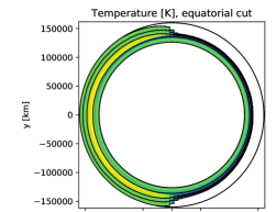
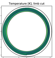
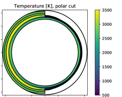
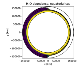
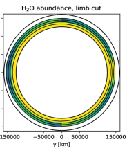
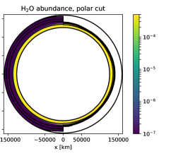
Figure 1: GCM simulation of Wasp-121b (Parmentier et al., 2018) without H₂ dissociation. Temperature (top) and the water abundance (bottom) for equatorial cut (left), limb cut (middle), and pole cut (right). From center outward, the 5 solid lines are respectively the $1,434.10^{7}$, $10^{3}$, 1, $10^{-2}$, and $10^{-4}$ Pa pressure levels. The colormap for water abundance maps goes from $5.10^{-4}$ to $10^{-7}$. Note that the radius of the planet and the atmosphere are shown to scale.

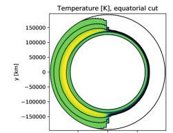
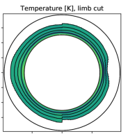
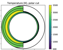
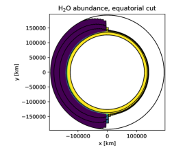
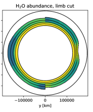
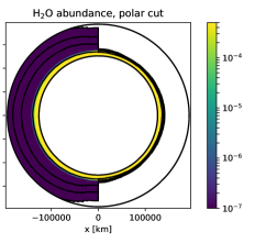
Figure 2: Same plots as Fig 1 but taking into account H₂dissociation. We clearly see that the dissociation of H₂ mostly affects the day side of the atmosphere which increases even more the dichotomy between the day and the night side.

2.2 Generation of transmission spectra with Pytmosph3R

Transmission spectra are computed using Pytmosph3R   as described in Caldas et al. (2019). Pytmosph3R is designed to simulate transmission spectra based on any 3D atmospheric structure, including outputs of a Global Circulation Model (GCM ). It produces transmittance maps at any wavelength that can later be spatially integrated to yield the transmission spectrum. The code can account for molecular opacities using the correlated-k method (Fu & Liou, 1992) or monochromatic cross-sections calculated by ExoMol (Yurchenko et al., 2011; Tennyson & Yurchenko, 2012; Barton et al., 2013; Yurchenko et al., 2014; Barton et al., 2014). In this study, we only use the latter to ensure a complete compatibility with the TauREx retrieval code (Waldmann et al., 2015b, a). Unless stated otherwise, our simulations only include H₂, He, H₂O, and CO. We also take into account H₂-H₂  and He-H₂  continua and the atmospheric scattering. To simplify the analysis, we did not include TiO and VO to focus on the molecules above.

The abundances of the species in the atmosphere are calculated based on the temperature given by the GCM simulation and following Parmentier et al. (2018) when dissociation occurs as described in Sect 2.1. The molecular weight then derives from these abundances. The gravity and the atmospheric scale height vary with the altitude from the planetary surface, i.e. the radius of the planet at a pressure of 10 bar, as described in Caldas et al. (2019), and are defined, respectively, in Eq (1) and (2):

$$g(z)=g_{0}\frac{1}{\left(1\,+\,\frac{z}{R_{p}}\right)^{2}}$$ (1)

$$H(z)=\frac{kT(z)}{\mu(z)g(z)},$$ (2)

where $g_{0}$ is the surface gravity, $R_{p}$ is the planetary radius, $T$ is the temperature and $\mu$ is the mean molecular mass.

We define the volume mixing ratio (VMR) as:

$$x_{\mathrm{i}}=\frac{N_{\mathrm{i}}}{\sum{N_{\mathrm{i}}}},$$ (3)

where $N_{\mathrm{i}}$ is the molecular number density in molecules per volume unit. We also assume that all the others species are present in the atmosphere as trace gases, so we can write the number density of atomic Hydrogen:

$$N_{\mathrm{H}}=2\left(N_{\mathrm{H_{2}}}^{0}\,-\,N_{\mathrm{H_{2}}}\right)$$ (4)

where $N_{H_{2}}^{0}$ is the molecular number density when no dissociation occur – e.g. deep in the atmosphere (see Tab.  1).

We ran Pytmosph3R at R=10000 resolution, with $R=\frac{\lambda}{\Delta\lambda}$, in the spectral range from 0.6$\,\mu$m to 10$\,\mu$m. The spectra are then binned down to a resolution of R=100 for the retrievals. We use this low spectral resolution for several reasons:

1. We simulate JWST observations from 0.6 to 10 $\mu$m using the low resolution prism mod provided by Near Infrared Spectrograph (NIRSpec) and Mid Infra-Red Instrument (MIRI) instruments (Stevenson et al., 2016). This does not entail that using the prism configuration is the best observational strategy for such a bright target, but provides us with a uniformly sampled spectrum that does not arbitrarily put more weight in the retrieval on some spectral regions;

2. We compared TauREx with the fully homogeneous case planet, as in Caldas et al. (2019), and we saw that the optimum resolution for the best accuracy in the retrieval is the resolution R=100.

3. There are only two absorbing species in our atmosphere (H₂O and CO) and we do not need to resolve specific lines, but large features in large spectral bands;

In all our simulations we used the planetary and stellar parameters shown in Tab  2. In the part of the atmosphere where H₂ does not dissociate, we have a fixed $\frac{He}{H_{2}}$ ratio at 0.25885. Then, we compute the volume mixing ratios of H and He by combining the equations (3) and (4) where H₂ dissociates.

Since the overall flux is dominated by the star, we assume that the spectral noise is dominated by the stellar photon noise, defined as:

$$N_{\mathrm{phot}}=\frac{\pi\tau\Delta t}{hc}\left(\frac{R_{*}D}{2d}\right)^{2}\int_{\lambda_{1}}^{\lambda_{2}}B(\lambda,T_{*})\lambda d\lambda,$$ (5)

where $\lambda_{1}$ and $\lambda_{2}$ are the limiting wavelengths of the bin considered, $d$ is the distance of the star (270 pc for WASP-121) and $R_{*}$, $T_{*}$ are, respectively, the stellar radius and the effective temperature. $D$, $\tau$ and $\Delta t$ are, respectively, the telescope diameter, the system throughput and the integration time, whose values has been fixed for JWST according to Cowan et al. (2015).

Using Eq 5, the uncertainty varies from 10ppm to 50ppm between 1 and 10$\mu$m, assuming a single WASP-121b transit. Since systematics may prevent us from reaching a 10ppm precision with JWST, wherever the shot noise was lower than 30ppm we assumed a floor noise of 30ppms through the whole spectral domain (Greene et al., 2016).

Note that we compute different 3D structures as input for Pytmosph3R with the parameters described in table  1. We will describe in details those structures in section 3.

Input parameters	Min-Max temperature [K]	angle $\beta$	$P_{\mathrm{bot}}$ [Pa]	$P_{\mathrm{top}}$ [Pa]	$x_{\mathrm{CO}}$ [log(VMR)]
Symmetric case $\nabla^{-}T$	1400-2800	20°	$10^{6}$	$10^{-4}$	-3.36
Symmetric case $\nabla^{+}T$	500-3500	10°	$10^{6}$	$10^{-4}$	-3.36
GCM case	493-3545	-	$1.434\times 10^{7}$	$10^{-4}$	-3.36

Table 1: Parameters used in the three simulation configurations of WASP-121b.

Star	Mass [$M_{\mathrm{S}}$]	Radius [$R_{\mathrm{S}}$]	Temperature [K]	Bibliographical references
Wasp-121	1.353	1.458	6460	Delrez et al. (2016)

Planet	Mass [$M_{\mathrm{J}}$]	Radius [$R_{\mathrm{J}}$]	Temperature [K]	Bibliographical references
Wasp-121 b	1.183	1.8	2360	Delrez et al. (2016), Evans et al. (2016)

Table 2: Mass, radius and temperature parameters of the WASP-121 star (top) and its planet Wasp-121 b (bottom). They are used both for the observable generations and the retrievals.

2.3 Retrieval model: TauREx

The spectral retrievals has been computed with the TauREx retrieval code (Waldmann et al., 2015b, a). TauREx consists in a Bayesian retrieval code which uses the ExoMol line lists (Yurchenko et al., 2011; Tennyson & Yurchenko, 2012; Barton et al., 2013; Yurchenko et al., 2014; Barton et al., 2014), HITRAN (Rothman et al., 2009; Gordon et al., 2013) and HITEMP (Gordon et al., 2010). TauREx assumes a plane parallel exoplanetary atmosphere with a one-dimensional distribution elements and temperature-pressure profile. We assume the radius at the base of the model of Wasp-121b as the value for which the atmospheric pressure is 10 bar. We simulate the exoplanetary atmosphere assuming a pressure between $10^{6}$ and $10^{-4}$ Pascals. We consider an atmosphere dominated by Hydrogen and Helium, with a mean molecular weight of 2.3 amu. We also suppose the presence of CO and H₂O as trace gases.

An important assumption is that TauREx does not take into account thermal dissociation of species and assumes the molecular abundances constant with the atmospheric pressure (see Changeat et al. (2019) for a detailed discussion on the effect of this assumption). We set up the prior range for the molecular volume mixing ratios of CO and H₂O between $10^{-12}$ and $10^{-1}$ which allow us to explore a large range of solutions. Even if we never add clouds in our input simulation, we set up the prior range for clouds between $10^{-12}$ and $10^{-1}$ to allow the retrieval code to have more freedom. We also feel that this better simulates a real situation where clouds would be put in the retrieval without prior knowledge about their occurrence in the real planet. The allowed range for the planetary radius and the atmospheric temperature (assumed constant in the vertical) are, respectively, $1.3R_{Jup}-4.0R_{Jup}$ and $400K-3600K$, with $R_{Jup}$ the radius of Jupiter. The range for the temperature is linked to the minimal and maximal temperature in the GCM simulation of Wasp-121b   as shown in Tab 1. As we simulate JWST observations, we set up the range of wavelength between 0.6 to 10 $\mu$m. For the non-retrieved parameters such as masses and stellar radius, we use those describe in Tab 2.

We note that the TauREx retrieval code is not designed to take into account the thermal dissociation of H₂. When H₂ thermal dissociation occurs, the He/H₂ ratio changes as a function of pressure and temperature. The mean atmospheric weight can also be lower than 2amu. In order to be consistent across all our sets of simulations, we used the same configuration file for our spectral retrievals and we left the He/H₂ ratio constant. By doing so we could estimate whether an atmosphere where H₂ dissociation does not occur can explain our input spectrum or not. We will come back to this in the Sect 4.2.3.

Again, some of these assumptions may seem too simplistic in view of the physics we envision in the real atmospheres of UHJs, but we think that it is important to understand how such simplistic assumptions – commonly used nowadays – can bias the conclusions from a retrieval analysis.

3 Input models: from simple case to GCM simulations

In order to understand and to characterize the biases due to the atmospheric 3D structure of Wasp-121b atmosphere, we decided to start from a simple case, and add, as the study progresses, further levels of complexity. Using this approach, we will show how to distinguish the observed biases. Note that we used the same atmospheric composition in all our cases, which is He, H₂, H₂O and CO.

The validation of Pytmosph3R ’s model with TauREx was done by Caldas et al. (2019). So, we started by considering the atmospheric 3D structure of an idealized Wasp-121b . In Figs 3 and 4 we show the 3D temperature maps used by Pytmosph3R to calculate the transmission spectrum. With this model we neglect effects which depend on the altitude, using isothermal pressure-temperature profiles in each cell, and we focus on the compositional effects. Finally, we simulated a 3D atmospheric structure of Wasp-121b using a Global Circulation Model (GCM) which takes into account both vertical and horizontal effects.

3.1 Idealized 3D atmosphere with day to night gradient

3.1.1 Effects of the day-night temperature gradient

First, we create an idealized case of Wasp-121b atmospheric structure that is symmetric around the planet/observer line of sight. The main parameters to simulate this simple structure are $T_{\mathrm{d}}$ and $T_{\mathrm{n}}$ and $\beta$, respectively the day-side, the night-side and the opening angle. $T_{\mathrm{d}}$ and $T_{\mathrm{n}}$ are correlated respectively to the sub-stellar and the anti-stellar point. The opening angle $\beta$ describes how the transitions between the day and the night side is computed, the smaller the sharper. We constructed our model by going symmetrically from the day side to the night side temperature considering a linear transition between the two. To avoid as much as possible effects due to vertical temperature gradients, every column of our model follows an isothermal profile above a given pressure level ($P_{\mathrm{iso}}=0.13\,\mathrm{bar}$). In this part of the atmosphere, the temperature however varies with respect to the local solar elevation angle, $\alpha_{*}$. In the deeper parts of the model, in accordance with results from a GCM for Wasp-121b (see Sect. 2.1), the temperature is uniform and set to 2500 K. In summary, for a given pressure and local solar elevation angle, the temperature is given by:

$$\left\{\begin{array}[]{rl}P>P_{\mathrm{iso}}&T=T_{\mathrm{d}}\\ P<P_{\mathrm{iso}}&\left\{\begin{array}[]{rl}2\alpha_{*}>\beta&T=T_{\mathrm{d}}\\ \beta>2\alpha_{*}>-\beta&T=T_{\mathrm{n}}+(T_{\mathrm{d}}-T_{\mathrm{n}})\frac{\alpha_{*}+\frac{\beta}{2}}{\beta}\\ 2\alpha_{*}<-\beta&T=T_{\mathrm{n}}\end{array}\right.\end{array}\right.$$ (6)

For Wasp-121b we considered two end-member cases:

1. The high gradient model ($\nabla^{+}T$ ), which goes from $500\,\mathrm{K}$ to $3500\,\mathrm{K}$ using $\beta=10^{\circ}$. This one is supposed to be representative of the day-night gradient present in the GCM without the heterogeneities in the vertical direction and along the limb.

2. The low gradient model ($\nabla^{-}T$ ), which goes from $1400\,\mathrm{K}$ to $2800\,\mathrm{K}$ using $\beta=20^{\circ}$. This case is more representative of GCM simulations accounting for the thermal effect of H₂recombination. We anticipate this case to be conservative and to provide a lower bound for the real bias caused by day-night temperature differences.

Fig. 3 and Fig. 4 show the temperature structure of the atmosphere of the cases studied. These maps are plotted to scale. Note that we consider a symmetric atmospheric structure, so the equatorial cut and the polar cut are exactly the same. As we can see, the day side of those atmospheres are strongly inflated in comparison to the night side which will create the horizontal biases that we want to characterize.

The $\nabla^{+}T$ and $\nabla^{-}T$ cases have been chosen to encompass the real day-night gradient present in Wasp-121b (see below) while removing effects due to differences along the limb (for example, east vs. west limb or equator vs. poles). This should allow us to identify the specific effect of these differences by comparing the retrieval results with our idealized cases and with the actual GCM outputs.

The $\nabla^{+}T$ case is close to the GCM case. Bell & Cowan (2018) and Tan & Komacek (2019) showed that the energy redistribution effect of hydrogen recombination cools the day side, heats the night side and reduces the gradient across the limb. The $\nabla^{-}T$ case thus uses a reduced gradient to account for this effect and present a very conservative estimate of the 3D effect.

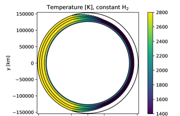
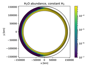
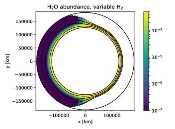
Figure 3: Atmospheric structure of the symmetric, idealized case $\nabla^{-}T$ , assuming an absence and the presence of H₂ dissociation (left and right respectively). We show the temperature map (top) and the water abundance map (bottom). The temperature gradient goes from $\mathrm{1400\,K}$ to $\mathrm{2800\,K}$. The transmission angle is 20° around the terminator line and have a $\mathrm{2500\,K}$ ring at P=$\mathrm{0.13\,bar}$ from the surface pressure. From center outward, the 5 solid lines are, respectively, the $10^{6}$, $10^{3}$, 1, $10^{-2}$, and $10^{-4}$ Pa pressure levels. The colormap for water abundance maps goes from $5.10^{-4}$ to $10^{-7}$. Note that the radius of the planet and the atmosphere are shown to scale.

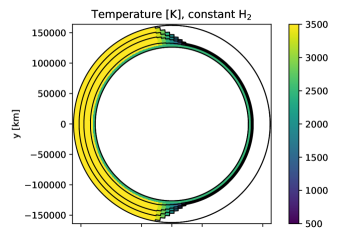
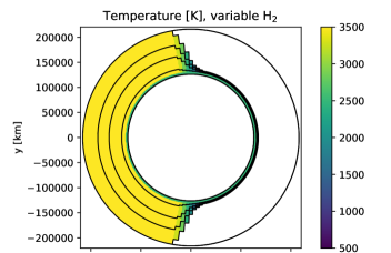
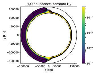
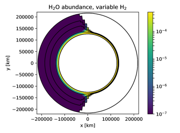
Figure 4: Atmospheric structure of the symmetric, idealized case $\nabla^{+}T$ , assuming an absence of H₂ dissociation. We show the temperature map (top) and the water abundance map (bottom). The temperature gradient goes from $\mathrm{500\,K}$ to $\mathrm{3500\,K}$. The transmission angle is 10° around the terminator line and have a $\mathrm{2500\,K}$ ring at P=$\mathrm{0.13\,bar}$ from the surface pressure. From center outward, the 5 solid lines are, respectively, the $10^{6}$, $10^{3}$, 1, $10^{-2}$, and $10^{-4}$ Pa pressure levels. The colormap for water abundance maps goes from $5.10^{-4}$ to $10^{-7}$. Note that the radius of the planet and the atmosphere are shown to scale. The temperature and abundance maps of the $\nabla^{-}T$ case are almost the same with only a smaller scale height of the atmosphere.

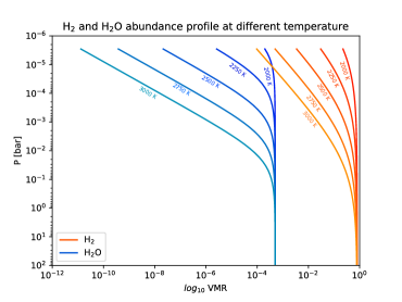
Figure 5: H₂O and H₂ abundance profiles plotted for a range of temperature between 2000 K and 3000 K. At a given pressure, H₂O and H₂ dissociation depends strongly on the temperature. The higher the temperature, the lower the abundance in the atmosphere. At a fixed temperature, the variation of the dissociation rate depend as a function of P and $\mathrm{P}^{2}$, respectively, for H₂ and H₂O.

3.1.2 Composition effects due to the dissociation of some molecules

In UHJs, molecular abundances are not the same everywhere, since the day-side temperature is high enough to allow thermal dissociation of many species (Lodders & Fegley, 2002; Visscher et al., 2006, 2010; Marley et al., 2017). In this work, we take into account the dissociation of two molecular species, first only H₂O and later also H₂, using the equations provided by Parmentier et al. (2018) as shown in Fig. 5. At a given temperature, the lower the pressure, the stronger the dissociation and at a given pressure, higher the temperature higher the dissociation. In this study, we assume that dissociated H₂ predominantly forms atomic hydrogen. We know that hydrogen anion can absorb part of the electromagnetic radiation between 1$\mu$m and 10$\mu$m (Lenzuni et al., 1991; Parmentier et al., 2018). However, we did not include in our computations the absorption contribution from ionized hydrogen. The main reason is that we want to be consistent with TauREx, which does not include this opacity source. Furthermore, the dissociation of CO  cannot occur at the temperature regimes in our simulations, i.e. 500K to 3500K. In order to dissociate, CO  requires higher temperatures, due to its stronger triple bond (Lodders & Fegley, 2002). For this reason, we assumed in all the simulations, a constant CO  abundance everywhere in the atmosphere. In the first set of simulations, we considered the $\nabla^{+}T$ and $\nabla^{-}T$ models considering water dissociation alone (H₂ is held constant). As shown in the abundance map of H₂O in Figs. 3 and 4, there is no more water in the day-side of the planet at pressure lower than $P_{\mathrm{iso}}$. The dissociation stops around the terminator and, in the night-side, the water distribution comes back at a constant value.

In the second set of simulations we took into account both H₂ and H₂O dissociation. As H₂ does not have significant absorption bands in the 0.6 - 10$\mu$m wavelength range, the main effects of its dissociation is to decrease the molecular weight, causing an increase of the atmospheric scale height. It also affects the thermochemical properties of the atmosphere because atomic hydrogen recombines on the night side. This redistribution of energy will heat the night side and cool the day side (Bell & Cowan, 2018; Tan & Komacek, 2019). An other important effect is that without H₂ in the atmosphere, collision induced effects from both, H₂-H₂  and He-H₂  collisions, are less significant. As shown in Figs. 3 and 4, H₂  dissociation increases the atmospheric scale height of the day side by a factor of 1.5 and 2 in the $\nabla^{-}T$ and $\nabla^{+}T$ simulations, respectively. We note that, the temperature is not high enough to induce H₂ dissociation in the night side. This characteristics, creates an even stronger difference between the night side and the day side when H₂ dissociates. Consequently, CO is the dominant radiatively active species in the day-side because it does not dissociate at these temperatures.

3.2 3D models of Wasp-121b atmosphere using SPARC/MITgcm global circulation model

In the last configuration, we add both the vertical and azimuthal (along the limb) effects. Indeed, we model Wasp-121b using the Global Circulation Model (GCM) SPARC/MITgcm Parmentier et al. (2018) described in Sect 2.1. The chemistry is kept unchanged. As in Sect. 3.1, we studied four different cases considering all the possible combinations where water and H₂  dissociate. Figs. 1 and 2 show the temperature and water abundance maps for the GCM cases with and without H₂ dissociation. We see that the thermal structure of the atmosphere is more complex than the one in the symmetric case, even if the salient features remain the same. The most important modification concerns the terminator which is now asymmetric because of the winds created by the strong temperature dichotomy between the day and night side (Showman et al., 2015). Those equatorial jets warm the east side of the atmosphere and cools the west side around the equator, which implies less dissociation of water on the west because of the cooler temperature. Nevertheless, the abundance maps show that there is still water dissociated at the terminator which could allow the light to probe deeper into the atmosphere on the night side of the planet. Note also that when H₂ dissociation is taken into account, the global behavior of the 3D structure remains the same, but since the day side of the atmosphere has a bigger scale height, it is more inflated.

An important caveat here is that while we model H₂ dissociation to compute the transit spectrum, the dissociation is not taken into account in the GCM itself. This is expected to reduce the day night contrast thus the winds fields (Bell & Cowan, 2018; Tan & Komacek, 2019). So this case is not completely self consistent.

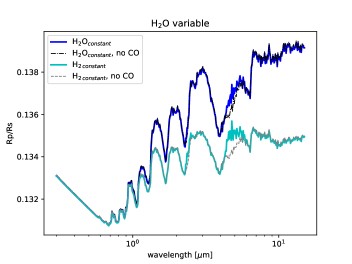
(a)

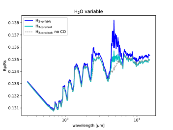
(b)

Figure 6: (Left): Transmission spectra of Wasp-121b at resolution of R = 100 for GCM simulations assuming a constant H₂abundance in the whole atmosphere. When water dissociation is taken into account (light blue line), the water features become shallower compared to when we assume no water dissociation (blue line). (Right): Transmission spectra of Wasp-121b at resolution of R = 100 for GCM simulations taking into account H₂Odissociation in the atmosphere. When H₂ dissociation is considered (blue line), the CO features appears more clearly compared to when we neglect H₂ dissociation (light blue line). Black line and grey line correspond to the transmission spectra for an atmosphere without CO for the water constant and dissociated case respectively to highlights the features of CO in the other curves.

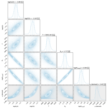
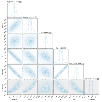
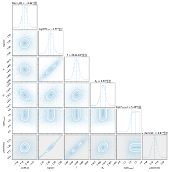
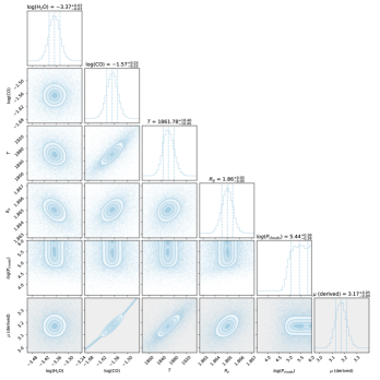
Figure 7: Nest posteriors retrieval from TauREx assuming a constant H₂ abundance in the atmosphere. There are the $\nabla^{+}T$ (left) and GCM cases (right) which assume, respectively, no water dissociation (Top) and water dissociation (Bottom). We retrieved five free parameters which are H₂O, CO abundances in log10(VMR), clouds pressure in bar, the temperature in Kelvin and the planetary radius in Jupiter’s radius. The molecular weight is derived from those parameters.

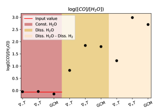
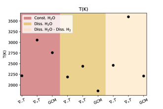
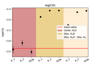
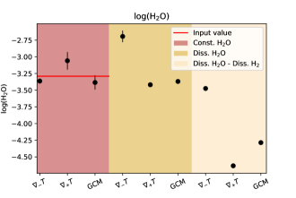
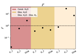
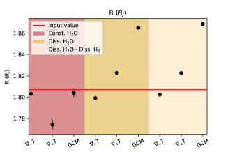
Figure 8: Summary of all the retrieval results for $\nabla^{-}T$ , $\nabla^{+}T$ and GCM simulation considering every cases. We show the $[\mathrm{CO}]/[\mathrm{H}_{2}\mathrm{O}]$ ratio (top left), the temperature (top right), the log abundances of CO (middle left) and H₂O (middle right), the $\tilde{\chi}^{2}$ (bottom left) and the planetary radius (bottom right). Those retrievals have been calculated with a shot noise assuming a floor noise of 30ppms through the whole spectral domain. The red line represents the input value from our simulations and the black dot line shows where the $\tilde{\chi}^{2}$=1.

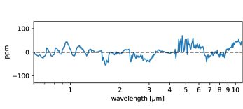
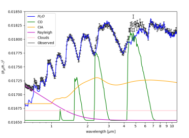
Figure 9: Particular solutions found by TauREx in the GCM case assuming water dissociation and H₂ constant. In the bottom: we show the contribution plots of each component, i.e. H₂O, CO and Collision Induced Absorption (CIA) for the solution found by TauREx. In the top: residuals (in ppm) between the input spectrum and the best-fit spectrum.

4 Results

In this section, we describe the results of the transmission spectra generated by Pytmosph3R and the spectral retrieval using our three set of simulations, each one being performed on our three temperature structures ($\nabla^{-}T$ , $\nabla^{+}T$ , and GCM):

1. H₂ and H₂O constant in the whole atmosphere;

2. Thermal dissociation of H₂O with H₂ held constant;

3. Thermal dissociation of both H₂O and H₂.

4.1 The 3D transmission spectrum of ultra hot Jupiters

The transmission spectra generated by Pytmosph3R are shown in Fig. 6. Here, we tested two cases with H₂ constant considering or not water dissociation in the atmosphere (Fig. 6a), and a third one with both H₂O and H₂ dissociation (Fig. 6b). When H₂O is constant, the water features are more evident and the CO’s features are barely visible as it is highlighted comparing the transmission spectra with and without CO in the atmosphere (respectively the blue and the dotted black lines). Since there is CO and H₂O everywhere, then the transmitted light probes the same region for both molecules, which are at a high altitude in the day side of the atmosphere. In this case then the spectral features are similar to the ones of the 1D case.

When H₂O dissociates (light blue curve in Fig. 6a), the water features in the spectrum become smaller because it almost disappears from the day side of the atmosphere. Then, the light from the star can probe much deeper regions of the atmosphere in the wavelength range where the CO does not absorb and reaches part of the night side. The CO, which is not dissociated on the day side - where the scale height is large due to the high temperature - appears more evidently. So, as the light goes first through the day side and then through the night side, the transmission spectrum carries information of both sides of the atmosphere depending on the wavelength we look at. The behavior of the spectrum can also be understood looking at Figs. 1 and 4 where the maps of the atmosphere show the lack of water in the day side except for a deep part of the atmosphere ($\simeq\,$10 mbar). Since CO does not dissociate, it absorbs mainly in the day-side of the atmosphere, where the high temperature leads to larger absorption features.

When both H₂O and H₂ dissociate, the water features are similar in both presence and absence of H₂ dissociation as shown in Fig 5 and Fig 6b. Indeed, the main effect of the dissociation of H₂ in the atmosphere is the increasing of the scale height. As the dissociation of H₂ mainly occurs in the day side of the atmosphere as well as the dissociation of H₂O (see Fig 1 and 2) the region probed is the same in both cases. However, the CO features appears even more clearly. As CO abundance remains constant everywhere in the atmosphere, its features are more significant due to the enlarger of the scale height caused by the dissociation of H₂ in the day side.

Note that Fig. 6 represents the transmission spectra for the case with the GCM input, but the whole behaviours explained above remain similar to the symmetric $\nabla^{+}T$ and $\nabla^{-}T$ cases.

4.2 Retrieval results

4.2.1 H₂ and H₂O constant in the atmosphere

The posterior distributions of $\nabla^{+}T$ and GCM simulations are shown in Fig 7. The retrieval code TauREx converges, in every simulation, to a non-degenerate solution. Fig. 8 summarizes all the solutions found by TauREx for each simulation. As shown in the red part of the various panels of this figure, TauREx finds non-degenerate solution within 2$\sigma$ from the input H₂O and CO abundance for the $\nabla^{+}T$ , $\nabla^{-}T$ and GCM simulations. Those chemically homogeneous simulations are similar to what Caldas et al. (2019) have done, that’s why we expected to find consistent results with their work. To better interpret those results, we plotted the $[\mathrm{CO}]/[\mathrm{H}_{2}\mathrm{O}]$ ratio (Fig 8). This ratio allows us to understand if the dissociation of water affects the spectrum. The $[\mathrm{CO}]/[\mathrm{H}_{2}\mathrm{O}]$ ratio is constant when water does not dissociate, which it is found here by TauREx retrieval. The temperatures retrieved suggest that the light is probing the day side of the atmosphere. Indeed, as shown in Fig 4 and Fig 1, the atmosphere presents an inflated day side. The temperature retrieved in the $\nabla^{+}T$ case is higher than the one retrieved in the $\nabla^{-}T$ case which is expected since the temperature of the day side are higher in the $\nabla^{+}T$ case. Using as input the spectrum computed with GCM, TauREx finds a slightly lower temperature than the one found in the two symmetric simulations. Considering that the GCM simulations has been made assuming a non-isothermal temperature-pressure profile, the temperature structure of GCM is indeed more complex than the one in the other two simulations. These results are all consistent with Caldas et al. (2019). Note that the calculated $\chi^{2}$ is much higher for the GCM case compared to the symmetric cases $\nabla^{+}T$ and $\nabla^{-}T$ .

4.2.2 Thermal dissociation of H₂O with H₂ constant

When water dissociation is taken into account, TauREx returns significantly different solutions compared to the homogeneous simulations. The results are shown in the yellow parts of Fig. 8.

First, all the retrieved temperatures are lower than the ones found in the constant composition simulations. Because the main constraint that allows TauREx to retrieve the temperature is the amplitude of the spectral bands - the higher the temperature the higher the amplitude - the temperatures retrieved are lower because the water features are coming from a colder region of the atmosphere. In the GCM case, the temperature retrieved is lower than the temperatures of the limb, which suggest that we probe the night side of the atmosphere.

Since CO does not dissociate, it absorbs mainly in the day-side of the atmosphere, where the high temperature leads to larger absorption features as explained in Sect 4.1. Looking at the yellow part of Fig 8, there are non-degenerate solution for TauREx to fit the CO features, considering that it also finds a low temperature because of the presence of water in the cold night-side of the planet. This solution suggests a high CO abundance in the atmosphere and converges around the correct water abundance within 3$\,\sigma$. This water abundance corresponds indeed to the abundance in the night side of the atmosphere where water is not dissociated (see Figs 1, 3 and 4).

As a consequence, the $[\mathrm{CO}]/[\mathrm{H}_{2}\mathrm{O}]$ is around 100 times higher than expected. We note that for the conservative case $\nabla^{-}T$   the $[\mathrm{CO}]/[\mathrm{H}_{2}\mathrm{O}]$ is less biased, around 10 times higher than the solar abundance, due to the smaller day to night contrast and the smoother transition between them. To quantify the reliability of the solutions given by TauREx , we plotted the absorption contribution plots of the solutions for the GCM case and the differences in ppm between the generated and the retrieved spectrum in Fig 9. We highlight here in which wavelength bands the fit is good or not. Moreover, the calculated $\tilde{\chi}^{2}$ which is below 1 for each simulation, demonstrates a high significance level of the solution given by TauREx (see Fig 8).

4.2.3 Thermal dissociation of H₂ and H₂O

In Fig 8 we give the $\tilde{\chi}^{2}$ values for each simulations. We see that TauREx finds non-degenerate solution for every simulation, although they are not all statistically significant, i.e. $\tilde{\chi}^{2}$$\,\gg\,1$ in $\nabla^{+}T$ and GCM cases. In the previous cases where we have a constant composition in the entire atmosphere and in the case where only water dissociates in the day side, TauREx finds a consistent solution, even though it does not necessarily converge towards the correct input parameters. On the contrary, when H₂ dissociation is taken into account, TauREx cannot find a suitable solution to explain the atmospheric spectrum. As shown in the lower left panel of Fig. 8, the best reduced $\chi^{2}$ for in $\nabla^{+}T$ and GCM models with H₂ dissociation are respectively around 30 and 8. The $\chi^{2}$ test can give us a possible signal that in the planet we are taking into account it occurs H₂ dissociation. However, TauREx manages to find statistically significant solution in the $\nabla^{-}T$ case, but we keep in mind that this simulation is a conservative choice and we think that the truth remains in between $\nabla^{-}T$ and $\nabla^{+}T$ simulations.

We note that the TauREx retrieval code is not designed to take into account the thermal dissociation of H₂. When H₂ dissociation occurs, the He/H₂ ratio changes as a function of pressure and temperature. The mean atmospheric weight can also be lower than 2amu in the atmospheric regions where H₂ dissociates. In order to be consistent with all the set of simulations, we used the same configuration file for our spectral retrievals and we left the He/H₂ ratio constant. By doing so we could estimate whether an atmosphere where H₂ dissociation does not occur can explain our input spectrum or not.

The H₂ dissociation plays a major role on the spectra and the retrievals results. All the results are shown in the light yellow part of Fig 8. In each simulation, the $[\mathrm{CO}]/[\mathrm{H}_{2}\mathrm{O}]$ ratio retrieved is higher than the one calculated when H₂ is constant. As CO abundance remains constant everywhere, its features are, then, more significant as explained in Sect. 4.1 and TauREx finds a best fit model with a low water abundance and a high CO abundance. As a consequence, the $[\mathrm{CO}]/[\mathrm{H}_{2}\mathrm{O}]$ ratio increases.

As shown in the light yellow part in Fig 8, when we consider H₂ dissociation in the GCM case TauREx finds non-degenerate solution. The temperature retrieved is a bit higher than the temperature we find when H₂ does not dissociate. Indeed, as shown in Fig 6, H₂ dissociation does not alter the amplitude of the water features dramatically. This is because the water absorption comes from the cold night side of the planet where molecular H₂ dominates. Thus, the temperature retrieved still corresponds to the temperature of the night side.

For the other retrieved parameters, we are consistent with the solution found when H₂ is constant. We remember that the dissociation of H₂ affects the transmission spectrum in mainly 2 ways: i) it increases the scale height of the day side of the atmosphere implying stronger features for species who remains in the day side such as CO. We only consider this effect in the $\nabla^{+}T$ simulation; ii) it also significantly affects the thermochemical properties of the atmosphere due to the recombination of H₂ in the night side which redistribute the energy, heating the night side and cooling the day side (Bell & Cowan, 2018; Tan & Komacek, 2019). We took into account both of them in the $\nabla^{-}T$  simulation. H₂ dissociation results also in a decrease of $\mathrm{H}{{}_{2}}$-$\mathrm{H}{{}_{2}}$ and He-$\mathrm{H}{{}_{2}}$ collisions, hence less intense continuum absorptions. However, in the $\nabla^{+}T$ simulations, TauREx does not manage to converge to a reasonable solution. TauREx cannot explain the line distortion using a 1D atmospheric model and tends to increase the temperature far above the equilibrium temperature of the planet, reaching the upper prior range temperature, i.e. 3600K. (see Fig. 8).

When both H₂ and H₂O dissociate, it is not possible to find any 1D atmospheric model that matches with the input spectrum in any of the cases under study in this paper.

5 Discussions

Our results show that a 1D model is always able to find a statistically consistent solution – except for the case in which H₂ dissociation occurs – although it does not always converge towards the correct input solution.

Caldas et al. (2019) showed that day-night temperature contrasts lead to a bias in retrieved temperatures (toward the one of the day side) even when the chemical composition is uniform. In this work, we extend this by showing that when we take into account H₂O dissociation, we have both composition and temperature biases.

Although a retrieval code can use a 1D atmospheric model to detect the presence of a particular chemical species from an atmosphere with a complex 3D structure, measuring its abundance is more challenging. When temperature and chemical composition vary across the limb, the 1D retrieval cannot find the correct molecular abundances: the best fit parameters can be several orders of magnitude different from the correct input ones, as shown in Fig 8.

Elemental ratios (such as C/O, C/N, etc.) are a key parameter determining the chemical processes taking place in planetary atmospheres (Line et al., 2013; Oreshenko et al., 2017). At high temperature, Madhusudhan (2012); Espinoza et al. (2017) showed that the C/O ratio plays a major role in the atmospheric chemistry and non-solar values could explain observations for 6 hot Jupiters (XO-1b, CoRoT-2b, WASP-14b, WASP-19b, WASP-33b, and WASP-12b). However, these elemental ratios cannot be directly measured, and we have to rely on measuring the abundance of all molecules carrying the considered elements. In the case of the hot, hydrogen dominated atmospheres considered here, H₂O and CO are the main carriers of carbon and oxygen so that the $[\mathrm{CO}]/[\mathrm{H}_{2}\mathrm{O}]$ is commonly expected to provide reasonable constraints on the C/O ratio. Our study shows that using $[\mathrm{CO}]/[\mathrm{H}_{2}\mathrm{O}]$ to constrain the C/O ratio when dissociation is present is highly hazardous and that finding $[\mathrm{CO}]/[\mathrm{H_{2}O}]\gg 1$ should be seen as a sign of chemical heterogeneities in the atmosphere. We note that the same diagnostic could be applied to other species such as TiO or VO by calculating the retrieved $[\mathrm{CO}]/[\mathrm{TiO}]$ or $[\mathrm{CO}]/[\mathrm{VO}]$ ratio.

The fact that our retrieval results are consistent for both the GCM model and our more idealized models of WASP-121b where temperature is constant in the vertical and symmetric around the substellar point reveals that, for UHJs at least, the effect of thermal and compositional heterogeneities across the limb dominate over the vertical ones as well as the ones along the limb. Fixing an atmospheric configuration – i.e. in presence or not of H₂ and/or H₂O dissociation, corresponding to the red, dark yellow, and light yellow areas in Fig 8 – the retrieved $[\mathrm{CO}]/[\mathrm{H}_{2}\mathrm{O}]$ ratio for the $\nabla^{+}T$ , $\nabla^{-}T$ , and GCM simulations are almost the same. This result shows that the idealized cases capture the most salient features of the GCM simulation. The most important point is that the retrieved $[\mathrm{CO}]/[\mathrm{H}_{2}\mathrm{O}]$ ratio reaches its minimum value when molecular dissociation does not occur, increases by a factor 10-100 when H₂O dissociates, and by a factor 25-1000 when H₂ dissociates as well, irrespective of the details of the vertical structure of equator-to-pole thermal contrasts. This large scale in the $[\mathrm{CO}]/[\mathrm{H}_{2}\mathrm{O}]$ ratio retrieved are due to our idealized $\nabla^{+}T$ and $\nabla^{-}T$ simulations which represent extreme cases, thus they encompass the biases.

A general characteristics of our results is that, in all the cases under our study, we cannot converge around the ground truth parameters. When we study a transmission spectrum extracted from a 3D atmosphere even a high signal to noise spectrum does not allow you to know the real chemical distribution of elements with a retrieval code which uses a 1D atmospheric approximation.

A second aspect is that, with a $\tilde{\chi}^{2}$-test it is possible to understand whether there is some more complex physical phenomenon in the atmosphere under study. In our case, we see that a $\tilde{\chi}^{2}$$\,>1$ was due to the presence of H₂ dissociation in our atmosphere. From this point of view, a $\tilde{\chi}^{2}$-test can reveal whether there is an important physical phenomenon that we are not considering.

Note that a limitation of our study concerns the chemical components of the atmosphere. We only consider two absorber species, CO and H₂O, but we know that other species have been detected in Wasp-121b such as TiO or VO. Plus, we also know that we are hot enough to dissociate those species (Parmentier et al., 2018) which would add more complexity in the retrieval analysis.

6 Are there hints of 3D structures in real data?

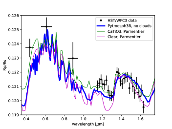
Figure 10: Transmission spectra of Wasp-121b at resolution of R = 100 for an atmosphere composed of He, H₂, H₂O, CO, TiO, VO, Na, Kand H^- using the analytical fit for the thermal dissociation of the species in Parmentier et al. (2018) (Blue). We compared the models with HST/WFC3 data taken from Evans et al. (2016) (black dot) and with two models from Parmentier et al. (2018), the first without clouds (magenta) and the second with CaTiO3 clouds (green).

In Fig. 10 we compare the spectrum of Wasp-121b as observed with HST/WFC3 (Evans et al., 2016) with two sets of synthetic transmission spectra: i) the models developed by Parmentier et al. (2018) that extract the columns at the terminator of their GCM simulation to compute the transmission spectrum, and ii) our models based on the same GCM simulation but with our more complete 3D radiative transfer framework. In addition to the radiatively active species discussed above, we account here for absoptions by TiO, VO, Na and H^- using the analytical fit for the thermal dissociation of the species in Parmentier et al. (2018). Compared to Parmentier et al. (2018), only FeH is missing, but it is believed to be less important in this part of the spectrum since we assume a solar composition.

In order to fit HST/WFC3 data, Parmentier et al. (2018) suggests to add CaTiO₃ clouds in the atmosphere to increase the absorption at 1.25 $\mu$m and fill the water window region. From our analysis, we see that considering a cloud free 3D structure can equivalently explain water amplitude in the WFC3 bandpass (thick blue line) even if our spectrum does not fit very good the data either. 3D effects can, indeed, deform the shape of the spectrum. The reason is however quite different. Instead of fitting the 1.25 $\mu$m window region, here the agreement is reached by reducing the strength of the 1.15 and 1.4 $\mu$m water bands thanks to water removal on the day side of the atmosphere. The fact that both models can have the same observed transit depth at these two wavelengths in Fig. 10 is just due to the fact that the radius at the base of the model remains a free parameter allowing us to shift the whole spectra vertically. Note that, expect for this parameter, there is no fitting of the abundances or thermal structure involved in our approach. We shown that because of the water dissociation, 3D effects was not negligible for atmospheres as hot as wasp-121b, even if clouds remains a reasonable assumption to fit the data. This findings suggests that both 3D heterogeneities in the transmission spectra and clouds can be combined to explain the reduction of the water feature. However, this is depending on which altitude the clouds remain and where they are in the atmosphere because even if there is clouds, the light rays could not probe them due to the 3D structure of the atmosphere.

7 Conclusion

The 3D structure of the planetary atmospheres plays a major role in shaping of the transmission spectra, especially for ultra hot Jupiters. The tidally locked planets have an inflated day side due to both the high temperature and the dissociation of species which increase the scale height of the day side atmosphere. In these atmospheres, the transmitted spectrum is affected by an extended region around the terminator line, which includes part of both the day side and the night side of the atmosphere.

The stellar light probes an atmospheric region which extends significantly toward the limb, depending on the chemical composition as a function of wavelength. If the temperature is not high enough to dissociate all the molecules, such as CO, they will remain everywhere in the atmosphere. Thus, the amplitude of their features in the transmission spectrum will be larger because they come from the hot regions if the inflated day side atmosphere. On the other hand, the molecules which dissociate more easily, such as H₂O, will only remain in the cold night side of the atmosphere. Therefore, the amplitude of the features of those molecules in the transmission spectrum will be less pronounced, since they come from colder regions in the night side of the atmosphere. A 1D retrieval code, which tries to fit the spectrum with an isothermal atmosphere, cannot unravel the information of a more complex temperature distribution and, then the abundances retrieved are biased. In particular, we demonstrate that for UHJs 1D retrieval would be biased towards high [CO]/[H₂O] ratio, the higher the ratio the stronger the chemical heterogeneities. For instance, the TauREx retrieval code finds the planetary temperature according to the strength of the main spectral features. Since the amplitude of the spectral features is rather large because of the gas present in the hot day side of the planet, it is natural for a retrieval code to converge towards hotter temperatures. In case of H₂O dissociation, the only relevant gas present in the hot day-side is the CO. The water absorption is due to the water present in the cold night side of the planet. Therefore, it is reasonable to retrieve a lower temperature in the case in which water dissociates in the day side.

We demonstrated that a three-dimensional atmospheric structure induces spectral distortions impossible to explain with a 1D retrieval. We also demonstrate that the water features can be strongly reduced by the presence of molecular heterogeneities due to a large day/night temperature contrast. For instance, we show that a 3D geometry can explain some of the features observed in the HST/WFC3 wavelength range of Wasp-121b , even in absence of hazes or clouds, thanks to the dissociation of water in the day side of the atmosphere. However, our works do not exclude the presence of clouds in UHJ atmospheres, the 3D effects are a complementary contribution to fill the water windows in the data. Thanks to our results, we think that Wasp-121b would be so a good target for future observations. We propose that 3D structural effects should already be consider when we study hot and ultra hot Jupiter to avoid erroneous conclusions. Moreover, future space missions such as JWST (Beichman et al., 2014) and ARIEL (Tinetti et al., 2018) will probe a very large range in wavelength (from 0.6 to 28 $\mu$m for JWST) and, then 3D effects will be even more evident in other parts of the exoplanetary spectra which has not been observed yet.

Finally, after the analysis of an exoplanetary atmosphere with a 1D retrieval tool, the $\tilde{\chi}^{2}$-test on a 1D retrieval can raise a warning about an important effect that the 1D model cannot consider, such as effects induced by the 3-dimensional structure of the exoplanetary atmosphere. In such cases, a parametrized 2D retrieval approach may be warranted. Whether there is enough information in the spectrum to actually constrain such a 2D approach remains to be demonstrated.