An empirical “high-confidence” candidate zone for $Fermi$ BL Lacertae Objects

Abstract

In the third catalog of active galactic nuclei detected by the $Fermi$ Large Area Telescope Clean (3LAC) sample, there are 402 blazars candidates of uncertain type (BCU). The proposed analysis will help to evaluate the potential optical classification flat spectrum radio quasars (FSRQs) versus BL Lacertae (BL Lacs) objects of BCUs, which can help to understand which is the most elusive class of blazar hidden in the Fermi sample. By studying the 3LAC sample, we found some critical values of $\gamma$-ray photon spectral index ($\Gamma_{\rm ph}$), variability index (VI) and radio flux (${\rm F_{R}}$) of the sources separate known FSRQs and BL Lac objects. We further utilize those values to defined an empirical “high-confidence” candidate zone that can be used to classify the BCUs. Within such a zone ($\Gamma_{\rm ph}<2.187$, log${\rm F_{R}}<2.258$ and ${\rm logVI<1.702}$), we found that 120 BCUs can be classified BL Lac candidates with a higher degree of confidence (with a misjudged rate $<1\%$). Our results suggest that an empirical “high confidence” diagnosis is possible to distinguish the BL Lacs from the Fermi observations based on only on the direct observational data of $\Gamma_{\rm ph}$, VI and ${\rm F_{R}}$.

March 6, 2019

1 Introduction

Blazars are a particular class of radio-loud active galactic nuclei (AGNs) with a relativistic jet pointing toward the Earth. The broadband (from radio up to TeV energies) emissions of blazars are mainly dominated by non-thermal components which are produced in the relativistic jet (Urry & Padovani, 1995). According to the strength of the optical spectral lines, blazars can be further divided into two subclasses (Stickel et al., 1991; Stocke et al., 1991; Laurent-Muehleisen et al., 1999), namely, the flat spectrum radio quasars (FSRQs; strong emission lines with equivalent width EW $\geq{\rm 5\AA}$ in rest frame) and the BL Lacerate objects (BL Lacs; weak or no emission and absorption lines). The multi-wavelength spectral energy distributions (SEDs) from the radio to $\gamma$-ray bands of normally exhibit a two-hump structure in the ${\rm log\nu-log\nu F_{\nu}}$ space. The low energy bump (peaking between millimeter and soft X-ray range) is always explained as synchrotron emission from the non-thermal electrons in the relativistic jet, while the high energy bump (peaking within MeV-GeV energy range) is inverse Compton (IC) scattering. Furthermore, based on the peak frequency ($\nu^{\rm S}_{\rm p}$) of the lower energy bump, blazars can also be classified as low- ( $\nu^{\rm S}_{\rm p}<10^{14}$ Hz), intermediate-( $10^{14}~{}\rm Hz<\nu^{\rm S}_{\rm p}<10^{15}$ Hz) and high-( $\nu^{\rm S}_{\rm p}>10^{15}$ Hz ) synchrotron-peaked sources (i.e., LSPs, ISPs, and HSPs, Abdo et al., 2010).

This work utilizes the third catalog of AGNs detected by the $Fermi$-LAT (3LAC) sample (Ackermann et al., 2015), which is part of the first four years of the $Fermi$-LAT data, the third $Fermi$ Large Area Telescope (LAT) source catalog (3FGL, Acero et al., 2015). The 3LAC clean sample (i.e., the high-confidence clean sample of the 3LAC) reports 1444 $\gamma$-ray AGNs: 414 FSRQs ($\sim$ 30%), 604 BL Lac objects ($\sim$ 40%), 402 blazar candidates of uncertain type (BCU, $\sim$ 30%) and 24 non-blazar type AGNs ($<$ 2%) (Ackermann et al., 2015). The identification of FSRQs and BL Lacs are solid, mostly based on the clear evidence on the (non-)existing of emission and/or absorption lines. On the other hand, BCUs are those sources without a confirmed classifications due to the missing representative features on optical spectrum (BCU I), synchrotron peak frequencies of SED (BCU II), and/or their broadband emissions (BCU III) (see Ackermann et al. 2015; Acero et al. 2015 for the details and references therein). Studying such a large sample of BCUs is crucial to understand of the physics of $\gamma$-ray emission of blazars (e.g., Singal et al. 2012; Singal 2015; Fan et al. 2016; Kang et al. 2018, 2019a, 2019b; Zhu et al. 2020).

Estimating the possible classification BL Lac vs FSRQ of BCUs can help to understand which is the most elusive class of blazar hidden in Fermi sample (Massaro et al. 2015). Indeed, some potential BL Lac or FSRQ candidates can be identified from the BCUs sample in the 2FGL/3FGL catalogues using different approaches such as supervised machine learning (e.g., support vector machine [SVM] and random forest [RF]; Hassan et al. (2013)), neural network (Chiaro et al., 2016), artificial neural network (ANN; Salvetti et al., 2017), multivariate classification method (Lefaucheur & Pita, 2017), and by statisical analysis of the broadband spectral properties (including spectral indices in the gamma-ray, X-ray, optical, and radio bands; Yi et al., 2017). In addition, we’ve identified potential BL Lacs and FSRQs candidates from the 3LAC Clean sample using 4 different SML algorithms (Mclust Gaussian finite mixture models, Decision trees, RF, and SVM; Kang et al. 2019a [Paper I]) and from the 4FGL catalogue using 3 different SML algorithms (ANN, RF, and SVM; Kang et al. 2019b). Nevertheless, the final confirmation of the BCU nature of candidates in all above approaches is subject to the observations of optical spectroscopy or counterparts in other wavelength (e.g., Massaro et al. 2014; Álvarez Crespo et al. 2016a, b, c; Massaro et al. 2016; Marchesini et al. 2016; Klindt et al. 2017; Peña-Herazo et al. 2017; Marchesi et al. 2018; Desai et al. 2019; Marchesini et al. 2019; Peña-Herazo et al. 2019), or broadband spectral features (e.g., Fermi/LAT collaboration, Massaro et al. 2009, 2012, 2016; Álvarez Crespo et al. 2016a, b, c). If such information is missing, classification of BCUs will become challenging especially when no training set is available (see e.g., Shaw et al. 2013; Landoni et al. 2015; Ricci et al. 2015; Paiano et al. 2017a, b; Landoni et al. 2018; Kaur et al. 2019; Kaur et al. 2019). To overcome such difficulties, in this letter, we aim to evaluate the potential classification of BCUs based on only on the direct observational properties in $\gamma$-ray and radio band. Such properties include $\gamma$-ray photon spectral index ($\Gamma_{\rm ph}$), and variability index (VI) and radio flux (${\rm F_{R}}$). By perform some detailed analysis, we confirmed the existence of a high-confident zone where the condition-met BCUs are most likely BL Lac objects.

We organize the present paper as follows. In Section 2, a brief description on the sample selection is provided followed by the proposed analysis methods and results. Comparisons of between our results with some other recent results are presented in Section 3. Our results are discussed in Section 4 and summarized in Section 5.

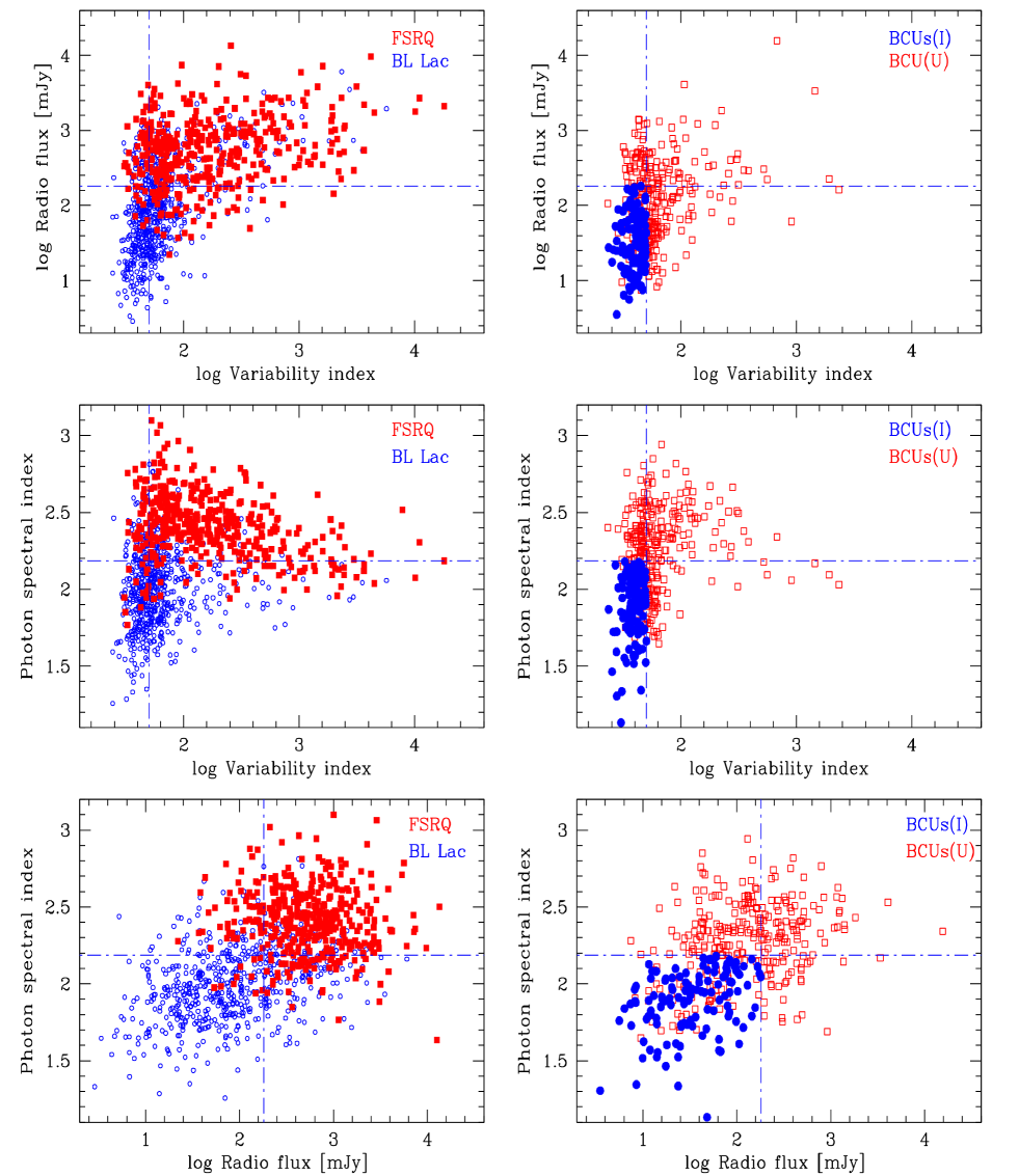
Figure 1: (Color online) The scatterplots of the variability index (VI), radio flux (${\rm F_{R}}$) and photon spectral Index ($\Gamma_{\rm ph}$) for fermi blazars (left column), where red solid squares represent FSRQs and blue empty points represent BL Lacs. The right panels represents the scatterplots of the BCUs (right column), where the BCUs (I) — are the identified BL Lacs (blue solid points) using the “$a_{i}<X$ zone” and the BCUs (U) — are the unidentified BCUs (red empty squares). The dotted-dashed parallel and perpendicular blue lines indicate $\Gamma_{\rm ph}$, log${\rm F_{R}}$, and log${\rm VI}$ is equal to 2.187, 2.258, and 1.702, respectively.

Table 1: The result of Two-sample Test

	Using	KS test			t-test				Wilcoxon-test
test dataset	Paramaters	$D$	$p_{1}$		$t$	df	$p_{2}$		$W$	$p_{3}$
	$\Gamma_{\rm ph}$, ${\rm logVI}$, log${\rm F_{R}}$	0.514	0		32	2455	$<$1.0E-6		1826100	$<$1.0E-6
604 BL Lacs	$\Gamma_{\rm ph}$, log${\rm F_{R}}$	0.587	0		31	1915	$<$1.0E-6		850970	$<$1.0E-6
vs.	$\Gamma_{\rm ph}$, log${\rm VI}$	0.497	0		25	1399	$<$1.0E-6		803250	$<$1.0E-6
414 FSRQs	${\rm logVI}$, log${\rm F_{R}}$	0.490	0		25	1596	$<$1.0E-6		802600	$<$1.0E-6
	$\Gamma_{\rm ph}$	0.627	0		27	955	$<$1.0E-6		222270	$<$1.0E-6
	log${\rm F_{R}}$	0.562	0		23	996	$<$1.0E-6		210750	$<$1.0E-6
	log${\rm VI}$	0.478	0		15	608	$<$1.0E-6		197720	$<$1.0E-6
	$\Gamma_{\rm ph}$, ${\rm logVI}$, log${\rm F_{R}}$	0.725	0		38	926	$<$1.0E-6		416470	$<$1.0E-6
120 BL Lacs	$\Gamma_{\rm ph}$, log${\rm F_{R}}$	0.849	0		32	427	$<$1.0E-6		192930	$<$1.0E-6
vs.	$\Gamma_{\rm ph}$, log${\rm VI}$	0.659	0		29	770	$<$1.0E-6		179540	$<$1.0E-6
414 FSRQs	${\rm logVI}$, log${\rm F_{R}}$	0.753	0		35	803	$<$1.0E-6		188340	$<$1.0E-6
	$\Gamma_{\rm ph}$	0.848	0		24	198	$<$1.0E-6		48137	$<$1.0E-6
	log${\rm F_{R}}$	0.862	0		28	231	$<$1.0E-6		48580	$<$1.0E-6
	log${\rm VI}$	0.884	0		24	461	$<$1.0E-6		47636	$<$1.0E-6

Table 2: The result of One-sample test

	Using	KS test			t-test				Wilcoxon-test
test dataset	Paramater	$D$	$p_{1}$		$t$	df	$p_{2}$		$W$	$p_{3}$
	$\Gamma_{\rm ph}$	0.964	0		226	413	0		85905	$<$1.0E-6
414 FSRQs	log${\rm F_{R}}$	0.942	0		118	413	$<$1.0E-6		85905	$<$1.0E-6
	log${\rm VI}$	0.931	0		85	413	$<$1.0E-6		85905	$<$1.0E-6

2 Data Selection and Analysis

We selected the data from the 3LAC Clean sample in the 3FGL Catalog. In order to perform the analysis, we selected the sources with available measurements of $\Gamma_{\rm ph}$, VI, and ${\rm F_{R}}$, which yields to a sample of 1418 Fermi blazars, including 414 FSRQs, 604 BL Lacs and 400 BCUs (two sources that have no radio data are excluded)

In order to investigate whether there is a characteristic zone in the 3-parameter (namely, $\Gamma_{\rm ph}$, VI, and ${\rm F_{R}}$), we first exhibited the scatterplots of the known FSRQs and BL Lacs samples. In Figure 1, the 2-D scatterplots between any two parameters of $\Gamma_{\rm ph}$, VI, and ${\rm F_{R}}$ for the identified FSRQs and BL Lacs are shown in the left column. One can immediately notices that the values of $\Gamma_{\rm ph}$, ${\rm VI}$, and ${\rm F_{R}}$ of the FSRQs are normally larger than those of the BL Lacs. FSRQs feature comparatively concentrated distribution, while the BL Lacs show a relatively wider distribution. The distributions of $\Gamma_{\rm ph}$, ${\rm VI}$, and ${\rm F_{R}}$ between the FSRQs and BL Lacs groups exhibit significantly different behavior. The two-sample Kolmogorov$-$Smirnov test for these 3 parameters gives the value of the test statistic D = 0.514 and the p-value $p_{1}=0$; the Welch Two Sample t-test gives the value of the t-statistic t = 32, the degrees of freedom for the t-statistic df = 2455 and the p-value $p_{2}<$1.0E-6; while the Wilcoxon rank sum test with the continuity correction gives the value of the test statistic W = 1826100 and p-value $p_{3}<$1.0E-6 (obtained by R code R Core Team 2019) for all the 3 parameters (see Table 1). For the other parameter combinations, either one or two parameters, the test results are also listed in Table 1. The results significantly reject the hypothesis that the two distributions (FRSQs, BL Lacs) are drawn from the same distribution.

We find the two samples (marked red and blue) can be well separated by some critical lines with the following value: $\Gamma_{\rm ph}$=2.187, log${\rm F_{R}}$=2.258, and log${\rm VI}$=1.702. The three critical values are obtained in the following procedure:

1. We performed a one-sample normal distribution test (e.g., KS-test, t-test, and Wilcoxon test) for the $\Gamma_{\rm ph}$, ${\rm VI}$, and ${\rm F_{R}}$ of the FSRQs and found that the distribution of those parameters are consistent with a Gaussian distribution with significant p-value (Table 2).

2. We further obtained lowest one-sided confidence interval value ($a_{1}=2.187$, $a_{2}=2.258$, and $a_{3}=1.702$) under the assumptions that $\Gamma_{\rm ph}$, ${\rm VI}$, and ${\rm F_{R}}$ of FSRQs are normally distributed, which are assigned as the critical value mention above.

We find that there are no FSRQs falling in a range $\Gamma_{\rm ph}<a_{1}$, log${\rm F_{R}}<a_{2}$ and ${\rm logVI}<a_{3}$, while some BL Lacs lie in the zone ($a_{i}<X$), where $a_{i}$ (i=1,2,3) is set as the boundary value. Moreover, there are only 3 FSRQs in the range of $a_{i}<X$ ($\Gamma_{\rm ph}$=2.187, log${\rm F_{R}}$=2.258, and log${\rm VI}$=1.702), where the misjudged rate $\eta=3/414\simeq 0.725\%$ for FSRQs is obtained. Here the misjudged rate $\eta$ is a probability that an FSRQ is misclassified as a BL Lacs, which is defined as: $\eta=N_{err}/N_{F}$, where $N_{F}$ is the total number of FSRQs and $N_{err}$ is the number of FSRQs that are misclassified as BL Lacs at the $a_{i}<X$ range.

In order to test our hypothesis, we randomly divide FSRQs into 10 sub-samples with one sub-sample is reserved as the verification data, and the remaining 9 sub-samples are used as the training data. Then, the proposed analysis is repeated 10 times (the 10 folds), the misjudged rate $\eta$ is repeatedly calculated 10 times. Finally, by averaging the 10 misjudged rates, a 10-fold cross-validation misjudged rate $\eta$ = 0.971% is obtained for the FSRQs. This result suggests that the zone of $a_{i}<X$ (e.g., the lowest one-sided confidence interval value for 1$\sigma$ confidence level with $\simeq$ 0.725% false positive rate for FSRQs) can be treated as a “inviable” region for the FSRQs or as a candidate zone for the BL Lacs, called “$a_{i}<X$ candidate zone” for BL Lacs.

Finally, we can test the “$a_{i}<X$ candidate zone” in the BCU sample. We obtain 120 BL Lac candidates which fall into the high-confidence zone with all following three conditions satisfied: $\Gamma_{\rm ph}<2.187$, log${\rm F_{R}}<2.258$ and ${\rm logVI}<1.702$. These 120 sources are plotted as blue solid circles in Figure 1 (right column) and listed in Table 3, while the red empty squares mark the rest unidentified optical classification BCUs.

Table 3: The identified BL Lac candidates using the “$a_{i}<X$ candidate zone”

3FGL name	Class	SED	${\rm logF_{R}}$	$\Gamma_{\rm ph}$	logVI	$X$	${\rm M_{8}}$	${\rm DT_{8}}$	${\rm RF_{8}}$	${\rm SVM_{8}}$	LP17	Chi16	Y17	$\rm Class_{O}$
3FGL J0003.2$-$5246	BCU	HSP	1.681	1.815	1.895	bll	bll	bll	bll	bll	bll	bll	bll	$-$
3FGL J0017.2$-$0643	BCU	LSP	1.573	1.973	2.116	bll	bll	bll	bll	bll	bll	bll	bll	$-$
3FGL J0031.3$+$0724	BCU	HSP	1.519	1.086	1.824	bll	bll	bll	bll	bll	bll	bll	bll	$bll^{e,h}$
3FGL J0039.0$-$2218	BCU	HSP	1.563	2.069	1.715	bll	bll	bll	bll	bll	bll	bll	bll	$-$
3FGL J0039.1$+$4330	BCU	$-$	1.549	0.913	1.963	bll	bll	bll	bll	bll	bll	bll	bll	$-$
3FGL J0040.3$+$4049	BCU	$-$	1.481	1.683	1.132	bll	bll	bll	bll	bll	bll	bll	bll	$bll^{e,h}$
3FGL J0040.5$-$2339	BCU	ISP	1.692	1.730	1.946	bll	bll	bll	bll	bll	bll	bll	bll	$bll^{g,h}$
3FGL J0043.5$-$0444	BCU	HSP	1.605	1.475	1.735	bll	bll	bll	bll	bll	bll	bll	bll	$bll^{a,b,c,h}$
3FGL J0043.7$-$1117	BCU	HSP	1.442	1.397	1.594	bll	bll	bll	bll	bll	bll	bll	bll	$bll^{h}$
3FGL J0051.2$-$6241	BCU	HSP	1.701	1.635	1.663	bll	bll	bll	bll	bll	bll	bll	bll	$bll^{c,h}$
3FGL J0107.0$-$1208	BCU	ISP	1.514	1.778	2.180	bll	bll	bll	bll	bll	bll	bll	bll	$-$
3FGL J0116.2$-$2744	BCU	$-$	1.606	1.237	2.023	bll	bll	bll	bll	bll	bll	bll	bll	$bll^{h}$
3FGL J0121.7$+$5154	BCU	$-$	1.586	0.928	1.984	bll	bll	bll	bll	bll	bll	bll	bll	$-$
3FGL J0127.2$+$0325	BCU	HSP	1.695	1.208	1.899	bll	bll	bll	bll	bll	bll	bll	bll	$bll^{c,d,e,h}$
3FGL J0139.9$+$8735	BCU	ISP	1.624	1.063	1.891	bll	bll	bll	bll	bll	bll	bll	bll	$-$
3FGL J0150.5$-$5447	BCU	HSP	1.643	1.641	2.118	bll	bll	bll	bll	bll	bll	bll	bll	$-$
3FGL J0156.9$-$4742	BCU	HSP	1.494	1.458	2.009	bll	bll	bll	bll	bll	bll	bll	bll	$bll^{a,b,c,h}$
3FGL J0211.2$-$0649	BCU	ISP	1.520	1.347	2.100	bll	bll	bll	bll	bll	bll	bll	bll	$bll^{g}$
3FGL J0213.1$-$2720	BCU	LSP	1.548	1.690	2.089	bll	bll	bll	bll	bll	bll	bll	bll	$-$
3FGL J0228.7$-$3106	BCU	ISP	1.541	1.992	2.140	bll	bll	bll	bll	bll	bll	bll	fsrq	$-$
3FGL J0232.9$+$2606	BCU	ISP	1.530	1.993	2.086	bll	bll	bll	bll	bll	bll	bll	bll	$bll^{c,h}$
3FGL J0255.8$+$0532	BCU	LSP	1.602	2.017	2.070	bll	bll	bll	bll	bll	bll	bll	bll	$bll^{a,b,h}$
3FGL J0301.8$-$2721	BCU	LSP	1.432	1.722	2.158	bll	bll	bll	bll	bll	bll	bll	bll	$-$
3FGL J0342.6$-$3006	BCU	LSP	1.567	2.195	1.846	bll	bll	bll	bll	bll	bll	bll	bll	$-$
3FGL J0431.6$+$7403	BCU	HSP	1.612	1.485	1.988	bll	bll	bll	bll	bll	bll	bll	bll	$bll^{e,h}$
3FGL J0434.6$+$0921	BCU	ISP	1.691	2.074	2.115	bll	bll	bll	bll	bll	bll	bll	bll	$bll^{e,h}$
3FGL J0439.6$-$3159	BCU	HSP	1.562	1.039	1.771	bll	bll	bll	bll	bll	bll	bll	bll	$-$
3FGL J0506.9$-$5435	BCU	HSP	1.635	1.255	1.603	bll	bll	bll	bll	bll	bll	bll	bll	$bll^{c,h}$
3FGL J0515.5$-$0123	BCU	$-$	1.523	1.994	1.755	bll	fsrq	bll	bll	bll	bll	bll	bll	$-$
3FGL J0602.8$-$4016	BCU	HSP	1.696	1.873	1.923	bll	bll	bll	bll	bll	bll	bll	bll	$bll^{c,h}$
3FGL J0611.2$+$4323	BCU	HSP	1.633	1.644	2.168	bll	bll	bll	bll	bll	bll	bll	bll	$-$
3FGL J0626.6$-$4259	BCU	$-$	1.684	1.149	1.740	bll	bll	bll	bll	bll	bll	bll	bll	$bll^{c,d,h}$
3FGL J0649.6$-$3138	BCU	HSP	1.668	0.877	1.729	bll	bll	bll	bll	bll	bll	bll	bll	$bll^{c,d,h}$
3FGL J0652.0$-$4808	BCU	HSP	1.580	1.856	2.044	bll	bll	bll	bll	bll	bll	bll	bll	$-$
3FGL J0730.5$-$6606	BCU	HSP	1.614	1.910	1.789	bll	bll	bll	bll	bll	bll	bll	bll	$bll^{a,b,c,h}$
3FGL J0742.4$-$8133c	BCU	$-$	1.404	1.246	1.464	bll	bll	bll	bll	bll	$-$	bll	bll	$-$
3FGL J0746.9$+$8511	BCU	HSP	1.571	1.057	1.787	bll	bll	bll	bll	bll	bll	bll	bll	$-$
3FGL J0827.2$-$0711	BCU	HSP	1.597	2.241	2.067	bll	bll	bll	bll	bll	bll	bll	bll	$bll^{a,b,c,d,h}$
3FGL J0917.3$-$0344	BCU	HSP	1.652	1.508	1.764	bll	bll	bll	bll	bll	bll	bll	bll	$bll^{h}$
3FGL J0921.0$-$2258	BCU	HSP	1.510	1.158	1.553	bll	bll	bll	bll	bll	bll	bll	bll	$bll^{a,b,c,h}$
3FGL J0947.1$-$2542	BCU	HSP	1.684	1.624	1.950	bll	bll	bll	bll	bll	bll	bll	bll	$bll^{c,d,h}$
3FGL J0953.1$-$7657c	BCU	ISP	1.567	1.378	1.912	bll	bll	bll	bll	bll	$-$	bll	bll	$-$
3FGL J1040.8$+$1342	BCU	HSP	1.552	0.748	1.760	bll	bll	bll	bll	bll	bll	bll	bll	$bll^{a,b,c,h}$
3FGL J1042.0$-$0557	BCU	HSP	1.618	1.923	1.944	bll	bll	bll	bll	bll	bll	bll	bll	$bll^{h}$
3FGL J1042.1$-$4126	BCU	HSP	1.649	1.310	1.976	bll	bll	bll	bll	bll	bll	bll	bll	$-$
3FGL J1052.8$-$3741	BCU	ISP	1.549	1.803	1.996	bll	bll	bll	bll	bll	bll	bll	bll	$bll^{c,g,h}$
3FGL J1125.0$-$2101	BCU	HSP	1.627	1.561	1.784	bll	bll	bll	bll	bll	bll	bll	bll	$bll^{a,b,c,d,h}$
3FGL J1141.2$+$6805	BCU	HSP	1.666	1.353	1.611	bll	bll	bll	bll	bll	bll	bll	bll	$-$
3FGL J1141.6$-$1406	BCU	HSP	1.634	1.777	2.176	bll	bll	bll	bll	bll	bll	bll	bll	$bll^{b,h}$
3FGL J1153.7$-$2555	BCU	$-$	1.603	1.927	2.015	bll	bll	bll	bll	bll	bll	bll	bll	$-$
3FGL J1155.4$-$3417	BCU	HSP	1.488	1.377	1.335	bll	bll	bll	bll	bll	bll	bll	bll	$bll^{f}$
3FGL J1156.7$-$2250	BCU	HSP	1.584	1.235	1.890	bll	bll	bll	bll	bll	bll	bll	bll	$-$
3FGL J1158.9$+$0818	BCU	$-$	1.559	0.869	1.870	bll	bll	bll	bll	bll	bll	bll	bll	$-$
3FGL J1159.6$-$0723	BCU	LSP	1.654	1.887	2.104	bll	bll	bll	bll	bll	bll	bll	bll	$bll^{c,h}$
3FGL J1203.5$-$3925	BCU	HSP	1.602	1.811	1.639	bll	bll	bll	bll	bll	bll	bll	bll	$bll^{c,d,h}$
3FGL J1207.6$-$4537	BCU	$-$	1.535	2.221	2.113	bll	fsrq	bll	bll	fsrq	bll	bll	bll	$-$
3FGL J1223.3$-$3028	BCU	HSP	1.581	0.918	1.887	bll	bll	bll	bll	bll	bll	bll	bll	$bll^{f}$
3FGL J1258.7$+$5137	BCU	$-$	1.611	1.705	2.159	bll	bll	bll	bll	bll	bll	bll	bll	$-$
3FGL J1314.7$-$4237	BCU	HSP	1.653	1.143	2.082	bll	bll	bll	bll	bll	bll	bll	bll	$bll^{h}$
3FGL J1315.4$+$1130	BCU	HSP	1.692	1.316	1.962	bll	bll	bll	bll	bll	unc	bll	bll	$bll^{a,b,c,h}$
3FGL J1342.7$+$0945	BCU	ISP	1.373	1.439	1.870	bll	bll	bll	bll	bll	bll	bll	bll	fsrq
3FGL J1346.9$-$2958	BCU	ISP	1.662	1.439	1.744	bll	bll	bll	bll	bll	bll	bll	bll	$bll^{b,c,h}$
3FGL J1356.3$-$4029	BCU	ISP	1.648	1.881	2.060	bll	bll	bll	bll	bll	bll	bll	bll	$-$
3FGL J1406.0$-$2508	BCU	HSP	1.660	1.489	1.893	bll	bll	bll	bll	bll	bll	bll	bll	$bll^{b,c,h}$
3FGL J1427.8$-$3215	BCU	ISP	1.557	1.086	2.036	bll	bll	bll	bll	bll	bll	bll	bll	$bll^{c,h}$
3FGL J1434.6$+$6640	BCU	HSP	1.592	0.997	1.517	bll	bll	bll	bll	bll	bll	bll	bll	$bll^{b,c,h}$
3FGL J1440.0$-$3955	BCU	HSP	1.610	1.300	1.864	bll	bll	bll	bll	bll	bll	bll	bll	$bll^{g}$
3FGL J1446.8$-$1831	BCU	HSP	1.415	1.409	1.723	bll	bll	bll	bll	bll	bll	bll	bll	$-$
3FGL J1507.6$-$3710	BCU	ISP	1.611	1.898	2.131	bll	bll	bll	bll	bll	bll	bll	bll	$-$
3FGL J1511.8$-$0513	BCU	$-$	1.677	1.244	2.034	bll	bll	bll	bll	bll	bll	bll	bll	$bll^{b,c,h}$
3FGL J1512.2$-$2255	BCU	HSP	1.611	1.285	1.907	bll	bll	bll	bll	bll	bll	bll	bll	$bll^{c,d,h}$
3FGL J1539.8$-$1128	BCU	HSP	1.612	1.897	2.085	bll	bll	bll	bll	bll	bll	bll	bll	$bll^{c,d,h}$
3FGL J1547.1$-$2801	BCU	HSP	1.628	1.677	1.708	bll	bll	bll	bll	bll	bll	bll	bll	$bll^{c,d,h}$
3FGL J1549.7$-$0658	BCU	HSP	1.689	1.117	1.924	bll	bll	bll	bll	bll	bll	bll	bll	$-$
3FGL J1559.8$-$2525	BCU	$-$	1.493	1.657	1.944	bll	bll	bll	bll	bll	bll	bll	bll	$bll^{g}$
3FGL J1626.4$-$7640	BCU	ISP	1.692	2.113	1.990	bll	bll	bll	bll	bll	bll	bll	bll	$bll^{b,c,h}$
3FGL J1636.7$+$2624	BCU	ISP	1.571	1.312	2.039	bll	bll	bll	bll	bll	bll	bll	bll	$bll^{a,b,h}$
3FGL J1643.6$-$0642	BCU	HSP	1.694	1.459	2.071	bll	bll	bll	bll	bll	bll	bll	bll	$bll^{h}$
3FGL J1656.8$-$2010	BCU	HSP	1.680	1.572	1.961	bll	bll	bll	bll	bll	bll	bll	bll	$bll^{a,b,c,d,h}$
3FGL J1711.6$+$8846	BCU	$-$	1.587	1.077	1.570	bll	bll	bll	bll	bll	bll	bll	bll	$-$
3FGL J1714.1$-$2029	BCU	HSP	1.655	0.931	1.344	bll	bll	bll	bll	bll	bll	bll	bll	$-$
3FGL J1716.7$-$8112	BCU	HSP	1.623	2.028	2.060	bll	bll	bll	bll	bll	bll	bll	bll	$bll^{h}$
3FGL J1719.3$+$1206	BCU	ISP	1.483	1.760	2.078	bll	bll	bll	bll	bll	bll	bll	bll	$-$
3FGL J1735.4$-$1118	BCU	LSP	1.659	1.926	2.156	bll	bll	bll	bll	bll	bll	fsrq	bll	$-$
3FGL J1740.4$+$5347	BCU	LSP	1.616	1.693	2.019	bll	bll	bll	bll	bll	bll	bll	bll	$bll^{c,h}$
3FGL J1757.1$+$1533	BCU	LSP	1.653	2.256	2.045	bll	bll	bll	bll	fsrq	bll	bll	bll	$-$
3FGL J1820.3$+$3625	BCU	HSP	1.546	1.143	1.777	bll	bll	bll	bll	bll	bll	bll	bll	$bll^{e,h}$
3FGL J1824.4$+$4310	BCU	ISP	1.443	1.528	1.725	bll	bll	bll	bll	bll	bll	bll	bll	$-$
3FGL J1838.5$-$6006	BCU	HSP	1.639	1.901	1.857	bll	bll	bll	bll	bll	bll	bll	bll	$-$
3FGL J1841.2$+$2910	BCU	HSP	1.604	1.811	1.567	bll	bll	bll	bll	bll	bll	bll	bll	$bll^{e,h}$
3FGL J1848.1$-$4230	BCU	$-$	1.598	2.009	1.951	bll	bll	bll	bll	bll	bll	bll	bll	$-$
3FGL J1855.1$-$6008	BCU	$-$	1.499	1.922	1.813	bll	bll	bll	bll	bll	bll	bll	bll	$bll^{c,h}$
3FGL J1904.5$+$3627	BCU	HSP	1.583	1.995	2.098	bll	bll	bll	bll	bll	bll	bll	bll	$bll^{e,h}$
3FGL J1913.9$+$4441	BCU	HSP	1.481	1.192	1.851	bll	bll	bll	bll	bll	bll	bll	bll	$bll^{b,c,h}$
3FGL J1939.6$-$4925	BCU	$-$	1.621	1.009	1.624	bll	bll	bll	bll	bll	bll	bll	bll	$-$
3FGL J1944.1$-$4523	BCU	HSP	1.591	1.828	1.560	bll	bll	bll	bll	bll	bll	bll	bll	$-$
3FGL J1954.9$-$5640	BCU	HSP	1.644	0.924	1.878	bll	bll	bll	bll	bll	bll	bll	bll	$bll^{g}$
3FGL J1955.0$-$1605	BCU	HSP	1.494	1.394	2.047	bll	bll	bll	bll	bll	bll	bll	bll	$bll^{a,b,c,d,,h}$
3FGL J1955.9$+$0212	BCU	$-$	1.607	1.507	1.927	bll	bll	bll	bll	bll	bll	bll	bll	$bll^{c,h}$
3FGL J1959.8$-$4725	BCU	HSP	1.695	1.377	1.524	bll	bll	bll	bll	bll	bll	bll	bll	$bll^{c,h}$
3FGL J2002.7$+$6303	BCU	LSP	1.634	1.065	2.127	bll	bll	bll	bll	bll	bll	bll	bll	$-$
3FGL J2014.5$+$0648	BCU	HSP	1.650	1.203	1.915	bll	bll	bll	bll	bll	bll	bll	bll	$bll^{c,h}$
3FGL J2017.6$-$4110	BCU	HSP	1.590	2.159	2.160	bll	bll	bll	bll	bll	bll	bll	F	$-$
3FGL J2026.3$+$7644	BCU	HSP	1.505	0.805	1.839	bll	bll	bll	bll	bll	bll	bll	bll	$-$
3FGL J2031.0$+$1937	BCU	HSP	1.671	1.754	1.826	bll	bll	bll	bll	bll	bll	bll	bll	$bll^{b,c,h}$
3FGL J2036.6$-$3325	BCU	HSP	1.443	0.547	1.305	bll	bll	bll	bll	bll	unc	bll	bll	$bll^{b,c,h}$
3FGL J2046.7$-$1011	BCU	HSP	1.550	2.026	1.609	bll	bll	bll	bll	bll	bll	bll	bll	$bll^{g}$
3FGL J2104.2$-$0211	BCU	HSP	1.528	1.150	1.524	bll	bll	bll	bll	bll	bll	bll	bll	$bll^{a,b,c,h}$
3FGL J2133.3$+$2533	BCU	ISP	1.608	1.600	2.010	bll	bll	bll	bll	bll	bll	bll	bll	$bll^{h}$
3FGL J2212.6$+$2801	BCU	LSP	1.600	2.161	1.791	bll	bll	bll	bll	bll	bll	bll	bll	$bll^{e,g,h}$
3FGL J2213.6$-$4755	BCU	$-$	1.562	1.436	1.889	bll	bll	bll	bll	bll	bll	bll	bll	$bll^{g}$
3FGL J2220.3$+$2812	BCU	HSP	1.579	1.689	1.833	bll	bll	bll	bll	bll	bll	bll	bll	$bll^{e,h}$
3FGL J2232.9$-$2021	BCU	HSP	1.511	1.099	2.081	bll	bll	bll	bll	bll	bll	bll	bll	$bll^{a,b,h}$
3FGL J2243.2$-$3933	BCU	LSP	1.530	1.773	2.119	bll	bll	bll	bll	bll	bll	bll	bll	$-$
3FGL J2251.5$-$4928	BCU	ISP	1.689	1.522	1.967	bll	bll	bll	bll	bll	bll	bll	bll	$bll^{c,h}$
3FGL J2305.3$-$4219	BCU	LSP	1.614	1.600	2.048	bll	bll	bll	bll	bll	bll	bll	bll	$bll^{g}$
3FGL J2312.9$-$6923	BCU	$-$	1.581	1.086	1.804	bll	bll	bll	bll	bll	bll	bll	bll	$-$
3FGL J2316.8$-$5209	BCU	ISP	1.543	1.408	1.735	bll	bll	bll	bll	bll	bll	bll	bll	$bll^{g}$
3FGL J2322.9$-$4917	BCU	HSP	1.634	1.452	1.957	bll	bll	bll	bll	bll	bll	bll	bll	$bll^{c,h}$
3FGL J2353.3$-$4805	BCU	$-$	1.457	1.947	2.011	bll	fsrq	bll	bll	bll	bll	bll	bll	$-$

Note. — Column 1 shows the test dataset: 604 BL Lacs vs. 414 FSRQs, or 120 BL Lac candidates vs. 414 FSRQs. Column 2 shows the parameters satisfied simultaneously used in the test. Column 3 and Column 4 give the value of the test statistic ($D$) and the p-value ($p_{1}$) for the two-sample Kolmogorov$-$Smirnov test; The value of the t-statistic ($t$), the degrees of freedom for the t-statistic (df) and the p-value ($p_{2}$) for the Welch Two Sample t-test are listed in Column 5, Column 6 and Column 7 respectively; Column 8 and Column 9 report the value of the test statistic ($W$) and the p-value ($p_{3}$) for the Wilcoxon rank sum test with a continuity correction. All data are obtained by R code (https://www.r-project.org/) (see R Core Team 2019).

Note. — Column 1 shows the test dataset: the 3 parameters of the 414 FSRQs. Column 2 shows the parameter used in the one-sample test. Column 3 and Column 4 give the value of the test statistic ($D$) and the p-value ($p_{1}$) for the One-sample Kolmogorov$-$Smirnov test; The value of the t-statistic ($t$), the degrees of freedom for the t-statistic (df) and the p-value ($p_{2}$) for the Welch One Sample t-test are listed in Column 5, Column 6, and Column 7, respectively; Column 8 and Column 9 report the value of the test statistic ($W$) and the p-value ($p_{3}$) for the Wilcoxon signed rank test with a continuity correction. All data are obtained by R code (https://www.r-project.org/) (see R Core Team 2019.)

3 Comparison with literature results

We then compared our 120 identified BL Lac candidates with some other recent studies. We found that our results are mostly consistent with previous works presented in Chiaro et al. (2016); Lefaucheur & Pita (2017); Yi et al. (2017) and Kang et al. (2019a) which utilize different statistical (e.g., SML) algorithms (see Table 4 and Table 3). The exceptions are as follows: 2 sources do not find matching sources and 2 sources did not provide a clear classification in Lefaucheur & Pita (2017). In addition, only 3 sources are classified as FSRQs in $Mclust$ Gaussian Mixture Modelling (${\rm M_{8}}$), and two are classified as FRSQs using support vector machine (${\rm SVM_{8}}$) using 8 parameters in Kang et al. 2019a; 1 source is classified as an FSRQ in Chiaro et al. 2016 (Chi16), whereas two sources are classified as FRSQs in Yi et al. 2017 (Y17). The results, provided in Table 4, indicate the highest mismatch rate (e.g., rate = 3/120% $\sim$2.5%) is less than 3%. Hence, the selected area ($a_{i}<X$ candidate zone) shows a higher degree of confidence.

For these 120 identified BL Lac candidates in the work, of which 41 sources are identified as BL Lac-type in the 3FHL catalog (Ajello et al. 2017, 3FHL, see Table 4); and 63 sources are identified as BL Lac-type in 4FGL catalog (see 4FGL FITS table “gll_psc_v20.fit” of The Fermi-LAT collaboration 2019, 4FGL). Only 1 source is classified as an FSRQ in the 4FGL catalog (The Fermi-LAT collaboration, 2019). There are 24, 2, 11, 10, 12, and 15 sources that have been identified as the BL Lac-type by Massaro et al. (2016) (M16), Desai et al. (2019) (D19), Marchesini et al. (2019) (M19), Marchesi et al. (2018) (M18), Peña-Herazo et al. (2017) (P17), and Álvarez Crespo et al. (2016a) (A16) using spectroscopic observations, respectively. After cross-matching these results (3FHL, M16, D19, M19, M18, P17, A16, and 4FGL), 74 sources are obtained (also see Table 4 and Table 3). Here, the remaining ones (“46 sources”) need to be further tested and confirmed by spectroscopic observations.

Table 4: The comparison results

Class	$N_{X}$	${\rm M_{8}}$	${\rm DT_{8}}$	${\rm RS_{8}}$	${\rm SVM}_{8}$	Chi16	LP17	Y17	M16	3FHL	D19	M19	M18	P17	A16	4FGL
$-$							2		96	36	118	109	110	108	105	4
bll	120	117	120	120	118	119	116	118	24	41	2	11	10	12	15	63
									74
fsrq	0	3	0	0	2	1	0	2	0	0	0	0	0	0	0	1
unc							2			43						52

4 Discussions

As shown in Paper I or other similar works, the SML method can return the probabilities $P_{Bi}$ and $P_{Fi}$ (e.g., see the machine-readable supplementary material in Table 4 in Kang et al. 2019a) that a BCU $i$ belongs to the BL Lacs (B) or FSRQs (F) classes, respectively. These probabilities can help to distinguish each source belonging to each class. However, it should be noted that SML algorithms provides a statistical approach (or other statistical algorithms) to address the potential classification of BCUs, but the test error rate $>$ 0.11 (e.g., Paper I) is still very large. Due to the very large misclassified value, FSRQs and BL Lacs may be misclassified. A more efficient (high confidence) method for evaluating the potential classification of the BCUs may be necessary, and needs to be further addressed. On the other hand, in fact, in this work, our aim is to obtain a more precise conclusion with the least, most direct observation with the simplest method. Although there is still some artificiality in limiting the boundary value of “$a_{i}<X$ candidate zone”, the result of “$a_{i}<X$candidate zone” is stable. Here, only a part of BL Lacs are classified from the BCUs, but not the majority. The results likely provide some clues to the further study. For instance, it can contribute to subsequent source selections in the spectroscopic observation campaigns needed to confirm their real nature and, possibly, determine their redshifts (see, e.g., Ajello et al. 2014), perform population studies of the remaining unassociated $\gamma$-ray sources (e.g., see Acero et al. 2013; D’Abrusco et al. 2019 for some discussions). The result of this work may provide more samples for studying the jet physics of on the population of HSP BL Lacs, or some clues for the planning of the main targets for rigorous analyses and multi-wavelength observational campaigns (e.g., Chiaro et al. 2019). The empirical candidates zone gives higher confidence results with higher probabilities for $P_{Bi}$ (see Table 4 in paper I) that a BCU $i$ belongs to BL Lacs (B) classes. This can provide the observer with guidance on the selection of the observation target within the limited observation resources (e.g., observation equipment, time). However, the empirical method may still cause misjudgments in identifying the potential (optical) classification of blazars. The optical spectroscopic observations remains the most efficient and accurate way to determine the real nature of these sources.

For the 120 predicted BL Lac candidates using the “$a_{i}<X$ candidate zone” in the work, we also test the independence between the known classification 414 FSRQs using the two sample test. The distributions of $\Gamma_{\rm ph}$, ${\rm VI}$ and ${\rm F_{R}}$ between the 414 FSRQs and the 120 identified BL Lac candidates groups are significantly different. The two-sample Kolmogorov$-$Smirnov test gives D = 0.725, and the p-value $p_{1}=0$ ; the Welch Two Sample t-test gives t = 38, df = 926, and the p-value $p_{2}<$ 1.0E-6; while the Wilcoxon rank sum test with a continuity correction gives W = 416470 and the p-value $p_{3}<$ 1.0E-6 for all 3 of the parameters (see Table 1). For other (one or two) parameter combinations, the test results are also reported in Table 1. Which indicates that there is a strong separation between the 120 predicted BL Lac candidates and the known classification 414 FSRQ, which further verifies our results from another perspective.

Table 5: Source numbers in different boundary conditions

Paramaters	$\eta_{1\sigma}$	$N_{1\sigma}$
$\Gamma_{\rm ph}$, ${\rm logVI}$, log${\rm F_{R}}$	(3/414)	120
$\Gamma_{\rm ph}$, ${\rm logF_{R}}$	(10/414)	177
$\Gamma_{\rm ph}$, ${\rm logVI}$	(14/414)	142
${\rm logVI}$, log${\rm F_{R}}$	(10/414)	175
$\Gamma_{\rm ph}$	(66/414)	212
log${\rm F_{R}}$	(65/414)	289
${\rm logVI}$	(48/414)	222

We should note that, in Figure 1 (right column), if only two premises should be satisfied simultaneously, it would be that more sources can be selected as possible BL Lac candidates. For example, considering the lower, middle, and upper panels of Figure 1, there are an extra 57 BCUs with a misjudged rate (a probability that FSRQs are misclassified as BL Lacs) $\eta=10/414\simeq 2.415\%$ (see Table 5) in the range ($\Gamma_{\rm ph}<2.187$ and ${\rm logF_{R}<2.258}$) in the $\Gamma_{\rm ph}-{\rm logF_{R}}$ panel (the lower panel of right column in Figure 1). There are an extra 22 BCUs with a misjudged rate $\eta=14/414\simeq 3.382\%$ (see Table 5) in the range ($\Gamma_{\rm ph}<2.187$ and ${\rm logVI<1.702}$) in the $\Gamma_{\rm ph}-{\rm logVI}$ panel (the middle panel of right column in Figure 1). There are an extra 55 BCUs (obtained easily from the the 3LAC Website version) with a misjudged rate $\eta=10/414\simeq 2.415\%$ (see Table 5) in the range (${\rm logVI<1.702}$ and ${\rm logF_{R}<2.258}$) in the ${\rm logF_{R}}-{\rm logVI}$ panel (the upper panel of right column in Figure 1). These sources (57, 22 and 55) have a larger misjudged rate ($\eta>2.4\%$); although we did not conclusively evaluate their potential classifications (FSRQs and BL Lacs), it may be helpful for source selection in the spectroscopic observation campaigns in the future to further diagnose their optical classifications (see e.g., Yi et al. 2017; Massaro et al. 2013 for the some discussions). In addition, if only one parameter is considered, a bigger misjudged error is introduced (see Table 5). Whether these 3 parameters ($\Gamma_{\rm ph}$, logVI and ${\rm logF_{R}}$) are the optimum combination of parameters needs to be further tested.

In addition, it must be highlighted that, in this work, the selection effects should be cautious (e. g., sample and method. see Kang et al. 2018, 2019a for the detail discussions), which may affect the source distributions and the results of the analysis. However, this work provides a simple direct method to distinguish the BL Lacs from the BCUs based on the direct observational data. As the expansion of the sample, whether the proposed analysis ($a_{i}<X$ candidate zone) in this work is always robust and effective, that uses a large and complete sample (e.g., the upcoming 4LAC) is needed to further test and address the issue.

5 summary

In this work, we proposed an analysis to evaluate the potential optical classification of BCUs. Based on the 3LAC Clean Sample, we collect 1418 Fermi blazars with 3 parameters of photon spectral index, variability index, and radio flux. We study the distributions of the FSRQs and BL Lacs based on the scatterplots of these 3 parameters. We find that there are almost no FSRQs falling in a range: $\Gamma_{\rm ph}<a_{1}$, log${\rm F_{R}}<a_{2}$ and ${\rm logVI}<a_{3}$ for these 3 parameters. However some BL Lacs lie in the zone ($a_{i}<X$). Therefore, we suggest that it may be an invalid zone for FSRQs, but may be a candidate zone for BL Lacs (called “$a_{i}<X$ candidate zone” for BL Lacs). Using one-sample normal distribution tests for the $\Gamma_{\rm ph}$, ${\rm VI}$, and ${\rm F_{R}}$ of the FSRQs, which show that these three variables have normal distributions. We assume that the lowest one-sided confidence interval values are treated as the boundary values $a_{i}$ of these three parameters. In the unilateral 1$\sigma$ confidence level, $a_{1}=2.187$, $a_{2}=2.258$ and $a_{3}=1.702$ are calculated. Assuming $\Gamma_{\rm ph}<2.187$, log${\rm F_{R}}<2.258$ and ${\rm logVI}<1.702$ are satisfied simultaneously, we apply the “$a_{i}<X$ candidate zone” to the BCUs, and then obtain 120 potential BL Lac candidates. We compared the 120 potential BL Lac candidates with some other recent (statistical) results, and find that almost all of the results are consistent with the results that have been identified as BL Lacs in SML (or other statistical) methods. We also compared the 120 potential BL Lac candidates with other spectroscopic certification results, and find most of the 120 (74) sources have been identified as BL Lacs by spectroscopic observations (see Table 3 and Table 4). Therefore, we suggest that the empirical candidates zone ($a_{i}<X$) may be a good criterion (high-confidence) for evaluating BL Lacs candidates only based on the direct observational data of $\Gamma_{\rm ph}$, VI and ${\rm F_{R}}$. Although the proposed approach only identifies a part of BL Lac candidates in the BCUs, not the majority. The results are stable and with a higher degree of confidence.

References

- Abdo et al. (2010) Abdo, A. A., Ackermann, M., Agudo, I., et al. 2010, ApJ, 716, 30, doi: 10.1088/0004-637X/716/1/30
- Acero et al. (2013) Acero, F., Donato, D., Ojha, R., et al. 2013, ApJ, 779, 133, doi: 10.1088/0004-637X/779/2/133
- Acero et al. (2015) Acero, F., Ackermann, M., Ajello, M., et al. 2015, ApJS, 218, 23, doi: 10.1088/0067-0049/218/2/23
- Ackermann et al. (2015) Ackermann, M., Ajello, M., Atwood, W. B., et al. 2015, ApJ, 810, 14, doi: 10.1088/0004-637X/810/1/14
- Ajello et al. (2014) Ajello, M., Romani, R. W., Gasparrini, D., et al. 2014, ApJ, 780, 73, doi: 10.1088/0004-637X/780/1/73
- Ajello et al. (2017) Ajello, M., Atwood, W. B., Baldini, L., et al. 2017, ApJS, 232, 18, doi: 10.3847/1538-4365/aa8221
- Álvarez Crespo et al. (2016a) Álvarez Crespo, N., Massaro, F., D’Abrusco, R., et al. 2016a, Ap&SS, 361, 316, doi: 10.1007/s10509-016-2902-1
- Álvarez Crespo et al. (2016b) Álvarez Crespo, N., Masetti, N., Ricci, F., et al. 2016b, AJ, 151, 32, doi: 10.3847/0004-6256/151/2/32
- Álvarez Crespo et al. (2016c) Álvarez Crespo, N., Massaro, F., Milisavljevic, D., et al. 2016c, AJ, 151, 95, doi: 10.3847/0004-6256/151/4/95
- Chiaro et al. (2019) Chiaro, G., Meyer, M., Di Mauro, M., et al. 2019, ApJ, 887, 104, doi: 10.3847/1538-4357/ab46ad
- Chiaro et al. (2016) Chiaro, G., Salvetti, D., La Mura, G., et al. 2016, MNRAS, 462, 3180, doi: 10.1093/mnras/stw1830
- D’Abrusco et al. (2019) D’Abrusco, R., Álvarez Crespo, N., Massaro, F., et al. 2019, ApJS, 242, 4, doi: 10.3847/1538-4365/ab16f4
- Desai et al. (2019) Desai, A., Marchesi, S., Rajagopal, M., & Ajello, M. 2019, ApJS, 241, 5, doi: 10.3847/1538-4365/ab01fc
- Fan et al. (2016) Fan, J. H., Yang, J. H., Liu, Y., et al. 2016, ApJS, 226, 20, doi: 10.3847/0067-0049/226/2/20
- Hassan et al. (2013) Hassan, T., Mirabal, N., Contreras, J. L., & Oya, I. 2013, MNRAS, 428, 220, doi: 10.1093/mnras/sts022
- Kang et al. (2019a) Kang, S.-J., Fan, J.-H., Mao, W., et al. 2019a, ApJ, 872, 189, doi: 10.3847/1538-4357/ab0383
- Kang et al. (2019b) Kang, S.-J., Li, E., Ou, W., et al. 2019b, ApJ, 887, 134, doi: 10.3847/1538-4357/ab558b
- Kang et al. (2018) Kang, S.-J., Wu, Q., Zheng, Y.-G., et al. 2018, RAA, 18, 056, doi: 10.1088/1674-4527/18/5/56
- Kaur et al. (2019) Kaur, A., Ajello, M., Marchesi, S., & Omodei, N. 2019, ApJ, 871, 94, doi: 10.3847/1538-4357/aaf649
- Klindt et al. (2017) Klindt, L., van Soelen, B., Meintjes, P. J., & Väisänen, P. 2017, MNRAS, 467, 2537, doi: 10.1093/mnras/stx218
- Landoni et al. (2018) Landoni, M., Paiano, S., Falomo, R., Scarpa, R., & Treves, A. 2018, ApJ, 861, 130, doi: 10.3847/1538-4357/aac77c
- Landoni et al. (2015) Landoni, M., Massaro, F., Paggi, A., et al. 2015, AJ, 149, 163, doi: 10.1088/0004-6256/149/5/163
- Laurent-Muehleisen et al. (1999) Laurent-Muehleisen, S. A., Kollgaard, R. I., Feigelson, E. D., Brinkmann, W., & Siebert, J. 1999, ApJ, 525, 127, doi: 10.1086/307881
- Lefaucheur & Pita (2017) Lefaucheur, J., & Pita, S. 2017, A&A, 602, A86, doi: 10.1051/0004-6361/201629552
- Marchesi et al. (2018) Marchesi, S., Kaur, A., & Ajello, M. 2018, AJ, 156, 212, doi: 10.3847/1538-3881/aae201
- Marchesini et al. (2016) Marchesini, E. J., Masetti, N., Chavushyan, V., et al. 2016, A&A, 596, A10, doi: 10.1051/0004-6361/201629028
- Marchesini et al. (2019) Marchesini, E. J., Peña-Herazo, H. A., Álvarez Crespo, N., et al. 2019, Ap&SS, 364, 5, doi: 10.1007/s10509-018-3490-z
- Massaro et al. (2009) Massaro, E., Giommi, P., Leto, C., et al. 2009, A&A, 495, 691, doi: 10.1051/0004-6361:200810161
- Massaro et al. (2012) Massaro, F., D’Abrusco, R., Tosti, G., et al. 2012, ApJ, 750, 138, doi: 10.1088/0004-637X/750/2/138
- Massaro et al. (2014) Massaro, F., Masetti, N., D’Abrusco, R., Paggi, A., & Funk, S. 2014, AJ, 148, 66, doi: 10.1088/0004-6256/148/4/66
- Massaro et al. (2013) Massaro, F., Paggi, A., Errando, M., et al. 2013, ApJS, 207, 16, doi: 10.1088/0067-0049/207/1/16
- Massaro et al. (2015) Massaro, F., D’Abrusco, R., Landoni, M., et al. 2015, ApJS, 217, 2, doi: 10.1088/0067-0049/217/1/2
- Massaro et al. (2016) Massaro, F., Álvarez Crespo, N., D’Abrusco, R., et al. 2016, Ap&SS, 361, 337, doi: 10.1007/s10509-016-2926-6
- Paiano et al. (2017a) Paiano, S., Falomo, R., Franceschini, A., Treves, A., & Scarpa, R. 2017a, ApJ, 851, 135, doi: 10.3847/1538-4357/aa9af4
- Paiano et al. (2017b) Paiano, S., Falomo, R., Landoni, M., Treves, A., & Scarpa, R. 2017b, Frontiers in Astronomy and Space Sciences, 4, 45, doi: 10.3389/fspas.2017.00045
- Peña-Herazo et al. (2017) Peña-Herazo, H. A., Marchesini, E. J., Álvarez Crespo, N., et al. 2017, Ap&SS, 362, 228, doi: 10.1007/s10509-017-3208-7
- Peña-Herazo et al. (2019) Peña-Herazo, H. A., Massaro, F., Chavushyan, V., et al. 2019, Ap&SS, 364, 85, doi: 10.1007/s10509-019-3574-4
- R Core Team (2019) R Core Team. 2019, R: A Language and Environment for Statistical Computing, R Foundation for Statistical Computing, Vienna, Austria
- Ricci et al. (2015) Ricci, F., Massaro, F., Landoni, M., et al. 2015, AJ, 149, 160, doi: 10.1088/0004-6256/149/5/160
- Salvetti et al. (2017) Salvetti, D., Chiaro, G., La Mura, G., & Thompson, D. J. 2017, MNRAS, 470, 1291, doi: 10.1093/mnras/stx1328
- Shaw et al. (2013) Shaw, M. S., Romani, R. W., Cotter, G., et al. 2013, ApJ, 764, 135, doi: 10.1088/0004-637X/764/2/135
- Singal (2015) Singal, J. 2015, MNRAS, 454, 115, doi: 10.1093/mnras/stv1964
- Singal et al. (2012) Singal, J., Petrosian, V., & Ajello, M. 2012, ApJ, 753, 45, doi: 10.1088/0004-637X/753/1/45
- Stickel et al. (1991) Stickel, M., Padovani, P., Urry, C. M., Fried, J. W., & Kuehr, H. 1991, ApJ, 374, 431, doi: 10.1086/170133
- Stocke et al. (1991) Stocke, J. T., Morris, S. L., Gioia, I. M., et al. 1991, ApJS, 76, 813, doi: 10.1086/191582
- The Fermi-LAT collaboration (2019) The Fermi-LAT collaboration. 2019, arXiv e-prints. https://arxiv.org/abs/1902.10045
- Urry & Padovani (1995) Urry, C. M., & Padovani, P. 1995, PASP, 107, 803, doi: 10.1086/133630
- Yi et al. (2017) Yi, T.-F., Zhang, J., Lu, R.-J., Huang, R., & Liang, E.-W. 2017, ApJ, 838, 34, doi: 10.3847/1538-4357/aa63f5
- Zhu et al. (2020) Zhu, K., Kang, S.-J., & Zheng, Y.-G. 2020, arXiv e-prints, arXiv:2001.06010. https://arxiv.org/abs/2001.06010