Quantum frequency locking and down-conversion in a driven qubit-cavity system

Abstract

We study a periodically driven qubit coupled to a quantized cavity mode. Despite its apparent simplicity, this system supports a rich variety of exotic phenomena, such as topological frequency conversion as recently discovered in [Martin et al, PRX 7, 041008 (2017)]. Here we report on a qualitatively different phenomenon that occurs in this platform, where the cavity mode’s oscillations lock their frequency to a rational fraction $r/q$ of the driving frequency $\Omega$. This phenomenon, which we term quantum frequency locking, is characterized by the emergence of $q$-tuplets of stationary (Floquet) states whose quasienergies are separated by $\Omega/q$, up to exponentially small corrections. The Wigner functions of these states are nearly identical, and exhibit highly-regular and symmetric structure in phase space. Similarly to Floquet time crystals, these states underlie discrete time-translation symmetry breaking in the model. We develop a semiclassical approach for analyzing and predicting quantum frequency locking in the model, and use it to identify the conditions under which it occurs.

I Introduction

In recent years, periodic driving has been explored as a way to create desirable properties in otherwise ordinary systems [1, 2, 3, 4, 5, 6]. In addition to inducing exotic phases that already exist in equilibrium [7, 8, 9], periodic driving can also induce exotic phenomena with no equilibrium counterpart [10, 11, 12, 13, 14, 15, 16, 17, 18, 19, 20, 21, 22, 23, 24, 25, 26, 27, 28, 29, 30, 31, 32, 33, 34, 35, 36]. These predictions inspired a wide range of experiments, leading to the realization and observation of new drive-induced phenomena, such as Floquet time crystals, and anomalous Floquet insulators [37, 38, 39, 40, 41, 42, 43, 44, 45, 46, 47, 48, 49, 50].

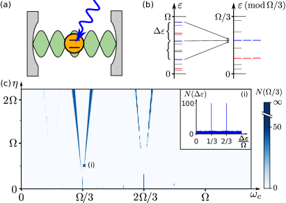
Figure 1: (a) We study a 2-level system (orange), coupled to a single cavity mode (green) while driven periodically with frequency $\Omega$ (blue). (b) Quasienergy locking: while the quasienergies of the system (gray, red, and blue lines) are effectively uniformly distributed between $0$ and $\Omega$, in certain finite parameter regimes the spacings between certain subsets of levels (red and blue) are exponentially close to $\Omega/q$ for some integer $q$ (here we illustrate this clustering for $q=3$). (c) Number of period-3 quasienergy-locked levels in the model, obtained from numerical exact evolution and diagonalization of the system’s Floquet operator, as function of cavity frequency $\omega_{\rm c}$ and qubit-cavity coupling $\eta$ (see Sec. II for model details, Sec. V for details of the simulation, and Appendix B for similar plots for other frequency locking ratios). The inset shows a histogram of quasienergy level spacings in the frequency-locked regime (parameters indicated by the cross in main panel).

In this work, we consider another class of such driving-induced phenomena: quantum frequency locking [51, 38, 42, 52, 30, 53, 54, 55]. Quantum frequency locking arises when a quantum system with an intrinsic characteristic frequency $\omega_{\rm c}$ is driven at a frequency $\Omega=2\pi/T$ close to (but not necessarily equal to) a rational multiple $q/r$ of the intrinsic frequency $\omega_{\rm c}$. In this case, the system can respond by robust oscillations with period locked exactly to an integer multiple of the driving period, $qT$.

Here we propose a new and accessible realization of quantum frequency locking. Namely, we consider a periodically-driven qubit coupled to a quantized electromagnetic cavity (Fig. 1a). When the qubit is driven close to resonance with a rational multiple of the cavity’s resonance frequency, the cavity mode oscillates with frequency locked to $r\Omega/q$. This phenomenon has a wide range of interesting implications and uses, which we explore in this paper: in particular, it implies the formation of characteristic subsets of quasienergy levels which are separated by $\Omega/q$, up to exponentially small corrections (see sketch in Fig. 1b) [51, 42]; we term this related phenomenon “quasienergy locking.” Quantum frequency locking is, moreover, a robust effect, which does not require fine-tuning [56]. It persists both for weak and strong qubit-cavity coupling, and for finite ranges of the driving frequency (see Fig. 1c).

Quantum frequency locking has previously been considered in various platforms and settings, including ultracold atoms interacting with a vibrating mirror [38, 55], spin chains or clock-models [47, 57, 54], parametrically driven chains of electromagnetic cavities [58], and nonlinear oscillators [51, 59, 42]. Our proposal provides a new and complimentary realization that can capitalize on recent advances in control of few-level quantum systems in Rydberg atoms, quantum dots, and superconducting qubits interacting with microwave cavities [60, 61, 62]. In this way our results provide a direct path for realizing quantum frequency locking on readily-available experimental platforms. In addition to being of fundamental interest, the robust coherent oscillations of the cavity mode can moreover be used as a frequency converter to generate a coherent signal at a frequency different from the drive (by a factor $r/q$).

Quantum frequency locking has a well-established classical counterpart, known as Arnold Tongues [63, 64, 32, 65, 66]. Quantum mechanics, however, introduces several new aspects to this effect: the wave-packets of a system do not spread in phase space when observed stroboscopically [67, 58]. Moreover, as explained above, the robust period-multiplied oscillations implies a nontrivial ordering of the quasienergy spectrum in the system (see Fig. 1b). The Wigner functions of the corresponding Floquet eigenstates exhibit a remarkably rich structure (see Fig. 2cd below).

The nontrivial organization of the quasienergy spectrum mentioned above is a signature of the breakdown of discrete time-translation symmetry [51, 38, 68, 42]. Thus frequency-locked quantum systems also present examples of “Floquet time-crystals” [14, 15], and demonstrate how time-translation symmetry breaking (in a broader sense than defined in Ref. 15) may be realized in few-body quantum systems [see also Refs. 38, 42]; see Sec. IV for further discussion.

In what follows we introduce the qubit-cavity model we study in Sec. II. In Sec. III, we perform an approximate semiclassical analysis of the model to describe how quantum frequency locking emerges, and identify the conditions under which it occurs. We discuss the implications of quantum frequency locking for the quasienergy spectrum of the system in IV, before confirming our approach numerically in Sec. V. Here we also discuss how quantum frequency locking may be utilized for frequency conversion (Sec. V.3). We conclude with a discussion in Sec. VI. Technical details of our analysis are provided in the Appendices.

II model

The system we consider consists of a two-level system, such as a qubit, quantum dot, or a spin-1/2 magnetic moment, coupled linearly to a quantized electromagnetic cavity mode, and to a periodic drive (see Fig. 1a). Without loss of generality, we refer to the two-level system simply as a spin below.

The Hamiltonian of the system is given by

$$\hat{H}(t)=\hat{H}_{\rm c}+\hat{H}_{\rm s}(t).$$ (1)

Here $\hat{H}_{\rm c}$ and $\hat{H}_{\rm s}(t)$ denote the Hamiltonian of the cavity and spin, respectively, defined such that $\hat{H}_{\rm s}(t)$ includes the spin-cavity coupling; this term [and hence also $\hat{H}(t)$] depends on time $t$. The cavity Hamiltonian is simply given by $\hat{H}_{\rm c}=\omega_{\rm c}\hat{b}^{\dagger}\hat{b}$, where $\omega_{\rm c}$ and $\hat{b}$ denote the frequency and bosonic annihilation operator of the cavity mode, respectively (here and below, we work in units where $\hbar=1$). The Hamiltonian of the spin, $\hat{H}_{\rm s}(t)$, consists of three parts: a static (Zeeman) part, $\hat{H}_{0}$, a term coupling the spin to a time-dependent driving field, $\hat{V}_{\rm dr}(t)$, and a term coupling the spin to the cavity field, $\hat{H}_{\rm sc}$:

$$\hat{H}_{\rm s}(t)=\hat{H}_{0}+\hat{V}_{\rm dr}(t)+\hat{H}_{\rm sc}.$$ (2)

The drive encoded in $\hat{V}_{\rm dr}(t)$ has $T$-periodic time-dependence (angular frequency $\Omega\equiv{2\pi}/{T}$): $\hat{V}_{\rm dr}(t)=\hat{V}_{\rm dr}(t+T)$.

We do not expect frequency-locking to depend on the specific details of $\hat{H}_{0}$, $\hat{V}_{\rm dr}(t)$ and $\hat{H}_{\rm sc}$. For concreteness, however, we use the forms:

$$\hat{H}_{0} = \eta\hat{\sigma}_{x}B_{0},$$ (3)

$$\hat{V}_{\rm dr}(t) = \eta A_{d}[\sin(\Omega t)\hat{\sigma}_{x}+\cos(\Omega t)\hat{\sigma}_{z}],$$ (4)

$$\hat{H}_{\rm sc} = \eta(\hat{b}\hat{\sigma}^{+}+\hat{b}^{\dagger}\hat{\sigma}^{-}).$$ (5)

Here $\eta$ parametrizes the spin’s coupling to the external (Zeeman and driving) fields and to the cavity field, $\hat{\sigma}_{x},\hat{\sigma}_{y},\hat{\sigma}_{z}$ denote the Pauli matrices acting on the spin, with $\hat{\sigma}^{\pm}\equiv\frac{1}{2}(\hat{\sigma}_{x}\pm i\hat{\sigma}_{y})$, and $B_{0}$ and $A_{d}$ are dimensionless numbers denoting the effective Zeeman field strength and driving amplitude, respectively. This model was shown to support topological frequency conversion in Refs. 16, 17, 18.

The cavity mode is described by a harmonic oscillator, and can thus conveniently be represented using the dimensionless position and momentum operators [69] $\hat{x}\equiv\frac{1}{2}(\hat{b}+\hat{b}^{\dagger})$ and $\hat{p}\equiv\frac{1}{2i}(\hat{b}-\hat{b}^{\dagger})$. In terms of these operators, the Hamiltonian of the full system is given by

$$\hat{H}(t)=\frac{\omega_{c}}{2}(\hat{x}^{2}+\hat{p}^{2})+\eta{\bf b}(\hat{x},\hat{p},t)\cdot{\bf\hat{S}},$$ (6)

where ${\bf\hat{S}}=(\hat{\sigma}_{x},\hat{\sigma}_{y},\hat{\sigma}_{z})$ denotes the effective spin operator describing the qubit, while

$${\bf b}(x,p,t)=(B_{0}-A_{d}\sin\Omega t-x,p,A_{d}\cos\Omega t)$$ (7)

can be seen as the effective Zeeman field acting on the spin, as a function of the cavity mode’s position and momentum, and time.

As mentioned in the introduction, the model above can be realized in various ways. Most appealing perhaps are realizations using superconducting qubits [70, 71, 62] and nitrogen-vacancy (NV) centers [72, 73], as well as atoms in optical cavities (see, e.g., Refs. 74, 75). We expect that our following discussion generalizes to cavities with multiple modes [17].

III Semiclassical picture of Frequency locking

When the driving field of the in model of Sec. II has an off-resonant frequency, $\Omega$, close to a rational multiple $q/r$ of the cavity eigenfrequency $\omega_{\rm c}$ (where $q$ and $r$ are integers), there exists finite regions of phase space where the cavity mode responds to the drive with coherent oscillations whose frequency is locked exactly to $r\Omega/q$. We refer to this phenomenon as quantum frequency locking. In this section, we demonstrate from heuristic semiclassical arguments how quantum frequency locking arises in the model. We confirm our approach using numerical simulations in Sec. V.

Our first step towards deriving frequency locking is to transform the cavity mode’s degrees of freedom, $(\hat{x},\hat{p})$, to a frame rotating with frequency $\tilde{\Omega}\equiv r\Omega/q$ (as in previous studies of quantum frequency locking; see, e.g., Refs. [59, 42]). In this rotating frame, the cavity mode becomes much slower than the driving period and the spin’s dynamics. In Sec. III.1, we identify conditions under which this separation of time scales allows us to effectively integrate out the spin and the driving field. This results in a time-independent semiclassical effective Hamiltonian that governs the evolution of the cavity mode in the rotating frame:

$$\mathcal{H}_{\rm eff}(x,p)=\frac{\delta\omega}{2}\left(x^{2}+p^{2}\right)+\varepsilon(x,p),$$ (8)

where $x$ and $p$ denote the semiclassical position and momentum variables of the cavity mode (in the rotating frame), and $\delta\omega\equiv\omega_{c}-\tilde{\Omega}$ is the cavity detuning from $\tilde{\Omega}$. The potential $\varepsilon(x,p)$ in Eq. (8) results from integrating out the spin and the driving field, and plays a central role in our analysis. We identify two distinct parameter regimes where the above separation of timescale occurs, namely, the large-$\eta$ adiabatic regime, and the small-$\eta$ Floquet regime (see Sec. III.1 for discussion of these regimes). Both regimes support quantum frequency locking, but result in two distinct expressions for the potential $\varepsilon(x,p)$.

Frequency locking can naturally be understood by inspecting the effective Hamiltonian $\mathcal{H}_{\rm eff}(x,p)$: in Fig. 2ab we plot $\mathcal{H}_{\rm eff}(x,p)$ for the two regimes where quantum frequency locking occurs with period $3$. In both cases $\mathcal{H}_{\rm eff}(x,p)$ has local extrema at nonzero values of $x$ and $p$. When the cavity mode is initialized at one of these extrema, its phase space location in the rotating frame remains stationary. As a result, in the original “lab” frame, the cavity mode will oscillate with frequency $\Omega/3$.

The picture above also explains the robustness of frequency locking. Even if the cavity is initialized near (but not precisely at) the extremum of $\mathcal{H}_{\rm eff}$, its location in the rotating frame will remain confined near the extremum at all times. Thus, frequency locking can be achieved with only moderate requirements for control over initial conditions; for instance, in Fig. 2, it will occur with significant probability as long as the displacement amplitude of the cavity mode, $\sqrt{x^{2}+p^{2}}$, is less than $30$ in the dimensionless units we have adopted [see text above Eq. (6)]. The corresponding motion in the lab frame must remain close to this point each time three driving periods have passed. As a result, the frequency spectrum of the cavity mode’s motion features a sharp, well-defined peak at $\Omega/3$. The extrema moreover cannot be removed by weak perturbations, implying that frequency locking persists in finite parameter ranges.

In Appendix A we present a different, complementary perspective on quantum frequency locking, based on the dynamics in the combined Fock space of the oscillator and driving field. The approach presented there can in principle be used to study quantum frequency locking for any driven finite-dimensional quantum system coupled to a quantized cavity mode, in the limit of small nonlinearity and detuning.

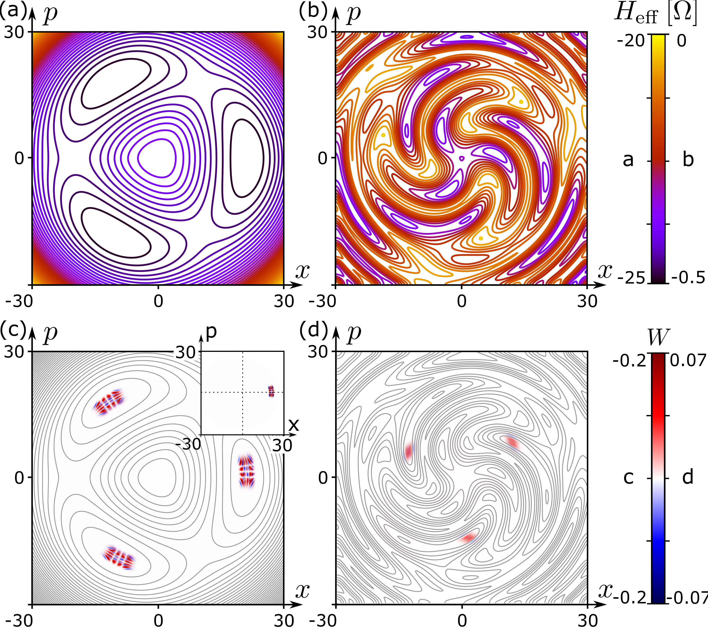
Figure 2: (a) and (b): Constant (quasi)energy contours of the effective Hamiltonian for the cavity mode in the frame where phase space rotates with frequency $\Omega/3$, $\mathcal{H}_{\rm eff}(x,p)$, [see Eq. (8)], Panels (a) and (b) depict two parameter sets where period-$3$ quantum frequency locking occurs, within the adiabatic and Floquet regimes, respectively; see Sec. III.1 for parameters. (c) and (d): Wigner functions of quasienergy-locked Floquet eigenstates, using the same parameters as in panels (a) and (b), respectively. The contours of the corresponding effective Hamiltonians from panels (a) and (b) shown as grey lines. Inset, panel (c): Wigner function for an equal-weight linear combination of the $3$ related Floquet eigenstates of which one is depicted in (c) (see Sec. IV).

III.1 Effective cavity mode Hamiltonian

We now obtain the effective Hamiltonian in Eq. (8). To this end, we consider the dynamics of the system in the rotating frame that was described above. The Hamiltonian of the system in this rotating frame is given by $\tilde{H}(t)=\hat{U}^{\dagger}_{0}(t)\big{[}\hat{H}(t)-\tilde{\Omega}\hat{b}^{\dagger}\hat{b}\big{]}\hat{U}_{0}(t),$ where the unitary operator $\hat{U}_{0}(t)\equiv e^{-i\tilde{\Omega}\hat{b}^{\dagger}\hat{b}t}$ generates the transformation to the rotating frame: the Schrödinger equation in the lab frame is solved by $|\psi(t)\rangle=\hat{U}_{0}(t)|\tilde{\psi}(t)\rangle$, where $\partial_{t}|\tilde{\psi}(t)\rangle=-i\tilde{H}(t)|\tilde{\psi}(t)\rangle$. Noting that $\hat{U}_{0}(t)$ only acts nontrivially on $\hat{H}_{\rm sc}$, we find

$$\tilde{H}(t)=\frac{\delta\omega}{2}(\hat{x}^{2}+\hat{p}^{2})+\eta{\bf h}(\hat{x},\hat{p},t)\cdot{\bf\hat{S}},$$ (9)

where ${\bf h}$ is obtained from ${\bf b}$ in Eqs. (6) and (7) after rotating the oscillator phase space by $\tilde{\Omega}t$: ${\bf h}(x,p,t)={\bf b}\big{(}x\cos\tilde{\Omega}t+p\sin\tilde{\Omega}t,p\cos\tilde{\Omega}t-x\sin\tilde{\Omega}t,t\big{)}$. Note that the Hamiltonian $\tilde{H}(t)$ in Eq. (9) describes a periodically driven system with extended period $\tilde{T}=qT$, through the explicit time-dependence of ${\bf h}(x,p,t)$ above (recall that $\tilde{\Omega}=r\Omega/q$).

To derive the effective semiclassical Hamiltonian for the cavity mode, $\mathcal{H}_{\rm eff}(x,p)$, we consider the equations of motion generated by $\tilde{H}(t)$ for the Heisenberg picture operators $\hat{x}(t)$, $\hat{p}(t)$, and ${\bf\hat{S}}(t)$:

$$\partial_{t}\hat{x}(t) =\delta\omega\,\hat{p}(t)+\eta{\bf v}_{p}(t)\cdot{\bf\hat{S}},$$ (10)

$$\partial_{t}\hat{p}(t) =-\delta\omega\,\hat{x}(t)-\eta{\bf v}_{x}(t)\cdot{\bf\hat{S}},$$ (11)

$$\partial_{t}{{\bf\hat{S}}}(t) =\eta{\bf h}[\hat{x}(t),\hat{p}(t),t]\times{\bf\hat{S}}.$$ (12)

where ${\bf v}_{x}(t)$ and ${\bf v}_{p}(t)$ are vectors with unit norm: ${\bf v}_{x}(t)\equiv(-\cos\tilde{\Omega}t,\sin\tilde{\Omega}t,0)$, ${\bf v}_{p}(t)\equiv(\sin{\tilde{\Omega}}t,\cos{\tilde{\Omega}}t,0)$. We apply a semiclassical approximation to the equations of motion above, by assuming that the cavity mode’s location in phase space is relatively well-defined at all times: in Eq. (12), we approximate ${\bf h}(\hat{x}(t),\hat{p}(t),t)\approx{\bf h}(x(t),p(t),t)$, where $x(t)\equiv\langle\hat{x}(t)\rangle$, and $p(t)\equiv\langle\hat{p}(t)\rangle$ denote the expectation values of the position and momentum operators. We expect this approximation to be justified when the characteristic scales in phase space of variations in ${\bf h}(x,p,t)$ are large compared to the scale of quantum fluctuations $\Delta x,\Delta p\sim 1$.

The approximation above reduces Eq. (12) to a Bloch-equation with a time-dependent field ${\bf h}(x(t),p(t),t)$. By moreover taking the expectation values on both sides of Eqs. (10)-(12), we then obtain three coupled equations of motion for the (semi)classical variables $x(t),p(t),$ and ${\bf S}(t)\equiv\langle{\bf S}(t)\rangle$: namely Eqs. (10)-(12) with the operators $\hat{x}(t)$, $\hat{p}(t)$, and ${\bf\hat{S}}(t)$ replaced by their expectation values $x(t)$, $p(t)$, and ${\bf S}(t)$. These equations of motion are generated by the time-dependent classical Hamiltonian $\tilde{\mathcal{H}}(t)$, given by

$$\tilde{\mathcal{H}}(t)=\frac{\delta\omega}{2}(x^{2}+p^{2})+\eta{\bf h}(x,p,t)\cdot{\bf S}.$$ (13)

Note that the dynamics of the cavity mode, $(x(t),p(t))$, has characteristic frequencies $\delta\omega,\eta$, which can be much smaller than $\tilde{\Omega}$ (which is on the same order as the resonance frequency of the oscillator) and the characteristic frequencies of the spin’s dynamics. Below, we identify two parameter regimes where this separation of timescales allows us to effectively eliminate the spin, ${\bf S}(t)$, and obtain the static effective Hamiltonian for the cavity mode in Eq. (8).

III.1.1 Adiabatic regime

The simplest “adiabatic” regime occurs for large $\eta$. In this regime the direction of the instantaneous Zeeman field, ${\bf h}(x(t),p(t),t)$, changes adiabatically with respect to the (fast) Larmor precession of the spin, which has frequency $\sim\eta|{\bf h}(x,p,t)|$ [see Eq. (13)]. In this case, the equations of motion [Eq. (12) with $\hat{x},\hat{p}$, and ${\bf\hat{S}}$ substituted by their expectation values $x$ and $p$] has the two distinct solutions: ${\bf S}(t)\approx\pm{\bf h}(x,p,t)/|{\bf h}(x,p,t)|$ [76]. With these solutions for ${\bf S}$, Eq. (13) becomes

$$\tilde{\mathcal{H}}^{\pm}_{\rm cav}(x,p,t)=\frac{\delta\omega}{2}(x^{2}+p^{2})\pm\eta|{\bf h}(x,p,t)|.$$ (14)

Similarly to quantum systems, the stroboscopic time-evolution generated by $\tilde{\mathcal{H}}^{\pm}_{\rm cav}(x,p,t)$ (i.e., time-evolution at integer multiples of $\tilde{T}$) is equivalent to that generated by some time-independent effective classical Hamiltonian [77]. When the cavity mode in the rotating frame oscillates slowly compared to $\tilde{\Omega}$ (see below for more detailed conditions), this effective Hamiltonian is well-approximated by the time-average of $\tilde{\mathcal{H}}_{\rm cav}^{\pm}(x,p,t)$; i.e., by $\mathcal{H}_{\rm eff}(x,p)$ in Eq. (8), with

$$\varepsilon(x,p)=\pm\frac{\eta}{{\tilde{T}}}\int_{0}^{{\tilde{T}}}\!\!\!{\rm d}t\,|{\bf h}(x,p,t)|,$$ (15)

where the sign ($\pm$) depends on the initial alignment of the spin [76]. Eq. (15) can be obtained using a Magnus expansion of the evolution operator generated by the system’s Liouvillian (see Ref. [77] for details).

The considerations above show that $\mathcal{H}_{\rm eff}(x,p)$ in Eqs. (8) and (15) describes the system when the Larmor precession frequency of the spin, $\eta|{\bf h}(x,p,t)|$ is much larger than the driving frequency, which in turn should be much larger than the characteristic frequency of the cavity mode in the rotating frame. The latter is given by the renormalized frequency detuning $\delta\omega^{\prime}(x,p)$, given by the radial gradient of $\mathcal{H}_{\rm eff}(x,p)$, divided by the amplitude of the cavity mode, $A_{\rm cav}=\sqrt{x^{2}+p^{2}}$. Hence the adiabatic regime arises when $\delta\omega^{\prime}(x,p)\ll\Omega\ll\eta|{\bf h}(x,p,t)|$ (here we used that $\Omega$ and $\tilde{\Omega}$ have the same order of magnitude). This condition is satisfied in the vicinity of the extrema of $\mathcal{H}_{\rm eff}(x,p)$, as long as these occur in regions of phase space where $\eta|{\bf h}(x,p,t)|\gg\Omega$. As an illustration, in Fig. 2a, we plot the constant (quasi)energy contours of $\mathcal{H}_{\rm eff}(x,p)$ in the adiabatic regime, obtained from direct numerical evaluation of Eqs. (8) and (15). We use the parameters $A_{d}=15$, $B_{0}=7$, $\omega_{c}=0.34\Omega$ and $\eta=0.56\Omega$. These parameters are indicated by the cross in Fig. 1c, and fall within the adiabatic regime. We expect $\mathcal{H}_{\rm eff}(x,p)$ to describe the system accurately near the three minima located at radius $A_{\rm cav}\approx 24$, where its gradient (and hence $\delta\omega^{\prime}$) vanishes. In Sec. V (see also Fig. 1c), we confirm that these local minima indeed lead to quantum frequency locking at these parameters, as explained above.

III.1.2 Floquet regime

The Floquet parameter regime for frequency locking occurs not when the instantaneous Hamiltonian changes adiabatically, but rather when the effective Floquet Hamiltonian of the spin (with $x$ and $p$ held fixed) changes adiabatically.

To obtain the effective Hamiltonian $\mathcal{H}_{\rm eff}(x,p)$ in the Floquet regime, we consider the dynamics resulting from Eq. (12) with $x$ and $p$ held fixed. In this case, the time-periodicity of ${\bf h}(x,p,t)$ implies that all solutions ${\bf S}(t)$ to Eq. (12) satisfy ${\bf S}([n+1]\tilde{T})=R_{0}(x,p){\bf S}(n\tilde{T})$, for some fixed three-dimensional orthogonal matrix $R_{0}(x,p)$ with unit determinant. Like any orthogonal matrix with unit determinant, $R_{0}(x,p)$ can be expressed as a rotation about some axis ${\bf a}(x,p)$ by some angle $\theta(x,p)$ between $0$ and $\pi$ (note that the required interval for $\theta$ fixes the direction of ${\bf a}$). As a result, for fixed $x$ and $p$, there exists a time-periodic solution to the Bloch equation in Eq. (12) (up to a constant scale factor), ${\bf S}(t)={\bf n}_{0}(x,p,t)$, in which ${\bf n}_{0}(x,p,0)={\bf a}(x,p)$ is parallel to the net rotation axis, and ${\bf n}_{0}(x,p,t)$ evolves according to Eq. (12). Thus, for fixed $x$ and $p$, we identify $\mathcal{H}_{\rm eff}^{{\rm spin}}(x,p)=\theta(x,p){\bf a}(x,p)\cdot{\bf S}$ as the effective Hamiltonian of the spin (see Appendix C for further details).

When $x$ and $p$ are not fixed, but the evolution of effective precession axis ${\bf a}(x,p)$ (due to the motion of $x$ and $p$) evolves slowly relative to the energy gap of $H_{\rm eff}^{{\rm spin}}$, $\delta\varepsilon(x,p)\equiv\min(\theta(x,p),2\pi-2\theta(x,p))/\tilde{T}$ (see Appendix C), the stroboscopic motion of the spin closely follows stroboscopic motion resulting from the adiabatically changing Hamiltonian $H_{\rm eff}^{{\rm spin}}(x(t),p(t))$ [78]. As a result, if initially aligned or anti-aligned with ${\bf a}(x(0),p(0))$, the spin’s evolution at later (stroboscopic) times will satisfy ${\bf S}(n\tilde{T})\approx\pm{\bf a}(x(n\tilde{T}),p(n\tilde{T}))$, where the sign depends on the initial alignment. In Appendix C, we substitute this solution into Eq. (13) and take the time-average, making use of our assumption that the cavity mode is effectively stationary within the driving period $\tilde{T}$ [77]. Doing this, we find that the cavity mode evolves according to the effective Hamiltonian in Eq. (8), with

$$\varepsilon(x,p)=\pm\theta(x,p)/2\tilde{T}.$$ (16)

Here the sign depends on the initial alignment of the spin with ${\bf a}(x,p)$ [76]. The angle $\theta(x,p)$ can be straightforwardly calculated for the system by exact time-evolution of the Bloch equation for the spin in Eq. (12).

The Floquet regime arises when the dynamics of the cavity mode occur on a much longer time-scale than the driving period $\tilde{T}$, and when the change of the effective axis of rotation, ${\bf a}(x,p)$ (due to the motion of $x$ and $p$) is slow compared to the effective Larmor frequency $\theta(x,p)/\tilde{T}$. In Appendix C, we show that these conditions are satisfied when $\eta\ll\theta(x,p)/\tilde{T}$ and $\delta\omega\ll\tilde{\Omega}/A_{\rm cav}$, where $A_{\rm cav}=\sqrt{x^{2}+p^{2}}$ denotes the amplitude of the cavity field. Note that, since $\tilde{T}>T$, and $\theta(x,p)\leq\pi$, the Floquet regime requires $\eta\ll\Omega$. Thus the Floquet regime arises in the limit of small spin-cavity coupling, $\eta$, and detuning, $\delta\omega$ (since our semiclassical approximation requires $A_{\rm cav}\gg 1$ for quantum fluctuations not to play a role).

As an illustration, In Fig. 2b, we plot the contours of $\mathcal{H}_{\rm eff}(x,p)$ for antialigned spin (i.e., with ${\bf S}=-{\bf a}$) using the parameters $A_{d}=15,B_{0}=7,\omega_{c}=\Omega/3$ and $\eta=0.048\Omega$. Since $\delta\omega=0$, the conditions for Floquet locking outlined above imply that $\mathcal{H}_{\rm eff}$ accurately describes the dynamics of the cavity mode whenever $H_{\rm eff}(x,p)\gg\eta$.

IV Quasienergy locking and symmetry breaking

In Sec. III, we identified the conditions for quantum frequency locking: namely, it arises for parameters in the adiabatic or Floquet regimes where the effective Hamiltonian $\mathcal{H}_{\rm eff}(x,p)$ [Eq. (8)] has extrema at nonzero amplitude in phase space. While our treatment in Sec. III in principle also applies to fully classical systems (indeed, our results were derived using semiclassical arguments), in this section we demonstrate some novel aspects of the quantum mechanical version of the phenomenon. In particular, we show that period-$q$ quantum systems feature characteristic multiplets of quasienergy levels that differ by rational fractions of the drive frequency, $\Omega/q$, up to exponentially suppressed corrections [see Eq. (17) below]. We term this phenomenon “quasienergy locking”. It was also identified in earlier work [51, 38, 15, 42], and can be seen as the defining feature of quantum frequency locking.

Quasienergy locking can be seen as a breakdown of the discrete time translation symmetry which is inherently present in the driven system [38, 15, 42]: as we show below, linear combinations of quasienergy-locked Floquet eigenstates define a family of nearly stationary states of the system’s evolution that break the discrete time translation symmetry of the drive (up to exponentially long times).

In the remainder of this section we review the defining features of quasienergy locking (Sec. IV.1), and subsequently show how it arises the qubit-cavity model (Sec. IV.2). We finally discuss how quasienergy locking can be understood as a breakdown of discrete time translation symmetry (Sec. IV.3). To highlight physical aspects of the phenomenon, we provide our arguments on a heuristic level, while a more rigorous (but technical) treatment is given in Appendix. D.

IV.1 Quasienergy locking

Quasienergy locking is a phenomenon that arises in the quasienergy spectrum of periodically driven quantum systems [51, 38, 15, 42]. In such systems the quasienergies $\{\varepsilon_{n}\}$ define the eigenvalues of the system’s time-evolution operator over one period (known as the Floquet operator), $\hat{U}(T)|\psi_{n}\rangle=e^{-i\varepsilon_{n}T}|\psi_{n}\rangle$, where $\hat{U}(t)\equiv Te^{-i\int_{0}^{t}dt^{\prime}\hat{H}(t^{\prime})}$ denotes the system’s time-evolution operator and $\mathcal{T}$ denotes the time-ordering operation. The corresponding eigenstates $\{|\psi_{n}\rangle\}$, termed Floquet eigenstates, hence form a complete basis of states that are mapped to themselves after each driving period $T$, up to a unitary phase $e^{-i\varepsilon_{n}T}$. Quasienergy thus plays a role analogous to energy for the evolution of periodically driven quantum systems: the evolution at integer multiples of the driving period, $k$, can be resolved as $|\psi(kT)\rangle=\sum_{n}c_{n}e^{-i\varepsilon_{n}kT}|\psi_{n}\rangle,$ where the coefficients $\{c_{n}\}$ are determined from the initial conditions [79]. However, note that each $\varepsilon_{n}$ is only defined modulo $\Omega$.

The quasienergies of a generic periodically driven quantum system are naturally distributed uniformly between $0$ and $\Omega$. However, when period-$q$ quantum frequency locking arises, the spectrum features characteristic multiplets of quasienergy levels $\varepsilon_{1},\ldots\varepsilon_{q}$ that differ by $\Omega/q$, up to exponentially suppressed corrections:

$$\varepsilon_{\ell}=\varepsilon+\ell\Omega/q+\mathcal{O}(\delta\varepsilon),$$ (17)

where $\varepsilon$ generally differs from multiplet to multiplet. Here $\delta\varepsilon$ is a quasienergy scale that can be many times smaller than the average quasienergy level spacing in the system, such that the feature above would not occur by coincidence (see, e.g., the inset in Fig. 1c and Sec. V). For the driven qubit-cavity system we consider in this work, we show below that $\delta\varepsilon\sim e^{-d/\xi}$, where $d$ denotes the separation in phase space between the extrema of the effective Hamiltonian $\mathcal{H}_{\rm eff}(x,p)$, while $\xi\sim 1$ denotes the scale of quantum fluctuations. We term the formation of these multiplets “quasienergy locking”.

The Floquet eigenstates associated with each multiplet of locked quasienergy levels, $|\psi_{1}\rangle,\ldots|\psi_{q}\rangle$, have interesting features of their own. Specifically, they take the form

$$|\psi_{\ell}\rangle=\frac{1}{\sqrt{q}}\sum_{k=1}^{q}e^{-2\pi i\ell k/q}|\chi_{k}\rangle,$$ (18)

where, for the model we consider, each state $|\chi_{k}\rangle$ has support only near a particular extremum of $\mathcal{H}_{\rm eff}(x,p)$ in phase space (see Appendix D and Sec. IV.2 below). Note from Eq. (18) that, for each $k$, $|\chi_{k}\rangle\equiv\frac{1}{\sqrt{q}}\sum_{k}e^{2\pi i\ell k/q}|\psi_{k}\rangle$. One can thus verify that the states $|\chi_{1}\rangle\ldots|\chi_{k}\rangle$ are orthogonal, and mapped to each other under evolution by one driving period $T$, up to a phase and an exponentially suppressed correction:

$$\hat{U}(T)|\chi_{k}\rangle=e^{-i\varepsilon T}|\chi_{k+1}\rangle+\mathcal{O}(\delta\varepsilon T),$$ (19)

with $|\chi_{q+1}\rangle\equiv|\chi_{q}\rangle$ [80].

IV.2 Derivation of quasienergy locking for the driven qubit-cavity system

Having reviewed the defining features of quasienergy locking, we now show how it emerges in the driven qubit-cavity system that we consider in this work. We provide our arguments on a heuristic basis, by analyzing the dynamics of the system in the rotating frame introduced in Sec. III.1. For simplicity we consider the limit where the evolution of the system in this frame is fully captured by the effective semiclassical Hamiltonian from Sec. III, $\mathcal{H}_{\rm eff}(x,p)$ (see Sec. III.1 for specific conditions). In Appendix C we provide a more rigorous line of arguments that holds in the Floquet and adiabatic limits whenever $\mathcal{H}_{\rm eff}(x,p)$ features extrema with surrounding “potential wells” that are much larger than the scale of quantum fluctuations, $\xi\sim 1$ (see below for definition of potential wells).

To derive quasienergy locking we investigate the properties of the driven qubit-cavity system’s Floquet eigenstates and quasienergies, $\{|\psi_{n}\rangle\}$ and $\{\varepsilon_{n}\}$. As a first step, we note that the former are identical to the Floquet eigenstates in the rotating frame (see Sec. III.1), $\{|\tilde{\psi}_{n}\rangle\}$, while each quasienergy $\varepsilon_{n}$ is identical to the corresponding quasienergy in the rotating frame, $\tilde{\varepsilon}_{n}$, modulo $\tilde{\Omega}\equiv\Omega/q$ [81]. To obtain $\{|\tilde{\psi}_{n}\rangle\}$ and $\{\tilde{\varepsilon}_{n}\}$, we we recall our assumption that $\mathcal{H}_{\rm eff}(x,p)$ fully captures the system’s dynamics in the rotating frame. Hence we expect the stroboscopic evolution of the quantized cavity mode (in the rotating frame) to be generated by the effective quantum Hamiltonian $\mathcal{H}_{\rm eff}(\hat{x},\hat{p})$. We moreover expect the spin to be locked to the effective axis of precession as a function of $x$ and $p$, as explained in Sec. III. For simplicity, we therefore neglect the spin in the following. Through the above correspondence between the rotating and lab frames, in the idealized limit we consider here, the Floquet eigenstates of the system in the lab frame are thus given by the eigenstates of $\mathcal{H}_{\rm eff}(\hat{x},\hat{p})$, while the quasienergies are given by the corresponding eigenvalues, up to integer multiples of $\tilde{\Omega}$.

To obtain the eigenstates and eigenvalues of $\mathcal{H}_{\rm eff}(\hat{x},\hat{p})$, we consider the structure of $\mathcal{H}_{\rm eff}(\hat{x},\hat{p})$ in the frequency-locked regime. We recall that frequency locking arises when $\mathcal{H}_{\rm eff}(x,p)$ has extrema at nonzero displacement amplitude. These extrema are surrounded by classical trajectories [i.e., contours of $\mathcal{H}_{\rm eff}(x,p)$] which encircle and remain close to their respective fixed points at all times. We refer to each such extremum, along with its surrounding neighborhood that contains these encircling trajectories (out to the separatrices beyond which the trajectories encircle other fixed points) as a potential well. Note that $\mathcal{H}_{\rm eff}(x,p)$ has a built-in symmetry of discrete rotation by $2\pi/q$ in phase space, as is evident in the numerical examples plotted in Fig. 2ab, where $q=3$ (see also Appendix D). This symmetry, which is generated by $\hat{U}_{0}(T)$, guarantees that each potential well of $\mathcal{H}_{\rm eff}(x,p)$ forms part of a ring of $q$ wells which are mapped to each other through rotations by $2\pi/q$ in phase space. We refer to these wells as wells $1\ldots q$ in the following, such that well $k$ is mapped to well $k+1\,({\rm mod}\ q)$ a through phase space rotation by $2\pi/q$.

We expect $\mathcal{H}_{\rm eff}(\hat{x},\hat{p})$ to support approximate eigenstates that are confined within the potential wells of $\mathcal{H}_{\rm eff}(x,p)$, whose wave functions decay with the distance from the well, $r$, as $\mathcal{O}(e^{-r/\xi})$. For $k=1,\ldots q$, we let $|\phi_{k}\rangle$ denote such a “bound” eigenstate of $\mathcal{H}_{\rm eff}(\hat{x},\hat{p})$ when restricting phase space to well $k$, such that $|\phi_{k}\rangle$ and $|\phi_{k+1}\rangle$ are related through phase space rotation by $2\pi/q$; i.e., we restrict phase space to a region located within a distance $r_{0}$ from well $k$, for some $0<r_{0}<d/2$, where $d$ denotes the distance in phase space between adjacent wells. We let $\varepsilon$ denote the corresponding eigenvalue of $H_{\rm eff}(\hat{x},\hat{p})$; this takes the same value for all $k$ due to the discrete rotation symmetry. Below we find that the bound states $\{|\phi_{k}\rangle\}$ are identical to the states $\{|\chi_{k}\rangle\}$ whose linear combinations give a quasienergy-locked multiplet of Floquet eigenstates as in Eq. (18). Note, however, that this identification is only exact in the idealized limit we consider here, where ${\mathcal{H}}_{\rm eff}(\hat{x},\hat{p})$ fully captures the stroboscopic evolution in the rotating frame. Beyond this limit, $\{|\chi_{k}\rangle\}$ deviate from $\{|\phi_{k}\rangle\}$ by nonzero, but small, corrections due to, e.g., nonadiabatic corrections and quantum fluctuations. In Appendix D, we provide a more rigorous way to identify the states $|\chi_{n}\rangle$ that includes such corrections.

Due to the exponentially decaying wavefunction of $|\phi_{k}\rangle$ outside well $k$, when all of phase space is included, each $|\phi_{k}\rangle$ remains an approximate eigenstate of $\mathcal{H}_{\rm eff}(\hat{x},\hat{p})$, up to an exponentially small correction $\mathcal{H}_{\rm eff}(\hat{x},\hat{p})|\phi_{k}\rangle=\varepsilon|\phi_{k}\rangle+\mathcal{O}(e^{-r_{0}/\xi})$. To zeroth order in $\lambda=e^{-r_{0}/\xi}$ (i.e., in the classical limit $\xi\to 0$), each $|\phi_{k}\rangle$ is thus an exact eigenstate of $\mathcal{H}_{\rm eff}(\hat{x},\hat{p})$, with eigenvalue $\varepsilon$. In the limit of small but nonzero $\xi$, the corresponding eigenstates of $\mathcal{H}_{\rm eff}(\hat{x},\hat{p})$, $|\psi_{1}\rangle,\ldots|\psi_{q}\rangle$, can be obtained through zeroth-order degenerate perturbation theory, and thus can be expressed as linear combinations of the degenerate “unperturbed” states $|\phi_{k}\rangle$. To identify these linear combinations, we note that the discrete rotation symmetry $[\hat{U}_{0}(T),\mathcal{H}_{\rm eff}(\hat{x},\hat{p})]=0$ requires the eigenstates of $\mathcal{H}_{\rm eff}(\hat{x},\hat{p})$ to also be eigenstates of $\hat{U}_{0}(T)$. Since $\hat{U}_{0}(T)|\phi_{k}\rangle=|\phi_{k+1}\rangle$, $|\psi_{1}\rangle,\ldots|\psi_{q}\rangle$ are thus given by Eq. (18), with $|\chi_{n}\rangle=|\phi_{n}\rangle$. Using that $\langle\phi_{k}|\mathcal{H}_{\rm eff}(\hat{x},\hat{p})|\phi_{k^{\prime}}\rangle\lesssim e^{-d/\xi}$, we find that the corresponding eigenvalues of $\mathcal{H}_{\rm eff}(\hat{x},\hat{p})$, $\tilde{\varepsilon}_{1},\ldots\tilde{\varepsilon}_{q}$, are all given by $\varepsilon$, up to corrections of order $e^{-d/\xi}$. We conclude that for each ring of potential wells of $\mathcal{H}_{\rm eff}(x,p)$ (if such wells are present), the qubit-cavity system supports one or more families of Floquet eigenstates, whose form is given in Eq. (18), where, for each $k$, $|\chi_{k}\rangle$ has support only in well $k$ of the ring [82] . The corresponding quasienergies are given by the same value $\varepsilon$, up to integer multiples of $\Omega/q$, and corrections of order $e^{-d/\xi}$.

In Appendix D, we provide a more rigorous derivation of quasienergy locking, which holds beyond the idealized limit considered here. There we confirm that in the regime, the qubit-cavity system supports families of near-degenerate eigenstates of the form in Eq. (18), where $|\chi_{k}\rangle$ has support only in well $k$. However, $|\chi_{k}\rangle$ and $|\chi_{k+1}\rangle$ are not related by exact phase space rotation by $2\pi/q$, but rather through Eq. (19) [83]. It follows that the corresponding quasienergies take the form in Eq. (17). This was what we wanted to show in this subsection.

IV.3 Time translation symmetry breaking

Here we review how quasienergy locking can be seen as a realization of time-translation symmetry breaking [38, 15, 42]. To see this, note from Eq. (19) that the states $\{|\chi_{k}\rangle\}$ are taken onto themselves after evolution by the extended period $\tilde{T}=qT$, up to a phase, and an exponentially suppressed correction. Each $|\chi_{k}\rangle$ hence is a (nearly) stationary state of the system’s time-evolution that breaks the original discrete time-translation symmetry by $T$. In contrast to the exact Floquet eigenstates, $\{|\psi_{\ell}\rangle\}$, which are superpositions of states characterized by distinct values of the oscillator phase (i.e, “Schrödinger cat” states), each symmetry-breaking state $|\chi_{k}\rangle$ has a well-defined phase, and hence corresponds to a semiclassical “non-cat” state of the cavity mode. In the sense above, the driven qubit-cavity system can hence be seen as supporting steady states that break discrete time translation symmetry.

The symmetry-breaking states $\{|\chi_{k}\rangle\}$ remain stationary states of the system’s time-evolution up to the duration of confinement within the potential wells of $\mathcal{H}_{\rm eff}$, $\tau~{}\sim e^{{d/\xi}}$. In contrast, the “coherence time” of the symmetry-breaking steady states in many-body Floquet time crystals scales exponentially with the size of the system due to many-body nature of the states, and hence is infinite in the thermodynamic limit [14, 15]. For the qubit-cavity system we consider, although there is no thermodynamic limit, $\tau$ still scales exponentially with the system parameters, and thus can be very large compared to the other timescales of the system. In this sense, we can still regard time-translation symmetry to be broken in practice. Note that we consider a more general notion of time-translation symmetry breaking than defined in Ref [15]: namely, we only require some, but not all, steady states of the system to break the discrete time-translation symmetry of the system [38, 42].

V Numerical results

Here we support our discussion with numerical simulations. We simulate the qubit-cavity model in Sec. II by computing the complete Floquet operator of the system using direct time-evolution. We then obtain the quasienergy spectrum and Floquet eigenstates through exact diagonalization. In these simulations we truncate the Hilbert space of the cavity to the first $650$ photon-number eigenstates (resulting in Hilbert space dimension $1300$), and discretize the Hamiltonian’s continuous time-dependence within one period into $300$ evenly spaced intervals.

Throughout our simulations, we fix the dimensionless Zeeman field component to be $B_{0}=7$, and the driving amplitude $A_{d}=15$, while we vary the qubit-cavity coupling $\eta$ and the cavity resonance frequency $\omega_{\rm c}$ (see Sec. II).

V.1 Detection of quantum frequency locking

For each choice of the parameters $\eta$ and $\omega_{\rm c}$ we probed, we detected the presence of quantum frequency locking from the quasienergy spectrum of the system, $\{\varepsilon_{n}\}$. We begin by sorting the quasienergy level spacings for the system, $\Delta\varepsilon_{mn}\equiv\varepsilon_{m}-\varepsilon_{n}$ for all $1300\times 1299$ pairs of quasienergy levels where $m\neq n$, into a histogram of $10^{5}$ bins evenly spaced in the interval between $0$ and $\Omega$ (we consider the value of each level spacing $\Delta\varepsilon_{mn}$ modulo $\Omega$). For a generic distribution of quasienergy levels, we expect the number of level pairs $N(\Delta\varepsilon)$ falling into the bin at level splitting $\Delta\varepsilon$ to be given by $1300^{2}/10^{5}\approx 17$. However, when period-$q$ quantum frequency locking is present, we expect an anomalously high number of level spacings to fall into the bin where $\Delta\varepsilon=\Omega/q$, c.f. the discussion in Sec. IV.

To illustrate this, in the inset in Fig. 1c, we plot $N(\Delta\varepsilon)$ for $\eta=0.56\Omega$ and $\omega_{\rm c}=0.34\Omega$ (indicated by cross in main panel). These parameters bring the system into the adiabatic regime; we previously plotted the $q=3$ effective cavity Hamiltonian for this choice of parameters in Fig. 2a (see Sec. III.1). From the arguments of Sec. III, the local extrema of $\mathcal{H}_{\rm eff}(x,p)$, which are clearly present in Fig. 2a, should give rise to period-$3$ frequency locking. The data in the inset of Fig. 1c confirms this: while $N(\Delta\varepsilon)$ is of order $\sim 17$ for almost all bins in Fig. 1c, the spectrum features an anomalously high number of level pairs ($\sim 100$) whose splitting falls into the bin at $\Delta\varepsilon=\Omega/3$. From the discussion in Sec. IV, this is a clear indication of period-$3$ quantum frequency locking. We expect the model supports approximately $100-17\sim 85$ frequency-locked triplets of Floquet eigenstates of the form in Eq. (53).

As the above paragraph demonstrates, we may use the histogram peak-height $N(\Delta\varepsilon=\Omega/q)$ to estimate the number of period-$q$ frequency-locked Floquet eigenstates in the system. In the main panel of Fig. 1c, we plot this number for $q=3$ as a function of $\omega_{\rm c}$ and $\eta$. As is evident in Fig. 1c, the model supports a large number of period-$3$ frequency-locked Floquet eigenstates in a finite region of parameter space, arising both for weak and strong detuning $\delta\omega={\omega_{\rm c}}-\Omega/3$ and qubit-cavity coupling $\eta$.

The data in Fig. 1c show clear signatures of the two distinct regimes of quantum frequency locking we identified in Sec. III.1. Focusing on the peak that emerges from $\omega_{\rm c}=\Omega/3$, for $\eta\ll\Omega$, quantum frequency locking occurs when $\omega_{\rm c}\approx\Omega/3$. However, for $\eta\gtrsim\Omega/2$, the $\omega_{\rm c}$-interval in which quantum frequency locking occurs splits into two linearly-diverging branches. This point marks the crossover from the Floquet (lower branch) to the adiabatic regime (upper branches). Specifically, in the adiabatic regime, after a simultaneous rescaling of $\eta$ and $\delta\omega$ by the same positive factor $\lambda$, $\mathcal{H}_{\rm eff}(x,p)$ is mapped to $\lambda\mathcal{H}_{\rm eff}(x,p)$ [see Eqs. (8) and (13)]. Moreover a sign reversal of $\delta\omega$ maps $\mathcal{H}_{\rm eff}(x,p)$ for aligned spin into $-\mathcal{H}_{\rm eff}(x,p)$ for anti-aligned spin, and vice versa. Thus, in the adiabatic regime, $\mathcal{H}_{\rm eff}(x,p)$ features the same structure of local extrema and potential wells along the lines $\delta\omega=\pm\kappa\eta$ for some proportionality factor $\kappa$, and hence, in this regime, quantum frequency locking should occur along these two lines in parameter space. This structure of linearly-diverging branches is clearly evident in Fig. 1c. In contrast, the Floquet regime only arises when $\eta<\Omega$, and for small values of $\delta\omega$ (see Sec. III.1.2). Thus, the Floquet regime gives rise to a single branch at $\delta\omega\sim 0,\eta\ll\Omega$.

V.2 Structure of Floquet eigenstates

Next, we sought to verify that the frequency-locked Floquet eigenstates have the structure we predicted in Sec. IV: we expect each triplet of frequency-locked Floquet eigenstates, $|\psi_{n}^{1}\rangle$, $|\psi_{n}^{2}\rangle$, and $|\psi^{3}_{n}\rangle$ (with corresponding quasienergies $\varepsilon_{n}+\ell\Omega/3$) to be of the form in Eq. (52) (for $q=3$), where $|\chi_{n}^{k}\rangle$ has support only within a particular “potential well” of the effective cavity mode Hamiltonian, $\mathcal{H}_{\rm eff}(x,p)$.

To confirm the hypothesized structure above, we obtained the Floquet eigenstates of the model for the parameter set used in Fig. 2a (see Sec. III for parameters; note that these were also used for the inset in Fig. 1c), where the system exhibits quantum frequency locking in the adiabatic regime. We computed the Wigner function $W(x,p)$ for each Floquet eigenstate $|\psi_{n}\rangle$, using the reduced density matrix of the cavity $\rho^{n}_{\rm cav}={\rm Tr}_{S}[|\psi_{n}\rangle\langle\psi_{n}|]$, where ${\rm Tr}_{S}$ denotes the partial trace over the Hilbert space of the spin. Fig. 2c shows the Wigner function of a frequency-locked Floquet eigenstate of the system (i.e., one out of the many Floquet eigenstates whose quasienergies differ by an exact multiple of $\Omega/3$ from two other quasienergies in the system). The Wigner function in Fig. 2c shows a highly structured pattern, and has support only in $3$ separate regions of phase space that coincide with the potential wells of $\mathcal{H}_{\rm eff}(x,p)$ in panel (a), (shown as grey lines in Fig. 2c), consistent with Sec. IV.

Next, we identified the two other Floquet eigenstates of the triplet in which $|\psi_{n}\rangle=|\psi_{n}^{3}\rangle$ formed a part, $|\psi_{n}^{1}\rangle$ and $|\psi_{n}^{2}\rangle$ (i.e., we identified the two Floquet eigenstates of the system whose quasienergies differ by $\pm\Omega/3$ from the quasienergy of the eigenstate $|\psi_{n}^{3}\rangle$, up to a correction many orders of magnitude smaller than the level spacing of the quasienergy spectrum). The Wigner functions of these two states are nearly identical to the Wigner function in Fig. 2c, and are not shown here. According to the hypothesis of Eq. (52) there exists a gauge choice for the Floquet eigenstates $|\psi_{n}^{1}\rangle,\ldots|\psi_{n}^{3}\rangle$ such that, for each $k$, $|\chi^{k}_{n}\rangle\equiv\frac{1}{\sqrt{3}}\sum_{\ell=1}^{3}e^{2\pi ik\ell/3}|\psi_{n}^{\ell}\rangle$ only has support only in well $k$ of $\mathcal{H}_{\rm eff}$. In the inset of Fig. 2c, we show the Wigner function for such a linear combination (with $k=3$). In agreement with the discussion in Sec. IV, this Wigner function is only nonzero in a single potential well of $H_{\rm eff}$ [namely near $(x,p)=(20,0)$]. We confirmed numerically (data not shown here) that with the same gauge choice for the states $|\psi_{n}^{1}\rangle,\ldots|\psi_{n}^{3}\rangle$, the two other choices of $k$ led to the Wigner function of the resulting state $|\chi_{k}\rangle$ having support in the two other potential wells of $H_{\rm eff}$. Thus we confirmed that the triplet of Floquet eigenstates has the structure in Eq. (52).

We also considered the Wigner functions of frequency-locked Floquet eigenstates in the Floquet regime ($\eta\ll\Omega,\delta\omega\sim 0$). Fig. 2d shows the Wigner function of such a frequency-locked Floquet eigenstate of the model, for parameters $\omega_{\rm c}=\Omega/3$ and $\eta=0.048\Omega$, which puts the system in the Floquet regime, and were also used in Fig. 2b. The Wigner function exhibits a very similar structure as in the adiabatic regime: there exist three separate regions where the it is nonzero and smoothly varying that coincide with the potential wells of the effective Hamiltonian of the system, $\mathcal{H}_{\rm eff}(x,p)$, (Fig. 2b). At the edges of its peaks, the Wigner function exhibits oscillations from positive to negative with nodal lines parallel to the the contours of $\mathcal{H}_{\rm eff}(x,p)$, hence strongly supporting the discussion in Sec. III.1.2.

Note that each ring of potential wells of $\mathcal{H}_{\rm eff}(x,p)$ can support several triplets of quasienergy-locked Floquet eigenstates. Moreover, for the (Floquet regime) parameters used in Fig. 2bd, $\mathcal{H}_{\rm eff}(x,p)$ features multiple rings of potential wells that can each support its own families of frequency-locked Floquet eigenstates. We confirm this in Appendix E where we plot the Wigner functions for two additional triplets of frequency-locked Floquet eigenstates that both have support in the same well; this well is different from the one where the Floquet eigenstate in Fig. 2d has support.

V.3 Observable signatures and frequency conversion

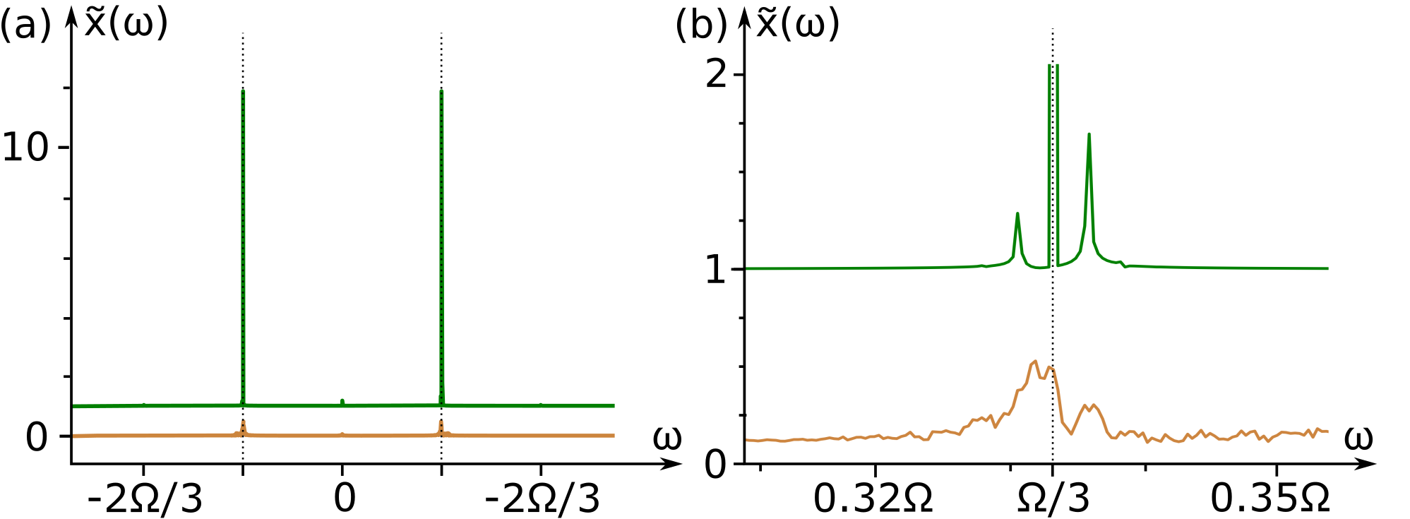
Figure 3: Observable signatures of quantum frequency locking. (a) Frequency spectrum of the cavity field, $\langle\hat{x}(t)\rangle$, for the system when initialized within (green), and outside (orange) the frequency locking regime, respectively. See main text for parameters and further details. Note that the green curve is vertically offset by $1$. (b) Zoom-in of panel (a), in the vicinity of $\omega=\Omega/3$ (indicated by vertical dashed line).

As a final goal for our numerical simulations, we explored the observable signatures of quantum frequency locking in the system, and their possible applications for frequency conversion. To this end, we considered the dynamics of the observable $\langle\hat{x}(t)\rangle$, which, depending on the exact realization of the model, for instance can measure a component of the electromagnetic field in the cavity (see Sec. II for definition). Using the parameters $\omega=0.34\Omega$, $\eta=0.56\Omega$ (also used in Figs. 1c and 2ac), we computed the time-evolution of the system after initializing the cavity mode in a coherent state with phase $0$ and displacement amplitude either $20$ or $10$, corresponding to locations $(x_{0},p_{0})=(20,0)$ and $(x_{0},p_{0})=(10,0)$ in phase-space. For both initializations we initialized the spin in the state $|\downarrow\rangle$, anti-aligned with the initial effective magnetic field ${\bf b}(x_{0},p_{0},0)$. From the resulting effective cavity Hamiltonian of the system shown in Fig. 2a, we expect these two initializations to place the system inside and outside the frequency locking regime, respectively.

In Fig. 3a, we show the dimensionless Fourier transform of $\langle\hat{x}(t)\rangle$ (absolute value), $|\tilde{x}(\omega)|$, for the two initializations above, while Fig. 3b shows a close-up of the spectrum in the vicinity of $\omega_{c}=\Omega/3$ [84]. In the frequency-locked regime, $|\tilde{x}(\omega)|$ features an extremely sharp peak of magnitude $\sim 10$ at $\omega=\Omega/3$. The two side-peaks visible in Fig. 3b arise from the slow orbit of the cavity wave-packet around the local minimum of $\mathcal{H}_{\rm eff}(x,p)$ (see Sec. III.1); their offset from the main peak defines the oscillation frequency of this motion. As is evident in Figs. 3cd, in the regime the system has a clear, measurable subharmonic response to the driving. In contrast, outside the frequency-locked regime, $|\tilde{x}(\omega)|$ shows a broad feature around the same value, but no well-defined peak.

When weakly coupled to an external environment (such as an electromagnetic waveguide), it may be possible to extract an output signal whose frequency spectrum shares the spectrum of $\langle x(t)\rangle$, and hence exhibits well-defined coherent oscillations at frequency $\Omega/q$ which is evident in Fig. 3 . In this way, the qubit-cavity system can potentially be exploited for frequency conversion.

VI Discussion

The discovery of Floquet time crystals sparked a broader investigation of discrete time-translation symmetry breaking. This work shows how such symmetry breaking can emerge as quantum frequency locking in a periodically driven spin-cavity system. When frequency-locked, the system exhibits well-defined oscillations with extended period ${\tilde{T}}=qT$, where $T$ denotes the driving period, and $q$ is an integer. Quantum frequency locking moreover has remarkable consequences for the quasienergy spectrum of a system: a large number of multiplets of Floquet eigenstates emerge whose quasi-energy differences are exponentially close to $n\Omega/q$ for $n=1,\ldots,q$. Using a semiclassical phase-space approach, we identify two mechanisms for frequency locking, which allow it to occur in a wide region of parameter space. Quantum frequency locking hence does not require fine-tuning, and can be reached through appropriately controlled but not fine-tuned initialization of the cavity mode, for a finite range of detuning $\delta\omega=\omega_{c}-r\Omega/q$, and for both weak and strong qubit-cavity coupling $\eta$.

The frequency locking exhibited by the qubit-cavity system is of fundamentally different nature than, e.g., time-crystalline behavior in spin chains (see, e.g., Refs. 14, 15). In the latter setting, time-translation symmetry breaking is also manifested in a large degeneracy of period-doubled Floquet eigenstates. However, for these systems, period multiplication emerges from the many-body nature of the system, and each quasienergy level in the system forms a part of a quasienergy-locked multiplet. In contrast, for the qubit-cavity system, only a finite (nonzero) number of quasienergy levels form multiplets.

We expect that the nontrivial fixed points of the stroboscopic motion generated by the semiclassical effective Hamiltonian $\mathcal{H}_{\rm eff}(x,p)$ remain stable in the presence of weak dissipation in the cavity, as would be the case if the radiation is allowed to leak out. In this case the frequency locking effect could be used for extracting an output signal whose frequency is given by a rational fraction of the drive, thus achieving frequency conversion. This offers an interesting direction for future studies.

The driven spin-cavity system we considered is perhaps one of the simplest systems that exhibits quantum frequency locking. This generic class of models can describe a diverse range of settings and physical systems, such as, e.g., Rydberg atoms in optical cavities and qubits in contact with microwave modes. Due to the simplicity of the model, and the many suitable experimental platforms, we expect that the qubit-cavity model forms a convenient and versatile platform for studying the breakdown of discrete time-translation symmetry. At strong coupling $\eta$, frequency locking moreover coexists with the topological energy-pumping regime that was analyzed in Ref. 17. Thus, the relatively simple and experimentally accessible model of a driven qubit-cavity system supports several distinct, highly nontrivial non-equilibrium phenomena. The simplicity of the platform, and the interplay of these nontrivial phenomena makes the driven qubit-cavity system an interesting subject for future experimental and theoretical studies.

Acknowledgements — IM was supported by the Materials Sciences and Engineering Division, Basic Energy Sciences, Office of Science, U.S. Dept. of Energy. FN and MR are grateful to the Villum Foundation and the European Research Council (ERC) under the European Union Horizon 2020 Research and Innovation Programme (Grant Agreement No. 678862) for support. GR is grateful for NSF DMR grant number 1839271. GR is also grateful to the U.S. Department of Energy, Office of Science, Basic Energy Sciences under Award DE-SC0019166. NSF and DOE supported GR’s time commitment to the project in equal shares.

Appendix A Photon lattice picture of frequency locking

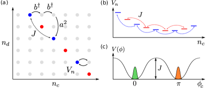
Figure 4: Photon lattice representation of frequency locking when drive $\Omega$ is close to $2\omega_{c}$. (a) Photon lattice of the system (see main text for details). Red and blue indicates the chain of sites along which the eigenstates of $H_{F}$ have their primary support when $\Omega\approx 2\omega_{c}$. Arrows indicate examples of resonant virtual processes contributing to the second nearest-neighbour tunneling $J$ and on-site potential $V_{n}$ of the effective tight-binding Hamiltonians of the chain. Different colors emphasize the decoupling into independent sublattices. (b) Schematic depiction of a tight-binding Hamiltonian for the chains, with sites and on-site potential shown as a function of $n_{c}$. (c) Energy profile as a function of the oscillator phase $\phi_{c}$ (variable conjugate to $n_{c}$), for the oscillator states close to the minimum of $V_{n}$. Green and orange are approximate bound states of the effective Hamiltonian near $\phi_{c}=0$ and $\pi$, each a superposition of “red” and “blue” chain states in (b). Up to exponentially weak tunneling correction, these bound states are also Floquet eigenstates, corresponding to the semiclassical states with the oscillator phases locked to $0$ or $\pi$ respectively.

In this appendix, we present a complementary perspective of frequency locking, based on the photon lattice picture of periodically driven systems. The approach is used to analyze frequency locking of the the qubit-cavity model in the limit of small anharmonicity $\eta$ and detuning. To demonstrate the emergence of frequency locking, we consider the case where the driving frequency is close to a rational multiple of the cavity frequency, $\Omega\approx q\omega_{c}/r$, where $q$ and $r$ are integers. We analyze the model as a periodically driven system with driving period ${\tilde{T}}=2\pi q/\Omega$ [recall that $H(t)=H(t+T)$ implies $H(t)=H(t+{\tilde{T}})$].

For a periodically driven system with driving period ${\tilde{T}}$, the photon lattice Hilbert space is spanned by the orthonormal basis $|i,n_{d}\rangle\!\rangle=|i\rangle\otimes|n_{d}\rangle$, where $i$ indexes the basis states of the original problem, while $n_{d}\in\mathbb{Z}$ can be seen as a lattice index, and heuristically counts the number of drive photons with energy $2\pi/{\tilde{T}}$ [85]. The extended Hilbert space Hamiltonian reads $H_{F}=\frac{2\pi}{{\tilde{T}}}\hat{n}_{d}+\sum_{z,w}H^{z}_{ij}|i,w+z\rangle\!\rangle\langle\!\langle j,w|,$ where $\hat{n}_{d}|i,n\rangle\!\rangle=n|i,n\rangle\!\rangle$, and $H_{ij}^{z}$ denotes the Fourier coefficients of $H_{ij}(t)$ (as a ${\tilde{T}}$-periodic function of time). One can verify that the eigenstates of $H_{F}$, $|\psi_{n}\rangle\!\rangle=\sum_{i,z}\psi^{n}_{i,z}|i,z\rangle\!\rangle$, are related to the Floquet eigenstates of $H(t)$ as follows:

$$|\psi_{n}\rangle=\sum_{i,z}\psi_{i,z}^{n}|i\rangle.$$ (20)

The quasienergy of the state $|\psi_{n}\rangle$ is related to the corresponding energy as $\varepsilon_{n}=E_{n}\,({\rm mod}\ 2\pi/qT)$. Note that each Floquet eigenstate of $H(t)$ corresponds to an infinite family of eigenstates of $H_{F}$ due to the symmetry $[\hat{a},H_{F}]=\frac{2\pi}{{\tilde{T}}},$ where $\hat{a}|i,n_{d}\rangle\!\rangle=|i,n_{d}-1\rangle\!\rangle$. As a result, if $|\psi_{n}\rangle\!\rangle$ is an eigenstate of $H_{F}$ with energy $E_{n}$, $\hat{a}|\psi_{n}\rangle\!\rangle$ is also an eigenstate of $H_{F}$, with energy $E_{n}-2\pi/(qT)$. Both eigenstates correspond to the same Floquet eigenstate through Eq. (20).

To find $H_{F}$ for the qubit-cavity system, we recall that the Hilbert space of the system is spanned by the states $|\alpha,n_{c}\rangle$, where $n_{c}=0,1,\ldots$ counts the number of cavity photons, while $\alpha=1,2$ denotes the state of the qubit. Hence, we can label the basis states for the extended Hilbert space $|\alpha,n_{c},n_{d}\rangle\!\rangle=|\alpha,n_{c}\rangle\otimes|n_{d}\rangle$. We write $H_{F}=V+K$ where $V$ and $K$ denote the diagonal and off-diagonal components in the basis above. To find $V$ and $K$, we recall from Eqs. (1)-(5) in the main text that the Hamiltonian $H(t)$ oscillates monochromatically with period $T$. Therefore, $H_{ij}^{z}$ is nonzero only when $z$ is an integer multiple of $q$. Equivalently, the above-introduced photon number shift operators $\hat{a}$ and $\hat{a}^{\dagger}$ only appear in powers of $q$ in the expression for $H_{F}$. Using the expression for $H(t)$ in Eqs. (1)-(5), we find

$$V = \hat{n}_{c}\omega_{c}+\frac{\Omega}{q}\hat{n}_{d}+\eta\sigma_{x}B_{0}$$ (21)

$$K = \frac{\eta A_{d}}{2}\left(\hat{a}^{q}[\sigma_{z}-i\sigma_{x}]+\hat{a}^{\dagger q}[\sigma_{z}+i\sigma_{x}]\right)+\eta(\hat{b}\sigma^{+}+\hat{b}^{\dagger}\sigma^{-}).$$

In the same way as for example in Refs. 16, 17, we can see $H_{F}$ as describing a $2D$ square lattice tight-binding model where $(n_{c},n_{d})$ denotes the site index in the “photon” lattice, and $\alpha$ denotes the orbital index. The sites in the photon lattice are coupled by the term $K$, and are subject to the on-site potential energy term $V$. Note that, by construction, the Hamiltonian $H_{F}=V+K$ only couples sites $(n_{c},n_{d})$ in the photon lattice separated by a distance $q$ in the second coordinate.

In the limit $\eta\to 0$, the term $V$ will generally dominate, and the eigenstates of $H_{F}$ are localized on individual sites in the photon lattice. The eigenstates are given by $|\Psi_{mn}^{\pm}\rangle\!\rangle\approx\frac{1}{\sqrt{2}}(|1,m,n\rangle\!\rangle\pm|2,m,n\rangle\!\rangle)$, with energies

$$E_{mn}^{\pm}=m\omega_{c}+\frac{n\Omega}{q}\pm\eta B_{0}.$$ (22)

These solutions are trivial, and hence typically there is no frequency locking in the small-$\eta$ limit. However, when the driving frequency $\Omega$ is sufficiently close to $\omega_{c}q/r$, the “potential energies” on sites $(n_{c},n_{d})$ and $(n_{c}+1,n_{d}-r)$ can be close enough that $K$ couples these sites resonantly through a high-order virtual processes (recall that the energy step size on the drive lattice as defined above is $\Omega/q$, while on the cavity lattice it is $\omega_{c}$). As a result, each eigenstate of $H_{F}$ may extend along a chain of sites $(k,b-rk)$ for $k=0,1,\ldots$, as depicted in Fig. 4a for the case $q/r=2$. Due to the symmetry of $H_{F}$ described below Eq. (20), there is just one independent chain ($b=0$), while the remaining chains are related by shifts in $n_{d}$.

Each chain is subject to an effective Hamiltonian which arises from the high-order virtual processes. This Hamiltonian takes the form

$$H_{\rm eff}=\sum_{m,n}|\alpha,m,-rm\rangle\!\rangle\langle\!\langle\beta,n,-rn|H^{\alpha\beta}_{mn}.$$ (23)

Here the matrix elements $H_{mn}^{\alpha\beta}$ can in principle be calculated analytically from perturbation theory in $\eta$. Since $H_{F}$ by construction only couples sites $(n_{c},n_{d})$ in the photon lattice separated by a distance $q$ in the second coordinate, the terms off-diagonal in photon number basis can only be nonzero when $m-n=kq$ for some integer $k$[86]. This coupling arises from virtual processes where $kp$ cavity photons are emitted, and $kq$ full drive photons (with frequency $\Omega$) are absorbed, or vice versa.

The above considerations show that the 1D chain model above itself separates into $q$ decoupled sublattices, distinguished by the value of $n_{c}\,({\rm mod}\ q)$. The tunneling coefficient $H_{m,m+kq}^{\alpha\beta}$ arises from a $k(q+r)$-th order virtual process (see Fig. 4a), and hence scales as $\eta^{k(q+r)}$. Thus, only the $k=1$ term is relevant in the $\eta\to 0$ limit. Following this discussion, we conclude that $H_{mn}^{\alpha\beta}$ takes the form

$$H_{mn}=V_{n}\delta_{mn}+\frac{1}{2}(J_{n}\delta_{m,n+q}+J^{\dagger}_{n}\delta_{n+q,m})$$ (24)

where $V_{n}$ and $J_{n}$ are $2\times 2$ matrices acting on the Hilbert space of the qubit, and we suppressed the qubit indices $\alpha,\beta$ for brevity. The term $V_{n}$ has contributions from the static field $B_{0}$, from the finite detuning $\delta\omega$, and from even-order “closed” virtual processes, while the origin of the term $J_{n}$ was discussed in the above.

While it is straightforward to analytically compute the terms $V_{n}$ and $J_{n}$ above through perturbation theory in $\eta$, such an analysis is beyond the scope of this paper. Instead, below we infer the emergence of frequency locking from a more qualitative discussion of the effective Hamiltonian above. We consider the case of a spinless model, where the coefficients $V_{n}$ and $J_{n}$ in Eq. (24) are scalars. Such a Hamiltonian emerges when the above line of arguments is applied to a periodically-driven anharmonic oscillator, such as considered in Ref. 42. We expect that the “spinful” model arising from the qubit-cavity system can be analyzed in a similar way.

To see how frequency locking arises in the spinless model, we note that for a finite range of detuning $\delta\omega=\omega-r\Omega/q$ the net potential energy $\tilde{V}_{n}=V_{n}+|J_{n}|$ may have a nontrivial minimum as a function of $n$, as schematically illustrated in Fig. 4c (the case of a maximum is similar). Near the minimum $n_{0}$ of $\tilde{V}_{n}$, to lowest order in $n-n_{0}$, $H$ takes the form

$$H_{mn}\approx\frac{k}{2}(n-n_{0})^{2}\delta_{mn}+\frac{J}{2}(\delta_{m,n+q}+\delta_{m,n-q}-2),$$ (25)

where $J=J_{n_{0}}$, and the “spring constant” $k$ can be computed from Taylor expanding $\tilde{V}_{n}$ around $n=n_{0}$. It is illuminating to express the Hamiltonian above in terms of the variable $\phi$ conjugate to $n-n_{0}$:

$$H_{\rm eff}=-\frac{1}{2m_{\rm eff}}\partial_{\phi}^{2}+J(\cos(q\phi)-1),$$ (26)

where $m_{\rm eff}=1/k$. Physically, since the index $n$ measures the value of $\hat{n}_{c}$ (i.e. the number of cavity mode photons) up to a constant shift by $n_{0}$ [see Eq. (23)], $\phi$ measures the phase of the cavity mode. Thus, when $n_{c}\approx n_{0}$ the effective Hamiltonian for the phase of the cavity mode describes the Hamiltonian of a free particle in a cosine potential $V(\phi)$ with well spacing $2\pi/q$ and depth $J$, as depicted in Fig. 4c.

Importantly, when the potential well depth $J$ is sufficiently large compared to the of kinetic energy of zero-point fluctuations associated with the effective mass $m_{\rm eff}$, the effective Hamiltonian above may support bound states where wave function of the system (as a function of $\phi$) is confined to one of the potential wells. In this state, with exponential accuracy, the phase of the oscillator $\phi$ is locked to an integer multiple of $2\pi/q$.

We now demonstrate that these bound states can be used to construct Floquet eigenstates of the qubit-cavity model where the phase has locked to the driving field [recall that the eigenstates in the photon lattice correspond to Floquet eigenstates of the qubit-cavity system through Eq. (20)]. Indeed, from the bound states $|\psi_{z}\rangle\!\rangle$ localized in isolated potential wells $z$, one can construct plane-wave” combinations, $|\Psi_{n}\rangle\!\rangle=\frac{1}{\sqrt{q}}\sum_{z}|\psi_{z}\rangle\!\rangle e^{-\frac{2\pi izn}{q}}$. Due to gaussian confinement of the wavefunction in the bottom of the near-harmonic potential wells in Eq. (26), the energy differences between these distinct combinations will be exponentially small in $\lambda^{2}/\xi^{2}$, where $\lambda=2\pi/q$ denotes the well separation, and $\xi=(Jm_{\rm eff})^{-1/4}$ denotes the scale of the phase fluctuations around the potential minimum.

Through the correspondence between eigenstates of $H_{F}$ and the Floquet eigenstates of the system, we conclude there must exist families of $q$ Floquet eigenstates, whose quasienergies differ by an integer multiple of $\Omega/q$, up to a correction $\delta\varepsilon$ exponentially small in $\lambda^{2}/\xi^{2}\sim\sqrt{Jm_{\rm eff}}/q^{2}$. This is in agreement with the main text, where we indeed found multiplets of Floquet eigenstates with exponentially close quasienergies modulo $\Omega/q$.

Appendix B Frequency locking at other frequency ratios

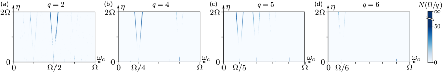
Figure 5: Number of period-$q$ frequency locking Floquet eigenstates as a function of $\omega_{c}$ and $\eta$, for the model depicted in Fig. 1c, for $q=2$ (a), $q=4$ (b), $q=5$ (c), and $q=6$(d). See Appendix B for further details.

Here we numerically demonstrate that quantum frequency locking also occurs at ratios other than $3$. For the same model and realizations studied in Sec. V (see Fig. 1c), we counted the number of frequency locking Floquet eigenstates at period multiplication $q$ for $q=2,4,5,6$, as a function of the coupling strength $\eta$ and cavity frequency $\omega_{c}$. The frequency locking states were identified from the quasienergy level spacings (modulo $\Omega/q$), in the same way as for the period-$3$ frequency locking states (see Sec. V). Our counting procedure identified a unique period multiplication for each frequency locking state, such that period-$2$ frequency locking eigenstates were not also double-counted as a period-4 Floquet eigenstates. In Fig. 5, we plot the obtained number of period-$q$ frequency locking states. (Note that a different color scale is used compared to Fig. 1, in order to heighten the contrast.) Fig. 5 clearly shows the same branch structure as Fig. 1c, with period-$q$ frequency locking occurring whenever $\omega_{c}/\Omega$ is close to $r/q$ for integer $r$. This demonstrates that period-$q$ frequency locking can occur for any $q$, when $\omega_{c}/\Omega$ is close enough to $r/q$ for some integer $r$.

Appendix C Derivation of $\mathcal{H}_{\rm eff}$ in Floquet regime

Here we identify the conditions for the Floquet regime, and derive the corresponding semiclassical effective Hamiltonian $\mathcal{H}_{\rm eff}(x,p)$ [Eqs. (8) and (16)]. These results were quoted in Sec. III.1.2 of the main text.

C.1 Conditions for the Floquet regime

We begin by deriving the conditions for the Floquet regime that we quoted in Sec. III.1.2, namely:

$$\eta\ll\theta(x,p)/\tilde{T},\quad\delta\omega\ll\tilde{\Omega}/A_{\rm cav}$$ (27)

where $\theta(x,p)$ denotes the stroboscopic precession angle (see sec. III.1.2), and $A_{\rm cav}\equiv\sqrt{x^{2}+p^{2}}$ denotes the displacement amplitude of the cavity mode.

To identify the conditions for Floquet locking, we consider the spin’s dynamics [Eq. (12) in the main text] for fixed $x$ and $p$. In this case ${\bf S}(t)$ evolves according to the Schrödinger-type equation

$$\partial_{t}S_{k}(t)=-i\sum_{l}H_{kl}^{(3)}(x,p,t){\bf S}_{l}(t),$$ (28)

where $H_{kl}^{(3)}(x,p,t)=-i\eta\sum_{j}h_{j}(x,p,t)\epsilon_{jkl}$ is a $3\times 3$ Hermitian matrix, with $\epsilon_{jkl}$ denoting the Levi-Civita tensor. Due to the Floquet theorem, Eq. (28) has $3$ complex-valued orthonormal solutions of the form ${\bf S}(t)={\bf n}_{j}(t)e^{-i\varepsilon_{j}t}$, where ${\bf n}_{j}(t)={\bf n}_{j}(t+{\tilde{T}})$. The antisymmetry of $H^{(3)}(t)$ implies that one of the stationary solutions is real-valued, with quasienergy zero. We identify this solution as the vector ${\bf n}_{0}(x,p,t)$ from Sec. III.1.2. Up to a prefactor, ${\bf n}_{0}(x,p,t)$ is the unique ${\tilde{T}}$-periodic solution to Eq. (12), with $x$ and $p$ fixed. The remaining two orthogonal solutions are related to each other by Hermitian conjugation, and have quasienergies $\pm\theta(x,p)/\tilde{T}$. The above properties imply that the effective Hamiltonian associated with $H^{(3)}(x,p,t)$ is given by

$$H_{\rm eff}^{\rm spin}(x,p)=[{\theta(x,p)}/{\tilde{T}}]{\bf a}(x,p)\cdot{\bf S},$$ (29)

where we used ${\bf n}_{0}(x,p,t)={\bf a}(x,p)$. Thus, we have related ${\bf a}(x,p)$, ${\bf n}_{0}(x,p,t)$ and $\theta(x,p)$ to the Floquet states and quasienergy spectrum of the $3\times 3$ antisymmetric Hamiltonian $H^{(3)}(x,p,t)$.

As quoted in Sec. III.1.2 (see also Ref. 78), the trajectory of the spin ${\bf S}(t)$ is locked to ${\bf n}_{0}(x(t),p(t),t)$ when the change of the stroboscopic precession axis ${\bf a}(x,p)={\bf n}_{0}(x,p,0)$ due to the motion of $x$ and $p$ is adiabatic with respect to the quasienergy gap of the effective spin Hamiltonian, $\delta\varepsilon(x,p)\equiv\frac{1}{\tilde{T}}\min(\theta(x,p),2\pi-2\theta(x,p))$:

$$\left|\frac{d}{dt}{\bf a}(x(t),p(t))\right|\ll\delta\varepsilon(x(t),p(t)),$$ (30)

where (with $x$, $p$, and $t$ suppressed)

$$\frac{d}{dt}{\bf a}=\dot{x}\partial_{x}{\bf a}+\dot{p}\partial_{p}{\bf a}.$$ (31)

To identify the conditions under which Eq. (30) holds, we thus need to bound $|\partial_{x}{\bf a}|$ and $|\partial_{p}{\bf a}|$.

To bound $\partial_{x}{\bf a}$, we consider the Floquet operator $R(x,p,{\tilde{T}})$, where $R(x,p,t)\equiv\mathcal{T}e^{-i\int_{0}^{t}\!{\rm d}t^{\prime}\,H^{(3)}(x,p,t^{\prime})}$ denotes the time-evolution operator generated by $H^{(3)}(x,p,t)$. Due to the antisymmetry of $H^{(3)}(x,p,t)$, $R(x,p,t)$ is an orthogonal matrix. Below we show through standard perturbative arguments that

$$|\partial_{x}{\bf a}|\leq\frac{2\|\partial_{x}R({\tilde{T}})\|}{\pi\delta\varepsilon(x,p){\tilde{T}}},$$ (32)

where $\left\lVert\cdot\right\rVert$ refers to the spectral norm, and $\delta\varepsilon(x,p)$ was defined above Eq. (30).

To prove Eq. (32), note that, since $R({\tilde{T}}){\bf a}={\bf a}$. Using the shorthand $R\equiv R(\tilde{T})$ here and below, we hence have $\partial_{x}(R{\bf a})=\partial_{x}{\bf a}$. Applying the chain rule, we also find $\partial_{x}(R{\bf a})=(\partial_{x}R){\bf a}+R\partial_{x}{\bf a}$. Equating these two expressions, we obtain

$$(\partial_{x}R){\bf a}=(1-R)\partial_{x}{\bf a}.$$ (33)

From the spectral decomposition of $R$, we have, for any vector ${\bf v}$, $|(1-R){\bf v}|\geq|e^{-i\delta\varepsilon T}-1||{\bf v}|$. Using this result along with $|e^{-i\alpha}-1|\geq\alpha\pi/2$ (for $\alpha\leq pi$) in the equation above, we obtain $|\partial_{x}R{\bf a}|\leq\delta\varepsilon{\tilde{T}}\pi|\partial_{x}{\bf a}|/2$. Using $|\partial_{x}R{\bf a}|\leq\left\lVert\partial_{x}R\right\rVert$, Eq. (32) follows.

Using the chain rule and the triangle inequality, one can verify $\|\partial_{x}R(x,p,{\tilde{T}})\|\leq\int_{0}^{{\tilde{T}}}{\rm dt}\|\partial_{x}H^{(3)}(x,p,t)\|$. Since $\|\partial_{x}H_{q}(x,p,t)\|\leq\eta|\partial_{x}{\bf h}|=\eta$, we then find $\|{\partial_{x}R(x,p,{\tilde{T}})}\|\leq\eta{\tilde{T}}.$ Thus, we conclude

$$|\partial_{x}{\bf a}|\leq\frac{2\eta}{\pi\delta\varepsilon(x,p)}.$$ (34)

The same bound holds for $|\partial_{p}{\bf a}|$ by similar arguments. Using the above result along with $\dot{x},\dot{p}\leq\eta+\delta\omega A_{\rm cav}$ [see Eqs. (10)-(11)] and the triangle inequality, we finally obtain

$$\left|\frac{d}{dt}{\bf a}\right|\leq\frac{4\eta}{\pi\delta\varepsilon(x,p)}(\eta+A_{\rm cav}\delta\omega).$$ (35)

Hence, using $4/\pi\sim 1$, the condition $|d{\bf a}/dt|\ll\delta\varepsilon$ is satisfied when

$$\delta\varepsilon^{2}\gg\eta^{2},\,\eta\delta\omega A_{\rm cav}.$$ (36)

Using $\delta\varepsilon\sim\theta(x,p)/\tilde{T}$, we see that the first condition above is equivalent to $\eta\ll\theta/\tilde{T}$, which is the first condition in Eq. (27). When $\delta\varepsilon\sim\theta(x,p)/\tilde{T}$, the second condition above ($\delta\varepsilon^{2}\gg\eta\delta\omega A_{\rm cav}$) is met if $\delta\omega\ll\theta/\tilde{T}A_{\rm cav}$; this is the second condition in Eq. (27). Thus the Floquet regime arises when the two conditions in Eq. (27) are satisfied. This was what we wanted to show.

C.2 Derivation of effective Hamiltonian

We now derive the effective Hamiltonian in Eqs. (8) and (16). In the Floquet regime, whose conditions were identified above, the discussion in Sec. III.1.2 implies that when the spin is initially aligned or anti-aligned with the stroboscopic precession axis, ${\bf S}(0)=\pm{\bf a}(x(0),p(0))$, the resulting evolution satisfies ${\bf S}(t)=\pm{\bf n}_{0}(x,p,t)$. Using this in Eqs. (10) and (11), we obtain

$$\dot{x}=v_{x}(x,p,t),\quad\dot{p}=-v_{p}(x,p,t),$$ (37)

where, for $s=x,p$,

$$v_{x}(x,p,t) \equiv \delta\omega p\pm\eta\partial_{p}{\bf h}(t)\cdot{\bf n}_{0}(x,p,t),$$ (38)

$$v_{p}(x,p,t) \equiv \delta\omega x\pm\eta\partial_{x}{\bf h}(t)\cdot{\bf n}_{0}(x,p,t).$$ (39)

When the conditions for the Floquet regime [Eq. (27)] are satisfied, the stroboscopic motion of the cavity mode is adiabatic; as a result, it can effectively be assumed stationary within a driving period. Hence, using the same arguments as in Sec. III.1.1 (see also Ref. [77]), we may integrate out the time-dependence of $v_{x}(x,p,t)$, obtaining

$$\dot{x}\approx\bar{v}_{x}(x,p),\quad\dot{p}\approx\bar{v}_{p}(x,p),$$ (40)

where, for $s=x,p$,

$$\bar{v}_{s}(x,p)=\delta\omega s\pm\frac{\eta}{{\tilde{T}}}\int_{0}^{{\tilde{T}}}\!\!\!{\rm d}t\,\partial_{s}{\bf h}(x,p,t)\cdot{\bf n}_{0}(x,p,t).$$ (41)

In the remainder of this subsection, we seek to show that $\bar{v}_{x}=\partial_{p}\mathcal{H}_{\rm eff}(x,p)$ and $\bar{v}_{p}=\partial_{x}\mathcal{H}_{\rm eff}(x,p)$, where $\mathcal{H}_{\rm eff}(x,p)$ is given in Eqs. (8) and (16) of the main text. To do this, we first use the chain rule to rewrite the integrand in the second term above for $s=p$ (the case $s=x$ follows analogously)

$$\partial_{p}{\bf h}\cdot{\bf n}_{0}=\partial_{p}\left[{\bf h}\cdot{\bf n}_{0}\right]-{\bf h}\cdot\partial_{p}{\bf n}_{0},$$ (42)

where we suppressed the above quantities’ dependence on $x$, $p$, and $t$ for brevity. We now consider the last term above. Since ${\bf n}_{0}$ obeys the Bloch equation [Eq. (12)] $\partial_{t}{\bf n}_{0}=-\eta{\bf h}\times{\bf n}_{0}$, we may write

$${\bf h}={\bf n}_{0}({\bf h}\cdot{\bf n}_{0})-\frac{1}{\eta}{\bf n}_{0}\times\partial_{t}{\bf n}_{0}.$$ (43)

This result can be proven by directly inserting $\partial_{t}{\bf n}_{0}=-\eta{\bf h}\times{\bf n}_{0}$ into the above, and using the cross product identity ${\bf a}\times({\bf b}\times{\bf c})={\bf b}({\bf a}\cdot{\bf c})-{\bf c}({\bf a}\cdot{\bf b})$ along with ${\bf n}_{0}\cdot{\bf n}_{0}=1$. Using the above result along with ${\bf n}_{0}\cdot\partial_{p}{\bf n}_{0}=0$ (recall that ${\bf n}_{0}$ is normalized), we obtain

$${\bf h}\cdot\partial_{p}{\bf n}_{0}=-\frac{1}{\eta}({\bf n}_{0}\times\partial_{t}{\bf n}_{0})\cdot\partial_{p}{\bf n}_{0}.$$ (44)

Using $({\bf a}\times{\bf b})\cdot{\bf c}={\bf b}\cdot({\bf c}\times{\bf a})$, and substituting into Eq. (C.2), we find

$$\partial_{p}{\bf h}\cdot{\bf n}_{0}=\partial_{p}\left[{\bf h}\cdot{\bf n}_{0}\right]+{\bf n}_{0}\cdot(\partial_{t}{\bf n}_{0}\times\partial_{p}{\bf n}_{0}).$$

We identify the second term as the the $x$-Berry flux $F_{x}(x,p,t)$ associated with the mapping of $\mathbb{R}^{3}$ to the unit sphere defined by ${\bf n}_{0}(x,p,t)$. One can verify that $\int_{0}^{{\tilde{T}}}\!{\rm d}t\,F_{x}(x,p,t)=\partial_{p}\gamma(x,p)$, where $\gamma(x,p)$ denotes the Berry phase associated with the loop traversed by ${\bf n}_{0}(x,p,t)$ on the unit sphere for $0\leq t<T$. Thus, we find

$$\frac{\eta}{{\tilde{T}}}\int_{0}^{{\tilde{T}}}\!\!\!{\rm d}t\,\partial_{p}{\bf h}\cdot{\bf n}_{0}=\frac{\partial}{\partial p}\left(\frac{\eta}{{\tilde{T}}}\int_{0}^{{\tilde{T}}}\!\!\!{\rm d}t\,{\bf h}\cdot{\bf n}_{0}+\frac{1}{{\tilde{T}}}\gamma\right).$$

Using this in Eq. (41), we obtain

$$\bar{v}_{x}(x,p)=\frac{\partial}{\partial p} \bigg{(}\frac{\delta\omega}{2}(x^{2}+p^{2})+\frac{1}{{\tilde{T}}}\gamma(x,p)$$

$$\pm\frac{\eta}{{\tilde{T}}}\int_{0}^{{\tilde{T}}}\!\!\!{\rm d}t\,{\bf h}(x,p,t)\cdot{\bf n}_{0}(x,p,t)\bigg{)},$$

where restored the dependence on $x$ and $p$ of the quantities above.

The final step is to show that the second term inside the parentheses above equals $\theta(x,p)/2\tilde{T}$. To show this, we recall that the Bloch equation $\partial_{t}{\bf S}(t)=-\eta{\bf h}(t)\times{\bf S}(t)$ describes the evolution of the expectation value of $\hat{{\bf S}}$ with the ${\tilde{T}}$-periodic spin-$1/2$ Hamiltonian $\hat{H}_{s}(t)=\eta{\bf h}(t)\cdot{\bf\hat{S}}$ (here we suppressed the dependence of ${\bf h}$ and $\hat{H}_{s}$ on $x$ and $p$). Noting that the stroboscopic time-evolution of $\langle{\bf S}\rangle$ is generated by a rotation by the angle $\varepsilon_{0}T$ around the axis ${\bf n}_{0}$ [see Eq. (29)], we conclude that the Floquet operator generated by $\hat{H}_{s}(t)$ is a $2\times 2$ unitary matrix given by $\hat{U}_{s}({\tilde{T}})=e^{-i\theta(x,p){\bf n}_{0}(0)\cdot{\bf\hat{S}}/2}$. Thus, we identify $\theta(x,p)/2\tilde{T}$ as the (positive) quasienergy associated with $\hat{H}_{s}(t)$.

To obtain an expression for $\varepsilon$, we note that $|\psi(t)\rangle=e^{-i\varepsilon t}|\phi_{+}(t)\rangle$ solves the Schrödinger equation generated by $\hat{H}_{s}(t)$, where $|\phi_{+}(t)\rangle$ denotes the Floquet state of $\hat{H}_{s}(t)$ with quasienergy $\varepsilon$. Thus, by direct substitution, one can verify that

$$\varepsilon=\frac{i}{{\tilde{T}}}\int_{0}^{{\tilde{T}}}\!\!\!\,{\rm d}t\,\langle\psi(t)|\partial_{t}|\psi(t)\rangle-\frac{i}{T}\int_{0}^{{\tilde{T}}}\!\!\!\,{\rm d}t\,\langle\phi_{+}(t)|\partial_{t}|\phi_{+}(t)\rangle.$$ (45)

We have $\langle\psi(t)|\partial_{t}|\psi(t)\rangle=i\eta{\bf n}(t)\cdot{\bf h}(t)$, where ${\bf n}(t)$ denotes the Bloch vector of the state $|\psi(t)\rangle$, which obeys the Bloch equation in Eq. (12). Note that ${\bf n}(t)$ is also identical to the Bloch vector of $|\phi_{+}(t)\rangle$. Since $|\phi_{+}(t)\rangle$ is time-periodic, ${\bf n}(t)$ is thus a time-periodic solution to the Bloch equation Eq. (12), and we identify ${\bf n}(t)={\bf n}_{0}(t)$ (the sign follows from the initial conditions). Identifying the latter term above as the Berry phase $\gamma(x,p)$ (with a factor of $1/{\tilde{T}}$), and restoring $x$ and $p$, we conclude

$$\frac{\theta(x,p)}{2\tilde{T}}=\frac{\eta}{{\tilde{T}}}\int_{0}^{{\tilde{T}}}\!\!\!{\rm d}t\,{\bf h}(x,p,t)\cdot{\bf n}_{0}(x,p,t)+\frac{1}{{\tilde{T}}}\gamma(x,p).$$ (46)

A similar result holds for $\bar{v}_{p}$. This was what we wanted to show, and concludes this Appendix.

Appendix D Derivation of quasienergy locking

In this Appendix, we show how quasienergy locking arises in the frequency-locked regime of the driven qubit-cavity system, using a more rigorous line of arguments than those presented in the main text. The discussion proceeds as follows: In Sec. D.1, we first consider the qualitative behavior of the qubit-cavity system in the regime. In Sec. D.2, by reconciling this behavior with Floquet eigenstate decomposition of the time-evolution (see Sec. IV.1), we conclude that such nontrivial extrema of $\mathcal{H}_{\rm eff}(x,p)$ implies the existence of multiplets of quasienergy levels of the form in Eq. (17) in the main text, whose corresponding Floquet states take the form in Eqs. (18)-(19).

D.1 Wavepacket dynamics in $q$-fold potential wells

To show how quasienergy locking arises, we consider the semiclassical effective Hamiltonian of the cavity mode in the regime, $\mathcal{H}_{\rm eff}(x,p)$ (see Sec. III.1); i.e., in the Floquet or adiabatic regimes, for parameters where $\mathcal{H}_{\rm eff}(x,p)$ acquires extrema at finite amplitude in phase space. As explained in Sec. IV.2 in the main text, $\mathcal{H}_{\rm eff}(x,p)$ has a built-in symmetry of discrete rotation by $2\pi/q$ in phase space. As a result, each potential well of this Hamiltonian (at finite displacement amplitude) forms part of a ring of $q$ potential wells that are related to each other through phase space rotations by $2\pi/q$.

We consider the rotating-frame time-evolution, $|\tilde{\psi}(t)\rangle$, of a wave packet $|\tilde{\psi}(0)\rangle$ initialized in one of the potential wells of $\mathcal{H}_{\rm eff}(x,p)$, referred to as well $0$ in the following. For example, $|\tilde{\psi}(0)\rangle$ may describe a direct-product state where the cavity mode is in a coherent state whose center in phase space $(x_{0},p_{0})$ is located in well $0$, while the spin is initialized along or against either ${\bf h}(x_{0},p_{0},0)$ (for the adiabatic regime) or ${\bf a}(x_{0},p_{0})$ (for the Floquet regime) [76]. Note that the corresponding initial state of the system in the lab frame, $|\psi(0)\rangle$, coincides with $|\tilde{\psi}(0)\rangle$ [see Sec. III.1]. Since $|\tilde{\psi}(t)\rangle$ must propagate along the constant-value contours of $\mathcal{H}_{\rm eff}(x,p)$, we expect that $|\tilde{\psi}(t)\rangle$ remains confined within well $0$ up to the timescale of quantum tunneling between the potential wells of $\mathcal{H}_{\rm eff}$, $\tau$. We expect the rate of quantum tunneling, $1/\tau$, to be exponentially suppressed in $d/\xi$, where $d$ denotes the separation between the potential wells in phase space, and $\xi\sim 1$ denotes the scale of quantum fluctuations. Hence, the duration of the confinement, $\tau$, scales exponentially with $d/\xi$.

We now consider the corresponding evolution of the system in the lab frame, $|\psi(t)\rangle$. We recall from Sec. III.1 that $|\psi(t)\rangle$ is obtained from $|\tilde{\psi}(t)\rangle$ through a phase space rotation by $2\pi rt/qT$. Hence, for integer $k$ where $k\ll\tau/T$, the support of $|\psi(kT)\rangle$ in the phase space (of the cavity mode) is confined to the potential well of $\mathcal{H}_{\rm eff}$ which is located at an angle $2\pi rk/q$ from well $0$ in phase space; we refer to this potential well as well $k$ in the following.

D.2 Implications for Floquet eigenstates

Above we showed that, in the quantum regime, the qubit-cavity system supports solutions that remain confined to potential well $k$ of $\mathcal{H}_{\rm eff}$ at time $t=kT$ (for integer $k$). The confinement persists for times $t\ll\tau$, where $\tau$ is the exponentially long timescale for tunneling between the potential wells of $\mathcal{H}_{\rm eff}$. In this section, we show how the resolvability of such a confined solution, $|\psi(t)\rangle$, in terms of Floquet eigenstates,

$$|\psi(kT)\rangle=\sum_{n}c_{n}e^{-i\varepsilon_{n}kT}|\psi_{n}\rangle,$$ (47)

dictates the behaviour of Floquet eigenstates and quasienergies of the system. Specifically, each Floquet eigenstate which significantly overlaps with $|\psi(0)\rangle$ must form a part of a multiplet of $q$ Floquet eigenstates of the form in Eq. (18) and (19), while the corresponding quasienergies are of the form in Eq. (17).

To simplify the analysis, we restrict the cavity mode’s phase space to the region where $|\psi(t)\rangle$ has its support: we let $r_{\rm max}$ denote the maximal distance $r$ from the origin in the cavity mode’s phase space where $|\psi(t)\rangle$ has significant support, and discard all states in the Hilbert space with more than $R^{2}$ photons of the cavity mode, for some $R\gg r_{\rm max}$. This truncation effectively discards the region of phase space located more than a distance $R$ from the origin; hence we do not expect it to significantly affect $|\psi(t)\rangle$. Moreover, we expect the Floquet eigenstates (and their corresponding quasienergies) to remain nearly unaffected by the truncation when they have full support well within a distance $R$ from the origin of phase space (up to exponentially small corrections). We assume $R$ can be chosen several orders of magnitude smaller than $(\tau/T)^{1/5}$, while still remaining much larger than $r_{\rm max}$. This is safe to assume since, as we recall from Sec. D.1, $\tau\sim e^{d/\xi}$ where $\xi\sim 1$ is the scale of quantum fluctuations, and $d$ the distance of the potential wells from the origin. In contrast, $r^{2}_{\rm max}$ only scales quadratically with $d/\xi$.

To characterize the properties of the Floquet eigenstates of the system with the truncated Hilbert space, we consider the stroboscopic time-evolution of the confined wavepacket, $|\psi(mT)\rangle$, for $m=0,1,\ldots N$ for some $N$. For sufficiently large $N$ (see below for specific conditions), we may use this to compute any Floquet eigenstate $|\psi_{n}\rangle$ whose overlap with the initial state, $c_{n}\equiv\langle\psi_{n}|\psi(0)\rangle$, is significant:

$$|\psi_{n}\rangle=\frac{1}{c_{n}N}\sum_{m=0}^{N}|\psi(mT)\rangle e^{im\varepsilon_{n}T}+\mathcal{O}([c_{n}N\delta\varepsilon_{n}T]^{-1}).$$ (48)

Here $\varepsilon_{n}$ denotes the quasienergy corresponding to $|\psi_{n}\rangle$, and $\delta\varepsilon_{n}\equiv\min_{m}|\varepsilon_{n}-\varepsilon_{m}|$ denotes the distance to the nearest adjacent quasienergy from $\varepsilon_{n}$. In the above, $\mathcal{O}(x)$ denotes a state with norm $\lesssim|x|$. The above result can be verified by direct insertion of Eq. (47) into the right-hand side above.

Since the truncated system has $2R^{2}$ quasienergy levels, uniformly distributed over the interval between $0$ and $\Omega$, the quasienergy spacing satisfies $\delta\varepsilon_{n}\sim\mathcal{O}([R^{2}T]^{-1})$. We refer to the overlap coefficient $c_{n}$ as being significant if $|c_{n}|\geq 1/\sqrt{2R^{2}}$ (at least one such Floquet eigenstate state should exist, due to the normalization of $|\psi(0)\rangle$ which implies $\sum_{n=1}^{2R^{2}}|c_{n}|^{2}=1$). Hence, for significantly overlapping Floquet eigenstates, the correction in Eq. (48) is, at most, of order $R^{3}/N$. We choose $N$ to be much smaller than, but still of same magnitude as $\tau/T$. With this choice, $N$ is much larger than $R^{3}$ (due to our assumption above that $R$ could be chosen much smaller than $(\tau/T)^{1/5}$, and $R>1$); hence for each significantly overlapping Floquet eigenstate $|\psi_{n}\rangle$, the correction in Eq. (48) is of order $\lesssim R^{3}T/\tau$, and hence much smaller than $1$.

Since we chose $N$ much smaller than $\tau/T$, for each $m$ between $0$ and $N$, $|\psi(mT)\rangle$ is still confined within well $m\,({\rm mod}\ q)$ of $\mathcal{H}_{\rm eff}(X,p)$. Thus $|\psi_{n}\rangle$ can be written as

$$|\psi_{n}\rangle=\sum_{k=1}^{q}|\chi^{k}_{n}\rangle+\mathcal{O}(R^{3}T/\tau),$$ (49)

where $|\chi_{n}^{k}\rangle$ consists of all terms in Eq. (48) where $m=k\,({\rm mod}\ q)$ and hence only has support only in potential well $k$ of phase space.

The states $\{|\chi_{n}^{k}\rangle\}$ transform nontrivially under time translation by one period: using that $\hat{U}(T)|\psi(mT)\rangle=|\psi([m+1]T)\rangle$, one can verify that

$$\hat{U}(T)|\chi_{n}^{k}\rangle=e^{-i\varepsilon_{n}T}|\chi_{n}^{k+1}\rangle+\mathcal{O}(R^{3}T/\tau),$$ (50)

where $|\chi^{q+1}_{n}\rangle=|\chi^{1}_{n}\rangle$. Due to their separate regions of support in phase space, the states $\{|\chi_{n}^{k}\rangle\}$ are mutually orthogonal. Since the right-hand side of Eq. (49) must have unit norm, the orthogonality of the states $\{|\chi_{n}^{k}\rangle\}$ along with Eq. (50) require that $\langle\chi_{n}^{k}|\chi_{n}^{k}\rangle=1/q+\mathcal{O}(R^{3}T/\tau)$ for each $k$.

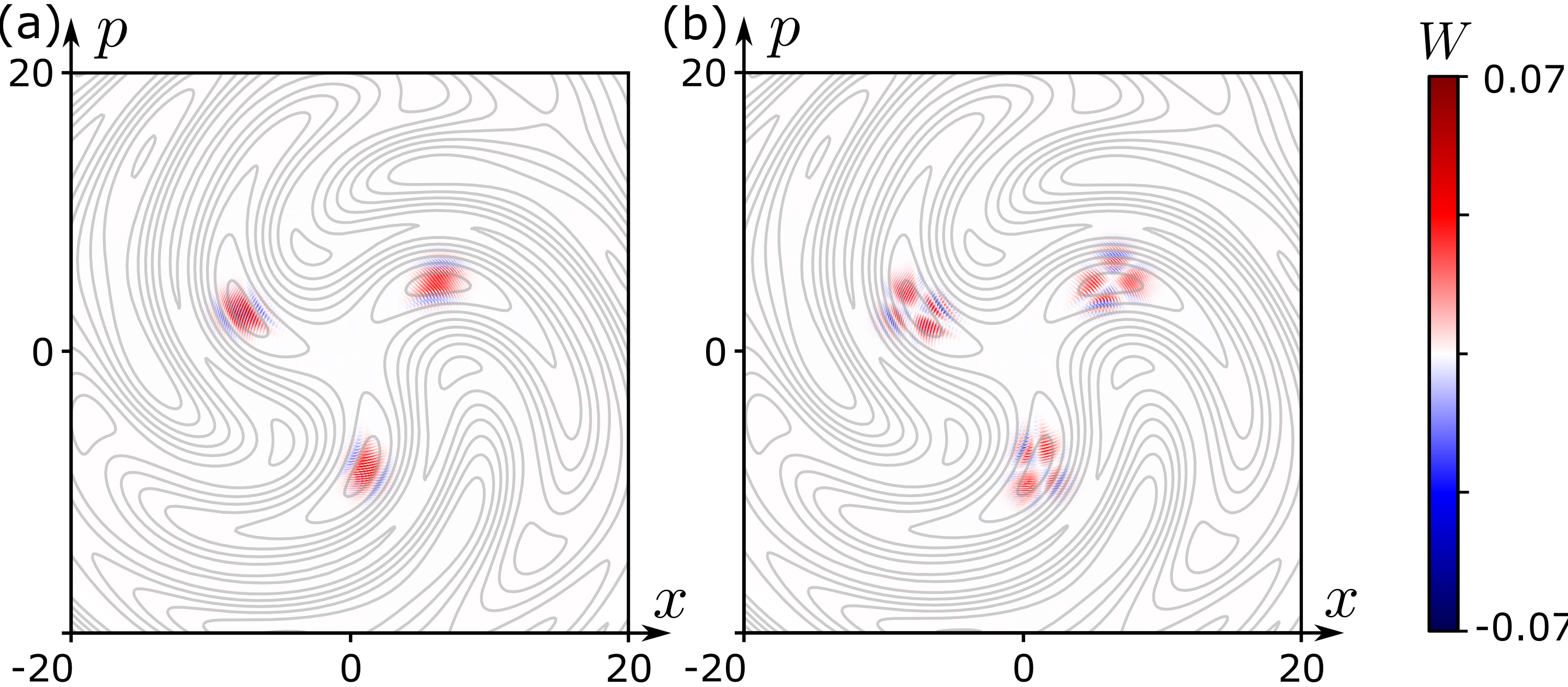
Figure 6: Wigner functions of two additional period-$3$ quasienergy-locked Floquet eigenstates for the same system as depicted in Fig. 2d, with support in a well distinct from the eigenstate in Fig. 2d.

We now use the states $\{|\chi^{k}_{n}\rangle\}$ to identify a family of Floquet eigenstates (including $|\psi_{n}\rangle$), whose quasienergies are separated from each other by integer multiples of $\Omega/q$ (up to corrections of order $1/\tau$) thus establishing the presence of quasienergy locking in the system. To this end, we consider the states $|\bar{\psi}_{n}^{1}\rangle,\ldots|\bar{\psi}_{n}^{q}\rangle$, where $|\bar{\psi}^{\ell}_{n}\rangle=\sum_{k=1}^{q}e^{-2\pi i\ell k/q}|\chi_{n}^{k}\rangle.$ Using Eq. (50), we see that

$$U(T)|\bar{\psi}^{\ell}_{n}\rangle=e^{-i(\varepsilon_{n}+\ell\Omega/q)T}|\bar{\psi}^{\ell}_{n}\rangle+\mathcal{O}(R^{3}T/\tau).$$ (51)

Moreover, $|\bar{\psi}^{\ell}_{n}\rangle$ has norm $1+\mathcal{O}(R^{3}T/\tau)$, due to the orthogonality and near-normalization of the states $\{|\chi_{k}^{n}\rangle\}$ [see text above Eq. (50)]. Thus, up to a correction of order $R^{3}T/\tau$, $|\bar{\psi}^{\ell}_{n}\rangle$ is a normalized Floquet eigenstate of the system. The existence of the approximate Floquet eigenstate $|\bar{\psi}_{n}^{\ell}\rangle$, along with the finite quasienergy level spacing, dictates [87] that there must exist an exact Floquet eigenstate of the system, $|\psi_{n}^{\ell}\rangle\approx|\bar{\psi}_{n}^{\ell}\rangle$ whose quasienergy is approximately given by $\varepsilon_{n}+\ell\Omega/q$. Specifically, $|\psi_{n}^{\ell}\rangle$ can be written

$$|\psi^{\ell}_{n}\rangle=\sum_{k=1}^{q}e^{-2\pi i\ell k/q}|\chi_{n}^{k}\rangle+\mathcal{O}(R^{5}T/\tau),$$ (52)

while the corresponding quasienergy is given by

$$\varepsilon_{n}+\ell\Omega/q+\mathcal{O}(R^{3}T/\tau).$$ (53)

For each Floquet eigenstate $|\psi_{n}\rangle$ that significantly overlaps with the state $|\psi(0)\rangle$ (according to the definition above), this construction can be made for each $\ell=1,\ldots q$ (note that $|\psi_{n}^{q}\rangle=|\psi_{n}\rangle$); hence, each Floquet eigenstate with significant support in the potential wells of $\mathcal{H}_{\rm eff}$ must form a part of a multiplet of $q$ Floquet states with the properties outlined in Eqs. (17)-(19) from the main text. This establishes the presence of quasienergy locking of the qubit-cavity system in the regimes, and concludes this Appendix.

Appendix E Floquet eigenstates with support in distinct potential wells

In this Appendix, we show Wigner functions for additional period-$3$ quasienergy-locked Floquet eigenstates of the qubit-cavity model for the parameters considered in Fig. 2bd (see main text for further details). These plots demonstrate that the distinct potential wells of $\mathcal{H}_{\rm eff}(x,p)$ for these parameters (see Fig 2b) support distinct triplets of quasienergy-locked Floquet eigenstates, and moreover that the same well may support several triplets.

In Fig. 6, we depict the Wigner functions for two quasienergy-locked Floquet eigenstates of the system distinct from the one depicted in Fig. 2d. Each of the Floquet eigenstates depicted in Fig. 6 form a part of its own triplet of quasienergy-locked Floquet eigenstates which, respectively, have (nearly) identical Wigner functions to the Wigner functions depicted in Fig. 6.

Note that the two Floquet eigenstates shown in Fig. 6 have support in the same well, and that this well is distinct from the one where the eigenstate shown in Fig. 2d has support. This confirms that the distinct potential wells of $\mathcal{H}_{\rm eff}(x,p)$ support distinct triplets of quasienergy locked Floquet eigenstates, and that the same well may support multiple triplets.

We finally note that the nodal lines of the Wigner functions in Fig. 6 coincide very closely with the contours of $\mathcal{H}_{\rm eff}(x,p)$ (gray lines), hence further supporting the discussion in Sec. III.1.

References

- Dalibard et al. [2011] J. Dalibard, F. Gerbier, G. Juzeliūnas, and P. Öhberg, Colloquium: Artificial gauge potentials for neutral atoms, Rev. Mod. Phys. 83, 1523 (2011).
- Eckardt [2017] A. Eckardt, Colloquium: Atomic quantum gases in periodically driven optical lattices, Rev. Mod. Phys. 89, 011004 (2017).
- Cooper et al. [2019] N. R. Cooper, J. Dalibard, and I. B. Spielman, Topological bands for ultracold atoms, Rev. Mod. Phys. 91, 015005 (2019).
- Oka and Kitamura [2019] T. Oka and S. Kitamura, Floquet engineering of quantum materials, Annual Review of Condensed Matter Physics, Annual Review of Condensed Matter Physics 10, 387 (2019).
- Rudner and Lindner [2020] M. S. Rudner and N. H. Lindner, Band structure engineering and non-equilibrium dynamics in Floquet topological insulators, Nat. Rev. Phys. 2, 229 (2020).
- Harper et al. [2019] F. Harper, R. Roy, M. S. Rudner, and S. L. Sondhi, Topology and broken symmetry in floquet systems (2019), arXiv:1905.01317 [cond-mat.str-el] .
- Oka and Aoki [2009] T. Oka and H. Aoki, Photovoltaic hall effect in graphene, Phys. Rev. B 79, 081406(R) (2009).
- Lindner et al. [2011] N. H. Lindner, G. Refael, and V. Galitski, Floquet topological insulator in semiconductor quantum wells, Nat. Phys. 7, 490 (2011).
- Jotzu et al. [2014] G. Jotzu, M. Messer, R. Desbuquois, M. Lebrat, T. Uehlinger, D. Greif, and T. Esslinger, Experimental realization of the topological haldane model with ultracold fermions, Nature 515, 237 (2014).
- Kitagawa et al. [2010] T. Kitagawa, E. Berg, M. Rudner, and E. Demler, Topological characterization of periodically driven quantum systems, Phys. Rev. B 82, 235114 (2010).
- Jiang et al. [2011] L. Jiang, T. Kitagawa, J. Alicea, A. R. Akhmerov, D. Pekker, G. Refael, J. I. Cirac, E. Demler, M. D. Lukin, and P. Zoller, Majorana Fermions in Equilibrium and in Driven Cold-Atom Quantum Wires, Phys. Rev. Lett. 106, 220402 (2011).
- Rudner et al. [2013] M. S. Rudner, N. H. Lindner, E. Berg, and M. Levin, Anomalous edge states and the bulk-edge correspondence for periodically driven two-dimensional systems, Phys. Rev. X 3, 031005 (2013).
- Titum et al. [2016] P. Titum, E. Berg, M. S. Rudner, G. Refael, and N. H. Lindner, Anomalous floquet-anderson insulator as a nonadiabatic quantized charge pump, Phys. Rev. X 6, 021013 (2016).
- Khemani et al. [2016] V. Khemani, A. Lazarides, R. Moessner, and S. L. Sondhi, Phase structure of driven quantum systems, Phys. Rev. Lett. 116, 250401 (2016).
- Else et al. [2016] D. V. Else, B. Bauer, and C. Nayak, Floquet time crystals, Phys. Rev. Lett. 117, 090402 (2016).
- Martin et al. [2017] I. Martin, G. Refael, and B. Halperin, Topological frequency conversion in strongly driven quantum systems, Phys. Rev. X 7, 041008 (2017).
- Nathan et al. [2019a] F. Nathan, I. Martin, and G. Refael, Topological frequency conversion in a driven dissipative quantum cavity, Physical Review B 99, 094311 (2019a).
- Crowley et al. [2019] P. J. D. Crowley, I. Martin, and A. Chandran, Topological classification of quasiperiodically driven quantum systems, Phys. Rev. B 99, 064306 (2019).
- Kolodrubetz et al. [2018] M. H. Kolodrubetz, F. Nathan, S. Gazit, T. Morimoto, and J. E. Moore, Topological floquet-thouless energy pump, Phys. Rev. Lett. 120, 150601 (2018).
- Nathan et al. [2019b] F. Nathan, D. Abanin, E. Berg, N. H. Lindner, and M. S. Rudner, Anomalous floquet insulators, Physical Review B 99, 195133 (2019b).
- Chandran and Sondhi [2016] A. Chandran and S. L. Sondhi, Interaction-stabilized steady states in the driven O(N) model, Phys. Rev. B 93, 174305 (2016).
- Po et al. [2016] H. C. Po, L. Fidkowski, T. Morimoto, A. C. Potter, and A. Vishwanath, Chiral Floquet Phases of Many-Body Localized Bosons, Physical Review X 6, 041070 (2016).
- Reiss et al. [2018] D. Reiss, F. Harper, and R. Roy, Interacting Floquet topological phases in three dimensions, Phys. Rev. B 98, 045127 (2018).
- Potter et al. [2018] A. C. Potter, A. Vishwanath, and L. Fidkowski, Infinite family of three-dimensional Floquet topological paramagnets, Phys. Rev. B 97, 245106 (2018).
- Yao et al. [2017] N. Yao, A. Potter, I.-D. Potirniche, and A. Vishwanath, Discrete time crystals: Rigidity, criticality, and realizations, Physical Review Letters 118, 030401 (2017).
- Else et al. [2017] D. V. Else, B. Bauer, and C. Nayak, Prethermal Phases of Matter Protected by Time-Translation Symmetry, Physical Review X 7, 011026 (2017).
- Iemini et al. [2018] F. Iemini, A. Russomanno, J. Keeling, M. Schirò, M. Dalmonte, and R. Fazio, Boundary Time Crystals, Phys. Rev. Lett. 121, 035301 (2018).
- Nurwantoro et al. [2019] P. Nurwantoro, R. W. Bomantara, and J. Gong, Discrete time crystals in many-body quantum chaos, Phys. Rev. B 100, 214311 (2019).
- Khemani et al. [2017] V. Khemani, C. W. von Keyserlingk, and S. L. Sondhi, Defining time crystals via representation theory, Phys. Rev. B 96, 115127 (2017).
- Huang et al. [2018] B. Huang, Y.-H. Wu, and W. V. Liu, Clean Floquet Time Crystals: Models and Realizations in Cold Atoms, Phys. Rev. Lett. 120, 110603 (2018).
- Autti et al. [2018] S. Autti, V. B. Eltsov, and G. E. Volovik, Observation of a Time Quasicrystal and Its Transition to a Superfluid Time Crystal, Phys. Rev. Lett. 120, 215301 (2018).
- Bello et al. [2019] L. Bello, M. Calvanese Strinati, E. G. Dalla Torre, and A. Pe’er, Persistent Coherent Beating in Coupled Parametric Oscillators, Phys. Rev. Lett. 123, 083901 (2019).
- Cosme et al. [2019] J. G. Cosme, J. Skulte, and L. Mathey, Time crystals in a shaken atom-cavity system, Phys. Rev. A 100, 053615 (2019).
- Zhu et al. [2019] B. Zhu, J. Marino, N. Y Yao, M. D. Lukin, and E. A. Demler, Dicke time crystals in driven-dissipative quantum many-body systems, New Journal of Physics 21, 073028 (2019).
- Gong et al. [2018] Z. Gong, R. Hamazaki, and M. Ueda, Discrete time-crystalline order in cavity and circuit qed systems, Phys. Rev. Lett. 120, 040404 (2018).
- Barberena et al. [2019] D. Barberena, R. J. Lewis-Swan, J. K. Thompson, and A. M. Rey, Driven-dissipative quantum dynamics in ultra-long-lived dipoles in an optical cavity, Phys. Rev. A 99, 053411 (2019).
- Broome et al. [2010] M. A. Broome, A. Fedrizzi, B. P. Lanyon, I. Kassal, A. Aspuru-Guzik, and A. G. White, Discrete single-photon quantum walks with tunable decoherence, Phys. Rev. Lett. 104, 153602 (2010).
- Sacha [2015] K. Sacha, Modeling spontaneous breaking of time-translation symmetry, Phys. Rev. A 91, 033617 (2015).
- Hu et al. [2015] W. Hu, J. C. Pillay, K. Wu, M. Pasek, P. P. Shum, and Y. D. Chong, Measurement of a Topological Edge Invariant in a Microwave Network, Phys. Rev. X 5, 011012 (2015).
- von Keyserlingk and Sondhi [2016] C. W. von Keyserlingk and S. L. Sondhi, Phase structure of one-dimensional interacting Floquet systems. II. Symmetry-broken phases, Phys. Rev. B 93, 245146 (2016).
- Choi et al. [2017] S. Choi, J. Choi, R. Landig, G. Kucsko, H. Zhou, J. Isoya, F. Jelezko, S. Onoda, H. Sumiya, V. Khemani, C. von Keyserlingk, N. Y. Yao, E. Demler, and M. D. Lukin, Observation of discrete time-crystalline order in a disordered dipolar many-body system, Nature 543, 221 (2017).
- Zhang et al. [2017] Y. Zhang, J. Gosner, S. M. Girvin, J. Ankerhold, and M. I. Dykman, Time-translation-symmetry breaking in a driven oscillator: From the quantum coherent to the incoherent regime, Phys. Rev. A 96, 052124 (2017).
- Maczewsky et al. [2017] L. J. Maczewsky, J. M. Zeuner, S. Nolte, and A. Szameit, Observation of photonic anomalous Floquet topological insulators, Nature Comm. 8, 13756 (2017).
- Mukherjee et al. [2017] S. Mukherjee, A. Spracklen, M. Valiente, E. Andersson, O. Ohberg, N. Goldman, and R. R. Thomson, Experimental observation of anomalous topological edge modes in a slowly-driven photonic lattice, Nature Comm. 8, 13918 (2017).
- Moessner and Sondhi [2017] R. Moessner and S. L. Sondhi, Equilibration and order in quantum Floquet matter, Nat. Phys. 13, 424 (2017).
- Ho et al. [2017] W. W. Ho, S. Choi, M. D. Lukin, and D. A. Abanin, Critical Time Crystals in Dipolar Systems, Phys. Rev. Lett. 119, 010602 (2017).
- Russomanno et al. [2017] A. Russomanno, F. Iemini, M. Dalmonte, and R. Fazio, Floquet time crystal in the lipkin-meshkov-glick model, Phys. Rev. B 95, 214307 (2017).
- McIver et al. [2019] J. W. McIver, B. Schulte, F.-U. Stein, T. Matsuyama, G. Jotzu, G. Meier, and A. Cavalleri, Light-induced anomalous hall effect in graphene, Nature Physics 16, 38 (2019).
- Choi et al. [2019] J. Choi, H. Zhou, S. Choi, R. Landig, W. W. Ho, J. Isoya, F. Jelezko, S. Onoda, H. Sumiya, D. A. Abanin, and M. D. Lukin, Probing quantum thermalization of a disordered dipolar spin ensemble with discrete time-crystalline order, Phys. Rev. Lett. 122, 043603 (2019).
- Wintersperger et al. [2020] K. Wintersperger, C. Braun, F. N. Ünal, A. Eckardt, M. D. Liberto, N. Goldman, I. Bloch, and M. Aidelsburger, Realization of an anomalous floquet topological system with ultracold atoms, Nature Physics 16, 1058 (2020).
- Holthaus and Flatté [1994] M. Holthaus and M. E. Flatté, Subharmonic generation in quantum systems, Physics Letters A 187, 151 (1994).
- Sacha and Zakrzewski [2017] K. Sacha and J. Zakrzewski, Time crystals: a review, Rep. Prog. Phys. 81, 016401 (2017).
- Giergiel et al. [2018] K. Giergiel, A. Kosior, P. Hannaford, and K. Sacha, Time crystals: Analysis of experimental conditions, Phys. Rev. A 98, 013613 (2018).
- Pizzi et al. [2019] A. Pizzi, J. Knolle, and A. Nunnenkamp, Period- discrete time crystals and quasicrystals with ultracold bosons, Phys. Rev. Lett. 123, 150601 (2019).
- Matus and Sacha [2019] P. Matus and K. Sacha, Fractional time crystals, Phys. Rev. A 99, 033626 (2019).
- [56] In Fig. 1c, quantum frequency locking occurs for a nonzero range of driving frequencies for any given value of . Hence we expect that it is enough to have good control over a single parameter (such as the driving frequency) to reach a regime where quantum frequency locked occurs. We expect this to be achievable in experiments.
- Surace et al. [2019] F. M. Surace, A. Russomanno, M. Dalmonte, A. Silva, R. Fazio, and F. Iemini, Floquet time crystals in clock models, Phys. Rev. B 99, 104303 (2019).
- Huang et al. [2020] Z. Huang, A. Clerk, and I. Martin, Non-dispersing wave packets in lattice floquet systems, arXiv preprint arXiv:2005.08993 (2020).
- Guo et al. [2013] L. Guo, M. Marthaler, and G. Schön, Phase space crystals: A new way to create a quasienergy band structure, Phys. Rev. Lett. 111, 205303 (2013).
- Gross and Bloch [2017] C. Gross and I. Bloch, Quantum simulations with ultracold atoms in optical lattices, Science 357, 995 (2017).
- Burkard et al. [2020] G. Burkard, M. J. Gullans, X. Mi, and J. R. Petta, Superconductor–semiconductor hybrid-circuit quantum electrodynamics, Nature Reviews Physics 2, 129 (2020).
- Clerk et al. [2020] A. A. Clerk, K. W. Lehnert, P. Bertet, J. R. Petta, and Y. Nakamura, Hybrid quantum systems with circuit quantum electrodynamics, Nature Physics 16, 257 (2020).
- Rasband [1990] S. N. Rasband, Chaotic Dynamics of Nonlinear Systems (John Wiley and Sons, 1990).
- Strogatz [2001] S. Strogatz, Nonlinear Dynamics And Chaos: With Applications To Physics, Biology, Chemistry, And Engineering (Studies in Nonlinearity) (Westview Press, 2001).
- Jessop et al. [2020] M. R. Jessop, W. Li, and A. D. Armour, Phase synchronization in coupled bistable oscillators, Phys. Rev. Research 2, 013233 (2020).
- Tan and Gabrielse [1991] J. Tan and G. Gabrielse, Synchronization of parametrically pumped electron oscillators with phase bistability, Phys. Rev. Lett. 67, 3090 (1991).
- Buchleitner et al. [2002] A. Buchleitner, D. Delande, and J. Zakrzewski, Non-dispersive wave packets in periodically driven quantum systems, Physics Reports 368, 409 (2002).
- Lörch et al. [2019] N. Lörch, Y. Zhang, C. Bruder, and M. I. Dykman, Quantum state preparation for coupled period tripling oscillators, Physical Review Research 1, 10.1103/physrevresearch.1.023023 (2019).
- [69] Specifically, and are normalized such that gives the number of photons in the cavity mode.
- Manucharyan et al. [2009] V. E. Manucharyan, J. Koch, L. I. Glazman, and M. H. Devoret, Fluxonium: Single cooper-pair circuit free of charge offsets, Science 326, 113 (2009).
- Nguyen et al. [2019] L. B. Nguyen, Y.-H. Lin, A. Somoroff, R. Mencia, N. Grabon, and V. E. Manucharyan, High-coherence fluxonium qubit, Phys. Rev. X 9, 041041 (2019).
- Childress et al. [2006] L. Childress, M. V. G. Dutt, J. M. Taylor, A. S. Zibrov, F. Jelezko, J. Wrachtrup, P. R. Hemmer, and M. D. Lukin, Coherent Dynamics of Coupled Electron and Nuclear Spin Qubits in Diamond, Science 314, 281 (2006).
- Sushkov et al. [2014] A. O. Sushkov, I. Lovchinsky, N. Chisholm, R. L. Walsworth, H. Park, and M. D. Lukin, Magnetic resonance detection of individual proton spins using quantum reporters, Phys. Rev. Lett. 113, 197601 (2014).
- Bentsen et al. [2019] G. Bentsen, I.-D. Potirniche, V. B. Bulchandani, T. Scaffidi, X. Cao, X.-L. Qi, M. Schleier-Smith, and E. Altman, Integrable and chaotic dynamics of spins coupled to an optical cavity, Phys. Rev. X 9, 041011 (2019).
- Kroeze et al. [2018] R. M. Kroeze, Y. Guo, V. D. Vaidya, J. Keeling, and B. L. Lev, Spinor self-ordering of a quantum gas in a cavity, Phys. Rev. Lett. 121, 163601 (2018).
- [76] For a more general initialization of the spin, the initial state can always be decomposed as a superposition of two states where the spin is aligned and anti-aligned with the initial effective precession axis (i.e., and for the adiabatic and Floquet regime, respectively). The two components can be analyzed separately using the arguments in Sec. III.1. Since the cavity mode experiences different effective Hamiltonians for the two components, we expect the evolution of the state to consist of a superposition of two distinct semiclassical trajectories of the cavity mode, as was observed in Ref. [17].
- Oteo and Ros [1991] J. A. Oteo and J. Ros, The Magnus expansion for classical Hamiltonian systems, J. Phys. A 24, 5751 (1991).
- Weinberg et al. [2017] P. Weinberg, M. Bukov, L. D’Alessio, A. Polkovnikov, S. Vajna, and M. Kolodrubetz, Adiabatic perturbation theory and geometry of periodically-driven systems, Physics Reports 688, 1 (2017).
- [79] To see this, note that .
- [80] Note that for any quasienergy-locked system there exists an infinite number of ways to construct a family of orthogonal states that satisfy Eqs. (18) and (19). Such distinct families can be obtained by modifying the (arbitrary) phase factor in front of each eigenstate in the expression for below Eq. (18). However, for the qubit-cavity system we consider in this work, there exists a unique way to assign phase factors to the Floquet eigenstates (up to an overall common phase factor), such that each has support only in a particular well of in phase space. We expect analogous results hold for other realizations of quasienergy locking.
- [81] This follows since the Floquet operator in the rotating frame, , is given by , where denotes the Floquet operator in the lab frame (recall that , while ).
- [82] Note that the same ring of potential wells can support multiple families of quasienergy-locked eigenstates if an individual potential well in the ring supports multiple bound states, as demonstrated in Appendix E.
- [83] Since , and does not transfer out of well in the frequency locked regime, approximately generates a phase space rotation by . Moreover note that by construction is a symmetry of the exact effective Hamiltonian in the rotating frame, , regardless of any approximations.
- [84] Specifically, . The data in Fig. 3cd are computed using .
- Shirley [1965] J. H. Shirley, Solution of the schrödinger equation with a hamiltonian periodic in time, Physical Review 138, B979 (1965).
- [86] Specifically, the inherent structure of implies that terms in Eq. (23) can only be nonzero if for some integer . Since is an irreducible fraction, this can only be true if for some integer . As a result, sites and are coupled only when .
- [87] To see this, note that implies that the smallest eigenvalue of must have absolute value less than . Moreover, we note that the component of orthogonal to the corresponding eigenstate must be of order , where was defined below Eq. (48).