Tidal effects in the motion of gas clouds around boson stars

Abstract

We study the motion of gas clouds in the vicinity of boson stars, performing simulations with the Black Hole Accretion Code BHAC. We compare the motion of the gas clouds with particle motion along geodesics and analyze the tidal effects on the gas clouds, which leads to disruption of the clouds. First we consider small and dense clouds associated with three different types of bound orbits close to the boson star and analyze the mechanisms of debris formation for these. We infer from the simulations that the lifetimes of these nearby clouds are longer for initially circularly orbiting clouds than for clouds on initially eccentric orbits. Next we compare the evolution of more extended and less dense clouds on initially circular orbits around a boson star and a Schwarzschild black hole and compare the motion in these two spacetimes. In particular, we observe the formation of a ring-like structure around the boson star endowed with a spiralling shock structure and a constant thermal bremsstrahlung total luminosity. This final configuration contrasts strongly with the black hole scenario where the gas is totally captured behind the event horizon.

I Introduction

In recent years black holes have featured most prominently in astrophysical observations. On the one hand, the LIGO/VIRGO collaboration has detected gravitational waves produced in the powerful merger events of stellar black holes, giving even rise to an intermediate size black hole (see e.g. [1, 2, 3]). On the other hand, the EHT collaboration has presented observations of the shadow and the accretion disk for the supermassive compact object at the center of the galaxy M87 [4, 5, 6, 7, 8, 9]. Notwithstanding, over the course of two decades the MPE and UCLA teams have collected data, observing stars’ motion in the vicinity of Sagittarius A*, which strongly suggests that at the center of our Milky Way galaxy dwells a supermassive black hole. [10, 11, 12, 13, 14, 15, 16].

Still, the case for possible contenders of black holes is not yet closed, leaving the need to scrutinize these further. Exotic compact objects warp spacetime in such a manner that it is regular everywhere and no horizon is formed. However, since they may possess a high compactness, ergospheres and photon spheres may arise, letting these objects act as black hole mimickers. For instance, the gravitational wave spectrum of the ringdown phase of exotic compact objects can be initially almost identical to the one of a black hole [17, 18].

First studied in the late 60’s [19, 20, 21] boson stars (BSs) are formed by a complex scalar field bound by gravity, and hence BSs seem a rather attractive candidate for exotic compact objects. In fact, their sizes can range from the atomic scale to the scale of supermassive black holes (BHs). Thus such a supermassive BS might well dwell at the center of our very own galaxy [22, 23, 24]. Albeit the simplicity of this type of matter fields, the resulting physics is extremely interesting, mainly because of the stars’ features that differ enormously from those of other final state systems such as BHs or neutron stars. The generated spacetime is asymptotically flat, but the scalar field becomes only trivial at spatial infinity, and the star possesses therefore no clear boundary that could be identified with its surface where the pressure vanishes. Yet the investigation of BSs as realistic contenders of astrophysical relevance lies in the fact that the complex scalar field only interacts gravitationally with ordinary matter, which can freely orbit in the stars’ interior all the way to the core with no resistance from the bosonic field.

The theory underlying the existence of BSs is endowed with a global $U(1)$ symmetry, and thus possesses a conserved Noether current and associated charge $N$, understood as the particle number. It is also possible to promote this symmetry to a local one by gauging the scalar field, which then sources an electromagnetic-like field [25]. Rotating BS solutions were first obtained in the 90’s, after the perturbative approach proved to be of no avail [26]. The underlying reason is that the angular momentum of rotating BSs is quantized in units of the particle number, $J=mN$ (with $m\in\mathbb{Z}$) [27, 28]. Solving the full nonlinear set of partial differential equations numerically, numerous sets of rotating BSs were obtained and analyzed, including their stability, excitations, existence also in higher dimensions and generalizaton to multistate BSs, reflecting the richness of their nature in a plethora of different configurations [29, 30, 31, 32, 33, 34, 35, 36, 37, 38, 39].

Geodesic motion of test particles in BS spacetimes has been studied in [40, 41, 42, 43, 44, 45, 46], where unusual types of orbits have been found, not present in Schwarzschild or Kerr BH spacetimes, such as the semi orbit, the pointy petal orbit and the static ring. The latter represents a set of orbits, where a particle at rest with respect to an asymptotic static observer remains at rest in a static orbit [46]. The investigation of the circular orbits of particles in BS spacetimes has also revealed distinct features as compared to BH spacetimes. Whereas BH spacetimes feature ISCOs, i.e., innermost stable circular orbits, where a change of stability occurs, boson stars feature ICOs, i.e., innermost circular orbits, beyond which no circular motion is possible [42, 43, 47].

Circular orbits are of particular importance in the study of accretion disks around compact objects. Regarding thick tori around BSs, Meliani et al. [43] have reported important differences between those in the BS and BH context, by exploring analytical solutions of stable circular fluid configurations and their evolution through simulations. Olivares et al. [49] have explored magnetized tori together with general-relativistic radiative-transfer calculations, pointing out also potential differences in the appearance of BSs and BHs. Also, the iron K$\alpha$ line of thin accretion disks around mini BSs has been analyzed [52] and found to be in most cases incompatible with current x-ray data from BH binaries. However, compatibility with the data might change dramatically for compact BSs, composed of self-interacting fields.

The motion of gas clouds around rotating BSs has been studied in [48], where simulations have been performed for near-by and far away clouds. Under the influence of the gravitational field from the BSs, these clouds have been tidally distorted and disrupted. For the two regimes of near-by and far away clouds major differences were found. While for clouds falling into the BSs from a great distance the formation of a torus-like structure inside the BSs was reported, the near-by clouds were capable to retain largely their shape.

In the present paper we shall also address the motion and distortion of gas clouds, but in the context of non-rotating compact BSs. Unlike the clouds considered in [48], the clouds reported here also do not necessarily start at rest with respect to a zero angular momentum observer at infinity. In fact, without the Lense-Thirring effect, in order to explore angular motion of the gas, initial angular momentum of the clouds is required. Our simulations are then performed in two regimes, consisting of dense small clouds with orbits close to the BSs and more extended and less dense clouds further away from the BSs. The former allows us to distinguish between the gas motion and the particle geodesic motion, thereby finding the debris formation mechanism, while the latter is meant to compare the evolution around a BS with that of a BH, as well as to investigate the possibility for disk formation. In both regimes we have considered the total mass of the clouds to be much smaller than the mass of the central compact object. This assumption obviates the necessity of defining a tidal radius since the self-gravity of the clouds will not be considered.

Following an analogous approach to Meliani et al. [48], we restrict our analysis to the 2D case. Accordingly, the thickness of the cloud is neglected, as well as any component of the dynamical quantities orthogonal to the cloud’s plane. Such a restriction is compatible with the nature of the spherically symmetric spacetimes analysed, and valid as a preliminary approach to the dynamics of the clouds. Indeed, important features such as the vertical mode of the magneto rotational instability (MRI) turbulence are irrelevant since we are not considering the presence of magnetic fields. Also, although vertical velocity components would contribute to the pressure oscillations observed, such contributions are not expected to divert our results, when considering the gas to be symmetric with respect to the equatorial plane chosen.

This paper is structured in the following format. In sections 2 and 3 we shall describe, respectively, the BS model employed and the numerical method together with the simulation setup. Sections 4 and 5 describe and discuss the simulations, while section 6 presents our conclusions.

II Boson star model

Boson stars are obtained by minimally coupling a complex scalar field to gravity. The action of the system is given by

$$S=\int\Big{[}\frac{\cal{R}}{16\pi G}-\frac{1}{2}g^{\mu\nu}\left(\partial_{\mu}\Phi\partial_{\nu}\Phi^{*}+\partial_{\nu}\Phi\partial_{\mu}\Phi^{*}\right)$$

$$-U\left(\lvert\Phi\rvert\right)\Big{]}\sqrt{-g}d^{4}x,$$ (1)

where ${\cal R}$ is the curvature scalar, $G$ is Newton’s constant, $g^{\mu\nu}$ is the inverse metric, $\Phi$ is the complex scalar field, $U$ is the self-interaction potential, and $g$ is the metric determinant. The model has a U(1) invariance with conserved current $j^{\mu}=-i(\Phi^{*}\partial^{\mu}\Phi-\Phi\partial^{\mu}\Phi^{*})$. Boson stars could form thanks to a phenomenon known as gravitational cooling, which is dissipationless and similar to the violent relaxation of collisionless stellar systems, but yet more efficient, i.e. even for high ratios between kinetic and potential energy a compact object is formed by ejecting scalar material carrying away the exceeding energy, and this final state is quite insensitive to the initial conditions [50, 51].

We vary the action with respect to the metric and the scalar field to obtain the Einstein field equations and a Klein-Gordon equation, respectively. We then employ the usual spherically symmetric ansatz, where the scalar field has a harmonic time-dependence $\Phi=\phi(r)\exp{(i\omega_{s}t)}$, and the line element reads

$$ds^{2}=-e^{f(r)}dt^{2}+e^{l(r)}dr^{2}+r^{2}d\Omega^{2},$$ (2)

to obtain a system of three coupled ODEs, namely

$$l^{\prime}=\phi^{\prime 2}r^{2}+e^{l-f}\omega_{s}^{2}\phi^{2}r+\frac{1}{r}\left(e^{l}-1\right)-e^{l}Ur,$$ (3)

$$f^{\prime}=\phi^{\prime 2}r^{2}+e^{l-f}\omega_{s}^{2}\phi^{2}r-\frac{1}{r}\left(e^{l}-1\right)+e^{l}Ur,$$ (4)

$$\phi^{\prime\prime}=\phi^{\prime}\left(\frac{l^{\prime}}{2}-\frac{f^{\prime}}{2}-\frac{2}{r}\right)+\frac{1}{2}e^{l}\partial_{\phi}U-e^{l-f}\omega^{2}\phi,$$ (5)

where the primes correspond to the derivatives with respect to the radial coordinate and $\partial_{\phi}\equiv\partial/\partial_{\phi}$, and adopt the appropriate boundary conditions which ensure regularity and asymptotic flatness. The numerical solutions are obtained with the aid of the program package Colsys [53]. This solver uses a collocation method for boundary-value ODEs together with a damped Newton method of quasi-linearization. The linearized problem is solved at each iteration step, by using a spline collocation at Gaussian points. The package is able to adapt the mesh using a selection procedure, in which the equations are solved on a sequence of refined meshes until some stopping criterion is reached, specifying the error of the numerical solutions. The relative precision for the functions obtained is typically below $10^{-10}$.

The resulting spacetime then serves as the stage for the simulations of the motion and evolution of the gas clouds. The potential $U$ defines the self-interaction of the scalar field and includes the mass term for the scalar field. For the mini BSs the potential has only a mass term, $U=m_{b}^{2}\lvert\Phi\rvert^{2}$, where $m_{b}$ denotes the mass of the bosons. Mini BSs do not possess high compactness. Neither can they reach high total masses, unless the boson mass $m_{b}$ is extremely small. For the solitonic BSs, on the other hand, for which a sextic self-interaction potential is employed,

$$U\left(\lvert\Phi\rvert\right)=\lvert\Phi\rvert^{2}\left(m_{b}^{2}+a\lvert\Phi\rvert^{2}+b\lvert\Phi\rvert^{4}\right),$$ (6)

very high compactness close to the BH limit can be achieved. (For further details on various BS properties we refer the reader to the most recent review on the topic [54].)

Figure 1: (a - Upper panel) Mass $M$ vs radius $R$ relation for a set of compact BSs ($R=R_{\rm BS}$, red) and Schwarzschild BHs ($R=R_{\rm H}$, green). The BS employed in the simulations is also indicated (blue cross) at $R_{BS}=4.42$. (b - Lower panel) Metric function $-g_{tt}$ (left scale) of the selected BS (red) and the Schwarzschild BH (light red) vs the radial coordinate $r$, together with the metric function $g_{rr}$ (right scale) of the selected BS (blue) and the Schwarzschild BH (light blue). The event horizon radius $R_{\rm H}$ is also indicated (black).

In Fig. 1(a) we present the mass-radius relation for a set of solutions of solitonic BSs. (Here the parameters of the potential $U$ are chosen as $m_{b}=1$, $a=-2$, $b=1$; the gravitational coupling is $\kappa=8\pi G{m_{b}^{2}}/{b}=0.1$.) Since BSs possess no sharp surface, a common approach employed here is to define the BS radius via an integral over the particle number density $j^{t}=-2e^{-f}\omega_{s}\phi^{2}$,

$$R_{\rm BS}=\frac{\int j^{t}\sqrt{-g}\,rdr}{\int j^{t}\sqrt{-g}\,dr},$$ (7)

weighted with the Schwarzschild-like radial coordinate $r$, and normalized with respect to the total particle number [55, 37]. This definition must nevertheless be taken with a grain of salt, since although it provides us with a measure of compactness, it differs from the usual one. This is also seen in the diagram, where the green line represents the Schwarzschild BH mass-radius relation. Whereas some BS solutions lie just above the green line, by no means this is to be interpreted as the solutions being confined to a radius smaller than their Schwarzschild radius.

We also indicate in the figure the BS chosen in our simulations (blue cross, obtained with boson frequency $\omega_{s}=0.27$). This particular solution has a mass of $M_{BS}=1.75$ and a radius of $R_{BS}=4.42=2.53M_{BS}$. Thus it has a high compactness, $C_{BS}=M_{BS}/R_{BS}=0.4$, which is close to the compactness of a Schwarzschild BH, $C_{BH}=0.5$.

The metric functions $g_{tt}$ (left scale, red) and $g_{rr}$ (right scale, blue) of this star are illustrated in Fig. 1(b) together with the metric functions of a Schwarzschild BH with the same mass. The event horizon radius of the BH is also indicated. Note that this BS solution belongs to the stable BS branch, residing below the BS solution of maximum mass, where stability is lost.

III Numerical methods

We have performed the simulations using BHAC [56, 57], evolving the ideal general relativistic fluid equations in the inviscid fluid limit. In the following we briefly recall the set of equations to be solved and discuss the numerical setup. Geometric coordinates are used, $G=c=1$, and the normalization mass is set to one ($M=1$) for the BS or BH representing the compact object, where $M_{\rm BH}=M_{\rm BS}=1.75M$.

III.1 Evolution equations

The evolution equations, providing mass and stress energy momentum conservation, read in covariant notation,

$$\begin{split}\nabla_{\mu}(\rho u^{\mu})=0,\\ \nabla_{\mu}T^{\mu\nu}=0,\end{split}$$ (8)

where $\rho$ is the rest-mass density of the fluid and $u^{\mu}$ the four-velocity. The stress energy tensor of the fluid reads

$$T^{\mu\nu}=\rho hu^{\mu}u^{\nu}+pg^{\mu\nu}.$$ (9)

Here $p$ is the pressure of the fluid, and the enthalpy $h$ will be defined by its equation of state (EOS). Considering an ideal gas, we have

$$h(p,\rho)=1+\frac{\hat{\gamma}}{\hat{\gamma}-1}\frac{p}{\rho},$$ (10)

where $\hat{\gamma}$ is the adiabatic index. In the model we are considering a non-degenerate non-relativistic fluid, thus $\hat{\gamma}=\frac{5}{3}$.

Similarly to the Valencia formalism [58] we proceed with the $3+1$ decomposition of the spacetime, defining the four-velocity of the Eulerian observer as the unit vector normal to the space-like foliation $\Sigma_{t}$, defined as the iso-surfaces with respect to the scalar time function $t$

$$n_{\mu}=-\alpha\nabla_{\mu}t,$$ (11)

with $\alpha$ being the lapse function. Considering a stationary spherically symmetric metric, the line element in such a decomposition reads

$$ds^{2}=-\alpha^{2}dt^{2}+\gamma_{ij}{dx^{i}dx^{j}},$$ (12)

where $\gamma_{ij}$ is the full spatial metric on the iso-surfaces. Thus the three-velocity of the fluid can be found with the projection

$$v^{i}=\frac{\gamma^{i}_{\mu}u^{\mu}}{\Gamma}=\frac{u^{i}}{\Gamma},$$ (13)

where $\Gamma=u^{\mu}n_{\mu}$ is the Lorentz factor, which reduces to $\sqrt{1-v^{2}}$.

Within this framework we aim to evolve the quantities $\rho$, $p$ and $v^{i}$. On the other hand, in order to rewrite eqs. (8) in the conservative form

$$\partial_{t}\mathbf{U}+\partial_{i}\mathbf{F}^{i}=\mathbf{S},$$ (14)

one must define the conservative variables

$$\mathbf{U}:=\sqrt{g_{s}}\begin{pmatrix}D\\ S_{j}\\ \tau\end{pmatrix}=\sqrt{g_{s}}\begin{pmatrix}-\rho\Gamma\\ \rho h\Gamma^{2}v_{j}\\ \rho h\Gamma^{2}-p-D\end{pmatrix},$$ (15)

where $g_{s}$ is the determinant of the spatial metric, $g_{s}=\det[\gamma_{ij}]$. Then the conserved variables in the Eulerian frame are the density $D=\rho\Gamma$, the covariant three-momentum $S_{i}=\rho h\Gamma^{2}v_{i}$ and the energy density $\tau=\rho h\Gamma^{2}-p-D$. For these quantities, the fluxes read

$$\mathbf{F}^{i}=\sqrt{g_{s}}\begin{pmatrix}D\alpha v^{i}\\ \alpha W^{i}_{j}\\ \alpha(S^{i}-v^{i}D)\end{pmatrix},$$ (16)

and the source terms are

$$\mathbf{S}=\sqrt{g_{s}}\begin{pmatrix}0\\ \frac{1}{2}\alpha W^{ik}\partial_{j}\gamma_{ik}-U\partial_{j}\alpha\\ -S^{j}\partial_{j}\alpha\end{pmatrix},$$ (17)

with the spatial stress energy tensor $W_{ij}=ph\Gamma^{2}v_{i}v_{j}-p\gamma_{ij}$. Through BHAC the spatial splitting of these equations is done using the total variation diminishing Lax-Friedrichs method combined with a piece-wise parabolic limiter and the time integration through an order predictor-corrector type “twostep” scheme [56].

In order to perform 2D simulations we restrict the above equations to the equatorial plane, $\{x^{1},x^{2},x^{3}\}\rightarrow\{r,\phi,\theta=\pi/2\}$, employing Schwarzschild-like spherical coordinates. We then take into account that the three-velocity, flux and source term in the $x^{3}-$direction must vanish. Therefore we evolve the above conservation laws by taking the Roman indices range to be $\{1,2\}$. For the simulations in which the gas cloud crosses the core of the star, we apply a Cartesian grid and transform the tensor components accordingly.

From the hydrodynamic quantities one can also estimate the temperature $T$ of the ideal gas through

$$T=\frac{p}{\rho}.$$ (18)

The sound speed $c_{s}$ and the relativistic Mach number $\mathcal{M}$ read

$$\begin{split}c_{s}^{2}=\frac{\hat{\gamma}(\hat{\gamma}-1)p}{\rho(\hat{\gamma}-1)+\hat{\gamma}p},\\ \mathcal{M}=\frac{(v^{i}v_{i})^{\frac{1}{2}}\Gamma}{c_{s}\Gamma_{c_{s}}},\end{split}$$ (19)

where $\Gamma_{c_{s}}=1/\sqrt{1+c_{s}^{2}}$ is the Lorentz factor of the sound speed. For the thermal Bremsstrahlung emissivity $\varepsilon$ a simplified assumption is employed [59]

$$\varepsilon=T^{1/2}\rho,$$ (20)

considering that the gas is hot and ionized and taking into account that we do not perform radiation transfer in our simulations.

Global variables also are computed, in particular, the total luminosity $L$ and the mass flux $\dot{M}$

$$\begin{split}L=\int\epsilon\Gamma\sqrt{g_{s}}drd\phi,\\ \dot{M}=-\int_{R_{\rm BS}}\rho\Gamma v^{r}\sqrt{g_{s}}d\phi.\end{split}$$ (21)

The surface integral calculated in order to obtain $\dot{M}$, is performed on circles of radius $R_{\rm BS}$, eq. (7).

The maximum density $\rho_{\rm max}$ and the maximum pressure $p_{\rm max}$ are also calculated at each time-step. They are important variables since they indicate compression and expansion of the gas as well as possible stationary final configurations of it, when constant. Furthermore, in order to capture shock waves reliably we also apply the shock wave detector of the type described in [60].

The detector operates by comparing the hydrodynamics quantities in two adjacent cells to predict if a shock front will occur. Here we will not provide a full description of the detector but only illustrate how it works. Restricting to one direction of propagation, the criterion for a shock wave to occur between two adjacent cells $1$ and $2$ is given by

$$V_{12}>\tilde{V}_{12}:=\tanh{\left(\int^{p_{1}}_{p_{2}}\frac{\sqrt{h^{2}+\mathcal{A}^{2}_{1}(1-c_{s}^{2})}}{(h^{2}+\mathcal{A}_{1}^{2})\rho c_{s}}dp\right)},$$ (22)

where $\mathcal{A}_{1}:=h_{1}\Gamma_{1}v_{1}$ (for a 2D case only), and $V_{12}:=(v_{1}-v_{2})/(1-v_{1}v_{2})$ . The threshold can be found by obtaining the limiting relative velocity for a shock-rarefaction pattern to occur. In order to quantify this condition in an output, we define the shock detector output to be

$$S_{d}=\max\{0,V_{12}^{x}-\tilde{V}_{12}^{x},V_{12}^{y}-\tilde{V}_{12}^{y}\},$$ (23)

where now the superscripts $x$ and $y$ represent the two directions of propagation for the Cartesian grid. More details and the derivation of this type of detector can be found in [58, 60].

III.2 Simulation setup

The simulations have been performed on a 2D grid in the equatorial plane of the spacetimes explored. As initial condition the clouds have a Gaussian density distribution, possessing a standard deviation $R$, centered at the radial coordinate $r_{0}$ with a maximum value of the density, $\rho_{0}$. The clouds start in thermal equilibrium with the medium, meaning that the pressure is initially constant over the entire grid and set equal to $p=10^{-7}$. A constant non-vanishing angular momentum $u_{\phi}=\mathbf{L}$ is given to the cloud in some of the simulations. Table 1 contains the details of each simulation presented, labeled S1 – S5. The maximum density of the denser clouds simulated here, $\rho_{0}$, can also be taken as a normalization constant for the pressures and densities. Thus pressures and densities presented in this paper should be taken as fractions of $\rho_{0}$. It is important to mention that this constant can only be chosen consistent with our assumption that the total mass of the clouds is much smaller than the total mass of the BSs/BHs. Together with the geometrized coordinates used, and the central compact object’s mass employed, this normalization constant makes all the results presented here dimensionless.

All the simulations presented have been performed such as to allow four refinement levels. Except for the simulation S5 the grids have been chosen to be cartesian in order to avoid numerical problems at the origin. S5, in contrast, has been performed on a polar grid in order to avoid numerical problems near the event horizon.

Label	Metric	Grid type	Grid size	$1^{th}$ level resolution	$r_{0}$	$R$	$\mathbf{L}$	$\rho_{0}$
S1	BS	cartesian	$[-7,7]\times[-7,7]$	$[N_{x},N_{y}]=[128,128]$	4	0.03	0	$10^{0}$
S2	BS	cartesian	$[-7,7]\times[-7,7]$	$[N_{x},N_{y}]=[128,128]$	4	0.03	1.789	$10^{0}$
S3	BS	cartesian	$[-7,7]\times[-7,7]$	$[N_{x},N_{y}]=[128,128]$	4	0.03	3.583	$10^{0}$
S4	BS	cartesian	$[-30,30]\times[-30,30]$	$[N_{x},N_{y}]=[128,128]$	10	0.3	6.075	$10^{-2}$
S5	BH	polar	$r_{\rm min}=4,r_{\rm max}=30$	$[N_{r},N_{\phi}]=[64,256]$	10	0.3	6.075	$10^{-2}$

Table 1: Simulation setup: The Cartesian grids are all square grids while the polar grid ranges from $r_{min}$ to $r_{max}$ in the radial coordinate and from $0$ to $2\pi$ in the angular coordinate. $N_{x}$, $N_{y}$, $N_{r}$, and $N_{\phi}$ are the number of cells in the first level of refinement in the $x$, $y$, $r$ and $\phi$ coordinates. $r_{0}$ represents the initial location of the center of the cloud, $R$ its standard deviation, $u_{\phi}=\mathbf{L}$ its angular momentum, and $\rho_{0}$ its maximum density.

As in any finite volume hydrodynamics simulation an atmospheric treatment is required. We have chosen the atmosphere to be isotropic, static ( $v^{r}=v^{\phi}=0$ ) and rarefied with values for density and pressure $\rho_{atm}=10^{-6}$ and $p_{atm}=10^{-7}$. The need of imposing a static atmosphere is to avoid early atmospheric accretion and to ensure initial thermal equilibrium between the cloud and the medium. On the other hand, in order to relax such a strong imposition, we have also provided the region around the cloud with a tracer. The tracer, a scalar quantity advected with the fluid, has initial value $1$ in the region surrounding the cloud and vanishes on the rest of the grid. The atmospheric values are then set only in the regions, where the tracer is smaller than $10^{-7}$. The global variables are then calculated by taking only those cells into account for which the atmospheric condition does not apply.

We note that the Courant-Friedrichs-Lewy (CFL) constraint was also applied for the evolution of the equations, with CFL constant $0.55$. Thus the truncation error of the simulations can be related to the cell size alone. Since the discretization methods applied have first order precision, the error is proportional to the cell size squared. Thus, in the most refined refinement level, the order of magnitude of the truncation error is $10^{-6}$ for S1, S2 and S3 and $10^{-4}$ for S5 and S6. The automatic mesh refinement guarantees that during the simulation the clouds are entirely inside the highest precision level.

Figure 2: Simulation S1: Selected snapshots of the density (with logarithmic color coding) for a head-on collision of the gas cloud with the BS.

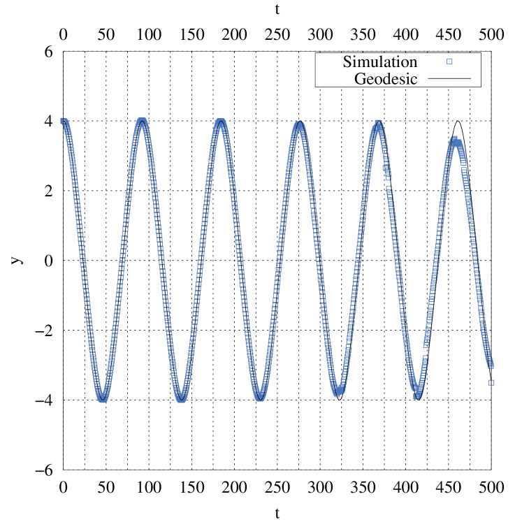
Figure 3: Simulation S1: (a - Upper panel) Maximum density $\rho_{\rm max}$ and maximum pressure $p_{\rm max}$ vs time $t$. The vertical lines highlight the pericenter (purple) and apocenter (green) passages of the corresponding test particle geodesic. (b - Lower panel) Position $(x=0,y)$ of the maximum density $\rho_{\rm max}$ of the cloud and the corresponding test particle geodesic (black) vs time $t$.

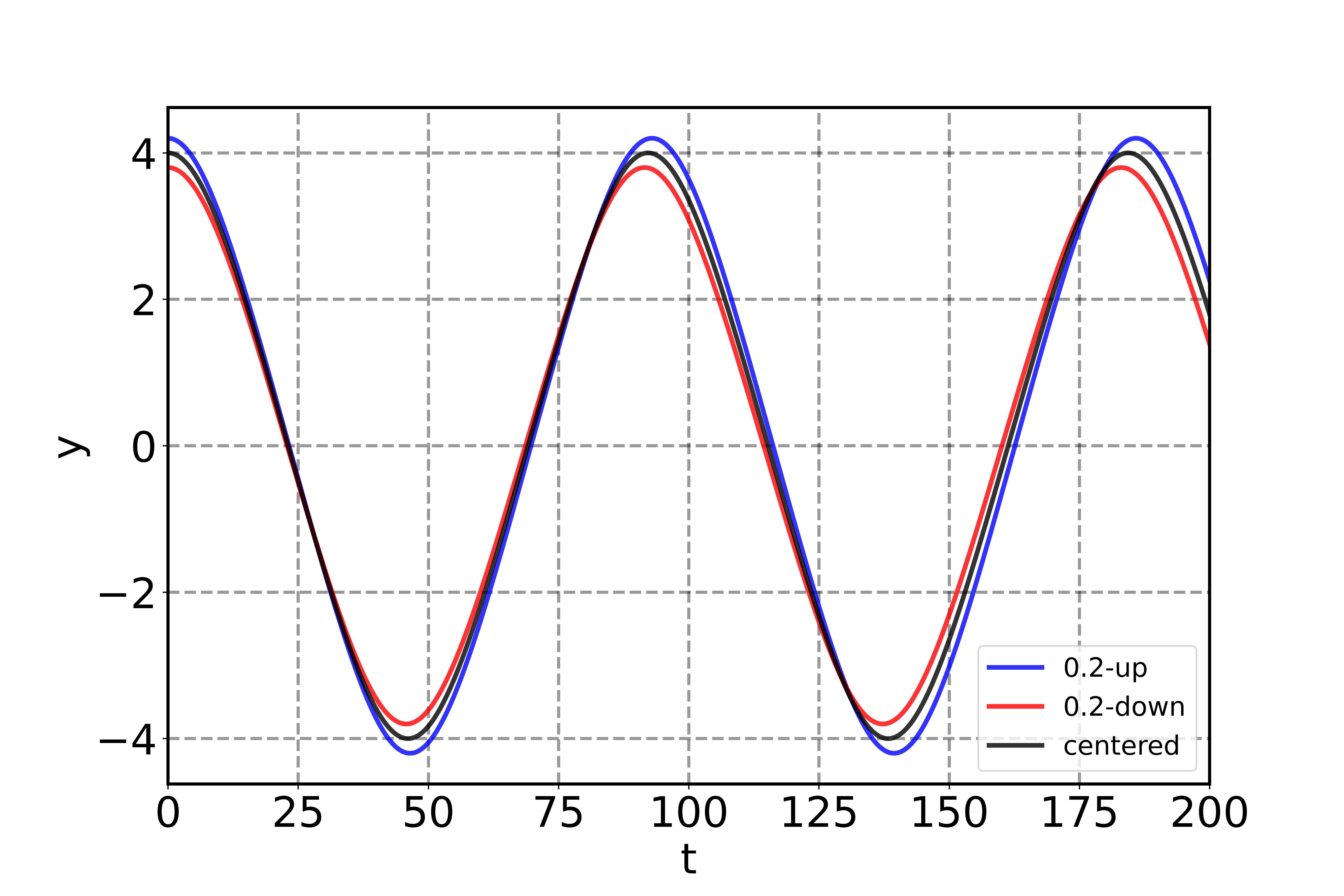
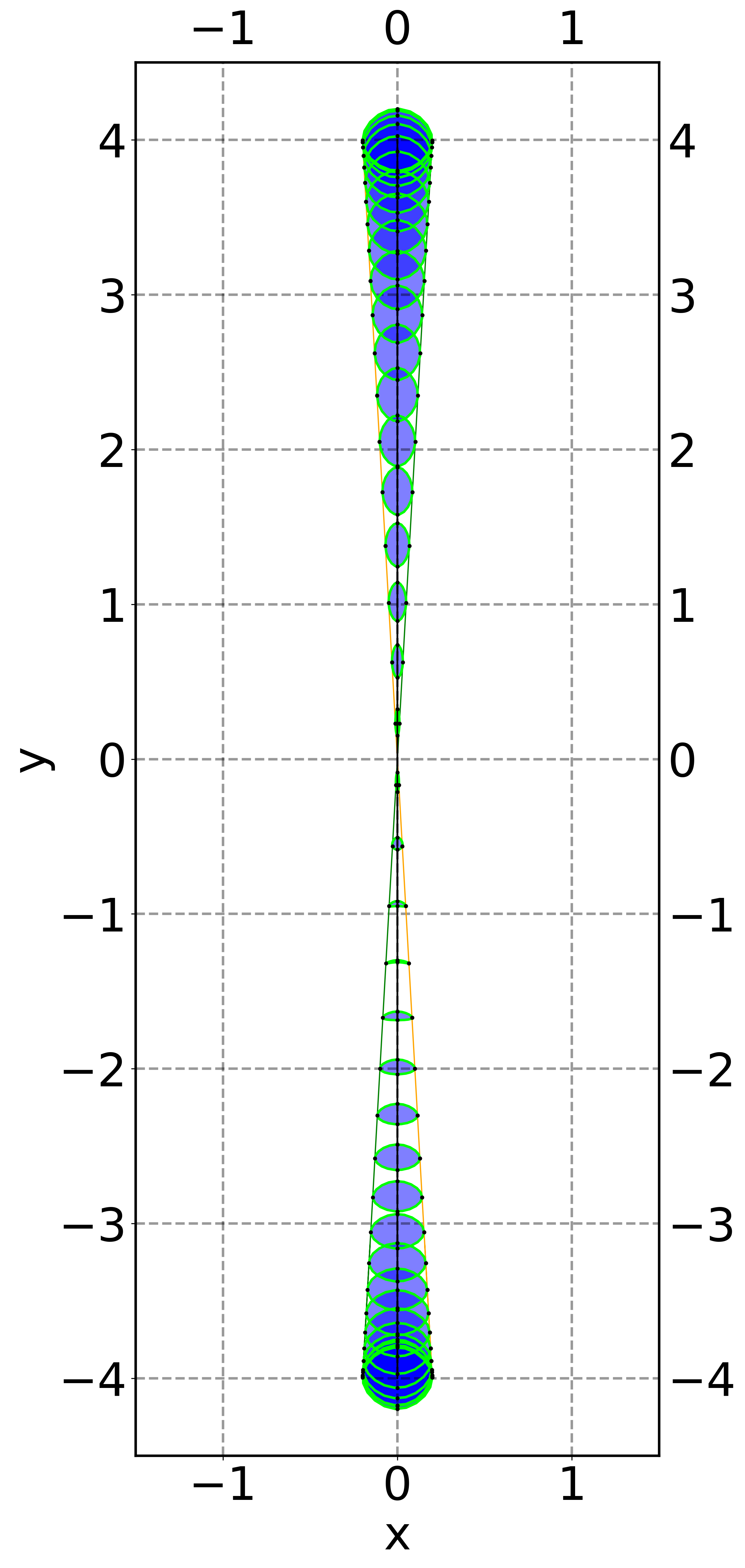
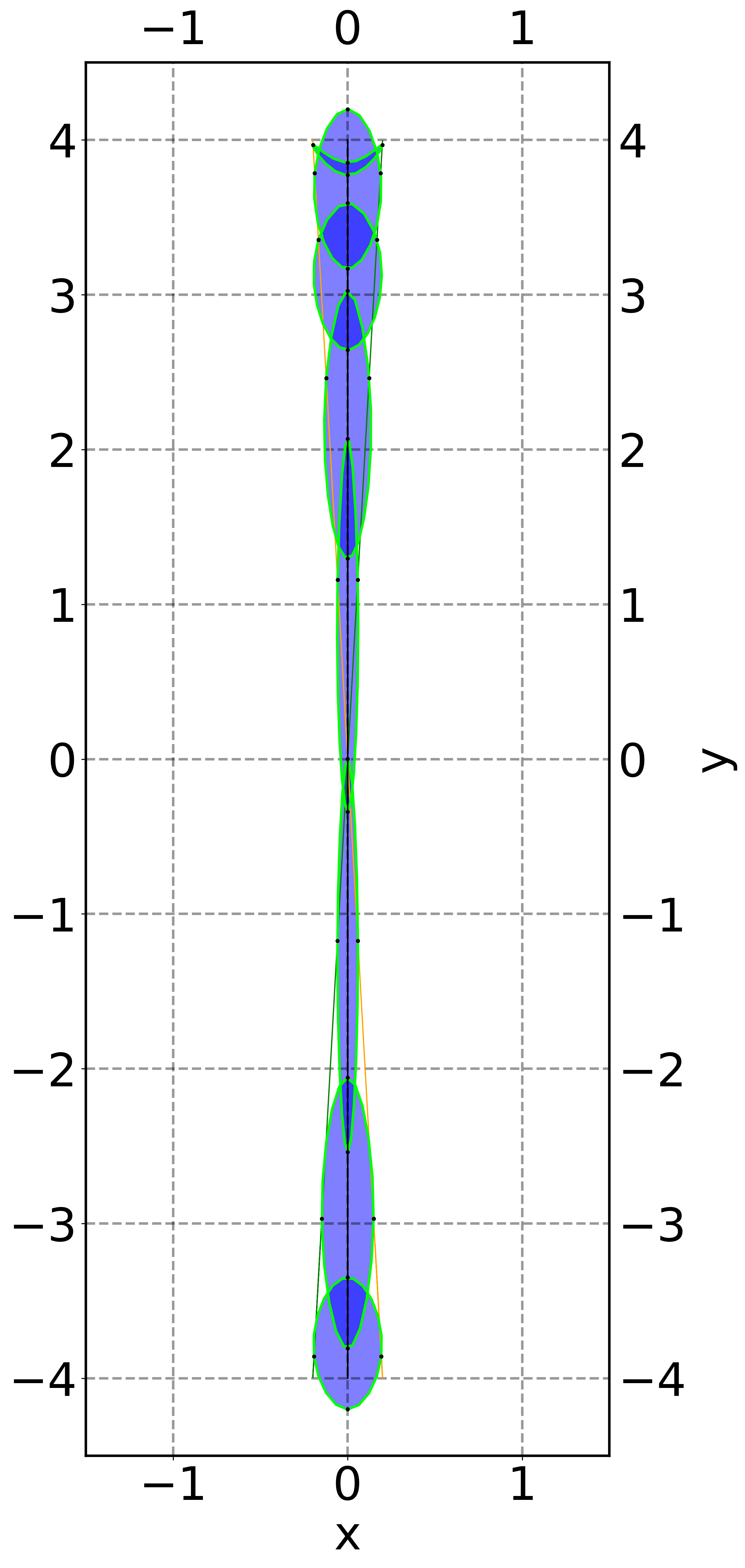
Figure 4: Simulation S1: Comparison with geodesics of surface points of the cloud. (a - Upper panel) Position $(x=0,y)$ of geodesics of upper edge, center and lower edge points vs time $t$. (b,c - Lower panels) Geodesic motion of cloud surface points during the first half period (left) and the last half period (right) of the cloud motion.

IV Small and dense clouds (S1, S2 and S3)

In this section we report the simulations regarding small ($R=0.03$) and dense ($\rho_{0}=1$) clouds nearby the BS, that are centered initially at $r_{0}=4$. The parameter choice for these simulations is aimed at approximating the test particle limit, at least in the beginning of the simulations. Starting slightly inside the radius $R_{\rm BS}$ of the BS, the simulations also represent a rather unique scenario, since analogous phenomena would not be feasible for compact objects endowed with a hard surface or an event horizon.

IV.1 S1 – Head-on collision

In the simulation S1 the cloud starts from rest ($v^{r}=v^{\phi}=0$) with its center located at $(x=0,y=4)$. Being gravitationally accelerated towards the BS center $(x=0,y=0)$, the cloud then passes the center with velocity $v^{r}=0.74$. As predicted by the geodesic motion of a test particle with the same initial conditions as those of the cloud, the gas then decelerates, until it reaches the opposite of its starting position $(x=0,y=-4)$, from where it moves back again towards the BS center. The tracking of the maximum density position, exhibited in Fig. 3(b), shows consistency with the respective geodesic motion throughout the simulation. Although the maximum density position follows the geodesic, it can be seen on the snapshots selected in Fig. 2, that during the motion of the cloud debris is released from it, making the cloud lose its initial shape.

To illustrate the expected tidal effects, we compare in Fig. 4 the geodesics of surface points of the cloud. The upper panel shows the position $(x=0,y)$ of the geodesics of the upper edge point, the center and lower edge point versus time $t$, revealing slight changes in the periods that depend on the relative position. In the lower panels we illustrate the geodesic motion of the points of the cloud surface (taken at the beginning of the run $t=0$) and following them during the first half period (left figure) and the last half period (right figure) of the cloud motion.The deformation of the initially spherical cloud surface indicates the squeezing effects found as a result of our simulations.

Studying now the cloud motion in more detail, we note that the initial acceleration of the cloud is accompanied by a compression transverse to the gas motion, that is related to the medium’s resistance to the motion. The change of the direction of motion together with thermal rebound causes several of such compressions which are dominant until $t=200$. After this point, another type of compression-expansion oscillation takes place. Namely, the now more extended cloud is more susceptible to tidal forces, which are maximal at the BS center and minimal an the orbit’s apocenters. These forces then give rise to compression-expansion cycles endowed with half of the period of the orbit, where maximal compression is found when the cloud passes through the origin (pericenter) and maximal expansion at the apocenters of the orbit. The cloud then continually increases in size at the apocenters, providing feedback to the tidal compression at the center, making the cloud even broader. These self-sustained processes then dismantle the cloud. The cycles can be tracked by following the maximum density and the maximum pressure of the gas, as shown in Fig. 3(a).

Another important debris formation mechanism occurs by the formation of short-term double tails, which lose their shape through gas-tail collision, when the motion of the cloud changes direction. In the collision the gas of the cloud leads to shock waves in the tails, while the tails also create minor shock waves, that travel and bounce inside the cloud. Also, low density debris constantly hits the cloud, since its trajectory does not necessarily follows the geodesic. A combination of these two types of gas-gas interaction then triggers turbulence in the cloud’s tail and surface, extracting chunks of fluid.

The combination of these two mechanisms will eventually destroy the original shape of the cloud as seen in the last snapshot of Fig. 2.

IV.2 S2 – Closed elliptic orbit

Figure 5: Simulation S2: Selected snapshots of the density (with logarithmic color coding) for an elliptic orbit of the gas cloud around the BS.

The second simulation reported here is done by matching the initial conditions of the cloud with those of a test particle on a closed elliptic orbit. It is obtained by giving the gas an angular momentum $\mathbf{L}=1.7890$, while all the other simulation parameters remain the same. A selection of snapshots from S2 is shown in Fig. 5(a) and (b). Once again, the position of the maximum density of the cloud follows the geodesic motion, as can be seen in Fig. 6(b), where the radial distance $r$ and azimuthal angle $\varphi$ of $\rho_{\rm max}$ are shown and compared to the corresponding geodesic motion.

Now the angular motion of the cloud prevents the previous abrupt change of direction in its trajectory. Thus no significant cloud-tail interaction is observed. On the other hand, the rarefied gas (with a density on the order of magnitude of the atmospheric density) that is extracted from the cloud since the beginning of the simulation, falls almost freely towards the BS center. Although not significant for the cloud itself in terms of fluid-loss, such tiny debris is accelerated, reaching high velocities (similar to the ones observed in S1) and, after crossing the BS center it re-encounters the cloud at about $t=50-60$. Although no changes in the course of the cloud center are found as a result of such an encounter, the collision of the outgoing debris and the cloud, which is at that moment traveling towards the center, generate turbulence through a shock wave encounter. Indeed, shock waves formed by rarefied gas fronts moving outward keep hitting the cloud and its tail during the simulation, making the tail and the cloud’s border turbulent.

On the other hand, cycles of compression-expansion are still present. The first peak of the maximum pressure, shown in Fig. 6(a), is related to the initial conditions of the cloud. The start of the motion of the cloud through the atmosphere, which must indeed make its way through the medium, causes the first compression of the gas. This compression then thermally rebounds and starts to oscillate. This mode of oscillation competes with the cycles of expansion-compression similar to the ones found in the second half of the simulation S1. Since the latter increase in amplitude, after $t=200$ these modes dominate the simulation. Indeed, now synchronized with the apo- and pericenters, these cycles become the main reason for the cloud’s deformation. The finale of the simulation, illustrated by the snapshots in Fig. 5(b), shows how the increasing amplitude of these cycles increasingly deforms the broadened and elongated cloud and thus, similarly to S1, turbulence is triggered at its borders and extracts gas.

Figure 6: Simulation S2: (a -Upper panel) Maximum density $\rho_{\rm max}$ and maximum pressure $p_{\rm max}$ vs time $t$. The vertical lines highlight the pericenter (purple) and apocenter (green) passages of the corresponding test particle geodesic. (b - Lower panel) Position $(r,\varphi)$ of the maximum density $\rho_{\rm max}$ (blue) of the cloud and the corresponding test particle geodesic (black) vs time $t$.

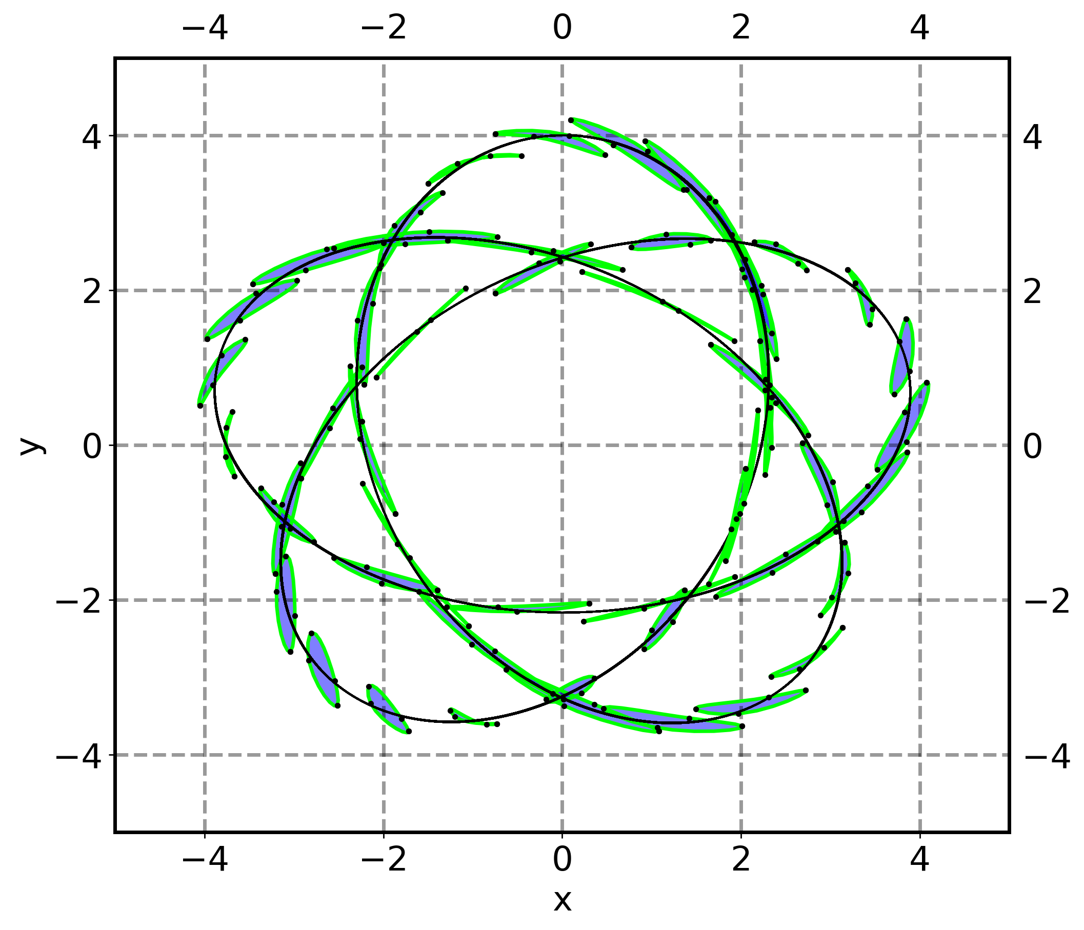
Figure 7: Simulation S2: Comparison with geodesics of surface points of the cloud. (a - Upper panel) Geodesic motion of cloud surface points during the first half of the cloud motion. (b - Lower panel) Geodesic motion of cloud surface points during the second half of the cloud motion.

We illustrate the purely tidal effects, in Fig. 7, where we evolve the geodesics of surface points of the cloud. The upper panel shows the geodesic motion of the points of the cloud surface (taken at the beginning of the run $t=0$) during the first half of the run, while the lower panel illustrates the second half. Again, the deformation of the initially spherical cloud surface due to tidal effects can already be expected from the geodesics deviations. Although significant, these deviations do not take into account hydrodynamic effects that also influence the shape of the cloud.

IV.3 S3 – Circular orbit

Finally, we have performed a third simulation, S3, regarding close-by compact clouds. The angular momentum of the cloud was set to $\mathbf{L}=3.583$ for S3. This angular momentum corresponds to the one of a circular orbit of a test particle at coordinate radius $r=4$ around the BS. A set of selected snapshots for this simulation is shown in Fig. 8. The position of the maximum density $\rho_{\rm max}$ follows again the geodesic motion, as seen in Fig. 9.

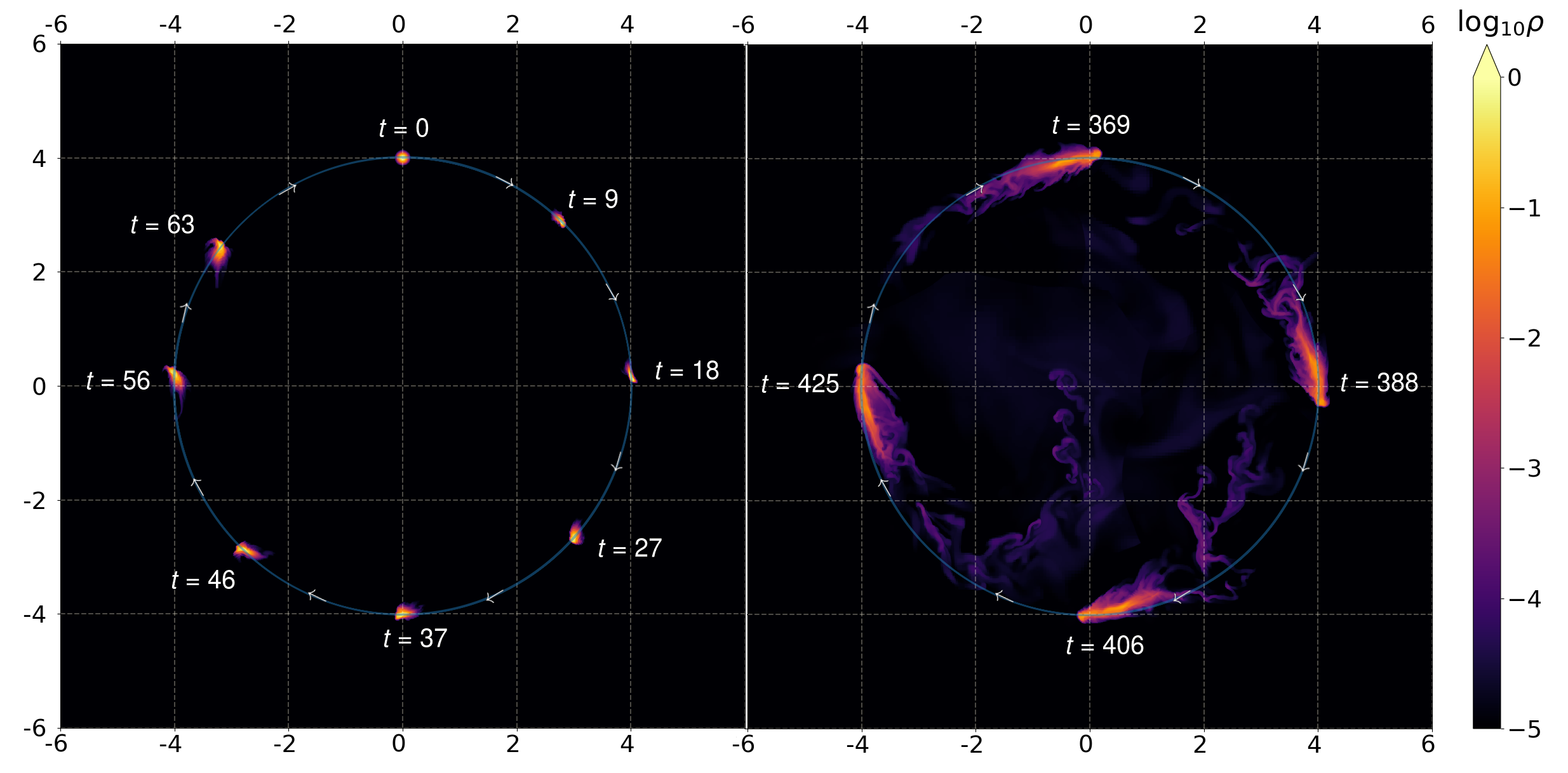
Figure 8: Simulation S3: Selected snapshots of the density (with logarithmic color coding) for a circular orbit of the gas cloud around the BS.

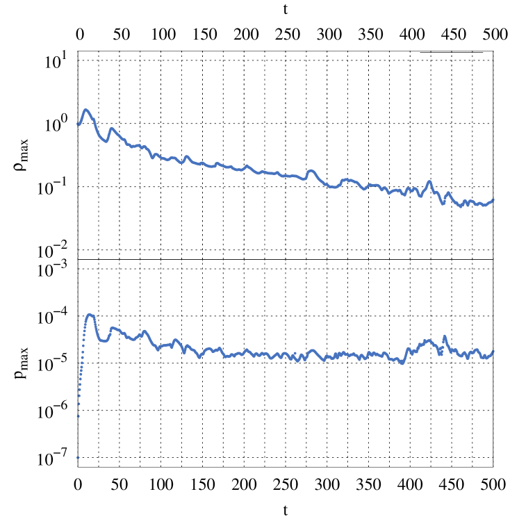
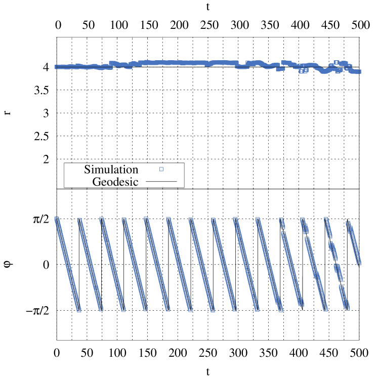
Figure 9: Simulation S3: (a - Upper panel) Maximum density $\rho_{\rm max}$ and maximum pressure $p_{\rm max}$ vs time $t$. (b - Lower panel) Position $(r,\varphi)$ of the maximum density $\rho_{\rm max}$ (blue) of the cloud and the corresponding test particle geodesic (black) vs time $t$.

For circular orbits there are no peri- or apocenters, meaning that the cycles of contraction-expansion of the gas should not be present, since the tidal forces do not change for a constant radius. Indeed, as seen in Fig. 9(a), the maximum density $\rho_{\rm max}$ and the maximum pressure $p_{\rm max}$ do not feature strong periodic oscillations. The first peak of the pressure is due to the initialization of the cloud movement, and the decreasing value of the maximum density is related to the tail formation. Indeed, through the course of the simulation a prominent tail is formed. Tail formation is now mainly related to the cloud movement through the medium, and since the cloud does not suffer transverse expansion, the tail is free to increase in the direction parallel to the gas motion. The elongated tail is then also susceptible to the Kelvin-Helmholtz instability and debris-cloud collisions similar to the ones found in S1 and S2. Thus gas is slowly extracted from the cloud-tail formed structure through turbulence. Cloud-debris collision cannot be prevented in the circular orbit, since rarefied debris generation is also observed for S3.

IV.4 Discussion

Comparing these results with the near-by clouds simulated in [48], it is seen that the different BS model, a rotating mini-BS, employed in [48] and the different initial conditions for the cloud create contrasting gas behavior. Regarding the head-on collision, for a spherically symmetric BS, instead of Lense-Thirring dominated flows as present for rotating BSs, local tidal forces dominate the fluid. For that reason effects such as compression/expansion cycles combined with gas-tail and gas-debris collisions deform the cloud much faster than in the presence of a rotating BS. By giving the cloud angular momentum, such effects become less dramatic, since the trajectory of the fluid in the radial direction becomes less substantial. Indeed, by choosing a circular orbit, only gas-debris collision remains as a gravity caused disruption mechanism. On the other hand, for this circular orbit the gas must be provided with initial angular momentum. Then its movement through a static medium generates a prominent tail.

The debris formation mechanisms discussed in this section are summarized below, and their importance for each simulation is indicated in table 2.

1. Tail-cloud collision - Present when dramatic changes in the direction of motion of the cloud are realized. The cloud’s tail collides directly with the cloud’s main body, eliminating gas from its surface through strong shear forces.

2. Compression-expansion cycles - Present when apocenters and pericenters are encountered in the orbit. The cloud suffers increasingly periodic compression and subsequent expansion cycles, synchronized with the orbit’s extrema. Such cycles deform the cloud, increasing its size and extracting gas from it during the contraction phases.

3. Debris-cloud collision - Present when rarefied gas from the cloud’s surroundings re-encounters the cloud after passage through the BS center. Such collisions trigger turbulence in the cloud’s surface, extracting gas.

Label	Tail-cloud collision	Compression-expansion cycles	Debris-cloud collision
S1	strong	strong	yes
S2	weak	middle	yes
S3	not present	not present	yes

Table 2: Debris formation mechanisms for near-by dense small clouds orbiting the BS.

Based on these three simulations we put forward a conjecture on the lifetime of small dense clouds nearby the compact spherically symmetric BSs. Since for head-on collisions all three debris mechanisms are present, clouds on such trajectories seem to be the least stable ones under the given conditions. Less strong compression and expansion cycles as well as the absence of cloud-tail interaction will provide a longer lifetime for clouds on elliptical orbits. Finally, by eliminating the dramatic changes of the tidal forces on the clouds, circular orbits will be the most stable ones.

V Circular orbits of extended clouds (S4 and S5)

In this section we report simulations of extended gas clouds on (initially) circular orbits around a compact spherically symmetric BS (S4), and compare with the simulations of such clouds around a Schwarzschild BH of the same mass (S5).

V.1 Setup

We have chosen the setup to avoid the expansion-contraction cycles and tail-gas interactions, that arise otherwise as shown in section 4. The angular momentum of test particles on circular orbits is given by

$$\mathbf{L}^{2}=\frac{g_{tt}^{\prime}}{g_{tt}}\Bigg{(}\frac{2}{r_{0}^{3}}-\frac{g_{tt}^{\prime}}{g_{tt}r_{0}^{2}}\Bigg{)}^{-1}.$$ (24)

The initial radial position of the cloud center is chosen to be $r_{0}=10$, a value of the radial coordinate where the metrics of the BS and the corresponding Schwarzschild BH are already very similar, as seen in Fig. 1(b). Therefore the initial angular momentum required for the circular geodesics in these spacetimes is very similar as well, $\mathbf{L}_{\rm BH}-\mathbf{L}_{\rm BS}\approx 10^{-4}$. On the other hand this value of the radial coordinate is not too far from the inner spacetime regions, where the metrics start to differ significantly, representing therefore a meaningful choice for the comparison of the simulations.

The relatively big extension of the cloud, with standard deviation $R=0.3$, is chosen to achieve pressure gradients, that are sufficient to realize considerable tidal effects. These should substantially trigger accretion, but in a manner that the cloud could remain a reservoir of gas during the first stage of the simulation (before complete disruption). To realize the initially circular orbits we have chosen in both simulations an angular momentum of $\mathbf{L}=6.075$ for the entire cloud, as obtained from eq. (24) for $r_{0}=10$.

V.2 Simulations

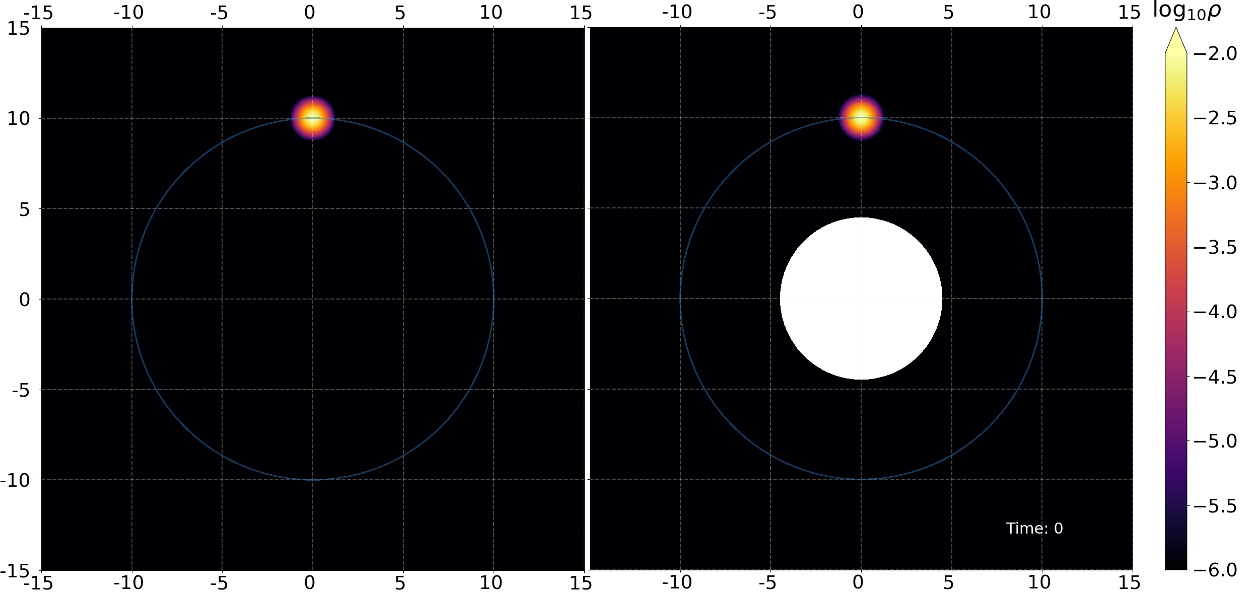
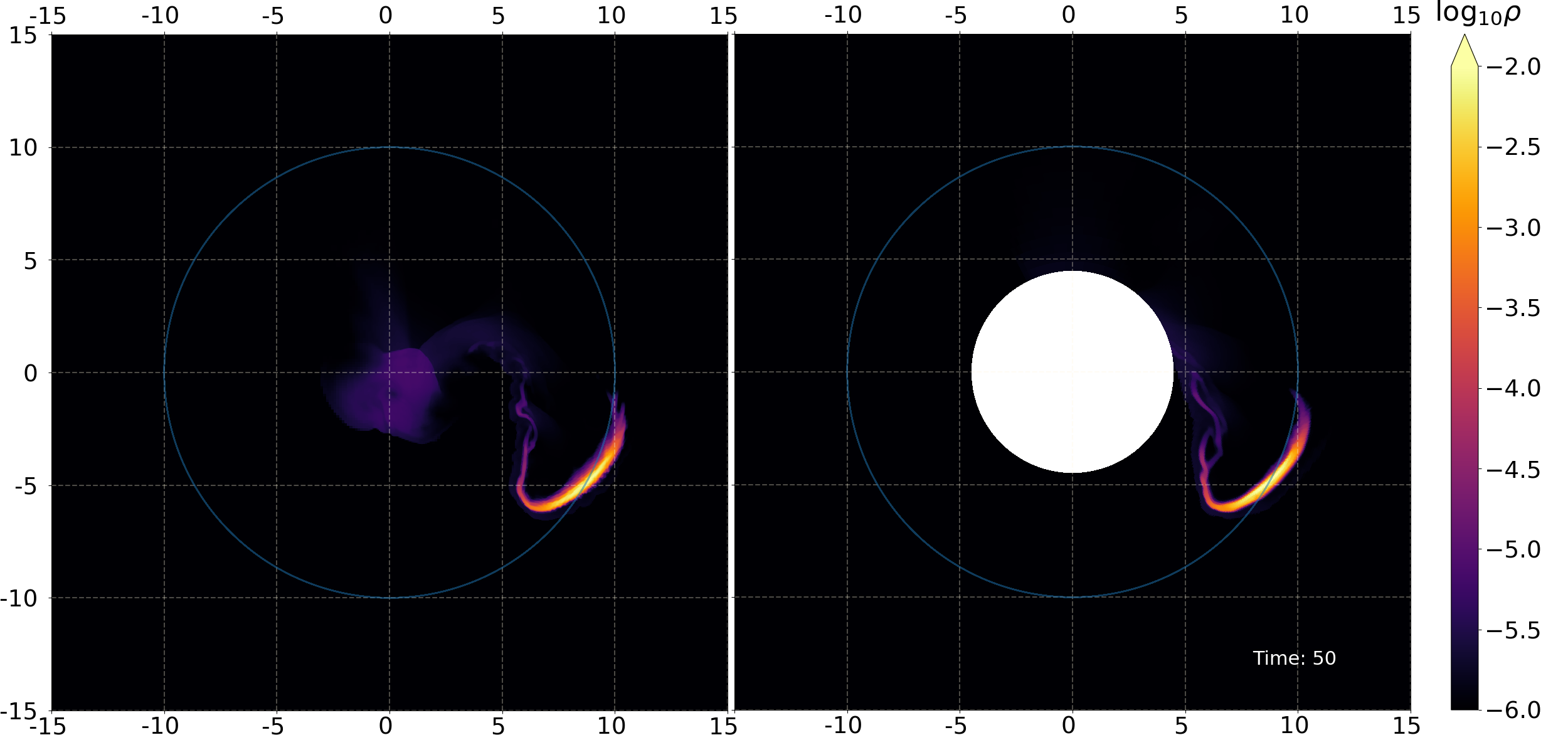
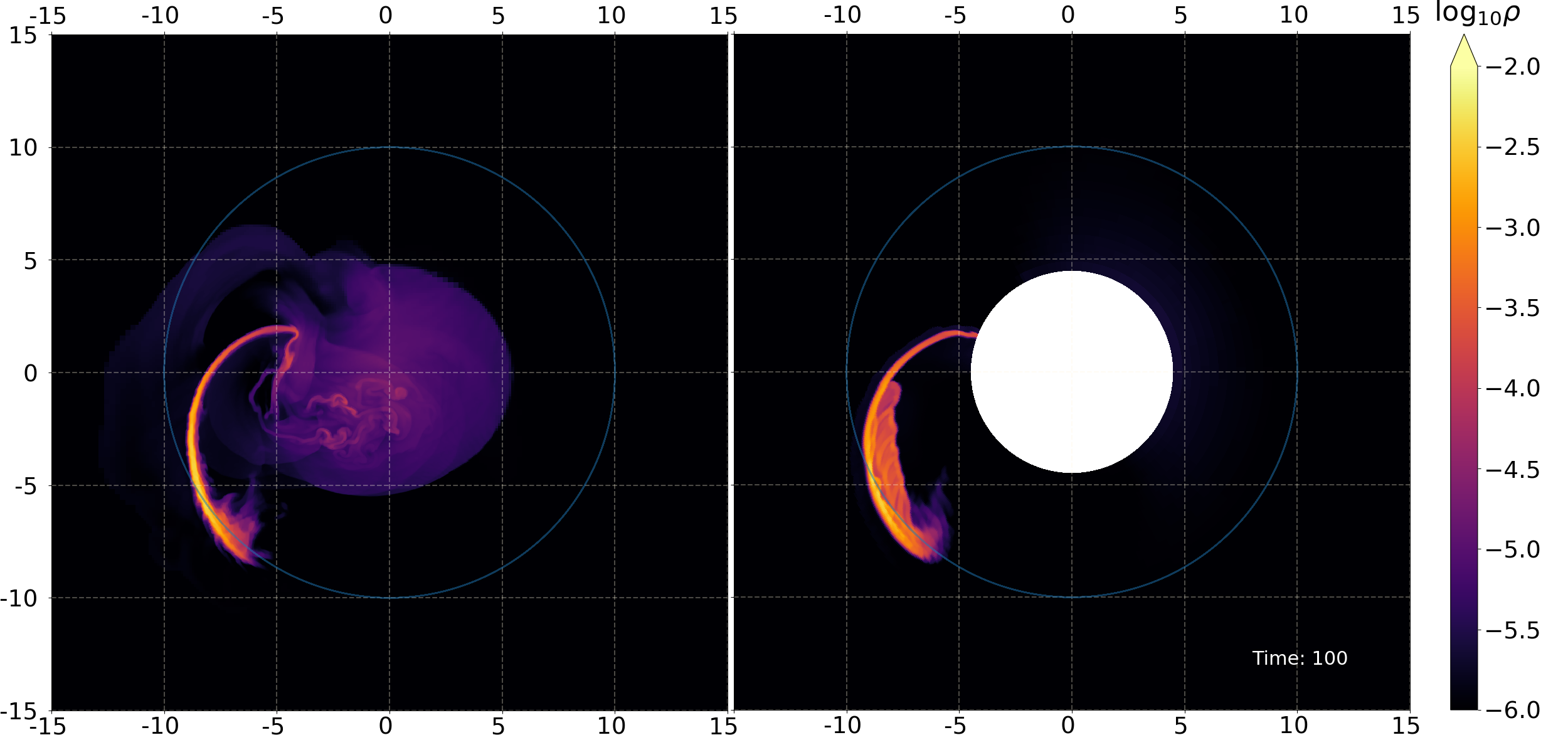
Figure 10: Simulations S4 and S5: Selected snapshots at time $t=0$, $50$ and $100$ of the density (with logarithmic color coding) for an (initially) circular orbit of the gas cloud around the BS (S4, left) and the Schwarzschild BH (S5, right).

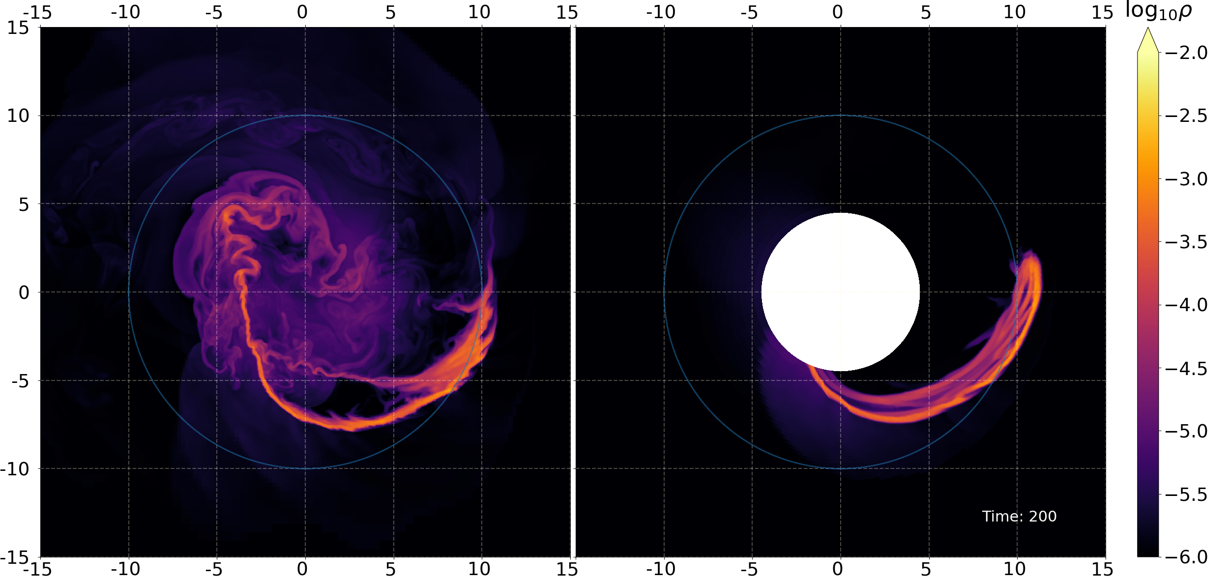
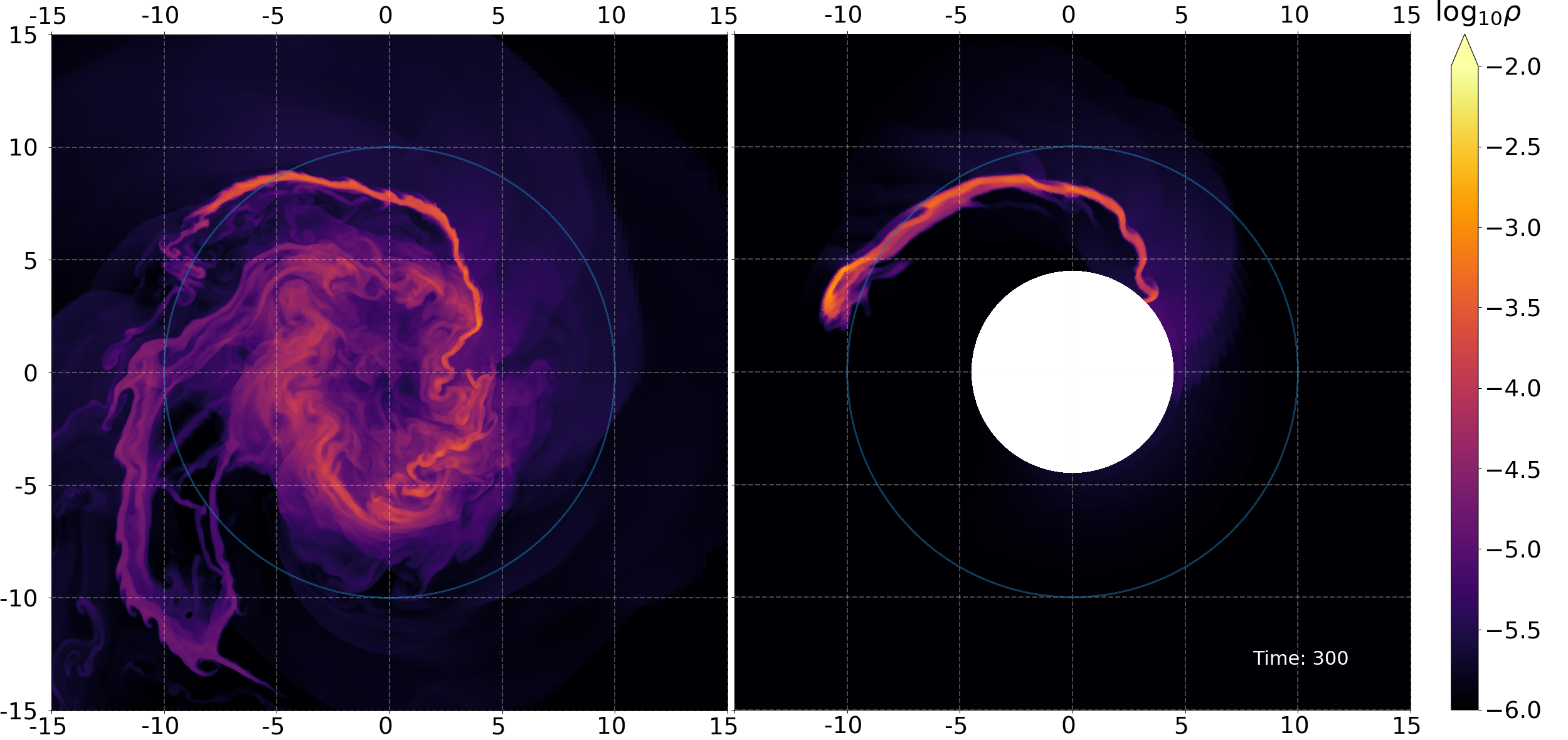
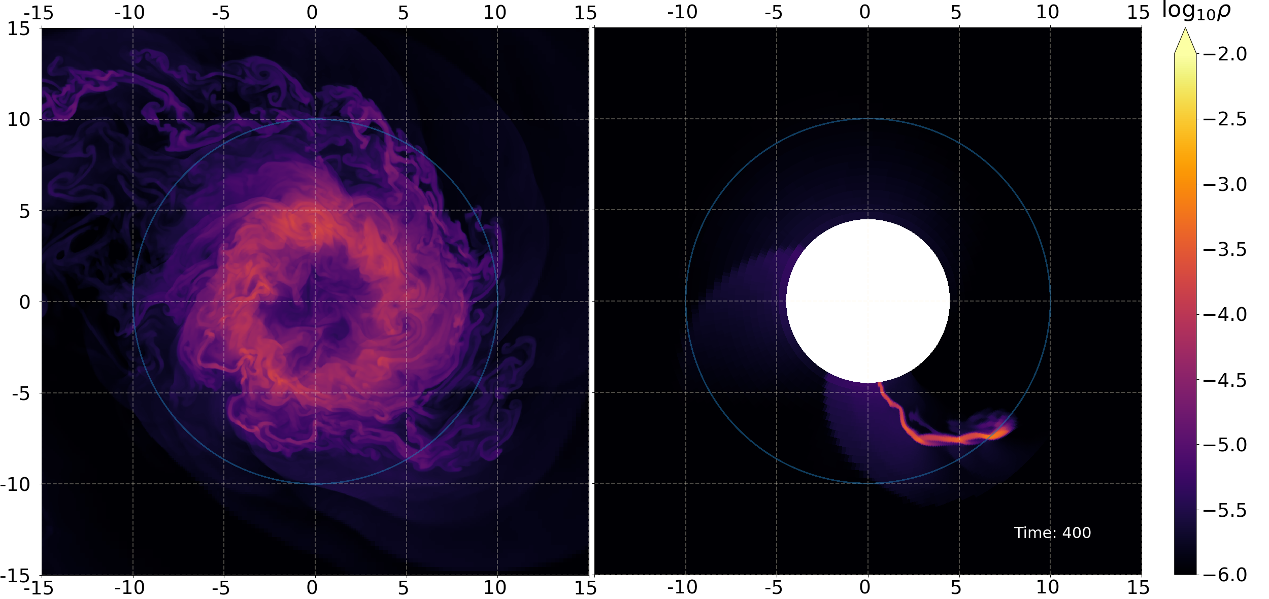
Figure 11: Simulations S4 and S5: Selected snapshots at time $t=200$, $300$ and $400$ of the density (with logarithmic color coding) for an (initially) circular orbit of the gas cloud around the BS (S4, left) and the Schwarzschild BH (S5, right).

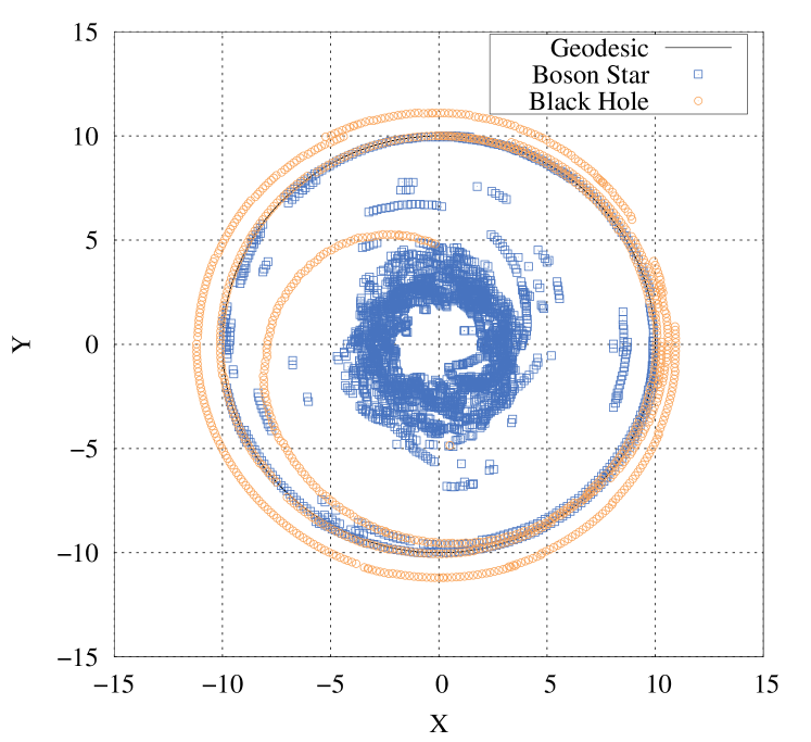
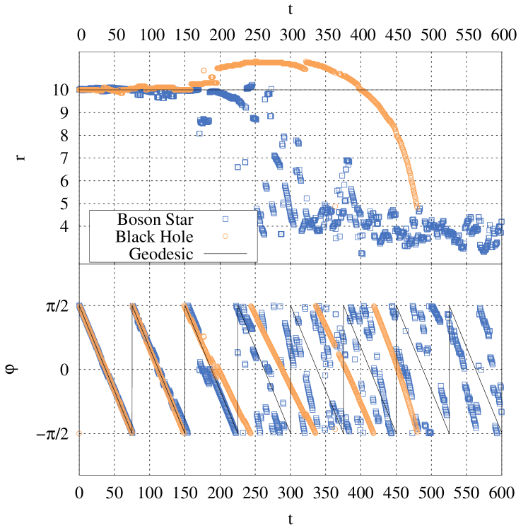
Figure 12: Simulations S4 and S5: Position $(x,y)$ (left) and $(r,\varphi)$ vs time $t$ (right) of the maximum density $\rho_{\rm max}$ of the cloud around the BS (blue) and the Schwarzschild BH (orange) for an (initially) circular orbit, together with the corresponding test particle geodesic (black).

A set of selected snapshots of the gas density, in logarithmic scale, is shown in Fig. 10 and Fig. 11 for the two simulations. They display the initial accumulation of less dense (but high pressure) fluid at the center of the BS. The denser gas is then seen to start forming a turbulent disk-like structure around the BS, where centrifugal forces keep the denser gas from falling towards the BS center. The disk-like structure is well developed for $t=400$, as seen in Fig. 11. This structure seems to become stable and less turbulent towards the end of the simulation. Spiralling shock waves are formed during this process, and keep on going until the end of the simulation. This endphase of the BS simulation S4 contrasts completely with the endphase of the BH simulation S5, where the gas more or less disappears being swallowed by the BH.

Tracking the position of the maximum density for both simulations, as shown in Fig. 12, it is possible to glean insight concerning the general output of the simulations, and their comparison with the test particle orbit. Before $t=150$, which represents approximately the period of the orbit, the maximum density $\rho_{\rm max}$ follows the geodesic in both simulations. For the BS the trajectory then starts to deviate from the circular orbit due to gas-gas interaction and the competition with new dense spots that emerge on the grid. For the BH the gas can be radially stretched freely; and from $t=150$ to $t=400$ the position of the maximum density even exceeds the radius of the circular orbit. At this stage the gravitational attraction finally takes over, pulling the entire cloud towards the event horizon. This happens in such a way that after $t=500$ almost no gas is left on the grid. Indeed such an outcome is expected since for this spacetime the cloud starts partially inside the ISCO of the BH, which is located at the radius $R_{\textrm{ISCO}}=10.5084$.

The BS simulation on the other hand continues beyond this time, since the gas keeps orbiting the center of the BS due to the absence of an event horizon or a hard surface. Therefore we have continued the simulation until $t=1500$.

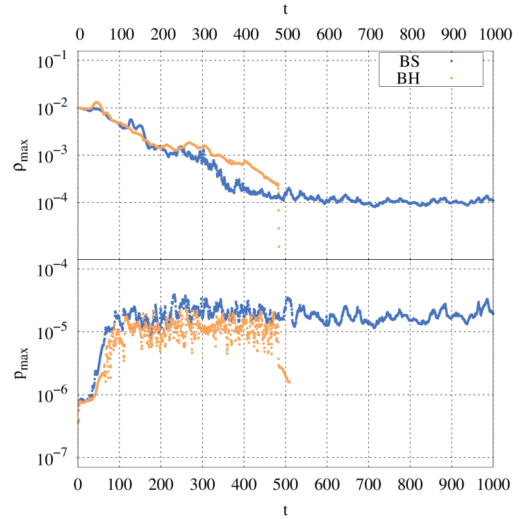
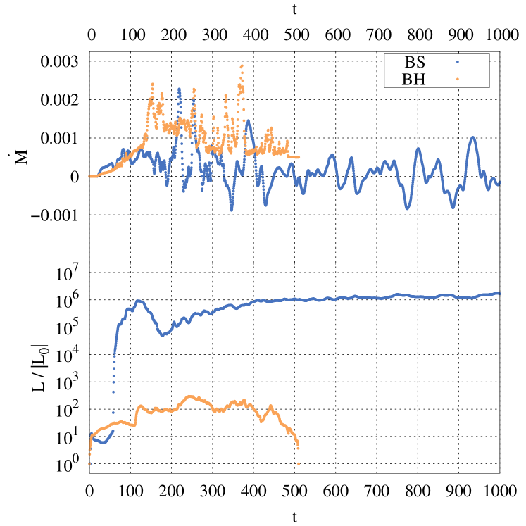
Figure 13: Simulations S4 and S5: (Upper panel) Maximum density $\rho_{\rm max}$ and maximum pressure $p_{\rm max}$ vs time $t$ of the cloud around the BS (blue) and the Schwarzschild BH (orange) for an (initially) circular orbit. (Upper panel) Mass flux $\dot{M}$ and normalized total luminosity $L/L_{0}$ for the BS (blue) and the Schwarzschild BH (orange).

The global variables of interest are shown in Fig. 13. The decrease of the maximum density $\rho_{\rm max}$ is similar for both spacetimes for a long time. Thus after the disruption initiates, which results from the combination of transverse squeezing and spaghettification, the fluid does not get significantly compressed. The maximum density then stabilizes for the BS simulation, indicating the existence of a final steady state of the fluid. Analogously, for both simulations the maximum pressure $p_{\rm max}$ is seen to first increase and then oscillate rapidly, assuming similar values in S4 and S5. However, even though similar in behavior, the nature and the consequences of large pressure values are different for the two spacetimes.

Whereas for the BH spacetime high pressure values remain localized, being only related to the transverse squeezing of the cloud and initial non-vanishing velocities, for the BS spacetime high pressure values reside in a more extended region of the fluid. This region is formed of cloud debris, which floats around the center of the grid. In fact, this region contributes considerably to the total luminosity of the fluid. Already during the first stage of the simulation, around $t=70$, the first debris of the cloud reaches the center of the BS and the high pressure region is formed.

This region, although initially not very dense, but featuring high velocities (up to $v^{r}=0.84$), then generates a peak in the total luminosity around $t=120$. This is seen in Fig. 13(b), where besides the maximum density and pressure also the luminosity $L$ (normalized to its initial value $L_{0}$) is shown together with the mass flux $\dot{M}$. After $t=400$ the value of the luminosity from the first peak is again restored, staying almost constant now due to the, now denser, high-pressure region. This constant total luminosity is four orders of magnitude bigger than the highest luminosity found in the BH simulation.

Regarding the mass flux $\dot{M}$, as expected, only positive values of $\dot{M}$ arise in the BH simulation, since it represents the accretion rate in this spacetime. In contrast, in the BS simulation $\dot{M}$ has also negative values. This does, however, not imply the existence of outflows.

V.3 Aftermath

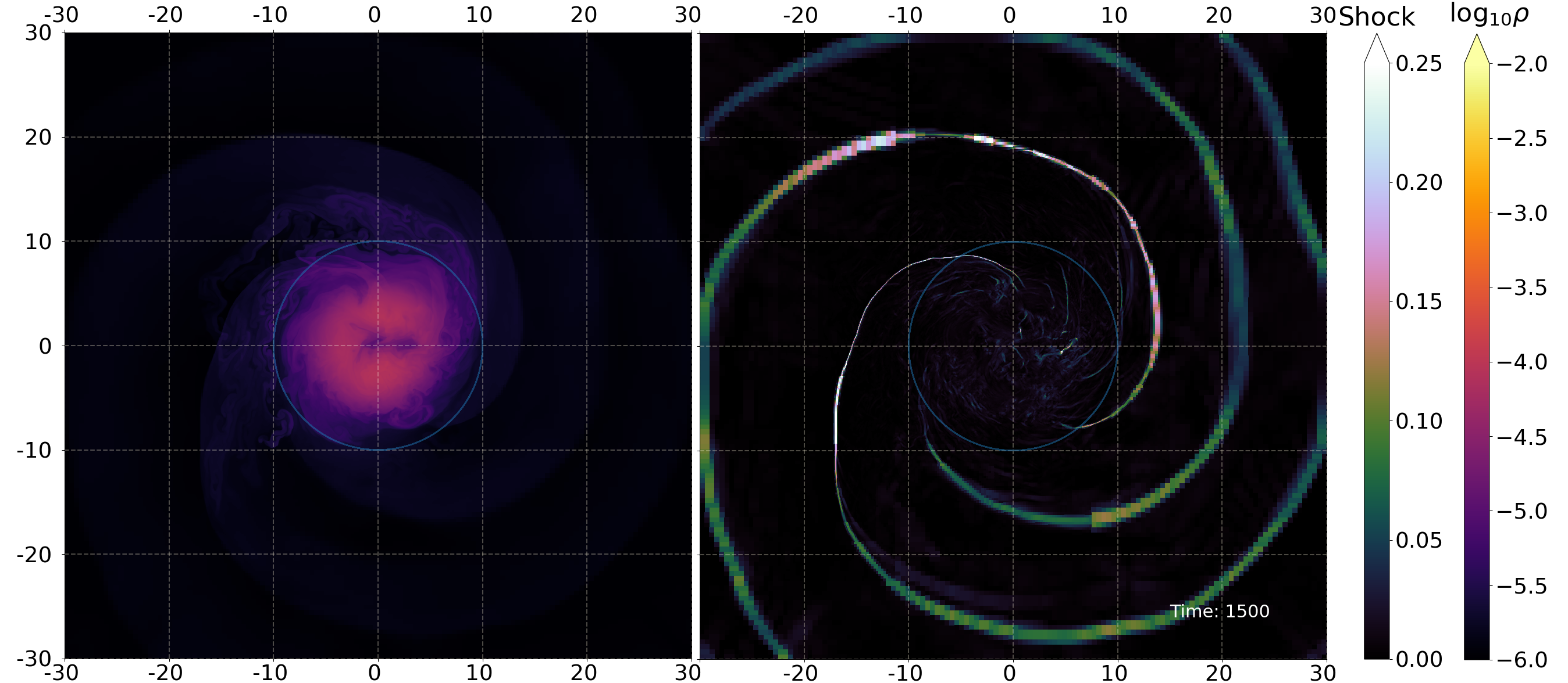
Figure 14: Simulation S4 aftermath at time $t=1500$: Snapshot of the density (with logarithmic color coding) for an (initially) circular orbit of the gas cloud around the BS (left), and snapshot of the shock detector variable (right).

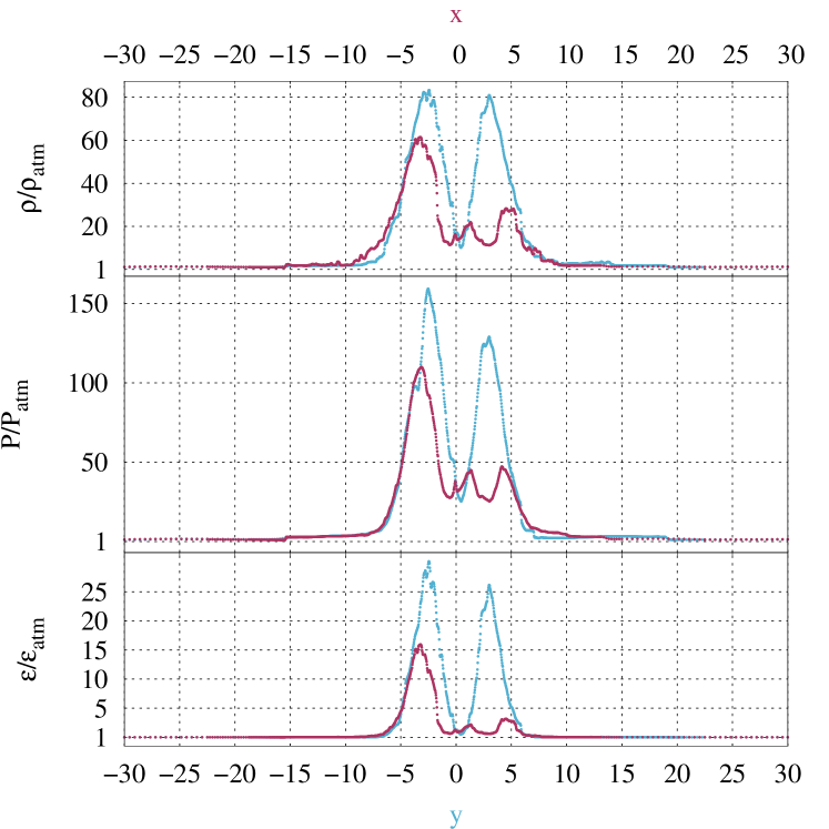
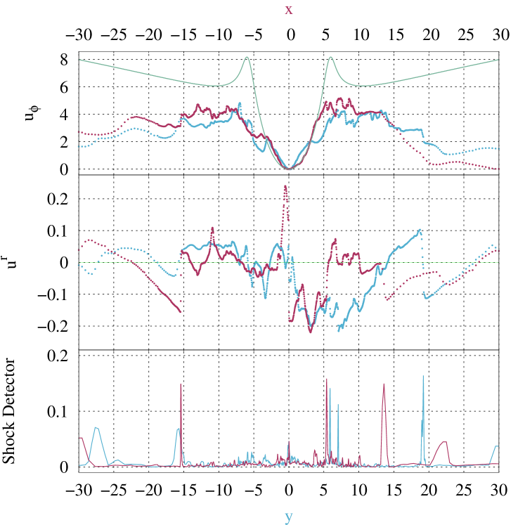
Figure 15: Simulation S4 aftermath at time $t=1500$: (a - Upper panel) Density profile $\rho/\rho_{\rm atm}$, pressure profile $p/p_{\rm atm}$, and emissivity profile $\varepsilon/\varepsilon_{\rm atm}$ along the $x$-axis (red) and the $y$-axis (blue), normalized with respect to the atmosphere values. (b - Lower panel) Angular momentum profile $u_{\varphi}$, radial velocity profile $u^{r}$, and shock detector profile along the $x$-axis (red) and the $y$-axis (blue). Also shown are the Keplerian profiles for $u_{\varphi}$ and $u^{r}$ (green).

Turning now to the aftermath of the simulations, we recall that in the BS simulation a disk-like structure has formed, featuring spiralling shock waves. An example of these waves together with the final density configuration of the gas is shown in Fig. 14, representing the final outcome of the simulation S4.

In order to explore the structure and formation of the shock pattern let us consider slices of the grid along the $x$- and $y$-axis at $t=1500$, the final time-step of the simulation S4. These slices are shown in Fig. 15(a) for the density profile $\rho/\rho_{\rm atm}$, the pressure profile $p/p_{\rm atm}$, and emissivity profile $\varepsilon/\varepsilon_{\rm atm}$, normalized by the respective atmospheric values, and in Fig. 15(b) for the angular momentum profile $u_{\varphi}$, the radial velocity profile $u^{r}$, and the shock detector profile, always for the $x$-axis (red) and the $y$-axis (blue).

In Fig. 15(a) we observe almost symmetric configurations for the density, the pressure and the emissivity along the $y$-axis with respect to the BS center. In contrast, along the $x$-axis the configurations do not exhibit such a symmetry. Whereas the locations of the peaks in $x$ agree with those in $y$ for negative $x$, we observe much lower values for positive $x$ than for negative $x$ for these quantities. Thus we find a residual low density region on its way towards the center of the grid. While this shows how dynamical the aftermath structure is, the balance of centrifugal and gravitational forces keeps a ring-like structure roughly in place, centered at a radial coordinate $2.9\pm 0.2$ (i.e., $2.9$ is the average of the radial coordinates of the maxima of the density, pressure and emissivity profiles at $t=1500$, and $\pm 0.2$ represents their variation). By averaging the values of the angular momentum of the cells in the region $2.9-0.2<r<2.9+0.2$ we obtain $\bar{L}=\bar{u}_{\varphi}=2$. Defining the effective potential $V_{\rm eff}$ of a massive test particle via

$$V_{\rm eff}=-g_{tt}\left(1+\frac{L^{2}}{r^{2}}\right)$$ (25)

we now consider circular geodesics, for which ${V^{\prime}}_{\rm eff}=0$. The circular geodesic with angular momentum $\bar{L}=\bar{u}_{\varphi}=2$ then resides at radial coordinate $r=3.1$, i.e., in the direct vicinity of the ring-like structure. Thus the center of the ring-like structure roughly follows a Keplerian geodesic. The associated effective potential $V_{\rm eff}$ for a test particle with angular momentum $L=2$ is depicted in Fig. 16.

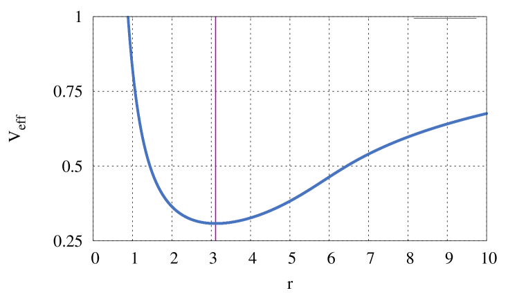
Figure 16: Effective potential $V_{\rm eff}$ for a massive test particle with angular momentum $L=2$. The purple line at $r=3.1$ marks the position of the circular orbit.

The shock structure spiralling outwards accompanying the ring can be understood better with the help of Fig. 15(b). Here we see that the angular momentum distribution of the gas also appears to be symmetric. Note, that besides the data we here also provide the Keplerian angular momenta from eq. (24) (green). The gas motion is then, as expected, not geodesic. The gas has super-Keplerian angular momentum near the center of the grid, but becomes sub-Keplerian outside the radius of the ring. The $u^{r}$ velocities, although small, on the other hand are not symmetric and feature positive and negative values. This reveals how the balance of accreting and out-flowing gas is working.

Interestingly, by comparing these profiles with the shock detector it is possible to infer the origin of the shocks. The positions of the shocks outside the ring coincide with the positions where the radial velocities change abruptly. Indeed, the shocks are formed by the colliding gas moving outwards (due to the centrifugal forces) with the gas moving inwards (due to the gravitational pull). The shocks then have a radial nature, but are dragged along with the rotating gas creating the spiral structure. When the dragged gas gets far from the BS center, it starts being pulled back towards the center, until it reaches another shock wave. Although these collisions do not generate radial velocities strong enough to destroy the ring, they keep generating the shock waves. Due to the nature of the shocks, a meaningful amount of shear is intrinsic to them. Thus this structure is susceptible to cease when viscous time-scales are reached. Nevertheless, due to the highly dynamical scenario this consideration might depend on the nature of the viscosity.

We note that, by the end of the simulation S4, enough gas from the cloud and its surroundings has been spread to the entire grid in a manner that no atmosphere is left. Therefore the shock waves do not represent an artefact of the atmospheric treatment. We also note that the temperature of the gas increases substantially after the disruption, indicating the possibility of ionization. It is possible to infer then that the disk formed would become hot plasma, for which then magnetic fields would be important.

In order to address the fate of the disk-like structure, viscous effects would need to be taken into account. Also, depending on the BS model, accumulation of gas at the BS center from accreting matter of the disk might occur [49].

In closing let us mention that we have also performed another simulation, employing the same parameters as for simulation S4, but with vanishing initial angular momentum. In this case, although very strong radial shock waves are found during the first collision of the gas with the BS, after a time of $t=600$ only minor shock waves are formed, indicating that the rotation of the gas plays an important role in the shock wave dynamics. Because of the large extent of the cloud and the high velocities involved in such a scenario, the fluid oscillation around the BS center becomes rapidly turbulent, and the cloud’s shape is quickly lost. In the aftermath, apart from small vortices generated during the first collisions, the gas resides symmetrically around the BS with a single peak of maximum density and pressure. This highly symmetric configuration is reached after $t=600$.

VI Conclusions

In this paper we have reported simulations regarding the motion and evolution of gas clouds around compact spherically symmetric BSs. We have compared with the motion of particles on geodesics, and have investigated the tidal and hydrodynamic effects on the evolution and final disruption of these clouds. In fact, effects like debris formation and disruption have the tendency to divert the cloud’s gas from corresponding particle geodesic motion. In particular, we have considered two different regimes. The first regime is the one of dense gas spots nearby the BSs.

These nearby clouds feature different debris formation mechanisms, depending on the initial angular momentum provided to them. Namely, the more elliptical the cloud’s initial orbit, the stronger is the debris formation and the observed subsequent disruption, for these effects are more significant when the cloud is susceptible to radial motion. Although the cloud’s center is inclined to follow the particle geodesic motion, these effects tend to deform the clouds’ initial shape and divert portions of the gas from the initial orbit. Particularly for the case in which these small clouds are set out to travel at a constant radius the tidal forces are less significant. On the other hand, the fluid motion through the medium gives rise to a prominent turbulent tail. This turbulence is related to the fact that debris-cloud collisions are still observed. We conclude from the performed simulations that small clouds nearby spherically symmetric BSs are less stable and thus possess a shorter lifetime than the ones in the vicinity of rotating BSs, studied in [48].

In a second regime we have provided simulations aimed at a comparison between extended clouds in a BS spacetime and a Schwarzschild BH spacetime, with both compact objects possessing the same mass. Due to their extension, tidal forces rapidly divert portions of the cloud from their initial orbit, enabling the gas to reach the vicinity of the central objects. Initially in a circular orbit, the clouds are seen to behave in a similar manner in the initial phase of the simulations. But soon important differences arise. Most importantly, due to the absence of an event horizon in the BS simulation, the debris of the cloud does not disappear when accreted. Therefore thermal Bremsstrahlung emissivity is considerably higher and lasts much longer in a BS spacetime. In contrast, in a BH spacetime the gas of the cloud in a close-by circular orbit is totally swallowed by the BH. The absence of an event horizon or a hard surface provides an appropriate environment for the gas to stabilize in a ring-like structure with a spiralling shock wave pattern. In contrast, for a BH spacetime no such structure is formed. We believe that a further analysis of these structures regarding their possible similarities with accretion disk models as well as the effects of viscosity on them is an appealing field for future work.

Here we have selected a stable BS with high compactness in order to be rather close to the BH limit in the simulations. However, most BS solutions of the model feature lower compactness, as seen in Fig. 1. When we choose a less compact BS on the stable branch, but retain comparable conditions for the initial properties of the cloud, we observe qualitatively similar outcomes, as indicated by preliminary simulations. In particular, we retain the formation of a ring-like structure in the aftermath, whose center follows roughly a Keplerian orbit.

In this work we have also provided a preliminary analysis regarding tidal disruption events around compact spherically symmetric BSs. Indeed, such spacetimes turn out to be appealing scenarios for interesting fluid dynamics-related events to arise. Inspired by these first simulations, as future work we shall aim to perform further simulations for different types of BSs, as well as for other exotic compact objects. In particular, regarding rotating spacetimes, we think that performing fully 3D simulations, as well as including magnetic-fields and accretion disks would be fruitful.

References

- [1] B. P. Abbott et al. [LIGO Scientific and Virgo], Phys. Rev. Lett. 116, no.6, 061102 (2016)
- [2] B. P. Abbott et al. [LIGO Scientific and Virgo], Phys. Rev. Lett. 116, no.24, 241103 (2016)
- [3] B. P. Abbott et al. [LIGO Scientific and VIRGO], Phys. Rev. Lett. 118, no.22, 221101 (2017) [erratum: Phys. Rev. Lett. 121, no.12, 129901 (2018)] [arXiv:1706.01812 [gr-qc]].
- [4] K. Akiyama et al. (Event Horizon Telescope) Astrophys. J. 875 L1 (2019)
- [5] K. Akiyama et al. (Event Horizon Telescope) Astrophys. J. Lett. 875 L2 (2019)
- [6] K. Akiyama et al. (Event Horizon Telescope) Astrophys. J. Lett. 875 L3 (2019)
- [7] K. Akiyama et al. (Event Horizon Telescope) Astrophys. J. Lett. 875 L4 (2019)
- [8] K. Akiyama et al. (Event Horizon Telescope) Astrophys. J. Lett. 875 L5 (2019)
- [9] K. Akiyama et al. (Event Horizon Telescope) Astrophys. J. Lett. 875 L6 (2019)
- [10] A. M. Ghez, B. L. Klein, M. Morris and E. E. Becklin, Astrophys. J. 509, 678-686 (1998)
- [11] A. M. Ghez, S. Salim, S. D. Hornstein, A. Tanner, M. Morris, E. E. Becklin and G. Duchene, Astrophys. J. 620, 744-757 (2005) doi:10.1086/427175 [arXiv:astro-ph/0306130 [astro-ph]].
- [12] R. Genzel, R. Schodel, T. Ott, A. Eckart, T. Alexander, F. Lacombe, D. Rouan and B. Aschenbach, Nature 425, 934-937 (2003)
- [13] A. M. Ghez, S. Salim, N. N. Weinberg, J. R. Lu, T. Do, J. K. Dunn, K. Matthews, M. Morris, S. Yelda and E. E. Becklin, et al. Astrophys. J. 689, 1044-1062 (2008)
- [14] S. Gillessen, F. Eisenhauer, S. Trippe, T. Alexander, R. Genzel, F. Martins and T. Ott, Astrophys. J. 692, 1075-1109 (2009)
- [15] R. Genzel, F. Eisenhauer and S. Gillessen, Rev. Mod. Phys. 82, 3121-3195 (2010)
- [16] A. Eckart, A. Hüttemann, C. Kiefer, S. Britzen, M. Zajaček, C. Lämmerzahl, M. Stöckler, M. Valencia-S, V. Karas and M. García-Marín, Found. Phys. 47, no.5, 553-624 (2017)
- [17] V. Cardoso, E. Franzin and P. Pani, Phys. Rev. Lett. 116, no.17, 171101 (2016) [erratum: Phys. Rev. Lett. 117, no.8, 089902 (2016)] [arXiv:1602.07309 [gr-qc]].
- [18] V. Cardoso, S. Hopper, C. F. B. Macedo, C. Palenzuela and P. Pani, Phys. Rev. D 94, no.8, 084031 (2016) [arXiv:1608.08637 [gr-qc]].
- [19] D. A. Feinblum and W. A. McKinley, Phys. Rev. 168, no. 5, 1445 (1968).
- [20] D. J. Kaup, Phys. Rev. 172, 1331 (1968).
- [21] R. Ruffini and S. Bonazzola, Phys. Rev. 187, 1767 (1969).
- [22] D. F. Torres, S. Capozziello and G. Lambiase, Phys. Rev. D 62, 104012 (2000) [astro-ph/0004064].
- [23] E. Berti and V. Cardoso, Int. J. Mod. Phys. D 15, 2209 (2006) [gr-qc/0605101].
- [24] F. H. Vincent, Z. Meliani, P. Grandclement, E. Gourgoulhon and O. Straub, Class. Quant. Grav. 33, no. 10, 105015 (2016) [arXiv:1510.04170 [gr-qc]].
- [25] P. Jetzer and J. J. van der Bij, Phys. Lett. B 227, 341 (1989).
- [26] Y. Kobayashi, M. Kasai and T. Futamase, Phys. Rev. D 50, 7721 (1994).
- [27] E. W. Mielke and F. E. Schunck, In Pronin, P. (ed.): Sardanashvili, G. (ed.): Gravity, particles, and space-time, 391 (1996).
- [28] S. Yoshida and Y. Eriguchi, Phys. Rev. D 56, 762 (1997).
- [29] R. Friedberg, T. D. Lee and Y. Pang, Phys. Rev. D 35, 3658 (1987). doi:10.1103/PhysRevD.35.3658
- [30] F. D. Ryan, Phys. Rev. D 55, 6081 (1997).
- [31] F. E. Schunck and E. W. Mielke, Phys. Lett. A 249, 389 (1998).
- [32] F. E. Schunck and E. W. Mielke, Gen. Rel. Grav. 31, 787 (1999).
- [33] B. Kleihaus, J. Kunz and M. List, Phys. Rev. D 72, 064002 (2005) [gr-qc/0505143].
- [34] B. Kleihaus, J. Kunz, M. List and I. Schaffer, Phys. Rev. D 77, 064025 (2008) [arXiv:0712.3742 [gr-qc]].
- [35] A. Bernal, J. Barranco, D. Alic and C. Palenzuela, Phys. Rev. D 81, 044031 (2010) [arXiv:0908.2435 [gr-qc]].
- [36] B. Hartmann, B. Kleihaus, J. Kunz and M. List, Phys. Rev. D 82, 084022 (2010) [arXiv:1008.3137 [gr-qc]].
- [37] B. Kleihaus, J. Kunz and S. Schneider, Phys. Rev. D 85, 024045 (2012) [arXiv:1109.5858 [gr-qc]].
- [38] L. G. Collodel, B. Kleihaus and J. Kunz, Phys. Rev. D 99, no. 10, 104076 (2019) [arXiv:1901.11522 [gr-qc]].
- [39] H. B. Li, S. Sun, T. T. Hu, Y. Song and Y. Q. Wang, Phys. Rev. D 101, no. 4, 044017 (2020) [arXiv:1906.00420 [gr-qc]].
- [40] V. Diemer, K. Eilers, B. Hartmann, I. Schaffer and C. Toma, Phys. Rev. D 88, 044025 (2013) [arXiv:1304.5646 [gr-qc]].
- [41] C. F. B. Macedo, P. Pani, V. Cardoso and L. C. B. Crispino, Phys. Rev. D 88, no.6, 064046 (2013) [arXiv:1307.4812 [gr-qc]].
- [42] P. Grandclément, C. Somé and E. Gourgoulhon, Phys. Rev. D 90, 024068 (2014) [arXiv:1405.4837 [gr-qc]].
- [43] Z. Meliani, F. H. Vincent, P. Grandclement, E. Gourgoulhon, R. Monceau-Baroux and O. Straub, Class. Quant. Grav. 32, no. 23, 235022 (2015) [arXiv:1510.04191 [astro-ph.HE]].
- [44] P. Grandclément, Phys. Rev. D 95, 084011 (2017) [arXiv:1612.07507 [gr-qc]].
- [45] M. Grould, Z. Meliani, F. H. Vincent, P. Grandclément and E. Gourgoulhon, Class. Quant. Grav. 34, 215007 (2017) [arXiv:1709.05938 [astro-ph.HE]].
- [46] L. G. Collodel, B. Kleihaus and J. Kunz, Phys. Rev. Lett. 120, no. 20, 201103 (2018) [arXiv:1711.05191 [gr-qc]].
- [47] M. C. Teodoro, L. G. Collodel and J. Kunz, [arXiv:2011.10288 [gr-qc]].
- [48] Z. Meliani, F. Casse, P. Grandclément, E. Gourgoulhon and F. Dauvergne, Class. Quant. Grav. 34, no. 22, 225003 (2017).
- [49] H. Olivares, Z. Younsi, C. M. Fromm, M. De Laurentis, O. Porth, Y. Mizuno, H. Falcke, M. Kramer and L. Rezzolla, Mon. Not. Roy. Astron. Soc. 497 (2020) no.1, 521-535 [arXiv:1809.08682 [gr-qc]].
- [50] E. Seidel and W. M. Suen, Phys. Rev. Lett. 72 (1994) 2516 [arXiv:gr-qc/9309015 [gr-qc]].
- [51] N. Sanchis-Gual, F. Di Giovanni, M. Zilhão, C. Herdeiro, P. Cerdá-Durán, J. A. Font and E. Radu, Phys. Rev. Lett. 123 (2019) no.22, 221101 [arXiv:1907.12565 [gr-qc]].
- [52] Z. Cao, A. Cardenas-Avendano, M. Zhou, C. Bambi, C. A. R. Herdeiro and E. Radu, JCAP 1610, 003 (2016) [arXiv:1609.00901 [gr-qc]].
- [53] U. Ascher, J. Christiansen and R. D. Russell, Math. Comput. 33, no. 146, 659 (1979).
- [54] S. L. Liebling and C. Palenzuela, Living Rev. Rel. 15, 6 (2012) [Living Rev. Rel. 20, no. 1, 5 (2017)] [arXiv:1202.5809 [gr-qc]].
- [55] F. E. Schunck and E. W. Mielke, Class. Quant. Grav. 20, R301 (2003) [arXiv:0801.0307 [astro-ph]].
- [56] O. Porth, H. Olivares, Y. Mizuno, Z. Younsi, L. Rezzolla, M. Moscibrodzka, H. Falcke and M. Kramer, Comput. Astrophys. and Cosmology 4,1 (2017) [arXiv:1611.09720 [gr-qc].]
- [57] H. Olivares, O. Porth, J. Davelaar, E. R. Most, C. M. Fromm, Y. Mizuno, Z. Younsi and L. Rezzolla, Astron. Astrophys. 629 (2019) A61 [arXiv:1906.10795 [astro-ph.HE]].
- [58] L. Rezzolla and O. Zanotti, Relativistic Hydrodynamics, Oxford University Press (2013).
- [59] G. B. Rybicki and A. P. Lightman. Radiative Processes in Astrophysics, Wiley-VHC (1986).
- [60] O. Zanotti, L. Rezzolla, L. Del Zanna and C. Palenzuela, Astron. Astrophys. 523, A8 (2010) [arXiv:1002.4185 [astro-ph.HE]].