On the Impact of Fluid Structure Interaction
in Blood Flow Simulations

Abstract

We study the impact of using fluid-structure interactions (FSI) to simulate blood flow in a large stenosed artery. We compare typical flow configurations using Navier-Stokes in a rigid geometry setting to a fully coupled FSI model. The relevance of vascular elasticity is investigated with respect to several questions of clinical importance. Namely, we study the effect of using FSI on the wall shear stress distribution, on the Fractional Flow Reserve and on the damping effect of a stenosis on the pressure amplitude during the pulsatory cycle. The coupled problem is described in a monolithic variational formulation based on Arbitrary Lagrangian Eulerian (ALE) coordinates. For comparison, we perform pure Navier-Stokes simulations on a prestressed geometry to give a good matching of both configurations. A series of numerical simulations that cover important hemodynamical factors are presented and discussed.

I Introduction

The application of computational fluid dynamics (CFD) to blood flow is a rapidly growing field of biomedical and mathematical research. Currently the development of numerical methods in hemodynamics is evolving from a purely academic tool to aiding in clinical decision making Taylor1999 ; Bluestein2017 . In particular the investigation of blood flow in stenosed arteries can help to shape medical treatment. For example virtual/computed Fractional Flow Reserve (cFFR), can evaluate the physiological significance of sclerotic plaque Morris2015 ; Blanco2018 . Moreover, the correct reconstruction of wall shear stress (WSS) is of crucial importance for the cell signaling and in consequence for the stenosis development Liang2009 or for the assessment of rupture of brain aneurysmsCebral2010 . These two factors are studied in detail.

Hemodynamical simulations face numerous challenges, that are connected with measurements, medical image segmentation, mathematical modelling and development of numerical methods  Quarteroni2000 . In this work we confine to an idealized geometry and a Newtonian fluid and focus on the comparison between a compliant wall vs. a rigid vessel wall. As a model example we have chosen a curved channel that resembles a large human artery. Stenotic and non-stenotic configurations are considered. The channel is preloaded by first considering a steady inflow to reach a certain physiological pressure and diameter before starting the pulsatile hear cycle. We investigate the aforementioned important clinical hemodynamical factors cFFR and WSS.

In the physiology of vessel macrocirculation the compliance plays a crucial role. However for individual arteries the problem is still open and there is no gold standard that can be adapted into clinical practice. For a discussion on assumptions in hemodynamic modeling of large arteries we refer to Steinman2012 .

Numerous numerical studies were performed to compare rigid with compliant vessel simulations. The results report reduction of WSS for compliant vessels compared to rigid walls. In the case of a carotid bifurcation the authors of Perktold1995 could not observe significant changes in the flow patterns. In contrast relatively large vessels can undergo substantial radial wall motion, for example in the case of coronary arteries. The motion consists of bulk deformation and wall compliance that results in notable changes of flow characteristics Jin2003 ; Torii2010 .

After the brief introduction in Section I we present the monolithic formulation of the FSI problem, see Section II. The setting of the simulations is the topic of Section III. The numerical method is described in Section IV. Section V is dedicated to the presentation of investigated hemodynamical factors and the discussion of numerical results obtained on relevant test cases. Finally in Section VI we present a conclusion of this work.

II Model description

We consider a $3$-dimensional domain $\Omega\subset\mathds{R}^{3}$, that represents a part of a vessel. The domain is partitioned in the reference configuration $\Omega=\mathcal{F}\cup\mathcal{I}\cup\mathcal{S}$, where $\mathcal{F}$ is the fluid domain, $\mathcal{S}$ the solid domain and $\mathcal{I}=\partial\mathcal{F}\cap\partial\mathcal{S}$ is the fluid structure interface.

The velocity field $\mathbf{v}$ and the deformation field $\mathbf{u}$ are split into fluid $\mathbf{v}_{f}\coloneqq\mathbf{v}|_{\mathcal{F}}$, $\mathbf{u}_{f}\coloneqq\mathbf{u}|_{\mathcal{F}}$ and solid $\mathbf{v}_{s}\coloneqq\mathbf{v}|_{\mathcal{S}}$, $\mathbf{u}_{s}\coloneqq\mathbf{u}|_{\mathcal{S}}$ counterparts respectively. The pressure variable $p_{f}$ only exists on the fluid domain.

The boundary of the fluid domain $\Gamma_{f}\coloneqq\partial\mathcal{F}\setminus\mathcal{I}$ is split into the inflow boundary $\Gamma_{f}^{in}$ and the outflow boundary $\Gamma_{f}^{out}$. Similarly the solid boundary $\Gamma_{s}=\partial\mathcal{S}\setminus\mathcal{I}$ is split into inflow $\Gamma_{s}^{in}$ and outflow $\Gamma_{s}^{out}$ boundaries. Boundary conditions are described in Section III.

II.1 Fluid material model

Although, blood exhibits many unique properties, i.e. in certain regimes blood shows a non-Newtonian behaviour, we confine this work to considering an incompressible Newtonian fluid with the viscosity of $\mu_{f}=0.033\,\mathrm{g\cdot cm^{-1}s^{-1}}$ and the density $\varrho_{f}=1\,\mathrm{g\cdot cm^{-3}}$. The assumption of a Newtonian model for blood rheology is widely accepted for large and medium vessels, see e.g. Quarteroni2000 . The flow is governed by the Navier-Stokes equations

$$\varrho_{f}\left(\partial_{t}\mathbf{v}_{f}+(\mathbf{v}_{f}\cdot\nabla)\mathbf{v}_{f}\right)-\mu_{f}\operatorname{div}\big{(}\nabla\mathbf{v}_{f}+\nabla\mathbf{v}_{f}^{T}\big{)}+\nabla p_{f} =0\quad\text{in }\mathcal{F},$$ (1a)

$$\operatorname{div}\mathbf{v}_{f} =0\quad\text{in }\mathcal{F}.$$ (1b)

II.2 Solid material model

Arterial walls consist of heterogeneous layers with significant difference in physical properties. The principle layer construction of arterial wall consist of intima (inner layer), media (middle layer), and adventitia (outer layer). For detail account we refer to fung1993biomechanics and holzapfel2000new . We briefly describe how the elastic constitutional law used in this work is derived.

Since arteries hardly change their volume within the physiological range of deformation Carew1968 , they can be regarded as incompressible or nearly incompressible materials. This motivates the application of a multiplicative decomposition of the deformation tensor ($\mathbf{F}$) into its volumetric part $J^{\frac{1}{3}}$ and the deviatoric part $\bar{\mathbf{F}}$:

$$\mathbf{F}=\mathbf{I}+\nabla\mathbf{u}_{s},\quad\mathbf{F}=J^{\frac{1}{3}}\bar{\mathbf{F}},\text{ where }J=\det\mathbf{F}.$$ (2)

Its associated modified deviatoric Cauchy Green tensor $\bar{\mathbf{C}}$ then has the structure

$$\bar{\mathbf{C}}=\bar{\mathbf{F}}^{T}\bar{\mathbf{F}}.$$ (3)

Thereby the free-energy function $\Psi$ can be split in a volumetric and deviatoric part as described in holzapfel2000new or Gurtin2010 :

$$\Psi=\Psi_{VOL}(J)+\Psi_{DEV}(\bar{\mathbf{C}}).$$

Artery and vein walls consist of elastin and colagen fibres. The measurements of stress-strain curve exhibit stiffening effects at higher pressures due to the collagen fibres, c.f. fung1993biomechanics . Whereas under low loading of the artery the properties of elastin dominates. This motivates to model the artery as pseudo-elastic material. Following Delfino1997 and holzapfel2000new we employ an exponential deviatoric energy functional

$$\Psi_{DEV}(\bar{C})=\frac{\mu}{2\gamma}\Big{(}\exp^{\gamma(tr(\bar{C})-3)}-1\Big{)}.$$ (4)

For the volumetric part of the energy functional the simple convex energy function

$$\Psi_{VOL}(J) =\frac{\kappa}{2}\left(\frac{1}{2}(J^{2}-1)-\ln(J)\right)$$ (5)

is used as stated in bazilevs2010computational ; bazilevs2008isogeometric .

By assuming hyperelastic stress response we obtain the second Piola–Kirchhoff stress tensor $\boldsymbol{\Sigma}_{s}$:

$$\begin{split}\boldsymbol{\Sigma}_{s}(J,\mathbf{F})=&\frac{\partial\Psi_{VOL}(J)}{\partial\mathbf{C}}+\frac{\partial\Psi_{DEV}(\bar{\mathbf{C}})}{\partial\mathbf{C}}\\ =&\mu_{s}J^{-2/3}(\mathbf{I}-\frac{1}{3}\operatorname{tr}\,(\mathbf{F}^{T}\mathbf{F})(\mathbf{F}^{T}\mathbf{F})^{-1})e^{\gamma(J^{-2/3}\operatorname{tr}\,(\mathbf{F}^{T}\mathbf{F})-3)}\\ &+\frac{\kappa_{s}}{2}(J^{2}-1)J(\mathbf{F}^{T}\mathbf{F})^{-1},\end{split}$$ (6)

with the material parameters $\mu_{s}=44.2\,\mathrm{kPa}$ and $\gamma=20$ as well as $\kappa_{s}=4998\,\mathrm{kPa}$. Similar values have been used in Balzani2016 . Moreover the solid density equals $\hat{\varrho}_{s}=1.2\,\mathrm{g\cdot cm^{-3}}$.

The equation for the conservation of momentum in the elastic vessel wall is then given by

$$\hat{\varrho}_{s}d_{t}\mathbf{v}_{s}-\operatorname{div}\Big{(}\mathbf{F}\boldsymbol{\Sigma}_{s}\Big{)} =\hat{\varrho}_{s}\mathbf{f}_{s}\quad\text{in }\mathcal{S},$$ (7a)

$$d_{t}\mathbf{u}_{s} =\mathbf{v}_{s}\quad\text{in }\mathcal{S},$$ (7b)

where we formulated the hyperbolic problem as a first order system in time by introducing the solid velocity $\mathbf{v}_{s}$ and the deformation field $\mathbf{u}_{s}$ as separate variables. The solid problem is formulated in the Lagrangian coordinates on the reference domain $\mathcal{S}$, which is not moving with time. Hence, the density $\hat{\varrho}_{s}=1.2\,\mathrm{g\cdot cm^{-3}}$ is the reference density which is unaffected by any compression or extension.

II.3 Fluid-structure interactions

One aim of this work is to study the impact of coupled fluid-structure interactions on typical blood flow configurations found in medical applications. We therefore couple the Navier-Stokes equations (1) with the elastic material law (7) via coupling conditions on the common interface $\mathcal{I}$. The coupled dynamics of a fluid-structure interaction problem leads to a free boundary problem with moving domains and a moving interface.

In the following, we briefly sketch the derivation of the coupled fluid-structure interaction problem. For details we refer to the literature (Richter2017, , Chapter 5). To overcome the mismatch of a Navier-Stokes equations (1) defined in Eulerian coordinates, e.g. on the evolving fluid domain $\mathcal{F}(t)$, and the solid problem (7) derived on the fixed reference domain $\mathcal{S}$ we use the well established concept of Arbitrary Lagrangien Eulerian (ALE) coordinates. See  Donea1982 or (Richter2017, , Chapter 5) for a detailed derivation. We denote by $\mathcal{F}$ the fixed fluid reference domain and by $T_{f}(t):\mathcal{F}\to\mathcal{F}(t)$ the ALE map. Then, the velocity and the pressure can be mapped onto the fixed domain by defining $\hat{\mathbf{v}}_{f}\coloneqq\mathbf{v}_{f}\circ T_{f}^{-1}$ and $\hat{p}_{f}\coloneqq p_{f}\circ T_{f}^{-1}$. This allows to transform the Navier-Stokes problem in its variational formulation onto the fluid reference domain

$$\begin{split}\Big{(}J_{f}\big{(}\partial_{t}\hat{\mathbf{v}}_{f}+(\mathbf{F}_{f}^{-1}(\mathbf{v}-\partial_{t}T_{f})\cdot\hat{\nabla})\hat{\mathbf{v}}_{f}\big{)},\boldsymbol{\phi}\Big{)}_{\mathcal{F}}+\Big{(}J_{f}\hat{\boldsymbol{\sigma}}_{f}\mathbf{F}_{f}^{-T},\hat{\nabla}\boldsymbol{\phi}\Big{)}_{\mathcal{F}}\\ +\Big{(}J_{f}\mathbf{F}_{f}^{-1}:\hat{\nabla}\hat{\mathbf{v}}_{f}^{T},\xi\Big{)}_{\mathcal{F}}=\Big{(}J_{f}\varrho_{f}\hat{\mathbf{f}},\boldsymbol{\phi}\Big{)}_{\mathcal{F}},\end{split}$$ (8)

where $\boldsymbol{\phi}$ and $\xi$ are test functions. We denote by $\mathbf{F}_{f}\coloneqq\hat{\nabla}T_{f}$ the gradient of the deformation variable and by $J_{f}\coloneqq\det(\mathbf{F}_{f})$ its determinant. Most characteristic feature of the ALE formulation is the appearance of the domain convection term $-(\mathbf{F}_{f}^{-1}\partial_{t}T_{f}\cdot\nabla)\hat{\mathbf{v}}$ that takes care of the implicit motion of the fluid domain. Furthermore, the Cauchy stress tensor is mapped to the reference domain which gives rise to the Piola transform $J_{f}\hat{\boldsymbol{\sigma}}_{f}\mathbf{F}_{f}^{-T}$. The reference stress is given by

$$\hat{\boldsymbol{\sigma}}_{f}(\mathbf{v},p)=-\hat{p}_{f}\mathbf{I}+\varrho_{f}\nu_{f}(\hat{\nabla}\hat{\mathbf{v}}\mathbf{F}^{-1}+\mathbf{F}^{-T}\hat{\nabla}\hat{\mathbf{v}}^{T}).$$

It remains to describe the construction of the ALE map. Typically the ALE map is defined by means of an artificial fluid domain deformation $\mathbf{u}_{f}$ via

$$T_{f}(\mathbf{x},t)\coloneqq\mathbf{x}+\hat{\mathbf{u}}_{f}(\mathbf{x},t),$$

where $\hat{\mathbf{u}}_{f}$ is an extension of the solid deformation $\mathbf{u}_{s}$ from $\mathcal{S}$ to the fluid reference domain $\mathcal{F}$. The most simple choice for the extension operator is to use a harmonic extension by implicitly solving the vector Laplacian

$$-\hat{\Delta}\mathbf{u}_{f}=0\text{ in }\mathcal{F},\quad\mathbf{u}_{f}=\mathbf{u}_{s}\text{ on }\mathcal{I},\quad\mathbf{u}_{f}=0\text{ on }\partial\mathcal{F}\setminus\mathcal{I}.$$ (9)

For a discussion of this extension operator we refer to the literature (Richter2017, , Sections 3.5.1 and 5.3.5). Hereby, $T_{f}$ can be considered as a natural extension of the Lagrange-Euler map $T_{s}(\mathbf{x},t)\coloneqq\mathbf{x}+\mathbf{u}_{s}(\mathbf{x},t)$ such that we will skip the subscripts $f$ and $s$ when denoting the deformation $T(\mathbf{x},t)\coloneqq\mathbf{x}+\mathbf{u}(\mathbf{x},t)$, its gradient $\mathbf{F}=\nabla T$ and its determinant $J=\det(\mathbf{F})$. In the following we skip all hats referring to the use of ALE coordinates.

As the fluid reference domain $\mathcal{F}$ and the Lagrangian solid domain $\mathcal{S}$ do not move, they always share the well defined common interface $\mathcal{I}$. Here, we require the continuity of velocities, which is denoted by the kinematic coupling condition

$$\mathbf{v}_{f}=\mathbf{v}_{s}\text{ on }\mathcal{I},$$

continuity of normal stresses, denoted as dynamic coupling condition

$$\mathbf{F}\boldsymbol{\Sigma}_{s}\vec{n}=J\boldsymbol{\sigma}_{f}\mathbf{F}^{-T}\vec{n}\text{ on }\mathcal{I},$$

and finally, the geometric coupling condition which says that the evolving domains $\mathcal{F}(t)$ and $\mathcal{S}(t)$ may not overlap and may not separate at the interface.

Since the velocity field and the deformation field are continuous across the interface, we formulate the coupled fluid-structure interaction problem using global solution fields $\mathbf{v}\in H^{1}(\Omega)^{3}$ and $\mathbf{u}\in H^{1}(\Omega)^{3}$. Hereby, the kinematic coupling condition and the extension condition $\mathbf{u}_{f}=\mathbf{u}_{s}$ in (9) are strongly realized as parts of the function spaces. The dynamic coupling condition is realized by testing the variational formulations of the Navier-Stokes equations an the solid problem by one common continuous test function $\boldsymbol{\phi}\in H^{1}(\Omega)^{3}$. The resulting variational system of equations is given by

$$\begin{split}\big{(}J(\partial_{t}\mathbf{v}+(\mathbf{F}^{-1}(\mathbf{v}-\partial_{t}\mathbf{u})\cdot\nabla)\mathbf{v},\boldsymbol{\phi}\big{)}_{\mathcal{F}}+&\big{(}J\hat{\boldsymbol{\sigma}}_{f}\mathbf{F}^{-T},\nabla\boldsymbol{\phi}\big{)}_{\mathcal{F}}\\ +(\hat{\varrho}_{s}\partial_{t}\mathbf{v},\boldsymbol{\phi})_{\mathcal{S}}+(\mathbf{F}\boldsymbol{\Sigma}_{s},\nabla\boldsymbol{\phi})_{\mathcal{S}}&=(J\varrho_{f}\mathbf{f},\boldsymbol{\phi})_{\mathcal{F}}+(\hat{\varrho}_{s}\mathbf{f},\boldsymbol{\phi})_{\mathcal{S}}\end{split},$$ (10a)

$$\big{(}J\mathbf{F}^{-1}:\nabla\mathbf{v}^{T},\xi\big{)}_{\mathcal{F}} =0,$$ (10b)

$$(\partial_{t}\mathbf{u}-\mathbf{v},\psi_{s})_{\mathcal{S}} =0,$$ (10c)

$$(\nabla\mathbf{u},\nabla\psi_{f})_{\mathcal{F}} =0.$$ (10d)

For detailed account of monolithic formulations for fluid structure interactions we refer to Richter2017 .

III Simulation setup

We perform pulsatile blood-flow simulations by numerically solving system (10). The simulation setup that includes geometry and material parameters has been inspired by the Benchmark paper Balzani2016 . Note however that in some of the cases the assumption of rigid vessel walls is employed such that $\mathbf{u}=0$ and $\mathbf{F}=\mathbf{I}$ on $\Omega$. Then system (10) reduces to the standard incompressible Navier-Stokes equations. In what follows we distinguish between FSI- and NS-cases, respectively.

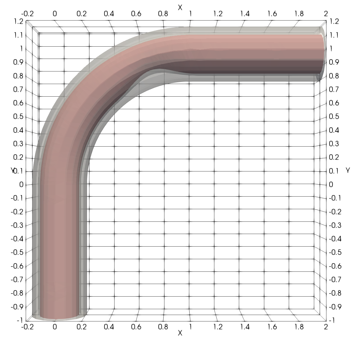
Figure 1: Computational domain showing Geometry 3 with a non-symmetric stenosis.

III.1 Geometry

The geometry of the computational domain reflects an idealized coronary artery. We show a sketch of the geometry in Figure 1. It consists of three parts, two straight and one curved tube. The straight parts are aligned with the $x-$ and $y-$ axes for inflow and outflow, respectively. The centerline of the curved section is a part of a circle with center in $(1,0,0)$ and radius $R=1$. It can be indicated as a parametrization $\psi_{C}:[0,3]\to\mathds{R}^{3}$

$$\psi_{C}(s)\coloneqq\begin{cases}(0,-1+s,0)^{T}&0\leq s\leq 1\\ (1+\cos(\pi s/2),\sin(\pi s/2),0)^{T}&1\leq s\leq 2\\ (s-1,1,0)^{T}&2\leq s\leq 3.\end{cases}$$

The fluid domain $\mathcal{F}$ is a cylinder around the centerline $\psi_{C}(s)$ with radius $r_{\mathcal{F}}=0.15\,\mathrm{cm}$. Furthermore, the solid domain (i.e. the vessel wall) is a cylindrical outer layer of width $0.06\,\mathrm{cm}$, i.e. the outer radius is given by $r_{\mathcal{S}}=0.21\,\mathrm{cm}$. These dimensions correspond the dimensions of realistic arteries.

We consider two stenotic and one non-stenotic configuration. The stenosis is modelled by a reduction of the inner radius $r_{\mathcal{F}}$ on the second part of the curved boundary. This can be described by the parametrization

$$r_{\mathcal{F}}^{sten}(s)\coloneqq\begin{cases}0.15\,\mathrm{cm}&0\leq s\leq 1.5\\ 0.15\,\mathrm{cm}-0.02\,\mathrm{cm}\big{(}\cos(4\pi s)-1\big{)}&1.5\leq s\leq 2\\ 0.15\,\mathrm{cm}&2\leq s\leq 3.\end{cases}$$

Moreover we proceed twofold. First, we consider a symmetric stenosis such that the fluid domain is a cylinder of radius $r_{\mathcal{F}}(s)$ around the centerline $\psi_{C}(s)$. Second, we modify the centerline in such a way that the stenosis is only on the inner side of the curve. This is achieved by shifting the centerline to match the radius variation, i.e.

$$\psi_{C}^{shift}(s)\coloneqq\psi_{C}(s)-r_{\mathcal{F}}^{sten}(s)\vec{\chi}(s),$$

where $\chi\omega(s)$ is the direction of the shift

$$\vec{\omega}(s)=\begin{cases}(0,-0.02\big{(}\cos(4\pi s)-1\big{)},0)&1.5\leq s\leq 2\\ (0,0,0)^{T}&\text{ elswhere }\end{cases}.$$

In both stenotic configurations, the resulting reduction of the radius equals $0.04\,\mathrm{cm}$ and the lumen area shrinks by $46\%$ from $0.15^{2}\pi\,\mathrm{cm^{2}}\approx 0.07\,\mathrm{cm^{2}}$ to $0.11^{2}\pi\,\mathrm{cm^{2}}\approx 0.038\,\mathrm{cm^{2}}$. Computational geometries are summarized in Table 1. Figure 1 shows Geometry 3.

Table 1: Summary of geometry configurations. Figure 1 shows Geometry 3.

	description	centerline	inner radius	outer radius
Geometry 1	without stenosis	$\psi_{C}(s)$	$0.15\,\mathrm{cm}$	$0.21\,\mathrm{cm}$
Geometry 2	symmetric stenosis	$\psi_{C}(s)$	$r_{\mathcal{F}}^{sten}(s)$	$0.21\,\mathrm{cm}$
Geometry 3	non-symmetric stenosis	$\psi_{C}^{shift}(s)$	$r_{\mathcal{F}}^{sten}(s)$	$0.21\,\mathrm{cm}$

III.2 Boundary conditions

The blood flow is enforced by a Dirichlet inflow condition on the inflow boundary $\Gamma_{f}^{in}$ given by

$$\Gamma_{f}^{in}=\{(x,-1,z)\in\mathds{R}^{3}\,|\,\sqrt{x^{2}+z^{2}}<0.15\,\mathrm{cm}\}.$$

We prescribe a parabolic inflow profile

$$\mathbf{v}^{in}(x,y,z,t)=v_{\text{max}}(t)\Big{(}1-\frac{x^{2}}{0.15^{2}\,\mathrm{cm^{2}}}-\frac{z^{2}}{0.15^{2}\,\mathrm{cm^{2}}}\Big{)}(0,1,0)^{T},$$

where the maximum value $v_{\text{max}}(t)$ is presented in Figure 2. The temporal inflow profile

$$v_{\text{max}}(t)=\frac{1}{28.3}\begin{cases}0.5(1.0-\cos(\pi t/0.1))3.0&0\leq t\leq 0.1\\ 3.0&0.1\leq t\leq 0.3\\ \begin{split}&5.931\\ &-1.3933\cos(2\pi 1t)+1.3532\sin(2\pi 1t)\\ &-0.9409\cos(2\pi 2t)+0.2332\sin(2\pi 2t)\\ &-0.3026\cos(2\pi 3t)-0.1190\sin(2\pi 3t)\\ &-0.2264\cos(2\pi 4t)-0.0631\sin(2\pi 4t)\\ &-0.1064\cos(2\pi 5t)-0.2137\sin(2\pi 5t)\\ &+0.0402\cos(2\pi 6t)-0.0691\sin(2\pi 6t)\\ &-0.0307\cos(2\pi 7t)-0.0451\sin(2\pi 7t)\\ &+0.0271\cos(2\pi 8t)-0.0735\sin(2\pi 8t)\end{split}&0.3\leq t\leq 3.3\end{cases}$$ (11)

is an approximation, by means of a Fourier series of order 8, of a typical coronary velocity profile provided by hemolab . The inflow profile consists of three stages:

• Ramp phase $(0\,\mathrm{s}\leq t\leq 0.1\,\mathrm{s})$ with increasing inflow rate.

• Steady phase $(0.1\,\mathrm{s}<t\leq 0.3\,\mathrm{s})$ with constant inflow rate.

• Pulsatile phase $(0.3\,\mathrm{s}<t)$ with pulsatile inflow corresponding to heartbeats.

Figure 2: Inflow profile. The exact flow rate is given in (11).

For the outflow of the fluid on $\Gamma_{f}^{out}$ in the FSI case we apply absorbing boundary conditions:

$$(\sigma_{f}^{n+1}\cdot\mathbf{n})|_{\Gamma_{out}}=\left(\left(\frac{\sqrt{\varrho_{f}}}{2\sqrt{2}}\frac{Q^{n}}{A^{n}}+\sqrt{p^{*}}\right)^{2}+p_{e}-p^{*}\right)\cdot\mathbf{n},$$ (12)

where $p*=\frac{E}{1-\nu^{2}}$. The condition is equipped with the reference pressure $p_{e}$ which is chosen such that a vascular pressure of $80\,\mathrm{mmHg}$ at $t=0.3\,\mathrm{s}$ is achieved. The absorbing condition explicitly disallows pressure waves to reenter the domain, for details see Nobile2008 .

The structure is fixed at the inflow boundary and is allowed to move in $y$-$z$ direction at the outflow boundary.

In order to compare both rigid and elastic computations, we run the FSI simulation first and then prescribe the resulting reference pressure profile $P_{ref}(t)$ at the outflow boundary in the rigid wall case such that

$$\big{\langle}\big{(}\varrho_{f}\nu_{f}\nabla\mathbf{v}_{f}-pI\big{)}\vec{n},\boldsymbol{\phi}\big{\rangle}_{\Gamma_{f}^{out}}=\big{\langle}P_{ref}(t)\vec{n},\boldsymbol{\phi}\big{\rangle}_{\Gamma_{f}^{out}}.$$

This is the usual do-nothing outflow condition including a pressure offset, see HeywoodRannacherTurek1992 .

The first two phases of (11) are designed to reach the intravascular pressure of $80\,\mathrm{mmHg}$. This procedure resembles prestressing of the vessel wall. We first start the FSI simulation on the undeformed stress free reference domain and prestress the geometry by the ramp and steady phases. The resulting geometry at $t=\mathrm{0.3}{s}$ is then extracted to compute the FSI as well as the Navier-Stokes simulation on this deformed geometry. This geometry corresponds to a reconstructed artery geometry from MRI or CT images, as during the measurements the blood flows with the pressure of at least $80\,\mathrm{mmHg}$ through the blood vessel. As the stress free reference domain is known here a priori, prestressing procedures as discussed in gee2010computational do not need to be applied.

IV Numerical approximation, solution and implementation

The realization of a numerical framework for monolithic fluid-structure interactions is very challenging and a detailed description is not possible in one manuscript. We therefore give a brief description and refer to the relevant and detailed literature. See Richter2017 for a comprehensive overview.

We employ a very strict form of the ALE formulation, where all equations are solved on the reference domain, no mesh update is used. This prevents the necessity of projections between moving meshes and also it is the only straightforward approach for obtaining higher order discretization in time RichterWick2015_time . In principle this approach allows for direct Galerkin discretizations of the monolithic variational formulation (10) and the choice of finite element spaces should be based on the following considerations

• The finite element mesh should resolve the fluid-structure interface $\mathcal{I}$ in reference framework.

• In the fluid domain, the velocity-pressure pair $V_{h}\times Q_{h}$ should fulfils the inf-sup condition to cope with the incompressibility constraint. Or, if a non-stable finite element pair is used, stabilization terms must be added. Our realization is based on equal order tri-quadratic elements for pressure and velocity, enriched with the local projection stabilization method BeckerBraack2001 .

• To reach a balanced approximation of the velocity-deformation pairing the same function space is used for the global deformation field.

To summon up, the discrete solution $U_{h}\coloneqq(\mathbf{v}_{h},\mathbf{u}_{h},p_{h})$ is found in the space $X_{h}=[V_{h}]^{3}\times[V_{h}]^{3}\times V_{h}^{f}$, where $V_{h}$ extends over the complete domain and $V_{h}^{f}$ over the fluid domain only.

In time we use a variant of the Crank-Nicolson time discretization scheme that gives better stability properties by an implicit shifting. We refer to RichterWick2015_time for details. By restricting (10) to the fully discrete setting, a system on nonlinear algebraic equations arises in each time step. As nonlinear solver we employ a Newton scheme with an analytical evaluation of the Jacobian, see Richter2012a or (Richter2017, , Section 5.2.2) for details on the derivation.

The resulting linear systems of equations are very large and extremely ill-conditioned with condition numbers that are by far larger than those of fluid and solid equation on their own, see Richter2015 ; AulisaBnaBornia2018 for numerical studies. The approximation of these systems is still a great challenge, in particular if it comes to 3d applications. Only few fast solvers for the nonlinear setting are available Richter2015 ; AulisaBnaBornia2018 ; JodlbauerLanger . Our approach is based on a multigrid solution that appears to be superior in 3d. In FailerRichter2020 we present the solution approach, which is based on a partitioning of the Jacobain based on two simple strategies:

1. Within the Navier-Stokes equations we neglect those parts of the Jacobian that come from the derivative with respect to the domain extension $\mathbf{u}_{f}$. The resulting nonlinear solver is an approximated Newton method that however still solves the original problem since the residual is exact. In (Richter2017, , Section 5.2.3) and FailerRichter2020 we have found that such an approximated Newton solver is even more efficient, despite slightly increased iteration counts. This is due to the very costly evaluation of the full Jacobian that is not required in our approach.

2. We exploit the discretization of the equation $d_{t}\mathbf{u}_{s}=\mathbf{v}_{s}$, precisely, if we consider the Crank-Nicolson scheme

   $$\mathbf{u}^{n}_{s}=\mathbf{u}^{n-1}_{s}+\frac{k}{2}\Big{(}\mathbf{v}_{s}^{n-1}+\mathbf{v}_{s}^{n}\Big{)}\eqqcolon{\cal U}(\mathbf{v}_{s}^{n};\mathbf{u}^{n-1}_{s},\mathbf{v}_{s}^{n-1}),$$

   and we replace the dependency of the solid stress tensor on the deformation by the velocity, i.e.

   $$\boldsymbol{\Sigma}_{s}(\mathbf{u}_{s})=\boldsymbol{\Sigma}_{s}\big{(}{\cal U}(\mathbf{v}_{s}^{n};\mathbf{u}^{n-1}_{s},\mathbf{v}^{n-1}_{s})\big{)}.$$

The combination of these two modifications allows for a natural splitting of the Jacobian within the multigrid smoother. Further, it allows to apply very simple iterations of Vanka-type, as smoother in the geometric multigrid preconditioner, that are easy to parallelize. In FailerRichter2020 we have demonstrated the efficiency of the approach in different 3d configurations.

The implementation is based on the finite element toolkit Gascoigne3D Gascoigne3D .

V Simulations

We finally use the presented finite element framework for a computational analysis of several hemodynamic parameters that are relevant to answer clinical questions. We focus on the dependence of these parameters on the elasticity of the vessel walls. The additional effort of fully coupled fluid-structure interactions over pure Navier-Stokes simulations is immense and should be justified by corresponding effects.

The behavior of three specific parameters is investigated. The wall shear stress (WSS) plays an eminent role in several applications. It is used as indicator to model the growth of atherosclerotic plaques YangJaegerNeussRaduRichter2015 ; RichterMizerski2020 but also when it comes to deriving measures to evaluate the risk of plaque rupture Libby2019 or the rupture of aneurysms Cebral2010 . Both the minimum wall shear stress and the distribution of the wall shear stress on the vessel walls are important measures. In Section V.1 analyze the effect of the different complexities, Navier-Stokes and fluid-structure interactions, on the WSS distribution in all three different geometries.

Furthermore we analyze the computational fractional flow reserve (cFFR). The fractional flow reserve (FFR) is a technique that measures pressure differences across a stenosis. In medical practice, the FFR is determined by inserting a catheter in the artery and measuring flow parameters at maximum blood flow. During the procedure, the tip of the catheter, where the sensor is located, is retrieved, such that measurements are available along the affected section of the vessel. Healthy vessels should give a pressure ratio close to 1. If the ratio drops below $0.8$, i.e. a $20\%$ drop in pressure, the stenosis is considered to be severe Tonino2009 . Aim of the computational fractional flow reserve is to replace the risky intervention by computer simulations based on medical imaging.

Finally, we discuss the amplitude of the pressure oscillation during one heart cycle. In clinical observation is usually observed that the amplitude significantly drops after a stenotic region in a blood vessel. By comparing Navier-Stokes simulations with coupled fluid-structure interactions, we will show that this effect can only be described by considering the fully coupled model including elastic vessel walls.

V.1 Wall shear stress (WSS)

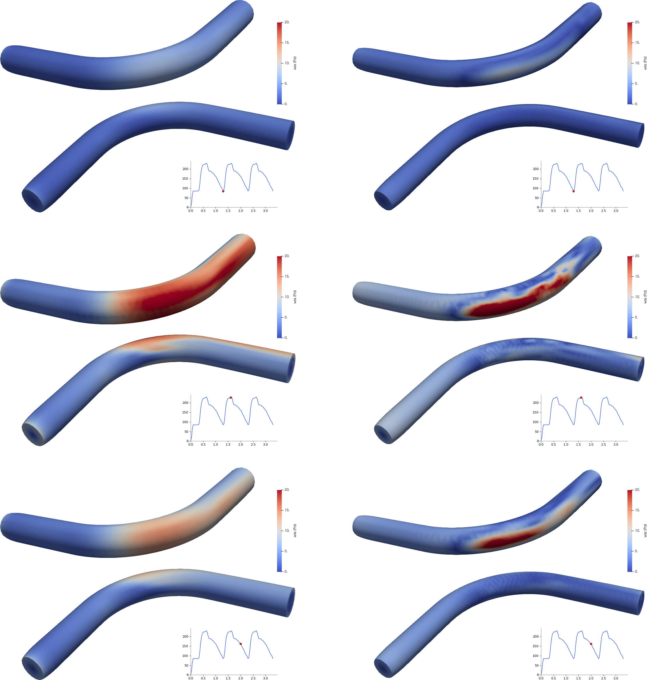
Figure 3: Wall Shear stress for Geometry 1 (without stenosis). On the left FSI right NS. We show each configuration form two different perspectives, such that inner and outer region of the curved arch are visible.

The tangential component of the surface force at the vessel wall is denoted as wall shear stress (WSS). By means of the Cauchy’s theorem we have

$$\text{WSS}=(\boldsymbol{\sigma}_{f}(\mathbf{v},p)\vec{n}\cdot\boldsymbol{\tau})\boldsymbol{\tau}=[I-\vec{n}\vec{n}^{T}]\boldsymbol{\sigma}_{f}(\mathbf{v},p)\vec{n},$$ (13)

where $\mathbf{n}$ is a unit outward normal vector to the vessel wall and $\boldsymbol{\tau}$ is corresponding tangential vector. Note that WSS is a vector and its often confused with its magnitude $|\text{WSS}|_{2}$ which is a scalar quantity denoted by $wss$.

The plots of the wall shear stress are presented on the boundary of the fluid domain, see Figure 3, Figure 5 and Figure 4. The surrounding solid is removed from these plots such that only the fluid domain is given.

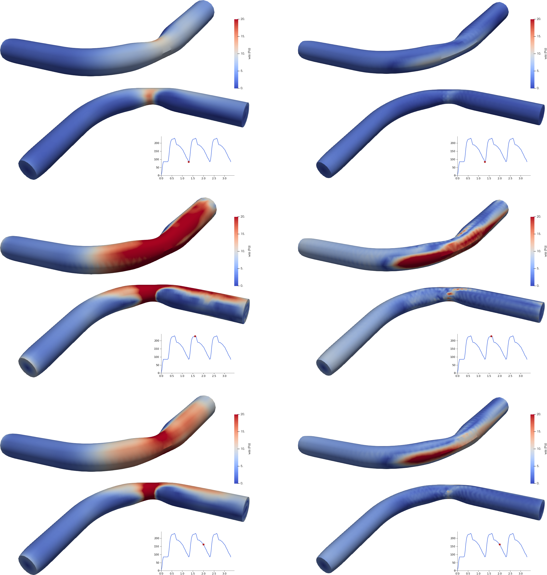
Figure 4: Wall Shear stress for Geometry 2 (non-symmetric stenosis). On the left FSI right NS. We show each configuration form two different perspectives, such that inner and outer region of the curved arch are visible.

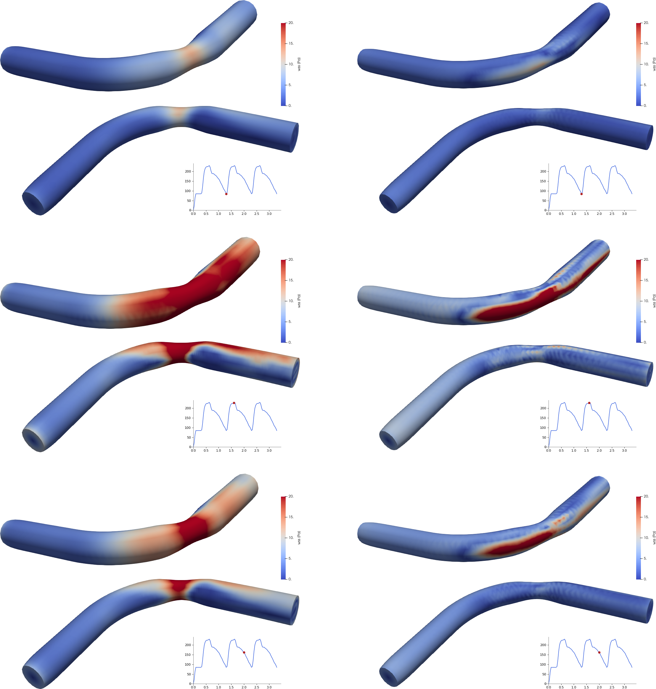
Figure 5: Wall Shear stress for Geometry 3 (symmetric stenosis). On the left FSI right NS. We show each configuration form two different perspectives, such that inner and outer region of the curved arch are visible.

We use the same scale ranging from $0\,\mathrm{Pa}$ to $20\,\mathrm{Pa}$ in all figures. The distribution of $wss$ is always presented for 3 different points in time. First, when the pulsatile flow reaches its minimum inflow pressure, then, at maximum pressure and finally for an intermediate pressure value. Each specific situation is shown from two different angles, such that the inner and outer surfaces are well visible.

Comparing the coupled fluid-structure interaction model (left) with the pure Navier-Stokes flow (right) always shows much higher wss values in the Navier-Stokes case. Regions of very high $wss$ are only found in the outer surface in the case of Navier-Stokes. In the case of the FSI model, the values are smoothly spread. In general, the vessels are widened and show a larger diameter of the lumen in the case of FSI. Prestressing of the domains for the Navier-Stokes simulations is based on the deformation resulting from the increasing inflow of the ramp phase (11) to reach pressure of $80\mathrm{mmHg}$.

Figures 5 and 4 show a shift of the wall shear stress distribution. High values are found all around the stenosed parts, on the inner and the outer surfaces of the curved areas. Again, the Navier-Stokes model is not able to yield a proper distribution of $wss$ around the cylinder surface and it only concentrates in the outer surface of the curved section.

To sum up, it appears to be important to consider elastic fluid-structure interactions, if the spatial distribution of the wall shear stress is of interest. The Navier-Stokes model is nearly unaware of the stenosis and always concentrates the WSS on the outer surface of the curved region. If rupture locations Cebral2010 or localized growth processes are of interest YangJaegerNeussRaduRichter2015 ; RichterMizerski2020 , the use of FSI is essential.

V.2 Computational fractional flow reserve (cFFR)

The computational fractional flow reserve (cFFR) is the ratio of the maximum blood pressure after the stenosis (distal) and before the stenosis (proximal). We denote by $p_{d}$ the distal pressure and by $p_{a}$ the proximal pressure such that the computational fractional flow reserve is defined by

$$\text{cFFR}=\frac{p_{d}}{p_{a}}.$$

In our configuration, compare with Figure 1, we evaluate the distal and proximal values in

$$p_{a}=p(0,0,0)\text{ and }p_{d}=p(1.7,1,0).$$ (14)

Since the cFFR varies slightly with time the maximum value over the cardiac cycle is computed. Further computational aspects of cFFR are covered by the recent benchmarking paper Carson2019 . In healthy vessels we expect $\text{cFFR}\approx 1$ and in the medical practice, a stenosis with $\text{cFFR}>0.8$ is considered to be functionally non significant Tonino2009 . No medical intervention, e.g. by placing a stent would be required.

The results of cFFR computations are presented in Table 2. The first striking observation is that the Navier-Stokes model is not able to reflect the presence of the stenosis at all. A pressure drop of about $5\%$ is observed for all configurations and is only due to the curvature of the domain. The FSI model is well able to yield $\text{cFFR}\approx 1$ in the case of the healthy configuration and shows a loss of about $5\%$ in both stenotic geometries. Based on these simulations, the stenosis would not be considered to be severe and in the need of an intervention. These results clearly show that a pure Navier-Stokes simulation is not able to serve as computational basis for replacing the medical FFR procedure by simulations.

Table 2: Results of the cFFR analysis in all three geometries, considering the fully coupled fsi model and the pure Navier-Stokes case.

	description	FSI	NS
Geometry 1	without stenosis	0.99	0.96
Geometry 2	non-symmetric stenosis	0.96	0.94
Geometry 3	symmetric stenosis	0.96	0.95

V.3 Pressure amplitude

Figure 6: Pressure waves for one cardiac cycle

The third quantity of interest is the dynamic pressure amplitude before and after the stenosis, i.e. a temporally resolved analysis of the proximal and distal pressures $p_{a}$ and $p_{d}$ evaluated in the coordinates as mentioned in (14). We study the progress of the pressure to investigate possible damping effects of a stenosis. The change of pressure profile after strongly stenotic regions, is reported as an assessment tool for cardiovascular risk Pichler2015 .

We show the evolution of the pressures $p_{a}(t)$ and $p_{d}(t)$ over the third heart beat in Figure 6. On the left, we show results for the fully coupled FSI models, on the right we give the corresponding pressure lines for the Navier-Stokes case. Comparable to the cFFR study given in the previous section, the most striking observation is the invariance of the Navier-Stokes solution to the kind of vessel geometry. For all cases, healthy vessel, centered stenosis and non symmetric stenosis, the Navier-Stokes results are nearly identical and always indicate a loss in pressure amplitude of about $7.5\%$. In contrast, the FSI solution is able to preserve the oscillation in the case of the healthy vessel and shows a drop of about $5\%$ for the two stenotic cases. A closer look reveals that the distal pressure lines are very similar in all cases. The slight oscillations in the distal pressure in case of the FSI simulation are not numerical instabilities. Instead they stem from the oscillatory behavior of the elastic vessel wall.

Finally, Table 3 collects the amplitudes before and after the stenosis. This third study also shows enormous qualitative and quantitative discrepancies between the simulation results depending on the model under consideration.

Table 3: Pressure Amplitude in $\mathrm{mmHg}$. We compare the drop of the amplitude over the stenotic region and compare the results for pure Navier-Stokes flow (left) with fully coupled fluid-structure interactions (right).

	Navier-Stokes			FSI
	proximal	distal	drop	proximal	distal	drop
Geometry 1	39.2	32.7	7.5	32.1	31.4	0.7
Geometry 2	41.0	33.4	7.6	35.8	30.5	5.3
Geometry 3	41.3	33.6	7.7	35.8	30.4	5.4

VI Conclusions

We have studied a prototypical geometry that represents a large and curved artery. Three different configurations are considered: a healthy vessel with a diameter (the lumen) of $0.15\,\mathrm{cm}$ and two cases where a stenosis is given in the curved area of the vessel. First, the stenosis is centered around the vessel centerline, finally, a shifted variant where the stenosis is concentrated on the inner surface. The blood flow is driven by a time-dependent flow rate with values that are clinically relevant. For all configurations we study the effect of the elasticity in the vessel walls, i.e. we compare a pure Navier-Stokes simulation with a fully coupled fluid-structure interaction system.

Three different indicators that are also relevant in clinical decision making are investigated: the distribution of the wall shear stress that is made responsible for stenosis growth and risk of rupture, the computational fractional flow reserve that is used to estimate the severity of a stenosis and the amplitude of the pressure oscillation that also measures the severity of a stenosis. In all cases we observe that the simple Navier-Stokes model is not able to depict the effect of the plaque. In particular the pressure lines are nearly identical for all three geometrical configurations. The FSI model is however well able to replicate clinical observations. For instance, the energy, in terms of pressure oscillations, is fully preserved throughout the curved region, if elasticity of the vessel walls is taken into account.

Although the study covers only an idealised geometry and boundary conditions, the proposed regime corresponds to physiological blood flow. Therefore, we stress that the compliance of the vessel has significant impact on clinical hemodynamical factors. In medical practise one has to be aware of the difference in the results from CFD with FSI and NS models and the limitations of the later.

Conflict of interest

The authors declare that they have no conflict of interest.

References

- (1) ADAN WEB. http://hemolab.lncc.br/adan-web/. Accessed: 2020-01-30
- (2) Aulisa, E., Bna, S., Bornia, G.: A monolithic ale newton-krylov solver with multigrid-richardson-schwarz preconditioning for incompressible fluid-structure interaction. Computers & Fluids 174, 213–228 (2018)
- (3) Balzani, D., Deparis, S., Fausten, S., Forti, D., Heinlein, A., Klawonn, A., Quarteroni, A., Rheinbach, O., Schröder, J.: Numerical modeling of fluid–structure interaction in arteries with anisotropic polyconvex hyperelastic and anisotropic viscoelastic material models at finite strains. International Journal for Numerical Methods in Biomedical Engineering 32(10), e02756 (2016). DOI 10.1002/cnm.2756. URL https://onlinelibrary.wiley.com/doi/abs/10.1002/cnm.2756. E02756 cnm.2756
- (4) Bazilevs, Y., Calo, V.M., Hughes, T.J., Zhang, Y.: Isogeometric fluid-structure interaction: theory, algorithms, and computations. Computational mechanics 43(1), 3–37 (2008)
- (5) Bazilevs, Y., Hsu, M.C., Zhang, Y., Wang, W., Kvamsdal, T., Hentschel, S., Isaksen, J.: Computational vascular fluid–structure interaction: methodology and application to cerebral aneurysms. Biomechanics and modeling in mechanobiology 9(4), 481–498 (2010)
- (6) Becker, R., Braack, M.: A finite element pressure gradient stabilization for the Stokes equations based on local projections. Calcolo 38(4), 173–199 (2001)
- (7) Becker, R., Braack, M., Meidner, D., Richter, T., Vexler, B.: The finite element toolkit Gascoigne. http://www.gascoigne.de
- (8) Blanco, P.J., Bulant, C.A., Müller, L.O., Talou, G.D.M., Bezerra, C.G., Lemos, P.A., Feijóo, R.A.: Comparison of 1d and 3d models for the estimation of fractional flow reserve. Scientific Reports 8(1) (2018). DOI 10.1038/s41598-018-35344-0. URL https://doi.org/10.1038/s41598-018-35344-0
- (9) Bluestein, D.: Utilizing computational fluid dynamics in cardiovascular engineering and medicine-what you need to know. its translation to the clinic/bedside. Artificial Organs 41(2), 117–121 (2017). DOI 10.1111/aor.12914. URL https://doi.org/10.1111/aor.12914
- (10) Carew, T.E., Vaishnav, R.N., Patel, D.J.: Compressibility of the arterial wall. Circulation research 23(1), 61–68 (1968)
- (11) Carson, J.M., Pant, S., Roobottom, C., Alcock, R., Blanco, P.J., Bulant, C.A., Vassilevski, Y., Simakov, S., Gamilov, T., Pryamonosov, R., Liang, F., Ge, X., Liu, Y., Nithiarasu, P.: Non-invasive coronary CT angiography-derived fractional flow reserve: A benchmark study comparing the diagnostic performance of four different computational methodologies. International Journal for Numerical Methods in Biomedical Engineering 35(10) (2019). DOI 10.1002/cnm.3235. URL https://doi.org/10.1002/cnm.3235
- (12) Cebral, J., Mut, F., Weir, J., Putman, C.: Quantitative characterization of the hemodynamic environment in ruptured and unruptured brain aneurysms. American Journal of Neuroradiology 32(1), 145–151 (2010). DOI 10.3174/ajnr.a2419. URL https://doi.org/10.3174/ajnr.a2419
- (13) Delfino, A., Stergiopulos, N., Moore Jr, J., Meister, J.J.: Residual strain effects on the stress field in a thick wall finite element model of the human carotid bifurcation. Journal of biomechanics 30(8), 777–786 (1997)
- (14) Donea, J.: An arbitrary lagrangian-eulerian finite element method for transient dynamic fluid-structure interactions 33, 689–723 (1982)
- (15) Failer, L., Richter, T.: A parallel newton multigrid framework for monolithic fluid-structure interactions. Journal of Scientific Computing 82(2), 28 (2020). DOI 10.1007/s10915-019-01113-y. URL https://doi.org/10.1007/s10915-019-01113-y
- (16) Fung, Y.c.: Biomechanics: mechanical properties of living tissues. Springer Science & Business Media (1993)
- (17) Gee, M.W., Förster, C., Wall, W.: A computational strategy for prestressing patient-specific biomechanical problems under finite deformation. International Journal for Numerical Methods in Biomedical Engineering 26(1), 52–72 (2010)
- (18) Gurtin, M.E., Fried, E., Anand, L.: The mechanics and thermodynamics of continua. Cambridge University Press (2010)
- (19) Heywood, J., Rannacher, R., Turek, S.: Artificial boundaries and flux and pressure conditions for the incompressible Navier-Stokes equations 22, 325–352 (1992)
- (20) Holzapfel, G.A., Gasser, T.C., Ogden, R.W.: A new constitutive framework for arterial wall mechanics and a comparative study of material models. Journal of elasticity and the physical science of solids 61(1-3), 1–48 (2000)
- (21) Jin, S., Oshinski, J., Giddens, D.P.: Effects of wall motion and compliance on flow patterns in the ascending aorta. Journal of Biomechanical Engineering 125(3), 347–354 (2003). DOI 10.1115/1.1574332. URL https://doi.org/10.1115/1.1574332
- (22) Jodlbauer, D., Langer, U., Wick, T.: Parallel block-preconditioned monolithic solvers for fluid-structure interaction problems. International Journal for Numerical Methods in Engineering 117(6), 623–643 (2019)
- (23) Liang, F., Takagi, S., Himeno, R., Liu, H.: Multi-scale modeling of the human cardiovascular system with applications to aortic valvular and arterial stenoses. Medical & Biological Engineering & Computing 47(7), 743–755 (2009). DOI 10.1007/s11517-009-0449-9. URL https://doi.org/10.1007/s11517-009-0449-9
- (24) Libby, P., Buring, J.E., Badimon, L., Hansson, G.K., Deanfield, J., Bittencourt, M.S., Tokgözoğlu, L., Lewis, E.F.: Atherosclerosis. Nature Reviews Disease Primers 5(1) (2019). DOI 10.1038/s41572-019-0106-z. URL https://doi.org/10.1038/s41572-019-0106-z
- (25) Morris, P.D., van de Vosse, F.N., Lawford, P.V., Hose, D.R., Gunn, J.P.: “virtual” (computed) fractional flow reserve. JACC: Cardiovascular Interventions 8(8), 1009–1017 (2015). DOI 10.1016/j.jcin.2015.04.006. URL https://doi.org/10.1016/j.jcin.2015.04.006
- (26) Nobile, F., Vergara, C.: An effective fluid-structure interaction formulation for vascular dynamics by generalized robin conditions. SIAM Journal on Scientific Computing 30(2), 731–763 (2008). DOI 10.1137/060678439. URL https://doi.org/10.1137/060678439
- (27) Perktold, K., Rappitsch, G.: Computer simulation of local blood flow and vessel mechanics in a compliant carotid artery bifurcation model. Journal of Biomechanics 28(7), 845 – 856 (1995). DOI https://doi.org/10.1016/0021-9290(95)95273-8. URL http://www.sciencedirect.com/science/article/pii/0021929095952738
- (28) Pichler, G., Martinez, F., Vicente, A., Solaz, E., Calaforra, O., Redon, J.: Pulse pressure amplification and its determinants. Blood Pressure 25(1), 21–27 (2015). DOI 10.3109/08037051.2015.1090713. URL https://doi.org/10.3109/08037051.2015.1090713
- (29) Quarteroni, A., Tuveri, M., Veneziani, A.: Computational vascular fluid dynamics: problems, models and methods. Computing and Visualization in Science 2(4), 163–197 (2000). DOI 10.1007/s007910050039. URL https://doi.org/10.1007/s007910050039
- (30) Richter, T.: Goal-oriented error estimation for fluid–structure interaction problems. Computer Methods in Applied Mechanics and Engineering 223-224, 28–42 (2012). DOI 10.1016/j.cma.2012.02.014. URL https://doi.org/10.1016/j.cma.2012.02.014
- (31) Richter, T.: A monolithic geometric multigrid solver for fluid-structure interactions in ALE formulation. International Journal for Numerical Methods in Engineering 104(5), 372–390 (2015). DOI 10.1002/nme.4943. URL https://doi.org/10.1002/nme.4943
- (32) Richter, T.: Fluid-structure Interactions. Models, Analysis and Finite Elements, Lecture notes in computational science and engineering, vol. 118. Springer (2017)
- (33) Richter, T., Mizerski, J.: The candy wrapper problem - a temporal multiscale approach for pde/pde systems. In: ENUMATH 2019. Springer (2020)
- (34) Richter, T., Wick, T.: On time discretizations of fluid-structure interactions. In: T. Carraro, M. Geiger, S. Körkel, R. Rannacher (eds.) Multiple Shooting and Time Domain Decomposition Methods, Contributions in Mathematical and Computational Science, vol. 9, pp. 377–400. Springer (2015)
- (35) Steinman, D.A.: Assumptions in modelling of large artery hemodynamics, pp. 1–18. Springer Milan, Milano (2012)
- (36) Taylor, C.A., Draney, M.T., Ku, J.P., Parker, D., Steele, B.N., Wang, K., Zarins, C.K.: Predictive medicine: Computational techniques in therapeutic decision-making. Computer Aided Surgery 4(5), 231–247 (1999). DOI 10.3109/10929089909148176. URL https://doi.org/10.3109/10929089909148176. PMID: 10581521
- (37) Tonino, P.A., Bruyne, B.D., Pijls, N.H., Siebert, U., Ikeno, F., van ’t Veer, M., Klauss, V., Manoharan, G., Engstrom, T., Oldroyd, K.G., Lee, P.N.V., MacCarthy, P.A., Fearon, W.F.: Fractional flow reserve versus angiography for guiding percutaneous coronary intervention. New England Journal of Medicine 360(3), 213–224 (2009). DOI 10.1056/nejmoa0807611. URL https://doi.org/10.1056/nejmoa0807611
- (38) Torii, R., Keegan, J., Wood, N.B., Dowsey, A.W., Hughes, A.D., Yang, G.Z., Firmin, D.N., Thom, S.A.M., Xu, X.Y.: Mr image-based geometric and hemodynamic investigation of the right coronary artery with dynamic vessel motion. Annals of Biomedical Engineering 38(8), 2606–2620 (2010). DOI 10.1007/s10439-010-0008-4. URL https://doi.org/10.1007/s10439-010-0008-4
- (39) Yang, Y., Jäger, W., Neuss-Radu, M., Richter, T.: Mathematical modeling and simulation of the evolution of plaques in blood vessels. J. of Math. Biology 72(4), 973–996 (2016)