Relating the structure of dark matter halos to their assembly and environment

Abstract

We use a large $N$-body simulation to study the relation of the structural properties of dark matter halos to their assembly history and environment. The complexity of individual halo assembly histories can be well described by a small number of principal components (PCs), which, compared to formation times, provide a more complete description of halo assembly histories and have a stronger correlation with halo structural properties. Using decision trees built with the random ensemble method, we find that about $60\%$, $10\%$, and $20\%$ of the variances in halo concentration, axis ratio, and spin, respectively, can be explained by combining four dominating predictors: the first PC of the assembly history, halo mass, and two environment parameters. Halo concentration is dominated by halo assembly. The local environment is found to be important for the axis ratio and spin but is degenerate with halo assembly. The small percentages of the variance in the axis ratio and spin that are explained by known assembly and environmental factors suggest that the variance is produced by many nuanced factors and should be modeled as such. The relations between halo intrinsic properties and environment are weak compared to their variances, with the anisotropy of the local tidal field having the strongest correlation with halo properties. Our method of dimension reduction and regression can help simplify the characterization of the halo population and clarify the degeneracy among halo properties.

1 Introduction

In the concordant $\rm\Lambda$ cold dark matter ($\rm\Lambda$CDM) cosmology, dark matter halos, the dense clumps formed through gravitational collapse of the initial density perturbations, are the basic building blocks of the cosmic web. The formation history of a halo not only depends on the properties of the local density field, but may also be affected by the environment within which it forms. Since galaxies are believed to form in the gravitational potential wells of dark matter halos, the halo population provides a link between the dark and luminous sectors of the universe. Consequently, the understanding of the formation, structure, and environment of dark matter halos and their relations to each other has long been considered one of the most important parts of galaxy formation (e.g. Mo et al., 2010).

Dark matter halos are diverse in their structure, mass assembly history (MAH), and interaction with the large-scale environment. Among the structural properties of dark matter halos, the most important ones are the concentration parameter (Navarro et al., 1997), the spin parameter (Bett et al., 2007; Gao & White, 2007; MacCiò et al., 2007), and the shape parameter (Jing & Suto, 2002; Bett et al., 2007; Hahn et al., 2007; MacCiò et al., 2007). In $N$-body simulations, halo concentration is found to be correlated with halo mass and MAH (Navarro et al., 1997; Jing, 2000; Wechsler et al., 2002; Zhao et al., 2003a, b; MacCiò et al., 2007, 2008; Zhao et al., 2009; Ludlow et al., 2014, 2016). The spin and shape parameters are also found to be related to other properties, such as halo mass and large-scale environment (MacCiò et al., 2007, 2008; Wang et al., 2011). However, these relations have large variance and remain poorly quantified.

The mass assembly histories of halos in general are complex. In the literature, a common practice is to focus on the main-branch assembly histories, ignoring other branches (e.g., van den Bosch, 2002; Wechsler et al., 2002; Zhao et al., 2003a, b; Ludlow et al., 2013, 2014, 2016). Attempts have been made to describe the histories of individual halos with simple parametric forms (van den Bosch, 2002; Wechsler et al., 2002; Zhao et al., 2003a, b; Tasitsiomi et al., 2004; McBride et al., 2009; Correa et al., 2015; Zhao et al., 2009). These simple models are useful in providing some crude description of halo assembly histories, but are not meant to give a complete characterization. Because of this, a variety of formation times have also been defined to characterize different aspects of the assembly histories of dark matter halos (see, e.g., Li et al., 2008, for a review). These formation times, usually degenerate among themselves, again only provide an incomplete set of information about the full assembly history.

The environment of a halo is also complex. To the lowest order, the average mass density around individual halos in a population can be used to characterize the distribution of the population relative to the underlying mass density field. In general, the spatial distribution of halos (halo environment) can depend on the intrinsic properties of the halos. The mass dependence, often called the halo bias (Mo & White, 1996), is a natural outcome of the formation of halos in a Gaussian density field (Sheth et al., 2001; Zentner, 2007). Furthermore, correlations have also been found between halo bias and halo assembly history. Halos, particularly low-mass ones, that formed earlier tend to be more strongly clustered (Gao et al., 2005; Gao & White, 2007; Li et al., 2008). This phenomenon is now referred to as the halo assembly bias, and various studies have been carried out to understand its origin (Sandvik et al., 2007; Wang et al., 2007, 2009; Zentner, 2007; Dalal et al., 2008; Desjacques, 2008; Lazeyras et al., 2017). In addition to assembly history, halo bias has also been analyzed in its dependencies on other halo properties, such as halo concentration (Wechsler et al., 2006; Jing et al., 2007), substructure occupation (Wechsler et al., 2006; Gao & White, 2007), halo spin (Bett et al., 2007; Gao & White, 2007; Hahn et al., 2007; Wang et al., 2011), and halo shape (Hahn et al., 2007; Faltenbacher & White, 2010; Wang et al., 2011). These dependencies are collectively referred to as the “secondary bias”, and sometimes also as the “assembly bias”, presumably because these intrinsic properties may be related to halo formation.

Since halo properties are intrinsically correlated, it is necessary to investigate the joint distribution of different properties. Along this line, Jeeson-Daniel et al. (2011) used rank-based correlation coefficients to quantify the correlation between pairs of halo properties. Lazeyras et al. (2017) investigated halo bias as a function of two halo properties. They found that in all combinations of halo properties considered, halo bias can change with the second parameter when the first is fixed, and that the maximum of the halo bias occurs for halos with special combinations of the halo properties. For the environment, new parameters have also been introduced in addition to the local mass density. For example, Wang et al. (2011) used local tidal fields to represent the halo environment, and Salcedo et al. (2018) used the closest distance to a neighbor halo more massive than the halo in question. However, it is still unclear which quantity is the driving force of halo bias and which combination of bias sources can provide a more complete representation. Answering these questions requires more advanced statistical tools to measure the capability of models to fit the data and to identify hidden degeneracy between model parameters.

Some statistical tools are available for such investigations. For unsupervised learning tasks, the Principal Component Analysis (PCA) is a powerful tool to determine the main sources that contribute to the sample scatter and decompose the sample scatter along principal axes. For example, Wong & Taylor (2012) used this technique to reduce the dimension of halo MAH, while Cohn & van de Voort (2015) and Cohn (2018) applied the PCA to model the star formation history of galaxies. Jeeson-Daniel et al. (2011) used PCA to study the correlation of dark matter halo properties. For supervised learning tasks, the Ensemble of Decision Trees (EDT) or Random Forest (RF) is capable of both classification and regression. This method can also capture the nonlinear patterns, effectively reducing model complexity and discovering the dominant factors in target variables. RF has been widely used recently, for example, in identifying galaxy merger systems (de los Rios et al., 2016), in galaxy morphology classification (Dobrycheva et al., 2017; Sreejith et al., 2018), in predicting neutral hydrogen contents of galaxies (Rafieferantsoa et al., 2018), in determining structure formation in $N$-body simulations (Lucie-Smith et al., 2018, see also Lucie-Smith et al. (2019) for boosted trees), in measuring galaxy redshifts (Stivaktakis et al., 2018), in classifying star-forming versus quenched populations (Bluck et al., 2019), in identifying the best halo mass proxy in observation (Man et al., 2019), and in estimating the star formation rate and stellar mass of galaxies (Bonjean et al., 2019).

In this paper, we use both the PCA and the RF regressor to investigate the dependence of halo structural properties on halo assembly history and environment. The paper is organized as follows. In §2 we describe the simulation and the halo quantities to be analyzed. In §3 we demonstrate how to use PCA to extract information about halo assembly history. In §4 we relate halo structure properties to assembly history and environment, identifying the dominating factors that determine halo properties. We also investigate the dependence of halo structure and assembly history on halo environment and halo mass. We summarize our main results in §5.

2 Simulation and Halo Quantities

2.1 The Simulation

Table 1: Samples Used in Our Analysis. The four columns are sample identifier, number of halos, halo mass range, and usage, respectively. The exact sample definitions can be found in §2.1.

Sample	${\rm N_{halo}}$	$M_{\rm halo}/[\,h^{-1}{\rm M_{\odot}}]$	Usage
$\rm S_{1}$	2000	$10^{[11,11.2]}$	Samples with constrained halo masses. Used in §3.1.
$\rm S_{2}$	1000	$10^{[12,12.2]}$
$\rm S_{3}$	500	$10^{[13,13.2]}$
$\rm S_{4}$	500	$10^{[14,14.5]}$
$\rm S_{c}$	10000	$\geq 10^{11}$	Mass-limited sample. Used in §3.1.
$\rm S_{c}^{\prime}$	2335	$\geq 5\times 10^{11}$	Subsample of $\rm S_{c}$, with all halo properties well-defined. Used in §3.2, §4.1, §4.2.
$\rm S_{L}$	94524	$10^{[11,14.6]}$	The ’larger’ sample for binning statistics. Used in §4.3, §4.4.

The $N$-body simulation used here is the ELUCID simulation carried out by Wang et al. (2016) using L-GADGET code, a memory-optimized version of GADGET-2 (Springel, 2005). The simulation uses $3072^{3}$ dark matter particles, each with a mass $3.08\times 10^{8}\,h^{-1}{\rm M_{\odot}}$, in a periodic cubic box of $500$ comoving $\,h^{-1}{\rm{Mpc}}$ on a side. The cosmology parameters used are those based on WMAP5 (Dunkley et al., 2009): a $\Lambda$CDM universe with density parameters $\Omega_{\rm K,0}=0$, $\Omega_{\rm M,0}=0.258$, $\Omega_{\rm B,0}=0.044$ and $\Omega_{\rm\Lambda,0}=0.742$, a Hubble constant $H_{0}=100\ h\,{\rm km\,s^{-1}\,Mpc^{-1}}$ with $h=0.72$, and a Gaussian initial density field with power spectrum $P(k)\propto k^{n}$ with $n=0.96$ and an amplitude specified by $\sigma_{8}=0.80$. A total of 100 snapshots, uniformly spaced in $\log(1+z)$ between $z=18.4$ and $z=0$, are taken and stored.

Halos and subhalos with more than 20 particles are identified by the friends-of-friends (FoF; see, e.g., Davis et al., 1985) and SUBFIND (Springel, 2005) algorithms. Halos and subhalos among different snapshots are linked to build halo merger trees. Halo virial radius $R_{\rm vir}$ is related to halo mass, $M_{\rm halo}$, through

$$M_{\rm halo}={4\pi R_{\rm vir}^{3}\over 3}\Delta_{\rm vir}{\overline{\rho}}\,,$$ (1)

where ${\overline{\rho}}$ is the mean density of the universe, and $\Delta_{\rm vir}$ is an overdensity obtained from the spherical collapse model (Bryan & Norman, 1998). The center of a halo is assumed to be the position of the most bound particle of the main subhalo. Halo mass $M_{\rm halo}$ is computed by summing over all the particles enclosed within $R_{\rm vir}$. The virial velocity, $V_{\rm vir}$, is defined as $V_{\rm vir}=\sqrt{GM_{\rm halo}/R_{\rm vir}}$, where $G$ is the gravitational constant. We use halos with masses $\geq 10^{10}\,h^{-1}{\rm M_{\odot}}$ directly from the simulation, and we use Monte-Carlo-based merger trees to extend the mass resolution of trees down to $10^{9}\,h^{-1}{\rm M_{\odot}}$ (see Chen et al., 2019).

From the halo merger tree catalog constructed above, we form four samples according to halo mass: ${\rm S_{1}}$ contains 2000 halos with $10^{11}\leq M_{\rm halo}/\,h^{-1}{\rm M_{\odot}}\leq 10^{11.2}$; ${\rm S_{2}}$ contains 1000 halos with $10^{12}\leq M_{\rm halo}/\,h^{-1}{\rm M_{\odot}}\leq 10^{12.2}$; ${\rm S_{3}}$ contains 500 halos with $10^{13}\leq M_{\rm halo}/\,h^{-1}{\rm M_{\odot}}\leq 10^{13.2}$; and ${\rm S_{4}}$ contains 500 halos with $10^{14}\leq M_{\rm halo}/\,h^{-1}{\rm M_{\odot}}\leq 10^{14.5}$. We also construct a complete sample, ${\rm S_{c}}$, which contains 10,000 halos with $M_{\rm halo}/\,h^{-1}{\rm M_{\odot}}\geq 10^{11}$ to represent the total halo population. All halos in samples $\rm S_{1}$, $\rm S_{2}$, $\rm S_{3}$, $\rm S_{4}$ and $\rm S_{c}$ are randomly selected from simulated halos at $z=0$. When halos need to be divided into subsamples according to some properties, the sample size of $\rm S_{c}$ may be insufficient. In this case, we construct a larger sample by the following steps. Starting from all simulated halos at $z=0$ with $M_{\rm halo}/\,h^{-1}{\rm M_{\odot}}=10^{11}$ - $10^{14.6}$, we divide them into mass bins of width of $0.3\,{\rm dex}$. If the number of halos in a bin exceeds 10,000, we randomly choose 10,000 from them; otherwise all halos in this mass bin are kept. This gives a sample of 94,524 halos, which is referred to as sample $\rm S_{L}$. Due to the mass resolution of the ELUCID simulation, some properties of small halos cannot be derived reliably. Whenever these properties are needed, we use another halo sample, ${\rm S_{c}^{\prime}}$, which contains all halos with $M_{\rm halo}\geq 5\times 10^{11}\,h^{-1}{\rm M_{\odot}}$ in sample $\rm S_{c}$.

Note that halos with recent major mergers may have structural properties that are very different from virialized halos, and including them in our sample will significantly increase the variance of halo properties, thereby affecting the statistics derived from the sample. We use the criteria described in Appendix C to exclude those ’unrelaxed’ halos.

All of the samples used in this paper are summarized in the Table 1. Note that we use only a fraction of all halos in a given mass range available in the simulation to save computational time. We have made tests using larger samples to confirm that the samples we use are sufficiently large to obtain robust results.

2.2 Halo assembly history

Following the literature (e.g., van den Bosch, 2002; Wechsler et al., 2002; Zhao et al., 2003a, b), we define the halo MAH of a halo as the main-branch mass $M_{z}$ as a function of redshift $z$ in the halo merger tree rooted in that halo. Based on a theoretical consideration of halo formation (e.g. Zhao et al., 2009), we use the following quantity as the mass variable:

$$s(z)=\sigma(M_{\rm 0})/\sigma(M_{z}),$$ (2)

where $\sigma(M)$ is the rms of the $z=0$ linear density field at the mass scale $M$. Similarly, we use

$$\delta_{\rm c}(z)=\delta_{\rm c,0}/D(z),$$ (3)

as the time variable, where $\delta_{\rm c,0}=1.686$ is the critical overdensity for spherical collapse, and $D(z)$ is the linear growth factor at $z$. We use the transfer function given by Eisenstein & Hu (1998) and the linear growth factor $D(z)$ from Carroll et al. (1992). These definitions for the mass and time variables are well motivated by the self-similar behavior of halo formation expected in the Press-Schechter formalism (e.g. Press & Schechter, 1974; Mo et al., 2010).

Thus, in our definition, the MAH of a halo is a vector $\mathrm{\bf s}=(s(z_{1}),\ s(z_{2}),\ ...,\ s(z_{\rm M}))^{\rm T}$, with each of its elements being the main-branch mass at a snapshot in the merger tree . Such a high-dimensional vector is obviously too complex to be useful in characterizing the formation of a halo. To overcome this problem, a common practice is to characterize the full MAH by a set of formation times (e.g., Li et al., 2008). In our analysis, we will use both the formation times and the principal components (PCs; see §3) to reduce the dimension of the MAH.

The MAH introduced above only uses the main branch of a halo merger tree, and thus it may potentially lose important information about the formation of a halo. However, our tests including the side branches (e.g., by modeling the assembly history with the progenitor mass distribution, as used in Parkinson et al. (2008)) showed that it does not provide important information about halo structural properties. We therefore only use the main-branch assembly history for our analysis.

2.3 Halo concentration

Dark matter halo profiles are usually modeled by a universal two-parameter form - the Navarro-Frenk-White (NFW) profile (Navarro et al., 1997),

$$\rho_{\rm NFW}(r)={{\delta\rho_{\rm crit}}\over{(r/r_{\rm s})(1+r/r_{\rm s})^{2}}},$$ (4)

where $\rho_{\rm crit}=3H^{2}/(8\pi G)$ is the critical density of the universe. This profile is specified by a dimensionless amplitude, $\delta$, and a scale radius, $r_{\rm s}$. The scale radius is usually expressed in terms of the virial radius, $R_{\rm vir}$, through a concentration parameter, $c\equiv R_{\rm vir}/r_{\rm s}$. Since both $\overline{\rho}$ and $\Delta_{\rm vir}$ in equation (1) are known for a given cosmology, the profile of a halo can be specified by the parameter pair $(M_{\rm halo},\,c)$, where the halo mass $M_{\rm halo}$ is defined in 2.1.

We obtain the concentration parameter of a halo through the following steps (see Bhattacharya et al., 2013):

• We divide the volume centered on a halo into $N_{\rm r}=20$ radial bins equally spaced between 0 and $R_{\rm vir}$ (see 2.1 for definitions of halo center and radius), and calculate the mass within each bin $i$, $M_{i}$, using the number of particles in the bin.

• We compute the mass expected from the NFW profile in this bin, $M_{i,{\rm NFW}}(c)$, assuming a concentration parameter $c$.

• We define an objective function, $\chi^{2}(c)$, to be minimized as

  $$\chi^{2}(c)=\sum_{i=1}^{N_{\rm r}}\frac{[M_{i}-M_{i,{\rm NFW}}(c)]^{2}}{M_{i}^{2}/n_{i}}.$$ (5)

• We minimize the objective function to find the best-fit concentration parameter $c_{\rm fit}={\rm argmin}_{c}\chi^{2}(c)$.

In what follows, we will drop the subscript ’fit’ and use $c$ to denote the concentration parameter obtained this way. As tested by Bhattacharya et al. (2013), changing the radius range and binning scheme in the fitting only introduces a negligible difference in $c$. According to our tests, our results presented in the following sections are also insensitive to such changes.

2.4 Halo axis ratio

We model the mass distribution in a dark matter halo with an ellipsoid and use its axis ratio to characterize its shape. Our modeling consists of the following steps (see MacCiò et al., 2007):

• We start from a FOF halo and calculate the spatial position ${\rm d}\mathrm{{\bf r}}_{i}$ relative to the center of mass for each particle linked to the halo. The inertia tensor $\mathcal{M}$ of the halo is given by the dyadic of ${\rm d}\mathrm{{\bf r}}_{i}$ summing over all of the ${\rm N_{p}}$ particles in that halo:

  $$\mathcal{M}=\sum_{i=1}^{\rm N_{p}}m_{i}{\rm d}\mathrm{{\bf r}}_{i}{\rm d}\mathrm{{\bf r}}_{i}^{\rm T},$$ (6)

  where $m_{i}$ is the particle mass.

• We calculate the eigenvalues $\lambda_{\mathcal{M},i}$ and eigenvectors $v_{\mathcal{M},i}\,(i=1,2,3)$ of $\mathcal{M}$, and rank the eigenvalues in descending order: $\lambda_{\mathcal{M},1}\geq\lambda_{\mathcal{M},2}\geq\lambda_{\mathcal{M},3}$. So defined, $v_{\mathcal{M},i}$ gives the axis direction of the inertia ellipsoid, and $a_{\mathcal{M},i}$ = $\sqrt{\lambda_{\mathcal{M},i}}$ gives the length of the corresponding axis.

• We define the axis ratio $q_{\rm axis}$ of the halo as

  $$q_{\rm axis}=\frac{a_{\mathcal{M},2}+a_{\mathcal{M},3}}{2a_{\mathcal{M},1}}.$$ (7)

  So defined, $q_{\rm axis}=1$ for a spherical halo, and close to zero if the halo is very elongated along the major axis.

2.5 Halo spin

Following Bullock et al. (2001), we define the spin parameter of a halo as

$$\lambda_{\rm s}\equiv\frac{\left\lVert\mathrm{{\bf j}}\right\rVert}{\sqrt{2}M_{\rm halo}R_{\rm vir}V_{\rm vir}},$$ (8)

where $M_{\rm halo}$, $R_{\rm vir}$ and $V_{\rm vir}$ are, respectively, the halo mass, virial radius, and virial velocity defined in §2.1. The total angular momentum $\mathrm{{\bf j}}$ is defined as

$$\mathrm{{\bf j}}=\sum_{i=1}^{\rm N_{p}}m_{i}{\rm d}\mathrm{{\bf r}}_{i}\times{\rm d}\mathrm{{\bf v}}_{i},$$ (9)

where $m_{i}$ is the particle mass, and ${\rm d}\mathrm{{\bf r}}_{i}$ and ${\rm d}\mathrm{{\bf v}}_{i}$ are particle position and velocity vectors relative to the center of mass, respectively. The summation is over all of the $\rm N_{p}$ particles linked in the FOF halo.

2.6 Environmental quantities

Many definitions can be found in the literature to characterize the environment of a halo at different scales, traced by different objects, and including or excluding the halo itself (see Haas et al. (2012) for a review). Here we define two quantities to describe the environment in which a halo resides: the density contrast as specified by the bias factor, and the tidal tensor. These quantities are computed directly from the N-body simulation.

Firstly we follow Mo & White (1996) to define halo bias $b$ as the ratio between the halo-matter cross-correlation function and the matter-matter autocorrelation function. For each simulated halo $i$, we calculate its bias $b_{i}$ by

$$b_{i}=\frac{\xi_{{\rm hm},i}(R)}{\xi_{\rm mm}(R)},$$ (10)

where $\xi_{{\rm hm},i}(R)$ is the overdensity centered at halo $i$ at a radius $R$, and $\xi_{{\rm mm}}(R)$ is the matter-matter auto-correlation function at the same radius in the simulation at the redshift in question. On linear scales, the bias factor is expected to depend only on halo mass, independent of $R$. We have checked the values of $b$ on different scales and found that the bias factor is almost constant at $R>5\,h^{-1}{\rm{Mpc}}$. In the following, we compute both $\xi_{{\rm hm},i}$ and $\xi_{\rm mm}$ for $R$ between $5$ and $15\,h^{-1}{\rm{Mpc}}$ at $z=0$, and we obtain the corresponding local linear bias $b_{i}$ for each halo using the above equation.

For the tidal field, we follow Ramakrishnan et al. (2019) and define the halo environment in the following steps: we first divide the simulation box into a sufficiently fine grid (of $\rm N_{cell}^{3}$ grid points), and compute the density field $\rho(\mathrm{{\bf x}})$ on each grid point using the clouds-in-cell method (Hockney & Eastwood, 1988). To describe the environment of a given halo, the density field is smoothed on some scale $R_{\rm sm}$ with a Gaussian kernel. We then compute the potential field $\Phi(\mathrm{{\bf x}})$ by solving the Poisson equation

$$\nabla^{2}\Phi(\mathrm{{\bf x}})=4\pi G{\overline{\rho}}\delta(\mathrm{{\bf x}}),$$ (11)

where $\delta(\mathrm{{\bf x}})=\rho(\mathrm{{\bf x}})/\overline{\rho}-1$ is the overdensity and $\overline{\rho}$ the mean density of the universe. Next we obtain the tidal field $\mathcal{T}(\mathrm{{\bf x}})$ through

$$\mathcal{T}(\mathrm{{\bf x}})=\nabla\nabla\Phi(\mathrm{{\bf x}}).$$ (12)

Finally, we solve the eigenvalue problem of the tidal tensor at each grid point to find the eigenvalues $\lambda_{1}(\mathrm{{\bf x}})$, $\lambda_{2}(\mathrm{{\bf x}})$, $\lambda_{3}(\mathrm{{\bf x}})$ (ranked in a descending order).

With all these, we obtain four environmental quantities for each halo: the local bias factor and the three eigenvalues of the tidal tensor: $\lambda_{i}$ ($i=1,2,3$). We follow the definition in Ramakrishnan et al. (2019) to define the local tidal anisotropy at each halo’s position as

$$\alpha_{\mathcal{T}}=\sqrt{q^{2}}/(1+\delta),$$ (13)

where $q^{2}=\frac{1}{2}[(\lambda_{1}-\lambda_{2})^{2}+(\lambda_{2}-\lambda_{3})^{2}+(\lambda_{1}-\lambda_{3})^{2}]$ is the halocentric tidal shear, and $\delta=\lambda_{1}+\lambda_{2}+\lambda_{3}$ is the local overdensity. For our applications, we choose $R_{\rm sm}=4R_{\rm vir}$, although we have checked that our conclusion does not change significantly by using other values of $R_{\rm sm}$. We use $\rm N_{cell}=2560$, which is sufficiently fine for computing $\alpha_{\mathcal{T}}$ for the smallest halo in our sample.

In Table 2, we summarize the halo assembly, structure, and environmental properties used in our analysis.

Table 2: Summary of Halo Properties Studied in This paper. Detail descriptions of halo MAH PCs and structural and environmental quantities can be found in §2 and §3.1.

Property Type	Notation	Meaning
Assembly History	${\rm PC}_{{\rm MAH},i}$	$i$th principal component of MAH
Structure	$c$	concentration parameter of the NFW profile
	$\lambda_{\rm s}$	dimensionless spin parameter
	$q_{\rm axis}$	axes ratio of inertia momentum
Environment	$b$	halo bias factor
	$\alpha_{\mathcal{T}}$	tidal anisotropy

3 Characterizing Halo Assembly History with PCs

Because many parameters can be defined to characterize various aspects of the halo assembly history (e.g., different formation times), it is not feasible to use all of them directly to study the relationship between halo assembly and other halo properties. In this section, we describe a method that can be used to effectively reduce the dimension of the halo assembly history, which has some advantages over using formation times.

We use the PCA described in Appendix A.1 to reduce the dimension of the MAH. In this section we will show the advantages of using such a method in the following two aspects. (1) The PCs capture the most variance among all linear, low-dimension representations and are the best in reducing the reconstruction error. We will demonstrate their power in representing the halo MAH. (2) The PCs are tightly correlated with some formation times widely used in the literature, which helps clarify the types of information PCs contain. In the next section (§4), we will show that PCs are strongly correlated with halo structural properties, which helps us understand the origin of such properties. All these indicate that PCs are not only mathematically optimized approximations to the MAH but also have clear physical meanings.

3.1 PCs of Halo Assembly Histories

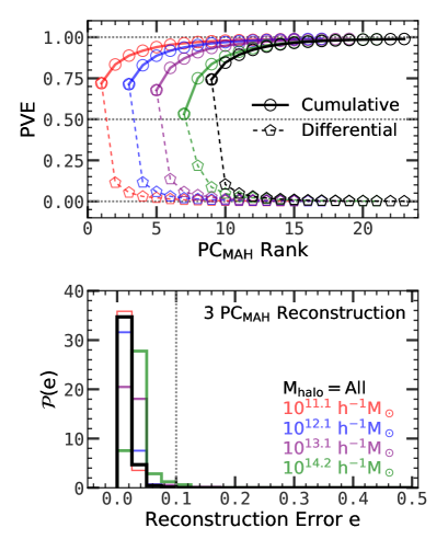
Figure 1: The performance of PCA on a halo MAH. Top: PVEs and their cumulative version (see Appendix A.1 for definitions). Each curve is horizontally offset increasingly by 2 for clarity. Bottom: distribution of reconstruction error $e$ using the first three MAH PCs. In both panels, five samples, $\rm S_{1}$, $\rm S_{2}$, $\rm S_{3}$, $\rm S_{4}$, $\rm S_{c}$, with different halo mass selections (see §2.1 and Table 1) indicated in the lower panel, are presented.

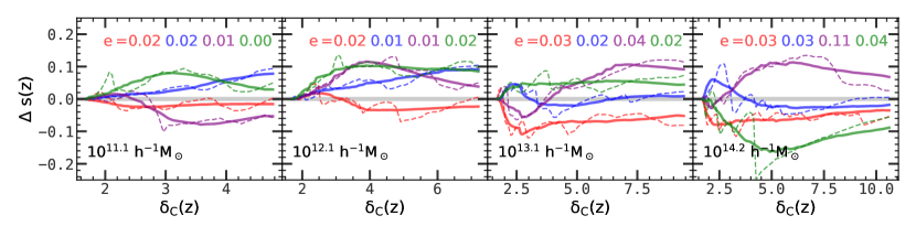
Figure 2: Reconstructed MAHs of example halos (solid) compared with the real ones (dashed). Four panels present halos with different masses indicated in each panel. In each case, the MAHs are reconstructed from the first three PCs. The reconstruction error $e$ for each halo is also presented.

For a given sample of $N$ halos, the MAHs are represented by $\mathrm{\bf S}=(\mathrm{\bf s}_{1},\ \mathrm{\bf s}_{2},\ ...,\ \mathrm{\bf s}_{\rm N})^{\rm T}$, where $\mathrm{\bf s}_{i}$ is the MAH of the $i$th halo, as defined in §2.2. In simulation, the MAH of a halo is not traced below the mass resolution of the simulation. Halos of different mass therefore may be traced down to different snapshots, resulting in different lengths of the vector $\mathrm{\bf s}_{i}$. For a given sample, we choose a snapshot where $90\%$ of the MAHs can be traced back to this time. MAHs extending beyond this snapshot are truncated, and MAHs that are terminated before this snapshot are padded with $0$. In this way, all of the $\mathrm{\bf s}_{i}$ will have the same length, $M$, suitable for PCA. After applying the PCA to $\mathrm{\bf S}$, the $\mathrm{\bf s}$ for each halo is transformed into a new coordinate system, producing a new vector that consists of a series of PCs, $\mathrm{\bf pc}_{\rm MAH}=({\rm PC}_{\rm MAH,1},\,{\rm PC}_{\rm MAH,2},\,...,\,{\rm PC}_{\rm MAH,M})$. In terms of the capability of capturing sample variance and reducing reconstruction errors, PCA is theoretically the optimal linear method. Thus, if the assembly histories of halos have some dominating modes, they are expected to be captured by the PCA.

The upper panel of Figure 1 shows the PVE and CPVE curves (see Appendix A.1 for definitions) for the PCs of the five samples, ${\rm S_{1}}$, ${\rm S_{2}}$, ${\rm S_{3}}$, ${\rm S_{4}}$ and ${\rm S_{c}}$, defined in §2.1 (see also Table 1). Since the proportional explained variance (PVE) measures the fraction of sample variance explained by a PC, it is clear that the first several PCs, among all cases, can capture most of the variance in the halo MAH ($>80\%$ by using the first three PCs). This demonstrates that strong degeneracy exists in the MAH of individual halos, suggesting that the assembly history can be described by using only a few eigen-modes. As shown by the CPVE curve, using a single parameter is insufficient to describe the MAH. It can at most explain as much variance as ${\rm PC}_{1}$, which is $55\%$ for the most massive halos ($\approx 10^{14}\,h^{-1}{\rm M_{\odot}}$), and $70\%$ for the smallest halos ($\approx 10^{11}\,h^{-1}{\rm M_{\odot}}$). In principle, we can add more PCs, which typically leads to better capture of the subtle structures in the MAHs. The lower panel of Figure 1 shows the distribution of the error $e$ in each sample when MAHs are reconstructed with the first three PCs (see Appendix A.1 for the reconstruction algorithm). The reconstruction errors are almost all below $10\%$, demonstrating that the MAHs of halos can be represented well by a small number of PCs.

Figure 2 shows some examples of the reconstructed MAHs using the first three PCs. Here $\Delta s(z)=s(z)-\overline{s}(z)$ is shown for several halos in each halo-mass-constrained sample (see §2.1 and Table 1), where $\overline{s}(z)$ is the mean MAH in the sample. The overall shape of the MAH is well captured by the reconstruction, although the MAHs of individual halos are quite diverse. Some fine structures in the MAH, caused by violent changes in the formation history due to merger events, are missed in the reconstruction. They can, in principle, be captured by including more PCs.

The rapidly converged PVE, the sharply peaked distribution of the reconstruction, and the well-reconstructed MAHs of individual halos all indicate that PCs are effective in reducing the dimension of the halo MAH. In the following subsection, we will show the relation between PCs and some widely used halo formation times to gain more physical insights into different PCs.

3.2 PCs versus Halo Formation Times

The diversity of the assembly history shown in the Figure 2 indicates that no single parameter can provide a complete description of the MAH. To reflect different aspects of the assembly history, different assembly indicators, for example, formation times, have been defined in the literature. These formation times are physically more intuitive compared with the more abstract PCs, although each of them only provides partial information about the MAH. Here we examine the relations between PCs and a number of halo formation times to gain some physical understanding of the PCs we obtain.

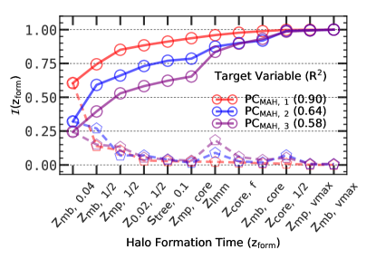
Figure 3: Performances ($R^{2}$) and contributions ($\mathcal{I}$) using formation times to predict the first three ${\rm PC}_{\rm MAH}$s based on RF regressors (see Appendix A.2 for the RF model). Dashed: importance values $\mathcal{I}$ of predictors. Solid: the cumulative of $\mathcal{I}$. The overall performances, $R^{2}$, are shown in the parentheses in the legend. Halos are taken from the mass-limited sample $\rm S_{c}^{\prime}$ with $M_{\rm halo}\geq 5\times 10^{11}\,h^{-1}{\rm M_{\odot}}$ (see §2.1 and Table 1).

In Appendix B we list the formation times we use and their detailed definitions. Because of the large number of formation times and the potential nonlinear pattern in their relations with PCs, RF is an ideal tool for this task. In Appendix A.2 we describe the RF algorithm in detail. The two important outputs from the RF analysis are (1) the fraction of explained variance, $R^{2}$, and (2) the feature importance, $\mathcal{I}(x)$, for any predictor variable $x$. These two quantities measure the performance of the regression and the contribution from each predictor variable in explaining the target variable, respectively. Figure 3 shows how different formation times contribute to the diversity of the halo MAH. Here we use sample $\rm S_{c}^{\prime}$ in which all of the formation times are well defined, as described in the §2.1 (see also Table 1), to regress the first three MAH PCs on all of the formation times. The performance, $R^{2}$, and the contribution $\mathcal{I}(x)$ of each formation time $x$ to each PC are plotted. For all PCs, the contribution from $z_{{\rm mb},0.04}$ is the most dominant, while $z_{{\rm mb},1/2}$ is also significant. However, the importance of both decreases in higher order PCs. Interestingly, the last major merger redshift, $z_{\rm lmm}$, which contributes little to ${\rm PC}_{\rm MAH,1}$, is increasingly important as the PC order increases. For ${\rm PC}_{\rm MAH,3}$, the contribution from $z_{\rm lmm}$ is comparable to those from the other two formation times, $z_{{\rm mb},0.04}$, and $z_{{\rm mb},1/2}$. Since mathematically higher order PCs are capable of capturing more subtle patterns in the feature space, this behavior of the importance curves means that assembly variables, such as $z_{{\rm mb},0.04}$, and $z_{{\rm mb},1/2}$, mainly describe the low-order, overall patterns of the halo assembly history, while major mergers are an important factor in producing the fine structure in MAHs.

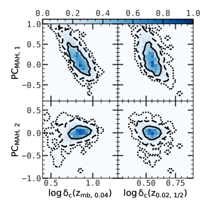
Figure 4: Relation of halo formation time $z_{{\rm mb},\ 0.04}$ (left) or $z_{{\rm 0.02},\ 1/2}$ (right) to the first two MAH PCs. Solid, dashed, and dotted contours cover 1, 2, 3 $\sigma$ regions, respectively. Normalized 2D histograms are color-coded according to the color bar. Halos are taken from the mass-limited sample $\rm S_{c}^{\prime}$ with $M_{\rm halo}\geq 5\times 10^{11}\,h^{-1}{\rm M_{\odot}}$ (see §2.1 and Table 1).

The contribution curves in Figure 3 automatically suppress variable competition where multiple degenerate feature variables compete in the prediction contribution to the target variable. In the RF, if two variables compete but one of them is slightly better, then the split algorithm prefers the better one and gives it a higher importance value $\mathcal{I}(x)$. To show this more clearly, Figure 4 plots the correlations between $z_{{\rm mb},0.04}$, $z_{0.02,1/2}$ and the first two MAH PCs. Strong and nearly linear correlation between ${\rm PC}_{\rm MAH,1}$ and $z_{{\rm mb},0.04}$, and between ${\rm PC}_{{\rm MAH},1}$ and $z_{0.02,1/2}$ are seen, indicating that the variances in both two formation times contribute significantly to the variance in the MAH of the halos. Inspecting the contours, one can also see that the correlation between ${\rm PC}_{\rm MAH,1}$ and $z_{{\rm mb},0.04}$ appears stronger. The larger contribution value to ${\rm PC}_{{\rm MAH},1}$ from $z_{{\rm mb},0.04}$ than from $z_{0.02,1/2}$ shown in Figure 3 validates the strength of the correlation.

Figure 4 also demonstrates that the description provided by a single halo formation time is incomplete. The large scatter seen in the contours of $\rm PC_{MAH,1}$ versus formation times means that the direction of the largest scatter in the MAH space is not fully aligned with the scatter caused by formation time, and that other parameters must also contribute to the distribution of halos in the MAH space. Moreover, compared to ${\rm PC}_{{\rm MAH},1}$, ${\rm PC}_{{\rm MAH},2}$ has much weaker correlation with the halo formation times. Thus, the information contained in the second PC of MAH, which contributes $10\%$-$20\%$ to the total variance as seen from the upper panel of Figure 1, is almost entirely missed when a single formation time is used to predict the MAH.

The degeneracy and completeness problems can, in principle, be overcome if we use PCs to describe the assembly history, as PCs are linearly independent of each other. Typically, the use of a small number of low-order PCs can solve most of the problems associated with the regression of halo MAHs. If more subtle information is needed, one can always add more PCs without introducing too much degeneracy into the problem.

4 Relating Halo Structure to Assembly History and Environment

In this section, we investigate how halo structural properties are related to halo assembly history and environment. First, we will examine which of the assembly history indicators correlates the best with halo structural properties. Second, we will show to what extent the halo structure can be explained by assembly history and environment, and we answer the question whether there is a single dominating predictor for halo structure or if the predictors are degenerate in predicting halo structure. Third, we will show that our conclusion is valid even when halo mass is fixed. Finally, we revisit the problem of assembly bias, aiming to identify environment-assembly pairs of strong correlation.

4.1 Halo Structure versus Assembly History

It is well known that halo concentration is correlated with halo MAH (see e.g., Navarro et al., 1997; Jing, 2000; Wechsler et al., 2002; MacCiò et al., 2008; Zhao et al., 2003a, b, 2009). However, it is still unclear which single assembly parameter best predicts the concentration, and whether combinations of multiple parameters can improve the prediction precision. The same problem exists when we consider other halo structural properties, for example, the axis ratio $q_{\rm axis}$ and the spin parameter $\lambda_{\rm s}$.

The difficulties involved here arise from the high dimension of the feature space, the degeneracy or correlation among predictors, a possible nonlinear effect from predictors to target, and the “bias-variance” trade-off in choosing model complexity. Again, Random Forest can be used to tackle these problems (see Appendix A.2). To this end, we build the regressor $y={\rm RF}(\mathrm{{\bf x}})$, where $y$ is one of the three structural properties: $c$, $q_{\rm axis}$ or $\lambda_{\rm s}$, and $\mathrm{{\bf x}}$ are halo assembly indicators, either the first 10 MAH PCs, or all formation times. We also include halo mass in the predictor variables, because it is treated as one of the major parameters in many halo-related problems. All these regressors are built based on sample $\rm S_{c}^{\prime}$ (see §2.1 and Table 1) in which all formation times are well defined for all halos.

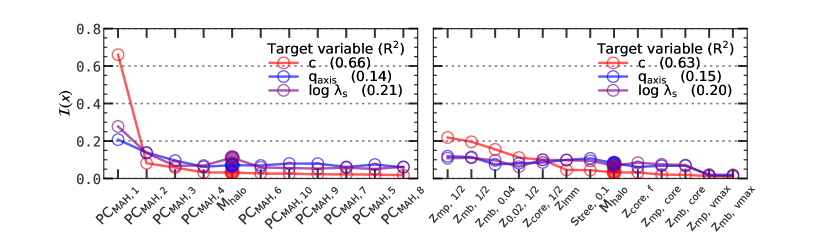
Figure 5: Contributions $\mathcal{I}(x)$ in regressing halo concentration $c$ (red), shape parameter $q_{\rm axis}$ (blue), or spin parameter $\log\lambda_{\rm s}$ (purple) on halo assembly history variables: the first 10 PCs of MAH (left panel) or formation times (right panel). Halo mass is also included as a predictor variable and is represented by filled symbols. For each case, $R^{2}$ indicates the overall performance of the regression. Halos are taken from the mass-limited sample $\rm S_{c}^{\prime}$ with $M_{\rm halo}\geq 5\times 10^{11}\,h^{-1}{\rm M_{\odot}}$ (see §2.1 and Table 1).

The outputs of RF regressions, including the performance, $R^{2}$, and the contribution $\mathcal{I}(x)$ from each predictor variable, are shown in Figure 5. As one can see from the red curves, when a large number of predictors are used, the upper limit in the prediction of $c$ using assembly history is about $65\%$. This indicates that the concentration parameter $c$ of a halo is largely determined by its assembly history. About $35\%$ of the variance is still missing if one uses only the mean relation to predict $c$ from assembly history. Furthermore, as seen from the left panel, the first MAH PC is by far the most important, accounting for about $67\%$ of the total information provided by the MAH. As a comparison, in the right panel, the combination of the three formation times, $z_{{\rm mb},1/2}$, $z_{{\rm mp},1/2}$ and $z_{{\rm mb},0.04}$, contains about the same amount of information as ${\rm PC}_{\rm MAH,1}$. Thus, if a single parameter is to be adopted as the predictor of $c$, ${\rm PC}_{\rm MAH,1}$ is the preferred choice. We have also tried to combine halo formation times and PCs of the MAH as predictors, and we found that the overall performance changes little, indicating that the MAH PCs dominate the information content about halo concentration.

For $q_{\rm axis}$ and $\lambda_{\rm s}$, the upper-limit performances $R^{2}$, achieved by either PCs or formation times, are about $15\%$ and $20\%$, respectively, much worse than $c$. No single variable seems to dominate the contribution, as indicated by the long and low tail in the $\mathcal{I}(x)$ plot. These suggest that the axis ratio and spin can be affected by many factors related to halo mass assembly, but the effects are all small. The similarity in behavior between $\lambda_{\rm s}$ and $q_{\rm axis}$ suggests that these two quantities may share parts of their origins. Indeed, as we will show below (§4.2), $\lambda_{\rm s}$ and $q_{\rm axis}$ are strongly correlated, and both show strong correlation with the anisotropy of the local tidal field.

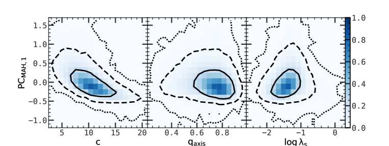
Figure 6: Relation of halo concentration $c$ (left), shape parameter $q_{\rm axis}$ (central), or the spin parameter $\log\lambda_{\rm s}$ (right) and the first PC of the halo MAH. In each panel, the solid, dashed, and dotted contours cover the 1, 2, and 3$\sigma$ regions, respectively. The normalized 2D histograms are color-coded according to the color bar. Halos are taken from the mass-limited sample $\rm S_{c}^{\prime}$ with $M_{\rm halo}\geq 5\times 10^{11}\,h^{-1}{\rm M_{\odot}}$ (see §2.1 and Table 1).

Figure 6 shows the distribution of halos in the $\rm PC_{MAH,1}$ - structural parameter space. There is a strong trend that halos assembled late (large ${\rm PC}_{\rm MAH,1}$) tend to be less concentrated, and a weak trend that such halos tend to be more elongated and spin faster. These are all consistent with the output from the RF regressors and verify that the small contributions from assembly indicators to $\lambda_{\rm s}$ and $q_{\rm axis}$ are produced by the large scatter, rather than by variable competitions.

4.2 Environmental Effect and Spin-Shape Interaction

We now add environmental predictors to the regression of the structural properties. To quantify the effects of variable competition, we adopt a commonly used approach called “growing”, where a series of regressors is built up with increasing number of predictors. (The approach is called “pruning”, if the series runs reversely). Whenever there is a tight correlation between an added predictor and the predictors already used, competition will show up as changes in their importance values, $\mathcal{I}(x)$, but the overall performance, $R^{2}$, will not be changed significantly by the addition.

As demonstrated in §4.1, among all halo assembly indicators, the first PC of the halo MAH is the dominating indicator for $c$. Even for $q_{\rm axis}$ and $\lambda_{\rm s}$, it is still the most important although less dominating. We therefore start by building a Random Forest regressor $y={\rm RF}_{1}({\rm PC_{MAH,1}},M_{\rm halo})$, where $y$ is one of the three structural quantities. Again, the inclusion of $M_{\rm halo}$ is motivated by the fact that halo mass is traditionally considered as one of the most important quantities distinguishing halos. We also calculate the performance $R_{1}^{2}$ as well as the contributions $\mathcal{I}_{1}(x)$ of the regressor. We then add the two environmental quantities, the bias factor $b$ and the tidal anisotropy $\alpha_{\mathcal{T}}$, to build a second regressor, $y={\rm RF}_{2}({\rm PC_{MAH,1}},M_{\rm halo},b,\alpha_{\mathcal{T}})$, and obtain the corresponding $R_{2}^{2}$ and $\mathcal{I}_{2}(x)$.

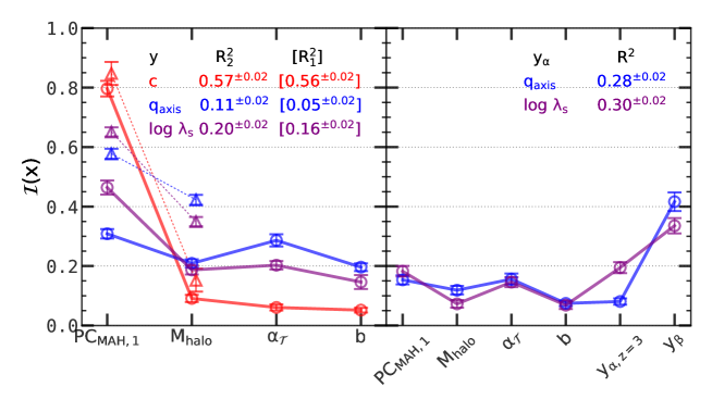
Figure 7: Left: contributions $\mathcal{I}(x)$ from various predictors $x$ to halo structural quantities $y$: concentration $c$ (red), shape parameter $q_{\rm axis}$ (blue), or the spin parameter $\log\lambda_{\rm s}$ (purple). Solid lines connecting circles show the results when using the first MAH PC $\rm PC_{MAH,1}$, halo mass $M_{\rm halo}$, tidal anisotropy $\alpha_{\mathcal{T}}$ and bias factor $b$ as predictors. Dashed lines connecting triangles show the results when using only $\rm PC_{MAH,1}$ and $M_{\rm halo}$. The overall performances $R_{2}^{2}$ (with environment) and $R_{1}^{2}$ (without environment) are also indicated in the panel. Right: similar to the left panel, except that we add the initial condition of each structural property at redshift $z=3$ and a $\beta$-structure parameter $y_{\beta}$ into the predictors. The target variable, now denoted as $y_{\alpha}$, is either the shape parameter $q_{\rm axis}$ (blue) or the spin parameter $\log\lambda_{\rm s}$ (purple). For $q_{\rm axis}$, the $y_{\beta}$ is $\log\lambda_{\rm s}$, and for $\log\lambda_{\rm s}$, the $y_{\beta}$ is $q_{\rm axis}$. The overall performance $R^{2}$ is also indicated in the panel. In both panels, halos are taken from the mass-limited sample $\rm S_{c}^{\prime}$ with $M_{\rm halo}\geq 5\times 10^{11}\,h^{-1}{\rm M_{\odot}}$ (see §2.1 and Table 1). The error bars are calculated using 100 half-size resamplings without replacement.

The left panel of Figure 7 shows the contribution, $\mathcal{I}(x)$, of these two regressors for each of the three structure properties described above, with the values of $R^{2}$ indicated, using sample $\rm S_{c}^{\prime}$ (see §2.1 and Table 1). To estimate the uncertainty in the results, we generate 100 random subsamples, each consisting of half of the halos randomly selected from the original sample $\rm S_{c}^{\prime}$ without replacement. The errors of $R^{2}$ and $\mathcal{I}(x)$ are then estimated as the standard deviations among these subsamples. The reason why we do not use the standard bootstrap technique is that the sampling with replacement will lead to an artificially large $R^{2}$ in the Random Forest regressor, because the repeated data points may appear both in the training set that shapes the decision trees and the out-of-bag (OOB) set (see Appendix A.2) that is used to test the performance, making the performance overestimated.

In the case of $c$, the inclusion of environment only increases $R^{2}$ from $0.56$ to $0.57$, and the importance value $\mathcal{I}(x_{\rm env})$ is below $0.1$. These two results indicate that environment has little impact on halo concentration $c$, that the concentration $c$ is well determined by the first PC of the MAH, and that the weak dependence of $c$ on environment is mainly through the dependence of halo assembly on environment (assembly bias). These are consistent with the finding of Lu et al. (2006) that the density profiles of individual halos can be modeled accurately from their MAHs. These are also consistent with the result obtained with the Gaussian process regression by Han et al. (2019), who found that the dependence of halo bias on halo concentration is mainly through the dependence of the bias on formation time.

For $q_{\rm axis}$, the $R^{2}$ is doubled, from $0.05$ to $0.11$, when environment factors are included. From the importance curve, $\mathcal{I}(x)$, one can see that these environment factors take away about half of the contribution from the halo mass and $\rm PC_{MAH,1}$. These results together suggest that environment can affect halo shape significantly and is at least as important as halo mass and the PCs of the MAH.

For the spin parameter, the value of $R^{2}$ increases from $0.16$ to $0.20$ when environment factors are included. The increase, $0.04$, is about $20\%$, suggesting that these environment factors do have a sizable effect on halo spin. The contribution, $\mathcal{I}(b)+\mathcal{I}(\alpha_{\mathcal{T}})=35\%$, is larger than the $20\%$ they contribute to $R^{2}$, suggesting that some of the contribution is actually taken from the halo assembly history and halo mass. Thus, when interpreting the dependence of halo spin on environment, one should remember that part of it may actually come from its degeneracy with halo assembly history.

Another difference between $c$ and the other two structural parameters is in their values of $R^{2}$. Both $q_{\rm axis}$ and $\log\lambda_{\rm s}$ have fairly small $R^{2}$, much smaller than $50\%$. This indicates that the major contributors to these two structural parameters are not yet found. In general, factors that can affect halo structural properties can be classified into three categories: the initial conditions of halos, the intrinsic properties of halos (e.g., $M_{\rm halo}$, $\rm PC_{MAH,1}$), and halo environment (e.g., $\alpha_{\mathcal{T}}$ and $b$). The interaction of halos with their environment depends not only on the environment, but also on halo properties. For example, because a halo is coupled to the local tidal torque only through its quadrupole, we expect that the spin and shape of a halo are correlated. Motivated by this and the similar behavior of the shape and spin parameters revealed in §4.1, we add the spin parameter into the predictors of the shape, and vice versa. We denote the target structure parameter as $y_{\alpha}$ and the added structure parameter $y_{\beta}$. In addition, we also consider the “initial condition” of a halo by tracing all of the halo particles back to redshift $z=3$ and using these particles to calculate the corresponding shape and spin parameters. This quantity for $y_{\alpha}$, denoted by $y_{\alpha,z=3}$, is also added into the set of predictors. The right panel of Figure 7 shows the result when this set of variables are used to predict halo structures. Among all the predictor variables, $y_{\beta}$ is the most important for $y_{\alpha}$, indicating that $q_{\rm axis}$ and $\log\lambda_{\rm s}$ are strongly correlated. For $\lambda_{\rm s}$, its initial value also matters, ranked as the second important predictor. The performance, $R^{2}$, for both $\lambda_{\rm s}$ and $q_{\rm axis}$ is now boosted significantly, to $\sim 0.3$. However, even in this case, $R^{2}$ is still less than $50\%$, meaning that the causes of the main parts of the variances in both $\lambda_{\rm s}$ and $q_{\rm axis}$ are still to be identified. This also indicates that, unlike the concentration parameter $c$, which is determined largely by halo assembly, $\lambda_{\rm s}$ and $q_{\rm axis}$ may depend on the details of the initial conditions, assembly, and environment. Morinaga & Ishiyama (2020) provided a possible scenario where accretion from filaments may partly account for halo shape and orientation. However, the large scatter and weak trend in their results indicate that the driving factor of halo shape and orientation is still missing. All these suggest that many nuanced factors can contribute to the variances of $\lambda_{\rm s}$ and $q_{\rm axis}$. Models for distributions of $\lambda_{\rm s}$ and $q_{\rm axis}$ have to take into account these nuances by assuming some random processes, such as a normal or log-normal process according to the central-limit theorem.

4.3 Dependence on Halo Mass

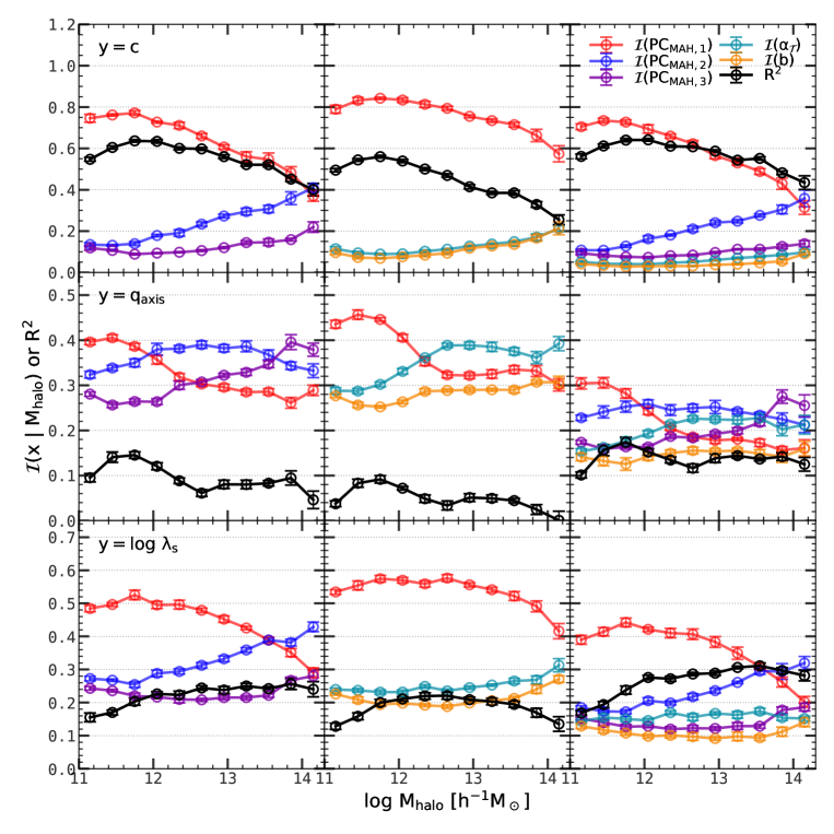
Figure 8: Contributions $\mathcal{I}(x)$ from different predictor variables $x$ to the halo structural properties $y$ for halos of different masses. The upper, central, and bottom rows show the results for structural properties $y=c$, $q_{\rm axis}$ and $\log\lambda_{\rm s}$, respectively. The left, middle, and right columns show the regressors built with predictor variables $\mathrm{{\bf x}}=({\rm PC_{MAH,1}},{\rm PC_{MAH,2}},{\rm PC_{MAH,3}})$, $({\rm PC_{MAH,1}},\alpha_{\cal T},b)$, and $({\rm PC_{MAH,1}},{\rm PC_{MAH,2}},{\rm PC_{MAH,3}},\alpha_{\cal T},b)$, respectively. Contributions from different predictor variables $x$ are shown with different colors, as indicated in the upper right panel. The overall performance $R^{2}$ for each regressor is represented by the black symbols. The error bars are obtained by 10 half-size resamplings without replacement. Halos are those in the large sample $\rm S_{L}$ (see §2.1 and Table 1).

The regressors for halo structure (presented in §4.1 and §4.2) are all built using the mass-limited sample. The model training processes and performance measurements are thus dominated by low-mass halos, which are more abundant. However, halos with different masses may have different properties. For example, the halo assembly bias, as reflected by the correlation between halo formation time and the bias factor, is found to be significant only for low-mass halos (e.g., Gao et al., 2005; Gao & White, 2007; Li et al., 2008). It is, therefore, interesting to see how the structural properties of massive halos depend on assembly and environment, and how environmental and assembly effects on these halos are related to each other.

Here we quantify such a halo mass dependence by building RF regressors for subsamples of a given halo mass, using the large sample $\rm S_{L}$ (see §2.1 and Table 1). For halos with given mass, $M_{\rm halo}$, and for each of the three structural properties, $y=c$, $q_{\rm axis}$ and $\log\lambda_{\rm s}$, we build three forest regressors $y={\rm RF}(\mathrm{{\bf x}}|M_{\rm halo})$ with different sets of predictor variables $\mathrm{{\bf x}}$:

• $\mathrm{{\bf x}}=({\rm PC_{MAH,1}},\,{\rm PC_{MAH,2}},\,{\rm PC_{MAH,3}})$, the first three PCs of the halo MAH;

• $\mathrm{{\bf x}}=({\rm PC_{MAH,1}},\,\alpha_{\cal T},b)$, the first PC of the halo MAH and environmental parameters;

• $\mathrm{{\bf x}}=({\rm PC_{MAH,1}},\,{\rm PC_{MAH,2}},\,{\rm PC_{MAH,3}},\,\alpha_{\cal T},\,b)$, the first three PCs of the MAH plus the environmental parameters.

The reason for including ${\rm PC_{MAH,2}}$ and ${\rm PC_{MAH,3}}$ is that the MAHs of massive halos may be more complicated than low-mass ones, and high-order PCs may be needed to capture the more subtle components in their MAHs.

Figure 8 shows the contribution curves and performances of regressors $y={\rm RF}(\mathrm{{\bf x}}|M_{\rm halo})$ for different halo structural properties, $y$, using different predictor variables, $\mathrm{{\bf x}}$, and for halos of different masses. In the case where $\mathrm{{\bf x}}$ is the first three MAH PCs (panels in the left column), the $\rm PC_{MAH,1}$ is always the most important for the structures of low-mass halos. However, as the halo mass increases, the importance of $\rm PC_{MAH,1}$ decreases and eventually is taken over by higher order PCs (the second or the third). Massive halos may have more diverse accretion histories (see, e.g., Obreschkow et al., 2020, who found that tree entropy increases with halo mass), so their structural properties may also be more complex. By using higher order PCs, the complex formation history can be captured so that a better prediction for halo structure properties can be achieved.

As discussed in §4.2, for the total halo population, environmental effects are different for the three halo structural properties. Similar conclusions can be reached for halos of a given mass. The middle and right columns in Figure 8 show results for regressors that combine the MAH and environment as predictors. For the halo concentration, the PCs of MAH always outperform environmental quantities, although there is a slight increase in $\mathcal{I}(x)$ for environment quantities at the high-mass end. Compared to the regressor with only MAH PCs (upper left panel), the performance $R^{2}$ including the two environmental properties (upper right panel) only increases slightly, indicating again that the environmental effect on halo concentration is mainly through the dependence of halo MAH on environment.

The environmental effect on the shape parameter, $q_{\rm axis}$, is totally different. As seen from the contribution curves, the environment is as important as MAH, and including the environment variables increases $R^{2}$ significantly. This implies that the environmental effect on the halo shape parameter is important, and that the effect is not degenerate with that of the MAH. The environmental contribution to the spin parameter, $\lambda_{\rm s}$, is intermediate, larger than that to the concentration parameter but smaller than that to the shape parameter. The value of $R^{2}$ after including environment variables increases, but less significantly than in the case of the shape parameter. This suggests that the environmental effect does contribute to halo spins, but part of the contribution is taken from the assembly.

4.4 Halo Assembly Bias

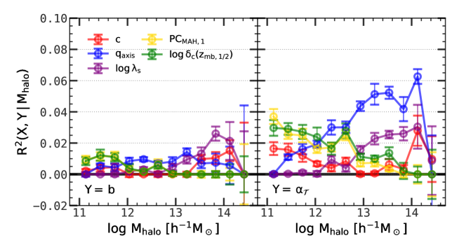
Figure 9: Random Forest regression performance $R^{2}(X,Y|M_{\rm halo})$ of pairs of variables $(X,\,Y)$ for halos with a given mass, where $Y$ is an environmental quantity (left panel: halo bias factor $b$; right panel: tidal anisotropy parameter $\alpha_{\mathcal{T}}$), and $X$ is either a structural quantity or an assembly history quantity, as represented with different colors. The error bars of $R^{2}$ are obtained by 10 half-size resamplings without replacement. Halos are taken from the large sample $\rm S_{L}$ (see §2.1 and Table 1).

As a final demonstration of the application of the Random Forest regressor, we show how assembly parameters correlate with environment for halos of a given mass. Such a correlation is usually referred to as the halo assembly bias. The purpose here is to identify the best correlated pair of variables $(X,\,Y)$ at given halo mass, where $X$ is an assembly property and $Y$ is an environmental property. The method to measure the correlation strength is straightforward. First, we bin halos in sample $\rm S_{L}$ (see §2.1 and Table 1) into subsamples according to the halo mass. Within each subsample, we build a Random Forest regressor for each pair of variables $(X,\,Y)$. The value of $R^{2}(X,Y|M_{\rm halo})$ then provides a measurement of the correlation strength between the two quantities. Figure 9 shows the results for different cases, where the environmental quantity $Y$ is either the bias factor $b$ or the tidal anisotropy parameter $\alpha_{\mathcal{T}}$, and $X$ is either $\rm PC_{MAH,1}$ or $\log\delta_{\rm c}(z_{{\rm mb},1/2})$. As one can see, the dependence of $\log\delta_{\rm c}(z_{{\rm mb},1/2})$ on $b$ is present only for halos with $M_{\rm halo}<10^{13}h^{-1}{\rm M}_{\odot}$, and totally absent for more massive ones. The values of $R^{2}$ between $b$ and the two assembly properties are both smaller than $2\%$, indicating that the correlation between $b$ and assembly history is weak. These results are consistent with those obtained previously (e.g., Gao et al., 2005; Gao & White, 2007; Li et al., 2008): the assembly bias is significant only for low-mass halos, and one has to average over a large number of halos to detect the weak trend.

For comparison, we also build regressors between structure properties ($c$, $\lambda_{\rm s}$ and $q_{\rm axis}$) and $b$ for halos of a given mass. The results are shown in the left panel of Figure 9. Clearly, the dependence of these properties on $b$ is also weak. The results are consistent with those obtained previously by Mao et al. (2018), who found that $b$ is better correlated with $c$ and $\lambda_{\rm s}$ than with assembly properties for massive halos.

In a recent paper, Ramakrishnan et al. (2019) showed that the tidal anisotropy parameter, $\alpha_{\mathcal{T}}$, is a good variable that correlates well with many structural properties. We present the correlation between $\alpha_{\mathcal{T}}$ and other halo quantities in the right panel of Figure 9. It is clear that $\alpha_{\mathcal{T}}$ shows a better correlation with halo intrinsic properties than the bias factor, as indicated by the larger values of $R^{2}$. In particular, the correlations between the assembly properties ($\delta_{\rm c}(z_{\rm mb,1/2})$ and $PC_{\rm MAH,1}$) and $\alpha_{\mathcal{T}}$ are significant, except at the very massive end. In §4.2, we demonstrate that part of the contribution from the environment to the structural properties is produced by the degeneracy between the environment and the halo assembly history. The strong relation between $\alpha_{\mathcal{T}}$ and assembly history is a proof of this degeneracy. Note that $q_{\rm axis}$ shows a strong correlation with $\alpha_{\mathcal{T}}$ for massive halos, indicating that the local tidal field plays an important role in determining the shape of the halo.

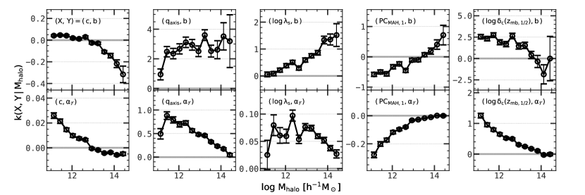
Figure 10: Linear regression slope $k(X,Y|M_{\rm halo})$ of pairs of variables $(X,\,Y)$ for halos with a given mass, where $Y$ is an environmental quantity and $X$ is either a structural quantity or an assembly history quantity. Each panel is for a pair of $(X,\,Y)$. The error bars are standard errors estimated from linear regression model. Halos are taken from the large sample $\rm S_{L}$ (see §2.1 and Table 1).

As mentioned above, the small values of $R^{2}$ between assembly and environment imply that assembly bias is a weak relation compared to the variance. Detecting such a bias thus needs the average over a large number of halos. To obtain the mean trend in the bias relation, we can build linear regression models between pairs of variables and use the slopes of the regression, $k$, to represent the mean trend between the two variables in question. Figure 10 shows the slopes of halo properties with $b$ and $\alpha_{\cal T}$ for halos with different masses. Given any two variables, a larger absolute value of $k$ means a more significant linear correlation of the two variables for halos of a given mass. The relations between halo environment and different halo properties show different trends with halo mass. For example, the slope $k(\log\delta_{\rm c}(z_{{\rm mb},1/2}),b|M_{\rm halo})$ is significant only at the low-mass end, while $k({\rm PC_{MAH,1}},b|M_{\rm halo})$ is significant at the low-mass end and becomes less significant at the high-mass end, suggesting that halo assembly bias is more important for halos of lower mass. In contrast, the slopes $k(c,b|M_{\rm halo})$, $k(q_{\rm axis},b|M_{\rm halo})$ and $k(\log\lambda_{\rm s},b|M_{\rm halo})$ are all more significant at the high-mass end. As discussed in Wang et al. (2011), this halo mass dependence is a result of the competition between the environmental effect and the self-gravity of the halo. For example, a higher density environment not only provides more material for halos to accrete, but also is the location of a stronger tidal field that tends to suppress halo accretion. Depending on the halo mass, one of the two effects dominates. For example, for lower mass halos where self-gravity is weaker, the local tidal field may be more effective in making them more elongated and spin faster, and in preventing them from accreting new mass, so as to make their mass assembly earlier and concentration higher. This is indeed what can be seen from the lower panels of Figure 10. We note, however, that the physical units of the different curves in these panels are not the same, so that these curves cannot be compared directly with one another. Note also that a significant value of $k$ does not necessarily imply a significant $R^{2}$ in Figure 9, and vice versa, because a linear model may not represent faithfully the data of nonlinear relations. In addition, the value of $R^{2}$ depends not only on the value of $k$, but also on the absolute value of the variance in the regressed sample.

5 Summary and discussion

In this paper, we have used the ELUCID $N$-body simulation to relate the structural properties of dark matter halos to their assembly history and environment. Our analysis is based on the PCA and the RF regressor. Our main results and their implications can be summarized as follows.

First, PCA is a simple and yet effective tool for reducing the dimension of the halo MAH, and it is preferred over formation times in characterizing the halo MAH. It has the following three major advantages (see §3 and §4.1):

• PCs are complete and linearly independent. The first three PCs can already explain more than $80\%$ of the variance of the halo MAH, with a reconstruction error $<10\%$.

• The PCs of the MAH have clear physical meanings. The lower order PCs, such as the first PC, are tightly related to the (halo formation) times when a halo forms fixed fractions of its current mass, such as $z_{{\rm mb},1/2}$, $z_{{\rm mb},0.04}$, and so on. Higher order PCs, on the other hand, are related to more subtle events, such as the presence of major mergers.

• PCs are the best, among all assembly indicators, to explain halo structure. The first PC, among all assembly indicators, accounts for about $67\%$, $20\%$, and $28\%$ of the variance in halo concentration, shape parameter, and spin parameter, respectively.

Second, the dependence on assembly and environment is quite different for the three halo structural properties (see §4.2). About $60\%$, $10\%$, and $20\%$ of the variances in $c$, $q_{\rm axis}$, and $\lambda_{\rm s}$, respectively, can be explained by four predictors: $\rm PC_{MAH,1}$, $M_{\rm halo}$, $\alpha_{\cal T}$ and $b$. Halo concentration is dominated by the first PC of the MAH, with the contributions from other factors negligible. For $q_{\rm axis}$ and $\lambda_{\rm s}$, there is no single property of assembly that is dominating. The environment has significant effects on these two structural parameters, but its effect on $\lambda_{\rm s}$ is degenerate with the assembly history. The correlation between $q_{\rm axis}$ and $\lambda_{\rm s}$ is strong, indicating that these two quantities share some common origins. The initial condition is also important for $\lambda_{\rm s}$. However, putting all the factors together, we see that the values of $R^{2}$ are still smaller than $0.5$ for both $q_{\rm axis}$ and $\lambda_{\rm s}$, indicating that these two halo quantities may be affected by many subtle factors and thus are difficult to model.

Third, the structural properties depend mainly on the first PC of the MAH for low-mass halos, but have a significant dependence on higher order PCs for high-mass halos. The conclusions for the overall population still hold for halos of a given mass: environment has almost no effect on $c$ once the MAH is included; environment is more important for $q_{\rm axis}$ and $\lambda_{\rm s}$, although its effect on $\lambda_{\rm s}$ is partly degenerate with that of the MAH.

Fourth, the tidal anisotropy, $\alpha_{\cal T}$, has a stronger correlation with halo assembly and structure than the bias factor $b$ does. We see that $\alpha_{\cal T}$ is correlated with halo assembly history for all halos except the most massive ones, and it also shows a significant correlation with $q_{\rm axis}$, indicating that the local tidal field plays an important role in shaping a halo. However, all types of assembly bias tested here are weak compared to the variance in the relation, and averaging with a large sample is needed to detect them reliably .

For dimension-reduction tasks such as those for the halo MAH, one may also use nonlinear algorithms, such as the locally linear embedding (LLE; Roweis, 2000), and the spectral embedding (Belkin & Niyogi, 2003). The degrees of freedom of these manifold-learning techniques are higher than those of the linear algorithms, so that they are not stable for noise data. Indeed, we have tried implementing LLE in halo MAH, but we found that it does not outperform the PCA in terms of both the reconstruction error and the correlation with halo structural properties.

The correlation of structural properties with halo assembly and environment revealed by the RF analysis provides insights into the halo population in the cosmic density field. Since galaxies form and evolve in dark matter halos, understanding the formation, structure, and environment of dark matter halos is a crucial step in establishing the link between galaxies and halos. Empirical approaches, such as (sub)halo abundance matching (Mo et al., 1999; Vale & Ostriker, 2004; Guo et al., 2010), clustering matching (Guo et al., 2016), age matching (Hearin & Watson, 2013), conditional color-magnitude diagrams (Xu et al., 2018), halo occupation distributions (Jing et al., 1998; Berlind & Weinberg, 2002), conditional luminosity functions (Yang et al., 2003), and those based on star formation rate (Lu et al., 2014; Moster et al., 2018; Behroozi et al., 2019), all use halo properties to make predictions for the galaxy population. A key question in all of these models is which halo quantities should be used as the predictors of galaxies. Using too little information about the halo population will make the model too simple to capture the real effects of halos on galaxy formation; using too many halo properties may be unnecessary because of the degeneracy between them. Our results, therefore, provide a foundation for building galaxy formation models such as those listed above.

For readers who are interested in generating Monte Carlo samples of halos of different structural properties, including dependencies on assembly and environment properties, we provide both an online calculator and a programming interface at https://www.chenyangyao.com/publication/20/haloprops/.

Appendix A Methods of analysis

Throughout this work, we use two statistical methods to analyze halo properties. The PCA is used to reduce the complexity of quantities in high-dimensional space, and the EDT, also called the RF, is used to study correlations among different quantities. A brief description of the two methods is given below. For a more detailed description, see Pattern Recognition and Machine Learning by Bishop (2006). The programming interfaces and implementation can be found in scikit-learn.

A.1 Principal Component Analysis

PCA is an unsupervised, reduced linear Gaussian dimension-reduction method (Pearson, 1901; Hotelling, 1933). Consider a set of $\rm N$ vectors $\mathrm{{\bf X}}=(\mathrm{{\bf x}}_{1},\ ...,\ \mathrm{{\bf x}}_{\rm N})^{\rm T}$, each in an $\rm M$-d space, $V_{\rm M}$. The idea of the PCA is to find an $\rm M^{\prime}$-d subspace, $V_{\rm M^{\prime}}$ ($\rm M^{\prime}\leq M$), in which the projection of $\mathrm{{\bf X}}$,

$$\mathrm{{\bf X^{\prime}}}=\mathrm{{\bf X}}\mathrm{{\bf P}}$$ (A1)

has maximal variance, where $\mathrm{{\bf P}}$ is the projection operator. It can be shown that the problem to be solved is equivalent to solving the eigenvalue problem for the sample covariance matrix of $\mathrm{{\bf X}}$, defined as

$$\mathrm{{\bf S}}=\sum_{i=1}^{\rm N}(\mathrm{{\bf x}}_{i}-\overline{\mathrm{{\bf x}}})(\mathrm{{\bf x}}_{i}-\overline{\mathrm{{\bf x}}})^{\rm T},$$ (A2)

where $\overline{\mathrm{{\bf x}}}=\sum_{i=1}^{\rm N}\mathrm{{\bf x}}_{i}/{\rm N}$ is the sample mean. If we rank the eigenvalues in a descending order, the first eigenvector of $\mathrm{{\bf S}}$, $\mathrm{{\bf v}}_{1}$, is the direction along which the sample has the maximum projected variance, $\lambda_{1}=\mathrm{{\bf v}}_{1}^{\rm T}\mathrm{{\bf S}}\mathrm{{\bf v}}_{1}$. This variance is exactly the first eigenvalue of $\mathrm{{\bf S}}$. Similarly, the $i$th eigenvector and the $i$th eigenvalue are, respectively, the direction and value of the $i$th largest variance. Consider the space $V_{\rm M^{\prime}}$ spanned by the first $\rm M^{\prime}$ eigenvectors. The linearity of the transformation can be used to prove that the projected variance in ${\rm M}^{\prime}$ is $\sigma^{2}=\sum_{i=1}^{\rm M^{\prime}}\lambda_{i}$. Thus, one can project each data point $\mathrm{{\bf x}}$ into $V_{\rm M^{\prime}}$ by $\mathrm{{\bf P}}=(\mathrm{{\bf v}}_{1},\ ...,\ \mathrm{{\bf v}}_{\rm M^{\prime}})$: $\mathrm{{\bf x^{\prime}}}=\mathrm{{\bf P}}^{\rm T}\mathrm{{\bf x}}$, to find a lower-dimension representation for it. The $i$th component of $\mathrm{{\bf x^{\prime}}}$ is called the $i$th PC of this data point in the sample.

In general, any dimension-reduction algorithm will lose information contained in the original data. In PCA, the proportional variance explained (PVE) by the $i$th PC, defined as

$${\rm PVE}_{i}=\frac{\lambda_{i}}{{\rm Tr}(\mathrm{{\bf S}})},$$ (A3)

is used to quantify the importance of the $i$th PC. The cumulative PVE, defined as

$${\rm CPVE_{M^{\prime}}}=\sum_{i=1}^{\rm M^{\prime}}{\rm PVE}_{i},$$ (A4)

can be used to quantify the performance of using the first $\rm M^{\prime}$ PCs in the dimension reduction. Typically, if the data in question are generated from an intrinsic process of lower dimension, the CPVE should quickly converge to $1$ as $\rm M^{\prime}$ increases. We will see that halo assembly histories have this property (§3.1).

The inverse operation of the projection, $\tilde{\mathrm{{\bf x}}}=\mathrm{{\bf P}}\mathrm{{\bf x^{\prime}}}$, allows one to reconstruct the original vector, but with information loss. We use the following quantity,

$$e=\left\lVert\tilde{\mathrm{{\bf x}}}-\mathrm{{\bf x}}\right\rVert/\left\lVert\mathrm{{\bf x}}\right\rVert,$$ (A5)

to quantify the reconstruction error of the data point $\mathrm{{\bf x}}$.

A.2 The Random Forest

The RF regressor or classifier is a supervised, decision-tree-based, highly nonlinear, nonparametric model ensemble method in statistical learning (Breiman, 2001). Here we first introduce the decision tree algorithm, and then we discuss how the trees are combined into a forest to make a regression or classification.

Given a set of observations $D=\{(\mathrm{{\bf x}}_{i},y_{i})\}_{i=1}^{\rm N}$, each consisting of a vector of predictor variables $\mathrm{{\bf x}}_{i}\in\mathbb{R}^{\rm M}$, and a target random variable $y_{i}$ (continuous in the regression problem, discrete in the classification problem), a decision tree $\rm T$ can be trained to fit the data by minimizing some error functional $\mathcal{E}({\rm T}|D)$. In regression problems, a common choice for the error functional, which we adopt here, is the mean residual sum-of-square,

$$\mathcal{E({\rm T}|D)}={1\over{\rm N}}\sum_{n=1}^{\rm N}[f(\mathrm{{\bf x}}_{i})-y_{i}]^{2},$$ (A6)

where $f(\mathrm{{\bf x}}_{i})$ is the predicted value for the $i$th observation by the tree $\rm T$. The tree can then be used to predict the target value for a future test observation, $\mathrm{{\bf x}}$.

A decision tree is built by sequentially bipartitioning the feature space along some axes. At each partitioned region $\mathcal{R}$ in the feature space, the tree fits the observations by a constant function,

$$f(\mathrm{{\bf x}})={1\over{\rm N}_{\mathcal{R}}}\sum_{n=1}^{{\rm N}_{\mathcal{R}}}y_{i},$$ (A7)

where the summation is over all observations in the region $\mathcal{R}$, and ${\rm N}_{\mathcal{R}}$ is the number of training observations in this region. In the first step, the variable $x$ to be bipartitioned and the position of the partition plane are both chosen to minimize the error functional $\mathcal{E}({\rm T}|D)$. After a partition, the feature space is split into two subregions, each of which can be bipartitioned further to minimize the error functional. This recursive process partitions the feature space into a tree-like structure and is continued until some stop criterion (e.g. the maximum tree height, or the maximum number of tree nodes, or the minimum number of data points in individual leaf nodes, defined as the nodes at the top of the tree) is achieved.

Once a tree is built, the amount of error reduced by partitioning variable $x$ can be computed as

$$\mathcal{I}_{{\rm T}|D}(x)=C\sum_{n}{\rm N}_{n}\left(\mathcal{E}_{n}-{{\rm N}_{n_{\rm L}}\over{\rm N}_{n}}\mathcal{E}_{n_{\rm L}}-{{\rm N}_{n_{\rm R}}\over{\rm N}_{n}}\mathcal{E}_{n_{\rm R}}\right).$$ (A8)

Here the summation is over all tree nodes partitioned by variable $x$. $\mathcal{E}_{n}$ is the error functional computed at observations in the region represented by node $n$ before partition; $\mathcal{E}_{n_{\rm L}}$ and $\mathcal{E}_{n_{\rm R}}$ are the errors computed at the left and right child nodes of node $n$, respectively, after partition; and $N_{n}$, $N_{n_{\rm L}}$ and $N_{n_{\rm R}}$ are the number of observations in node $n$ and its two child nodes, respectively. The normalization factor $C$ is chosen so that the summation of $\mathcal{I}$ from all feature variables is one. So defined, the quantity $\mathcal{I}_{{\rm T}|D}(x)$ is the amount of contribution from variable $x$ in building the regressor and can therefore be viewed as the important value of the variable in explaining target $y$.

Such a tree model suffers from the overfitting problem: the more complicated the tree is, the less training error it will have. However, the tree will eventually be dominated by noise as its height increases. Many methods have been proposed to control such overfitting, for example, the cross-validation, bootstrap, and jackknife ensembles. Here we adopt the RF, an extension of the bootstrap ensemble, designed specifically to deal with overfitting in tree-like algorithms. The building of an RF involves two levels of randomness. First, one uses $n_{\rm re}$ bootstrap resamplings, and each is used to train a tree ${\rm T}_{i}\ (i=1,...,n_{\rm re})$. Second, when training each of the $n_{\rm re}$ trees, only a random subset (size $n_{\rm var}<{\rm M}$) of all $\rm M$ predictor variables is used at each partition step. The $n_{\rm re}$ trees are then combined, and the final prediction for a given feature $\mathrm{{\bf x}}$, denoted as ${\rm RF}(\mathrm{{\bf x}})$, is then averaged among all trees (arithmetic average in regression, and majority voting in classification). Also, the importance of the predictor, $\mathcal{I}_{{\rm T}|D}(x)$, is averaged among trees, which we denote as $\mathcal{I}_{{\rm RF}|D}(x)$. The overall performance of the RF is represented by the explained variance fraction, $R^{2}$, defined as

$$R^{2}=1-\frac{\sum_{n=1}^{\rm N_{T}}[y_{n}-{\rm RF}(\mathrm{{\bf x_{n}}})]^{2}}{\sum_{n=1}^{\rm N_{T}}[y_{n}-\overline{y}]^{2}},$$ (A9)

where in principle the summation should be computed over an independent test sample, $\rm T$, of size $\rm N_{T}$. The RF regressor has the advantage that the test performance can be directly estimated with the OOB sample in the bootstrap process, and therefore an extra test sample is not necessary. In addition, RF does not suffer from the issue of scaling or arbitrary transformation of predictors, which exists in many nonlinear approaches, such as K-nearest-neighbors (KNNs) and support vector machines (SVMs).

The RF method has some free parameters to be specified, and we choose them based on the following considerations: (1) The number of trees in the forest, $n_{\rm re}$, should be as large as possible to suppress overfitting. But a larger $n_{\rm re}$ is computationally more difficult. In our analysis, we choose $n_{\rm re}=100$, which is sufficiently large for most applications of RF. (2) The number of predictors randomly chosen in the partition, $n_{\rm var}$, also controls the suppression of overfitting. We optimize the value of $n_{\rm var}$ by maximizing the OOB score through grid searching. (3) The tree termination criterion affects the complexity of each tree. We choose to control the number of data points in the leaf nodes, $s_{\rm leaf}$. This choice makes the tree self-adaptive when more data points are available, and also reduces issues associated with transformations of target variables and the choice of the error functional. The value of $s_{\rm leaf}$ is also optimized by maximizing the OOB score, again through grid searching.

Appendix B Definitions of Halo Formation Times

Because of the diversity in MAHs, different formation times can be defined to describe different aspects of the assembly. Here we summarize the halo formation times we used in our analysis. Most of the definitions can be found in Li et al. (2008), but we also add some new definitions that have been used by others. Since the halo mass and redshift in different time steps are discrete, the mass-redshift relation is linearly interpolated within adjacent time steps.

• $z_{{\rm mb},1/2}$: the highest redshift at which the main branch has assembled half of its final mass $M_{\rm halo}$ (e.g., van den Bosch, 2002; Shi et al., 2018).

• $z_{\rm mb,core}$: the highest redshift at which the main branch has reached a fixed mass $M_{\rm h,\ core}=10^{11.5}\,h^{-1}{\rm M_{\odot}}$. A halo at such a mass typically has the highest star formation efficiency (Van Den Bosch et al., 2003; Yang et al., 2003), and therefore is capable of forming a bright galaxy in it.

• $z_{{\rm mb},0.04}$: this is the highest redshift at which the main branch of a halo assembled $4\%$ of its final mass. This formation time is found to be related to the concentration of the halo in a wide range of cosmological models (see Zhao et al., 2009).

• $z_{{\rm mp},1/2}$: similar to $z_{{\rm mb},\ 1/2}$, but using the most massive progenitors (MMPs) in the entire tree rooted from a halo, instead of the main branch. This definition is used in Wang et al. (2011).

• $z_{\rm mp,core}$: similar to $z_{\rm mb,\ core}$, but using MMPs.

• $z_{{\rm 0.02},1/2}$: the highest redshift at which half of the halo mass has been assembled into its progenitors with masses $\geq 2\%$ of the halo mass. This definition is used in Navarro et al. (1997) to study the correlation between halo concentration and formation history (see also Jeeson-Daniel et al. (2011), where a different mass threshold is used).

• $z_{{\rm core},1/2}$: the highest redshift at which half of the halo mass has been assembled into its progenitors with masses $M_{\rm halo}\geq M_{\rm h,\ core}=10^{11.5}\,h^{-1}{\rm M_{\odot}}$. This represents the time when the massive progenitors are capable of forming large amounts of stars.

• $z_{{\rm core},f}$: the highest redshift at which a fraction $f=\frac{1}{2}(M_{\rm halo}/M_{\rm h,\ core})^{-\gamma}$ of the halo mass has been assembled into its progenitors with masses $M_{\rm halo}\geq M_{\rm h,\ core}$, where $\gamma=0.32$. This definition takes into account the dependence of star formation efficiency on halo mass (Yang et al., 2003).

• $z_{\rm mb,vmax}$: the redshift at which the main branch has achieved its maximum virial velocity. This definition, therefore, reflects the formation of the gravitational potential well.

• $z_{\rm mp,vmax}$: the same as $z_{\rm mb,\ vmax}$, but using the maximum virial velocity of MMPs.

• $z_{\rm lmm}$: the last major merger time of a halo. Here the major merger is defined as a merger event in which the mass ratio $r=m/M$ between the two merger parts is larger than one-third. A major merger is a violent event and may change the halo structure significantly.

• $s_{\rm tree,\beta}$: the tree entropy with entropy update efficiency $\beta$ (see Obreschkow et al., 2020). Different from the formation parameters defined above, this parameter is not associated with any specific event of the halo assembly history, but it describes the complexity of the whole tree. By construction, $s_{\rm tree,\beta}$ is bound to the range $[0,1]$. A close-to-zero $s_{\rm tree,\beta}$ represents a continuous accretion history, while a close-to-one $s_{\rm tree,\beta}$ describes a history that is given by the merger of two progenitors of equal mass. The parameter $\beta\in[0,\,1]$ controls the balance between the entropy inherited from the progenitors and that generated in recent merger events. We choose $\beta=0.1$ so that the tree entropy can reflect its assembly history at high $z$.

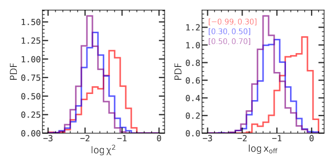
Figure 11: Distributions of halo relaxation-related parameters. Left: relaxation parameter $\chi^{2}_{\rm c}$, which is the normalized $\chi$-squared value in fitting the NFW profile. Right: offset parameter $x_{\rm off}$, which is the normalized distance from the center of mass to the most bound particle of the halo. In each panel, halos are taken from the mass-limited sample $\rm S_{c}^{\prime}$ with $M_{\rm halo}\geq 5\times 10^{11}\,h^{-1}{\rm M_{\odot}}$ (see §2.1 and Table 1), and are divided into three sub-samples according to their last major merger time $\log\,\delta_{\rm c}(z_{\rm lmm})$, indicated in the right panel with different colors.

Appendix C Effect of Unrelaxed Halos

As demonstrated by MacCiò et al. (2007), halos that have undergone recent major mergers may be unrelaxed and have structural properties significantly different from virialized halos (see also Ludlow et al., 2012). Following MacCiò et al. (2007) we define two parameters to quantify the dynamic states of halos. The first is the $\chi^{2}_{c}$ parameter, defined as the minimized $\chi^{2}$ in fitting the NFW profile, normalized by halo mass (see §2.3). The second is the offset parameter, $x_{\rm off}$, defined as the distance from the center of mass of the halo to the most bound particle, normalized by the virial radius. Figure 11 shows the distributions of $\chi^{2}_{\rm c}$ and $x_{\rm off}$ for subsamples with different last major merger times. As one can see, if a halo has experienced a recent major merger ($\log\,\delta_{\rm c}(z_{\rm lmm})<0.3$), it is likely that its profile deviates from the NFW profile, and that its most bound particle is far away from the center of mass of the halo.

Including those unrelaxed halos in our sample will significantly increase the variance of halo properties, thereby affecting the statistics derived from the sample. To reduce their effects, we exclude all halos that have undergone a major merger at $z<0.3$. This will remove $9.6\%$, $9.6\%$, $14.2\%$, $21.8\%$, $10.5\%$, and $13.8\%$ of halos in samples $\rm S_{1}$, $\rm S_{2}$, $\rm S_{3}$, $\rm S_{4}$, $\rm S_{c}$, and $\rm S_{L}$, respectively. To make our conclusion even less dependent on relaxation processes, we compute $\lambda_{\rm s}$ and $q_{\rm axis}$ using only simulated particles that are within a radius $2.5\,r_{\rm s}$ from the most bound particle, where $r_{\rm s}$ is the scale radius of the fitted NFW profile. According to our test, our results are not sensitive to the radius chosen.

References

- Behroozi et al. (2019) Behroozi, P., Wechsler, R. H., Hearin, A. P., & Conroy, C. 2019, Monthly Notices of the Royal Astronomical Society, 488, 3143, doi: 10.1093/mnras/stz1182
- Belkin & Niyogi (2003) Belkin, M., & Niyogi, P. 2003, Neural Computation, 15, 1373, doi: 10.1162/089976603321780317
- Berlind & Weinberg (2002) Berlind, A. A., & Weinberg, D. H. 2002, The Astrophysical Journal, 575, 587, doi: 10.1086/341469
- Bett et al. (2007) Bett, P., Eke, V., Frenk, C. S., et al. 2007, Monthly Notices of the Royal Astronomical Society, 376, 215, doi: 10.1111/j.1365-2966.2007.11432.x
- Bhattacharya et al. (2013) Bhattacharya, S., Habib, S., Heitmann, K., & Vikhlinin, A. 2013, The Astrophysical Journal, 766, 32, doi: 10.1088/0004-637X/766/1/32
- Bishop (2006) Bishop, C. M. 2006, Pattern Recognition and Machine Learning (Berlin: Springer)
- Bluck et al. (2019) Bluck, A. F. L., Maiolino, R., Sánchez, S. F., et al. 2019, Monthly Notices of the Royal Astronomical Society, 492, 96, doi: 10.1093/mnras/stz3264
- Bonjean et al. (2019) Bonjean, V., Aghanim, N., Salomé, P., et al. 2019, Astronomy & Astrophysics, 622, A137, doi: 10.1051/0004-6361/201833972
- Breiman (2001) Breiman, L. 2001, Machine Learning, 45, 5, doi: 10.1023/A:1010933404324
- Bryan & Norman (1998) Bryan, G. L., & Norman, M. L. 1998, The Astrophysical Journal, 495, 80, doi: 10.1086/305262
- Bullock et al. (2001) Bullock, J. S., Dekel, A., Kolatt, T. S., et al. 2001, The Astrophysical Journal, 555, 240, doi: 10.1086/321477
- Carroll et al. (1992) Carroll, S. M., Press, W. H., & Turner, E. L. 1992, Annual Review of Astronomy and Astrophysics, 30, 499, doi: 10.1146/annurev.aa.30.090192.002435
- Chen et al. (2019) Chen, Y., Mo, H. J., Li, C., et al. 2019, The Astrophysical Journal, 872, 180, doi: 10.3847/1538-4357/ab0208
- Cohn (2018) Cohn, J. D. 2018, Monthly Notices of the Royal Astronomical Society, 478, 2291, doi: 10.1093/mnras/sty1148
- Cohn & van de Voort (2015) Cohn, J. D., & van de Voort, F. 2015, Monthly Notices of the Royal Astronomical Society, 446, 3253, doi: 10.1093/mnras/stu2332
- Correa et al. (2015) Correa, C. A., Wyithe, J. S. B., Schaye, J., & Duffy, A. R. 2015, Monthly Notices of the Royal Astronomical Society, 450, 1514, doi: 10.1093/mnras/stv689
- Dalal et al. (2008) Dalal, N., White, M., Bond, J. R., & Shirokov, A. 2008, The Astrophysical Journal, 687, 12, doi: 10.1086/591512
- Davis et al. (1985) Davis, M., Efstathiou, G., Frenk, C. S., & White, S. D. M. 1985, The Astrophysical Journal, 292, 371, doi: 10.1086/163168
- de los Rios et al. (2016) de los Rios, M., Domínguez R., M. J., Paz, D., & Merchán, M. 2016, Monthly Notices of the Royal Astronomical Society, 458, 226, doi: 10.1093/mnras/stw215
- Desjacques (2008) Desjacques, V. 2008, Monthly Notices of the Royal Astronomical Society, 388, 638, doi: 10.1111/j.1365-2966.2008.13420.x
- Dobrycheva et al. (2017) Dobrycheva, D. V., Vavilova, I. B., Melnyk, O. V., & Elyiv, A. A. 2017, 1. https://arxiv.org/abs/1712.08955
- Dunkley et al. (2009) Dunkley, J., Komatsu, E., Nolta, M. R., et al. 2009, The Astrophysical Journal Supplement Series, 180, 306, doi: 10.1088/0067-0049/180/2/306
- Eisenstein & Hu (1998) Eisenstein, D. J., & Hu, W. 1998, The Astrophysical Journal, 496, 605, doi: 10.1086/305424
- Faltenbacher & White (2010) Faltenbacher, A., & White, S. D. M. 2010, The Astrophysical Journal, 708, 469, doi: 10.1088/0004-637X/708/1/469
- Gao et al. (2005) Gao, L., Springel, V., & White, S. D. M. 2005, Monthly Notices of the Royal Astronomical Society: Letters, 363, L66, doi: 10.1111/j.1745-3933.2005.00084.x
- Gao & White (2007) Gao, L., & White, S. D. M. 2007, Monthly Notices of the Royal Astronomical Society: Letters, 377, L5, doi: 10.1111/j.1745-3933.2007.00292.x
- Guo et al. (2016) Guo, H., Zheng, Z., Behroozi, P. S., et al. 2016, Monthly Notices of the Royal Astronomical Society, 459, 3040, doi: 10.1093/mnras/stw845
- Guo et al. (2010) Guo, Q., White, S., Li, C., & Boylan-Kolchin, M. 2010, Monthly Notices of the Royal Astronomical Society, 404, 1111, doi: 10.1111/j.1365-2966.2010.16341.x
- Haas et al. (2012) Haas, M. R., Schaye, J., & Jeeson-Daniel, A. 2012, Monthly Notices of the Royal Astronomical Society, 419, 2133, doi: 10.1111/j.1365-2966.2011.19863.x
- Hahn et al. (2007) Hahn, O., Porciani, C., Carollo, C. M., & Dekel, A. 2007, Monthly Notices of the Royal Astronomical Society, 375, 489, doi: 10.1111/j.1365-2966.2006.11318.x
- Han et al. (2019) Han, J., Li, Y., Jing, Y., et al. 2019, Monthly Notices of the Royal Astronomical Society, 482, 1900, doi: 10.1093/mnras/sty2822
- Hearin & Watson (2013) Hearin, A. P., & Watson, D. F. 2013, Monthly Notices of the Royal Astronomical Society, 435, 1313, doi: 10.1093/mnras/stt1374
- Hockney & Eastwood (1988) Hockney, R. W., & Eastwood, J. W. 1988, Computer Simulation Using Particles (Bristol, PA: Taylor & Francis, Inc.)
- Hotelling (1933) Hotelling, H. 1933, Journal of Educational Psychology, 24, 417, doi: 10.1037/h0071325
- Jeeson-Daniel et al. (2011) Jeeson-Daniel, A., Vecchia, C. D., Haas, M. R., & Schaye, J. 2011, Monthly Notices of the Royal Astronomical Society: Letters, 415, L69, doi: 10.1111/j.1745-3933.2011.01081.x
- Jing (2000) Jing, Y. P. 2000, The Astrophysical Journal, 535, 30, doi: 10.1086/308809
- Jing et al. (1998) Jing, Y. P., Mo, H. J., & Borner, G. 1998, The Astrophysical Journal, 494, 1, doi: 10.1086/305209
- Jing & Suto (2002) Jing, Y. P., & Suto, Y. 2002, The Astrophysical Journal, 574, 538, doi: 10.1086/341065
- Jing et al. (2007) Jing, Y. P., Suto, Y., & Mo, H. J. 2007, The Astrophysical Journal, 657, 664, doi: 10.1086/511130
- Lazeyras et al. (2017) Lazeyras, T., Musso, M., & Schmidt, F. 2017, Journal of Cosmology and Astroparticle Physics, 2017, 059, doi: 10.1088/1475-7516/2017/03/059
- Li et al. (2008) Li, Y., Mo, H. J., & Gao, L. 2008, Monthly Notices of the Royal Astronomical Society, 389, 1419, doi: 10.1111/j.1365-2966.2008.13667.x
- Lu et al. (2006) Lu, Y., Mo, H. J., Katz, N., & Weinberg, M. D. 2006, Monthly Notices of the Royal Astronomical Society, 368, 1931, doi: 10.1111/j.1365-2966.2006.10270.x
- Lu et al. (2014) Lu, Z., Mo, H. J., Lu, Y., et al. 2014, Monthly Notices of the Royal Astronomical Society, 439, 1294, doi: 10.1093/mnras/stu016
- Lucie-Smith et al. (2019) Lucie-Smith, L., Peiris, H. V., & Pontzen, A. 2019, Monthly Notices of the Royal Astronomical Society, 490, 331, doi: 10.1093/mnras/stz2599
- Lucie-Smith et al. (2018) Lucie-Smith, L., Peiris, H. V., Pontzen, A., & Lochner, M. 2018, Monthly Notices of the Royal Astronomical Society, 479, 3405, doi: 10.1093/mnras/sty1719
- Ludlow et al. (2016) Ludlow, A. D., Bose, S., Angulo, R. E., et al. 2016, Monthly Notices of the Royal Astronomical Society, 460, 1214, doi: 10.1093/mnras/stw1046
- Ludlow et al. (2014) Ludlow, A. D., Navarro, J. F., Angulo, R. E., et al. 2014, Monthly Notices of the Royal Astronomical Society, 441, 378, doi: 10.1093/mnras/stu483
- Ludlow et al. (2012) Ludlow, A. D., Navarro, J. F., Li, M., et al. 2012, Monthly Notices of the Royal Astronomical Society, 427, 1322, doi: 10.1111/j.1365-2966.2012.21892.x
- Ludlow et al. (2013) Ludlow, A. D., Navarro, J. F., Boylan-Kolchin, M., et al. 2013, Monthly Notices of the Royal Astronomical Society, 432, 1103, doi: 10.1093/mnras/stt526
- MacCiò et al. (2008) MacCiò, A. V., Dutton, A. A., & Van Den Bosch, F. C. 2008, Monthly Notices of the Royal Astronomical Society, 391, 1940, doi: 10.1111/j.1365-2966.2008.14029.x
- MacCiò et al. (2007) MacCiò, A. V., Dutton, A. A., Van Den Bosch, F. C., et al. 2007, Monthly Notices of the Royal Astronomical Society, 378, 55, doi: 10.1111/j.1365-2966.2007.11720.x
- Man et al. (2019) Man, Z.-y., Peng, Y.-j., Shi, J.-j., et al. 2019, The Astrophysical Journal, 881, 74, doi: 10.3847/1538-4357/ab2ece
- Mao et al. (2018) Mao, Y.-Y., Zentner, A. R., & Wechsler, R. H. 2018, Monthly Notices of the Royal Astronomical Society, 474, 5143, doi: 10.1093/mnras/stx3111
- McBride et al. (2009) McBride, J., Fakhouri, O., & Ma, C. P. 2009, Monthly Notices of the Royal Astronomical Society, 398, 1858, doi: 10.1111/j.1365-2966.2009.15329.x
- Mo et al. (2010) Mo, H., van den Bosch, F., & White, S. 2010, Galaxy Formation and Evolution (Cambridge: Cambridge University Press), doi: 10.1017/CBO9780511807244
- Mo et al. (1999) Mo, H. J., Mao, S., & White, S. D. M. 1999, Monthly Notices of the Royal Astronomical Society, 304, 175, doi: 10.1046/j.1365-8711.1999.02289.x
- Mo & White (1996) Mo, H. J., & White, S. D. M. 1996, Monthly Notices of the Royal Astronomical Society, 282, 347, doi: 10.1093/mnras/282.2.347
- Morinaga & Ishiyama (2020) Morinaga, Y., & Ishiyama, T. 2020, Monthly Notices of the Royal Astronomical Society, 495, 502, doi: 10.1093/mnras/staa1180
- Moster et al. (2018) Moster, B. P., Naab, T., & White, S. D. M. 2018, Monthly Notices of the Royal Astronomical Society, 477, 1822, doi: 10.1093/mnras/sty655
- Navarro et al. (1997) Navarro, J. F., Frenk, C. S., & White, S. D. M. 1997, The Astrophysical Journal, 490, 493, doi: 10.1086/304888
- Obreschkow et al. (2020) Obreschkow, D., Elahi, P. J., Lagos, C. d. P., Poulton, R. J. J., & Ludlow, A. D. 2020, Monthly Notices of the Royal Astronomical Society, 493, 4551, doi: 10.1093/mnras/staa445
- Parkinson et al. (2008) Parkinson, H., Cole, S., & Helly, J. 2008, Monthly Notices of the Royal Astronomical Society, 383, 557, doi: 10.1111/j.1365-2966.2007.12517.x
- Pearson (1901) Pearson, K. 1901, The London, Edinburgh, and Dublin Philosophical Magazine and Journal of Science, 2, 559, doi: 10.1080/14786440109462720
- Press & Schechter (1974) Press, W. H., & Schechter, P. 1974, The Astrophysical Journal, 187, 425, doi: 10.1086/152650
- Rafieferantsoa et al. (2018) Rafieferantsoa, M., Andrianomena, S., & Davé, R. 2018, Monthly Notices of the Royal Astronomical Society, 479, 4509, doi: 10.1093/mnras/sty1777
- Ramakrishnan et al. (2019) Ramakrishnan, S., Paranjape, A., Hahn, O., & Sheth, R. K. 2019, Monthly Notices of the Royal Astronomical Society, 489, 2977, doi: 10.1093/mnras/stz2344
- Roweis (2000) Roweis, S. T. 2000, Science, 290, 2323, doi: 10.1126/science.290.5500.2323
- Salcedo et al. (2018) Salcedo, A. N., Maller, A. H., Berlind, A. A., et al. 2018, Monthly Notices of the Royal Astronomical Society, 475, 4411, doi: 10.1093/mnras/sty109
- Sandvik et al. (2007) Sandvik, H. B., Moller, O., Lee, J., & White, S. D. M. 2007, Monthly Notices of the Royal Astronomical Society, 377, 234, doi: 10.1111/j.1365-2966.2007.11595.x
- Sheth et al. (2001) Sheth, R. K., Mo, H. J., & Tormen, G. 2001, Monthly Notices of the Royal Astronomical Society, 323, 1, doi: 10.1046/j.1365-8711.2001.04006.x
- Shi et al. (2018) Shi, J., Wang, H., Mo, H. J., et al. 2018, The Astrophysical Journal, 857, 127, doi: 10.3847/1538-4357/aab775
- Springel (2005) Springel, V. 2005, Monthly Notices of the Royal Astronomical Society, 364, 1105, doi: 10.1111/j.1365-2966.2005.09655.x
- Sreejith et al. (2018) Sreejith, S., Pereverzyev Jr, S., Kelvin, L. S., et al. 2018, Monthly Notices of the Royal Astronomical Society, 474, 5232, doi: 10.1093/mnras/stx2976
- Stivaktakis et al. (2018) Stivaktakis, R., Tsagkatakis, G., Moraes, B., et al. 2018, 1. https://arxiv.org/abs/1809.09622
- Tasitsiomi et al. (2004) Tasitsiomi, A., Kravtsov, A. V., Gottlober, S., & Klypin, A. A. 2004, The Astrophysical Journal, 607, 125, doi: 10.1086/383219
- Vale & Ostriker (2004) Vale, A., & Ostriker, J. P. 2004, Monthly Notices of the Royal Astronomical Society, 353, 189, doi: 10.1111/j.1365-2966.2004.08059.x
- van den Bosch (2002) van den Bosch, F. C. 2002, Monthly Notices of the Royal Astronomical Society, 331, 98, doi: 10.1046/j.1365-8711.2002.05171.x
- Van Den Bosch et al. (2003) Van Den Bosch, F. C., Yang, X., & Mo, H. J. 2003, Monthly Notices of the Royal Astronomical Society, 340, 771, doi: 10.1046/j.1365-8711.2003.06335.x
- Wang et al. (2009) Wang, H., Mo, H. J., & Jing, Y. P. 2009, Monthly Notices of the Royal Astronomical Society, 396, 2249, doi: 10.1111/j.1365-2966.2009.14884.x
- Wang et al. (2011) Wang, H., Mo, H. J., Jing, Y. P., Yang, X., & Wang, Y. 2011, Monthly Notices of the Royal Astronomical Society, 413, 1973, doi: 10.1111/j.1365-2966.2011.18301.x
- Wang et al. (2016) Wang, H., Mo, H. J., Yang, X., et al. 2016, The Astrophysical Journal, 831, 164, doi: 10.3847/0004-637X/831/2/164
- Wang et al. (2007) Wang, H. Y., Mo, H. J., & Jing, Y. P. 2007, Monthly Notices of the Royal Astronomical Society, 375, 633, doi: 10.1111/j.1365-2966.2006.11316.x
- Wechsler et al. (2002) Wechsler, R. H., Bullock, J. S., Primack, J. R., Kravtsov, A. V., & Dekel, A. 2002, The Astrophysical Journal, 568, 52, doi: 10.1086/338765
- Wechsler et al. (2006) Wechsler, R. H., Zentner, A. R., Bullock, J. S., Kravtsov, A. V., & Allgood, B. 2006, The Astrophysical Journal, 652, 71, doi: 10.1086/507120
- Wong & Taylor (2012) Wong, A. W. C., & Taylor, J. E. 2012, The Astrophysical Journal, 757, 102, doi: 10.1088/0004-637X/757/1/102
- Xu et al. (2018) Xu, H., Zheng, Z., Guo, H., et al. 2018, Monthly Notices of the Royal Astronomical Society, 481, 5470, doi: 10.1093/mnras/sty2615
- Yang et al. (2003) Yang, X., Mo, H. J., & van den Bosch, F. C. 2003, Monthly Notices of the Royal Astronomical Society, 339, 1057, doi: 10.1046/j.1365-8711.2003.06254.x
- Zentner (2007) Zentner, A. R. 2007, International Journal of Modern Physics D, 16, 763, doi: 10.1142/S0218271807010511
- Zhao et al. (2009) Zhao, D. H., Jing, Y. P., Mo, H. J., & Börner, G. 2009, The Astrophysical Journal, 707, 354, doi: 10.1088/0004-637X/707/1/354
- Zhao et al. (2003a) Zhao, D. H., Jing, Y. P., Mo, H. J., & Brner, G. 2003a, The Astrophysical Journal, 597, L9, doi: 10.1086/379734
- Zhao et al. (2003b) Zhao, D. H., Mo, H. J., Jing, Y. P., & Borner, G. 2003b, Monthly Notices of the Royal Astronomical Society, 339, 12, doi: 10.1046/j.1365-8711.2003.06135.x