Revisiting the distributions of Jupiter’s irregular moons: II. orbital characteristics

Abstract.

This paper statistically describes the orbital distribution laws of Jupiter’s irregular moons, most of which are members of the Ananke, Carme and Pasiphae groups. By comparing 19 known continuous distributions, it is verified that suitable distribution functions exist to describe the orbital distributions of these natural satellites. For each distribution type, interval estimation is used to estimate the corresponding parameter values. At a given significance level, a one-sample Kolmogorov-Smirnov non-parametric test is applied to verify the specified distribution, and we often select the one with the largest $p$-value. The results show that the semi-major axis, mean inclination and orbital period of the moons in the Ananke group and Carme group obey Stable distributions. In addition, according to Kepler’s third law of planetary motion and by comparing the theoretically calculated best-fitting cumulative distribution function (CDF) with the observed CDF, we demonstrate that the theoretical distribution is in good agreement with the empirical distribution. Therefore, these characteristics of Jupiter’s irregular moons are indeed very likely to follow some specific distribution laws, and it will be possible to use these laws to help study certain features of poorly investigated moons or even predict undiscovered ones.

1. Introduction

The giant Jupiter system is often referred to as a miniature solar system [1]. Jupiter’s gravity is strong enough to keep objects in orbit over 0.2 AU away, which means that there is a particularly large space around Jupiter for researchers to examine, possibly hiding natural satellites that have not yet been discovered. Since the composition of Jupiter is similar to that of the Sun, the exploration of Jupiter can help to gain a deeper understanding of the solar system. The moons of Jupiter are divided into regular and irregular moons. Irregular moons are characterized by a high eccentricity and inclination, which are distinct from the near-circular, uninclined orbits of regular moons. These distant retrograde moons can be grouped into at least three main orbital groupings and are considered the remnants of three once-larger parent bodies that were broken apart during collisions with asteroids, comets or other natural satellites [2]. These three groups are Ananke, Carme and Pasiphae. The specific classifications of Jupiter’s irregular moons can be found in Table 7 in Appendix A, where ‘current’ corresponds to the current discovery that Jupiter has 79 moons and its latest classification and ‘previous’ refers to Jupiter’s 69 moons and their previous classifications prior to July 2018.

Carruba et al. [3] integrated orbits of a variety of hypothetical Jovian moons on a long timescale and found that the Lidov-Kozai effect due to solar perturbations plays the most prominent role in secular orbital evolution. Recently, Aschwanden [4] interpreted the observed quasi-regular geometric patterns of planet or moon distances in terms of a self-organizing system. Researchers must be curious as to whether there are specific rules for the irregular moons of Jupiter. When the total number of Jupiter’s moons was still 69, based on the classification of Sheppard and Jewitt [5], Gao et al. [6] investigated the distributions of orbital and physical characteristics of Jupiter’s moons by using a one-sample Kolmogorov-Smirnov (K-S) non-parametric test (please see [7] for details). Several features of Jupiter’s moons have been found to obey logistic distribution and $t$ location-scale distribution. In addition, they verified that the distribution results were helpful in predicting some characteristics of the moons that have not been well studied. Moreover, they also believed that if future observations will allow an increase in the number of Jupiter’s moons, the distribution laws may be slightly different, but it will not change significantly over a long period of time.

In recent years, the number of known irregular moons has greatly increased with the powerful observations [8]. It is worth mentioning that the Carnegie Institution for Science announced the discovery of 12 new moons of Jupiter in July 2018 [9]. In addition to the temporary designation of 2 moons in June 2017, 10 of these newly discovered moons are part of the outer group moons that orbit the Jupiter in retrograde orbits. This exciting and important discovery has increased the total number of Jovial satellites to 79 [9, 10]. Considering that the newly discovered Jupiter’s moons are small and a few moons have been recategorized (please see Table 7 in Appendix A for details), do their orbital characteristics still follow certain potential laws?

In this paper, according to the updated data of the moons of Jupiter, we continue to study the distribution laws of their orbital characteristics, including those of the semi-major axis, inclination, eccentricity, argument of periapsis, longitude of the ascending node and period. Except for the period, the remaining five orbital elements are commonly used to specify an orbit. The semi-major axis and eccentricity determine the shape and size of the orbit. The longitude of ascending node and inclination define the orientation of the orbital plane in which the ellipse is embedded, and the argument of periapsis is the angle from the ascending node to the periapsis, measured in the direction of motion.

By using the one-sample K-S test method in statistics, we verify the dozens of commonly used distributions one by one and calculate the $p$-values corresponding to these distributions. For the same orbital feature, the distribution corresponding to the largest $p$-values is theoretically the one we are looking for, and the closer the $p$-value is to 1, the more likely that the distribution is correct. To describe these distributions analytically, we also calculate the values of the parameters corresponding to these distributions and the confidence intervals corresponding to these parameters through statistical inference. Moreover, the relationship between some orbital characteristics can be further analysed to verify whether the theoretical results of the statistical the prediction are valid. For example, the nonlinear relationship between the semi-major axis ($a$) and the orbital period ($T$) can be expressed in accordance with Kepler’s third law of planetary motion. We can infer from the observational data that $a$ obeys distribution $d1$, and $T$ obeys distribution $d2$; however, the distribution of $a$ can also be calculated analytically based on Kepler’s third law of planetary motion and distribution $d2$. The distribution of $a$ obtained by analytical calculation is recorded here as $d3$. Therefore, for the orbital characteristics of $a$, the rationality of data inference can be verified by comparing distribution $d1$, which is inferred by the K-S test method, and distribution $d3$, which is obtained by analytical calculation.

2. Distribution inference based on different moons’ groups

2.1. Ananke group

The Ananke group had only 11 moons as of a few months ago but currently consists of 19 moons, including the three most recently discovered moons S/2017 J7, S/2017 J3 and S/2017 J9, and five moons formerly in the Pasiphae group: Euporie, Orthosie, Helike, S2003 J18 and S/2016 J1 (see Appendix A the recategorizations of Jupiter’s moons regrouping).

Based on the one-sample K-S test and the orbital characteristics of irregular moons (see Appendix B for more details), we obtain the best-fitting distribution of these orbital features, which are shown in Table 1 (More details can be found in Appendix C). In the fourth column of the table, the confidence interval shows that the true value of these parameters falls close to the measurement with a certain probability. Although the distribution parameter values can be calculated from the observed data, whether the null hypothesis be rejected is greatly influenced by the significance level (usually set to 0.05 or 0.01), so we study the distributions of the orbital features by using $p$-values compared with pre-determined significance levels. If the $p$-value is greater than 0.05, we fail to reject the null hypothesis; otherwise it is rejected. However, if the $p$-values of several distributions corresponding to the same orbital characteristics are greater than 0.05, we try to choose the distribution with the largest $p$-value, which is slightly one-sided but is reasonable, because one event often occurs with a greater probability than the others.

It can be seen from Table 1 that the semi-major axis, the mean inclination and the period all obey Stable distributions (See [11, 12] for more details), and the $p$-values are all greater than 0.9, which is much larger than the commonly used thresholds of 0.05 and 0.01. Since most of the probability density functions (PDFs) of Stable distribution have no closed-form expressions except for a few special cases, they are conveniently represented by a characteristic function (CF). If a random variable has a PDF, then the CF is a Fourier transform of the PDF. Therefore, the CF provides the basis for an alternative path to analyse the results compared to directly using the PDF. The relationship between the CF and PDF can be expressed by the following formula:

(1) $$f_{X}(x)=\frac{1}{2\pi}\int_{-\infty}^{\infty}\phi_{X}(t)e^{-itx}\mbox{d}t,$$

where $f_{X}$ and $\phi_{X}$ are the PDF and CF, respectively, of a random variable $X$.

A random variable $X$ is called Stable ([11]-[13]) if its CF can be written as

(2) $$\phi_{X}(t;\alpha,\beta,c,\mu)=\exp\left(it\mu-|ct|^{\alpha}(1-i\beta\mbox{sgn}(t)\Phi)\right),\ \ \ t\in R,$$

where $\alpha\in(0,2]$ is the characteristic exponent responsible for the shape of the distribution, $\beta\in[-1,1]$ is the skewness of the distribution and is used to measure asymmetry ($\beta$=0 means symmetrical), $c\in(0,+\infty)$ is the scale parameter, which narrows or extends the distribution around, $\mu\in R$ is the location parameter that shifts the distribution to the left or the right, $\mbox{sgn}(t)$ is the usual sign function and

$$\Phi=\left\{\begin{array}[]{lr}\tan\left(\frac{\pi\alpha}{2}\right),&\alpha\neq 1,\\ -\frac{2}{\pi}\log|t|,&\alpha=1.\end{array}\right.$$

If $\alpha=0.5$ and $\beta=1$, then $X$ follows a Levy distribution. If $\alpha=1$ or $\alpha=2$, it follows a Cauchy or Gaussian distribution, respectively.

Table 1. Inference of the distribution of each orbital characteristics in the Ananke group

Characteristic	Distribution	Parameters	Confidence Intervals	$p$-value
Semi-major axis(km)	Stable	$\alpha=1.32899$, $\beta=-1$, $c=211134$, $\mu=2.10713\ast 10^{7}$	$\alpha\epsilon[0,2]$, $\beta\epsilon[-1,1]$, $c\epsilon[0,Inf]$, $\mu\epsilon[-Inf,Inf]$	0.9118
Mean inclination(deg)	Stable	$\alpha=1.42053$, $\beta=-0.205584$, $c=1.62162$, $\mu=148.744$	$\alpha\epsilon[0.746773,2]$, $\beta\epsilon[-1,0.999048]$, $c\epsilon[0.8027,2.44053]$, $\mu\epsilon[147.487,150.002]$	0.9109
Mean eccentricity	Extreme Value	$\mu=0.235049$, $\sigma=0.0444536$	$\mu\epsilon[0.213908,0.256189]$, $\sigma\epsilon[0.0318622,0.0620209]$	0.4945
Argument of periapsis	Loglogistic	$\alpha=5.10234$, $\beta=0.374292$	$\alpha\epsilon[4.79185,5.41282]$, $\beta\epsilon[0.258487,0.541979]$	0.6543
Longitude of the ascending node	Generalized Extreme Value	$k=-0.784386$, $\sigma=127.426$, $\mu=188.251$	$k\epsilon[-1.1982,-0.370575]$, $\sigma\epsilon[79.4528,204.364]$, $\mu\epsilon[124.222,252.28]$	0.7088
Period(days)	Stable	$\alpha=1.20629$, $\beta=-1$, $c=8.28652$, $\mu=624.981$	$\alpha\epsilon[0,2]$, $\beta\epsilon[-1,1]$, $c\epsilon[0,Inf]$, $\mu\epsilon[-Inf,Inf]$	0.9878

Table 2. Inference of the distribution of each orbital characteristics in the Carme group

Characteristic	Distribution	Parameters	Confidence Intervals	$p$-value
Semi-major axis(km)	Stable	$\alpha=0.987755$, $\beta=0.0533906$, $c=112441$, $\mu=2.32477\ast 10^{7}$	$\alpha\epsilon[0,2]$, $\beta\epsilon[-1,1]$, $c\epsilon[0,Inf]$, $\mu\epsilon[-Inf,Inf]$	0.9534
Mean inclination(deg)	Stable	$\alpha=0.835022$, $\beta=-0.329864$, $c=0.242389$, $\mu=165.084$	$\alpha\epsilon[0.424668,1.24538]$, $\beta\epsilon[-0.948243,0.288516]$, $c\epsilon[0.147881,0.336898]$, $\mu\epsilon[164.949,165.219]$	0.9749
Mean eccentricity	Stable	$\alpha=1.27463$, $\beta=0.000476987$, $c=0.0119451$, $\mu=0.256685$	$\alpha\epsilon[0.66043,1.88884]$, $\beta\epsilon[-1,1]$, $c\epsilon[0.00554199,0.0183482]$, $\mu\epsilon[0.248013,0.265357]$	0.9996
Argument of periapsis	Generalized Extreme Value	$k=-0.459188$, $\sigma=119.284$, $\mu=149.7$	$k\epsilon[-0.987774,0.0693978]$, $\sigma\epsilon[76.1928,186.747]$, $\mu\epsilon[86.0337,213.366]$	0.8058
Longitude of the ascending node	Loglogistic	$\alpha=5.00721$, $\beta=0.477994$	$\alpha\epsilon[4.62636,5.38805]$, $\beta\epsilon[0.330581,0.6911419]$	0.7756
Period(days)	Stable	$\alpha=0.940971$, $\beta=0.163918$, $c=6.45023$, $\mu=724.273$	$\alpha\epsilon[0,2]$, $\beta\epsilon[-1,1]$, $c\epsilon[0,Inf]$, $\mu\epsilon[-Inf,Inf]$	0.9936

Table 3. Inference of the distribution of each orbital characteristics in the Pasiphae group

Characteristic	Distribution	Parameters	Confidence Intervals	$p$-value
Semi-major axis(km)	Extreme Value	$\mu=2.38737\ast 10^{7}$, $\sigma=493901$	$\mu\epsilon[2.36096e\ast 10^{7},2.41378e\ast 10^{7}]$, $\sigma\epsilon[334031,730286]$	0.9956
Mean inclination(deg)	Normal	$\mu=151.213$, $\sigma=4.33208$	$\mu\epsilon[148.814,153.612]$, $\sigma\epsilon[3.17163,6.83213]$	0.9989
Mean eccentricity	Birnbaum-Saunders	$\beta=0.33437$, $\gamma=0.24734$	$\beta\epsilon[0.292838,0.375902]$, $\gamma\epsilon[0.158832,0.335847]$	0.7280
Argument of periapsis	Generalized Extreme Value	$k=0.829357$, $\sigma=50.6921$, $\mu=87.4714$	$k\epsilon[-0.171729,1.83044]$, $\sigma\epsilon[23.1042,111.222]$, $\mu\epsilon[51.4714,123.471]$	0.5742
Longitude of the ascending node	Stable	$\alpha=0.759928$, $\beta=-1$, $c=18.0216$, $\mu=309.064$	$\alpha\epsilon[0,2]$, $\beta\epsilon[-1,1]$, $c\epsilon[0,Inf]$, $\mu\epsilon[-Inf,Inf]$	0.9799
Period(days)	Generalized Extreme Value	$k=-0.460585$, $\sigma=26.9631$, $\mu=729.292$	$k\epsilon[-0.825924,-0.095246]$, $\sigma\epsilon[17.6755,41.1308]$, $\mu\epsilon[[714.26,744.325]]$	0.9997

Table 4. Distribution inference summary

Characteristic	Ananke group	Carme group	Pasiphae group
Semi-major axis(km)	Stable	Stable	Extreme Value
Mean inclination(deg)	Stable	Stable	Normal
Mean eccentricity	Extreme Value	Stable	Birnbaum-Saunders
Argument of periapsis	Loglogistic	Generalized Extreme Value	Generalized Extreme Value
Longitude of the ascending node	Generalized Extreme Value	Loglogistic	Stable
Period(days)	Stable	Stable	Generalized Extreme Value

For the sake of simplicity, the distribution types of other orbital features are briefly introduced (see Tables 1-3 for details). The mean eccentricity obeys an Extreme Value distribution with location parameter $\mu$ and scale parameter $\sigma$. As the value of $\sigma$ increases, the density function curve disperses gradually. The mean and variance of the Extreme Value distribution are $\mu+\nu\sigma$ and $\pi^{2}\sigma^{2}/6$, respectively, and here, $\nu$ is the Euler constant. The argument of periapsis obeys a Loglogistic distribution, where $\alpha$ is scale parameter and it is also the median of the distribution. The parameter $\beta>0$ is the shape parameter. The distribution is unimodal when $\beta>1$, and its dispersion decreases as $\beta$ increases. The longitude of the ascending node obeys a Generalized Extreme Value distribution with shape parameter $k$, scale parameter $\sigma$, and location parameter $\mu$.

2.2. Carme group

There are 20 moons in the Carme group, of which S/2017 J2, S/2017 J5, and S/2017 J8 are the latest discoveries. S/2003 J19 and S/2011 J1 were not part of the Carme group previously but are now in the Carme group. The semi-major axis, the mean inclination, the eccentricity and the period are subject to Stable distributions. The argument of periapsis obeys a Generalized Extreme Value distribution. The longitude of the ascending node follows a Loglogistic distribution (see Table 2 for details).

2.3. Pasiphae group

To date, 15 moons compose the Pasiphae group, including S/2017 J6, which was also newly discovered. The orbital characteristics in this group obey a distribution significantly different from the other two groups in Tables 1 and 2. Specifically, the semi-major axis follows an Extreme Value distribution, while the corresponding best-fitting distribution in the Ananke group and the Carme group is a Stable distribution. The mean inclination follows a Normal distribution. The mean eccentricity obeys a Birnbaum-Saunders distribution. Both the argument of periapsis and period follow Generalized Extreme Value distributions. The longitude of the ascending node follows a Stable distribution.

3. Comparison of the Previous and Current Orbital-Property Distributions

As seen from Table 5, the mean inclination obeys a Stable distribution with a $p$-value of 0.9749. However, the previous best-fitting distribution is a $t$ location-scale distribution with a $p$-value of only 0.6662. Similarly, the optimal distribution of the mean eccentricity is a Stable distribution with a $p$-value of 0.9996. All the optimal distributions of these three orbital elements are Stable distributions, which may indicate that the moons in the Carme group are likely to have the same origin; that is, they may have been created from the split of the same parent asteroid.

Table 5. Distributions of current and previous orbital characteristics in the Carme group

		Current distribution			Previous distribution
Characterastic	Distribution	Parameters	$p$-value	Distribution	Parameters	$p$-value
Semi-major axis(km)	Stable	$\alpha=0.987755$, $\beta=0.0533906$, $c=112441$, $\mu=2.32477\ast 10^{7}$	0.9534	Logistic	$\mu=2.3326\ast 10^{7}$, $\sigma=65133.9$	0.9987
Mean inclination(deg)	Stable	$\alpha=0.835022$, $\beta=-0.329864$, $c=0.242389$, $\mu=165.084$	0.9076	$t$ location-scale	$\mu=165.117$, $\sigma=0.17015$, $\nu=0.875108$	0.6662
Mean eccentricity	Stable	$\alpha=1.27463$, $\beta=0.000476987$, $c=0.0119451$, $\mu=0.256685$	0.9996	Birnbaum-Saunders	$\beta=0.254254$, $\gamma=0.0330888$	0.6244

Table 6. Distributions of current and previous orbital characteristics in the Pasiphae group

		Current distribution			Previous distribution
Characterastic	Distribution	Parameters	$p$-value	Distribution	Parameters	$p$-value
Semi-major axis(km)	Extreme Value	$\mu=2.38737\ast 10^{7}$, $\sigma=493901$	0.9956	$t$ location-scale	$\mu=3.39242\ast 10^{7}$, $\sigma=273627$, $\nu=0.730397$	0.3730
Mean inclination(deg)	Normal	$\mu=151.213$, $\sigma=4.33208$	0.9989	Logistic	$\mu=151.357$, $\sigma=65133.9$	0.8987
Mean eccentricity	Birnbaum-Saunders	$\beta=0.33437$, $\gamma=0.24734$	0.7280	Logistic	$\mu=0.295251$, $\sigma=0.0599373$	0.9550

In the Pasiphae group, the distributions of orbital features are different from those of the other two groups. As shown in Table 6, the best-fitting distribution of the semi-major axis is an Extreme Value distribution with a $p$-value is 0.9956, which is much larger than the value found in the literature [6]. The cause of this phenomenon may be the change in the classification of moons, and more distributions have been tested in this paper than in previous papers.

To more intuitively observe the difference between the current distribution and the previous distribution, the observed cumulative distribution function (CDF) and best-fitting CDF were plotted. Based on the previous data and the new data, the orbital properties of the moons can be compared more specifically and conveniently, and then we obtain the following CDFs (Figures 1 and 2).

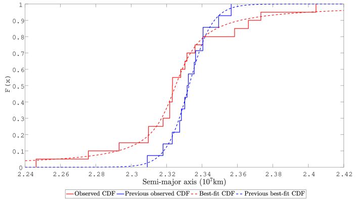
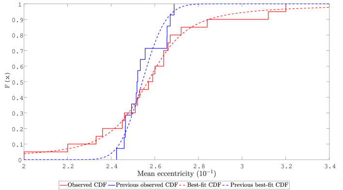
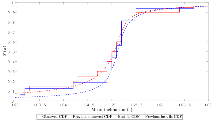
Figure 1. (a), (b) and (c) are the best-fitting CDF, the observed CDF of the current distributions and the observed CDF of the previous distributions, respectively, of the orbital characteristics of the moons in the Carme group

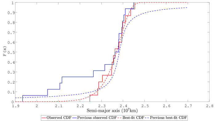
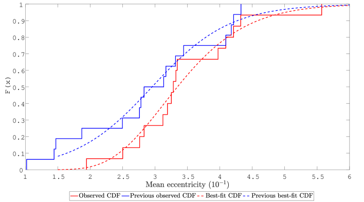
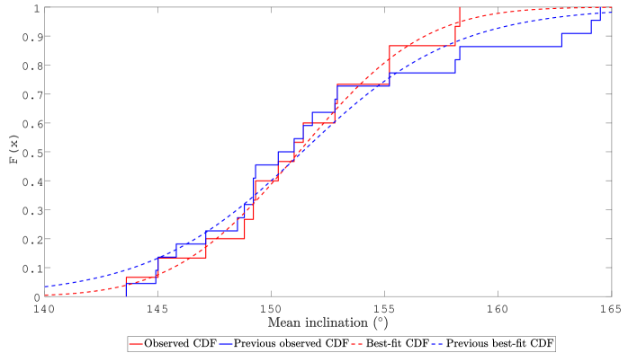
Figure 2. (a), (b) and (c) are the best-fitting CDF, the observed CDF of the current distributions and the observed CDF of the previous distributions, respectively, of the orbital characteristics of the moons in the Pasiphae group

4. Verification of the rationality of the theoretical results

In this section, the reasonability of the best-fitting distribution of the semi-major axis and the orbital period is demonstrated analytically based on Kepler’s third law of planetary motion.

4.1. Carme group

As seen from Table 2, for either the semi-major axis or the period, the distribution with the largest $p$-value, is a Stable distribution. However, as mentioned in Section 2, the probability density function (PDF) of the Stable distribution is given by the characteristic function. Three simple cases, namely, a Gaussian distribution, Cauchy distribution and Levy distribution, are not occurred, and it is difficult to calculate and draw the PDF. Therefore, we discuss the second largest $p$-value $t$ location-scale distribution. When the semi-major axis obeys the $t$ location-scale distribution, the $p$-value is 0.9000, and the parameters are 2.32508, 0.01141172, and 1.39731. When the period obeys a $t$ location-scale distribution, the $p$-value is 0.9792, and the parameters are 724.436, 6.75988, and 1.01233. The pdf of the $t$ location-scale distribution is given.

It can be seen from Table 2 that both the semi-major axis and the period obey a Stable distribution, and according to Kepler’s third law, there is a relationship $T=\sqrt{4\pi^{2}a^{3}/GM}$ ($G$ is the universal gravitational constant, and $M$ is the mass of Jupiter) between them. In theory, if the distribution type of the semi-major axis or the period is known, then the other one can be derived analytically. If the analysis results are consistent with the statistical inference results, or are at least very close, then the statistical inference results are valid. However, here, there is a problem, as described in Section 2, and the Stable distribution of the PDF can be given by the CF. The three special cases, namely, the Gaussian distribution, Cauchy distribution and Levy distribution are currently well studied, but in other Stable distributions, the PDFs are still poorly studied. Therefore, we have to discuss the distribution that is very close to its $p$-value, i.e. the $t$ location-scale distribution. When the semi-major axis obeys a $t$ location-scale distribution with a $p$-value of 0.9000, the corresponding parameters are 2.32508, 0.01141172, and 1.397731. When the period obeys a $t$ location-scale distribution of the $p$-value of 0.9792, the corresponding parameters are 724.436, 6.75988, and 1.01233.

Note that the PDF of the $t$ location-scale distribution can be defined as

(3) $$f= \frac{\Gamma(\frac{\nu+1}{2}))}{\sigma\sqrt{\nu\pi}\Gamma(\frac{\nu}{2}))}\left[\frac{\nu+(\frac{x-\mu}{\sigma})^{2}}{\nu}\right]^{-\frac{\nu+1}{2}},$$

where $\Gamma(\cdot)$ is the gamma function.

Therefore, the corresponding predicted PDFs can be written as

(4) $$f_{pre,\,a}(a;\mu,\sigma,\nu)=\frac{\Gamma(\frac{\nu+1}{2}))}{\sigma\sqrt{\nu\pi}\Gamma(\frac{\nu}{2}))}\left[\frac{\nu+(\frac{a-\mu}{\sigma})^{2}}{\nu}\right]^{-\frac{\nu+1}{2}}=\frac{23.884}{[1+0.716(70.836a-164.698)^{2}]^{1.199}},$$

and

(5) $$f_{pre,\,T}(T;\mu,\sigma,\nu)=\frac{\Gamma(\frac{\nu+1}{2}))}{\sigma\sqrt{\nu\pi}\Gamma(\frac{\nu}{2}))}\left[\frac{\nu+(\frac{T-\mu}{\sigma})^{2}}{\nu}\right]^{-\frac{\nu+1}{2}}=\frac{0.047}{[1+0.988(0.148a-107.181)^{2}]^{1.006}}.$$

Then, based on Kepler’s third law, the PDF of the semi-major axis can be derived as follows:

(6) $$f_{ana,a}(T;\mu,\sigma,\nu) =3\pi\sqrt{\frac{a}{GM}}f_{pre,T}(\sqrt{\frac{4\pi^{2}a^{3}}{GM}};724.436,6.75898,1.01233)$$

$$=\frac{14.475\sqrt{a}}{[1+0.988(30.245\sqrt{a^{3}}-107.181)^{2}]^{1.006}}.$$

From Figure 3 (a), we can find that $f_{ana,\,a}(T;\mu,\sigma,\nu)$ (the PDF is represented by the red curve) obtained by the analytical method is very similar to $f_{pre,\,a}(a;\mu,\sigma,\nu)$(the PDF is represented by the blue curve) obtained by statistical inference.

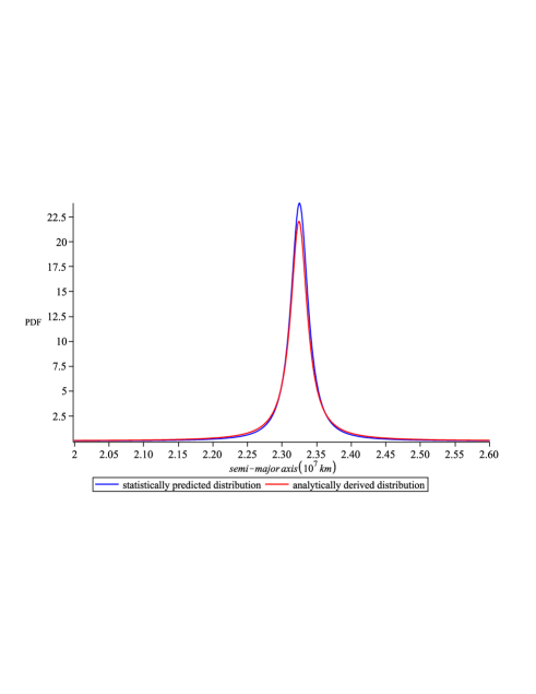
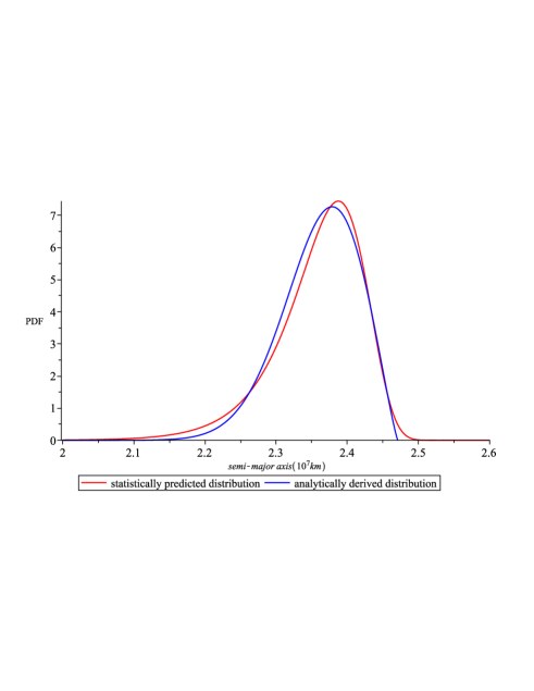
Figure 3. (a) and (b) are the PDFs of semi-major axis in the Carme group and the Pasiphae group, respectively

4.2. Pasiphae group

The corresponding predicted PDFs can be denoted by

(7) $$f_{pre,\,a}(a;\mu,\sigma)=\frac{e^{-\frac{a-\mu}{\sigma}}e^{-e^{\frac{a-\mu}{\sigma}}}}{\sigma}=20.247e^{20.247a-48.337}e^{-e^{20.247a-48.337}},$$

and

(8) $$f_{pre,\,T}(T;k,\mu,\sigma) =\frac{e^{-(1+((T-\mu)/\sigma)^{-1/k})}(1+k((T-\mu)/\sigma)^{-1-1/k})}{\sigma}$$

$$=0.371e^{-(13.458-0.017T)^{2.171}}(13.458-0.017T)^{1.171}.$$

Similarly, by using Kepler’s third law, the PDF of the semi-major axis can also be derived analytically as follows

(9) $$f_{ana,\,a}(T;\mu,\sigma) =3\pi\sqrt{\frac{a}{GM}}f_{pre,T}(\sqrt{\frac{4\pi^{2}a^{3}}{GM}};-0.460585,26.9631,729.292)$$

$$=11.284\sqrt{a}e^{-(13.458-3.465\sqrt{a^{3}})^{2.171}}(13.458-1.103\pi\sqrt{a^{3}})^{1.171}$$

From Figure 3 (b), we can also find that $f_{ana,\,a}(T;\mu,\sigma)$ (the PDF is represented by the blue curve) obtained by the analytical method is in good agreement with $f_{pre,\,T}(T;k,\mu,\sigma)$ (the PDF is represented by the red curve) obtained by statistical inference.

5. Conclusions

Based on reference [6], we use the K-S test to study the distributions of the orbital elements and orbital periods of the most recently discovered Jovial irregular moons in this paper. These orbital features mainly obey Stable, Extreme Value, Loglogistic, Generalized Extreme Value, Normal and Birnbaum-Saunders distributions.

Moreover, we also made some comparisons on the distributions of the semi-major axis, the mean eccentricity and the mean inclination. From the comparison results, the best-fitting distribution of the three features in this paper has the larger $p$-value. From the figures of best-fitting CDF and the CDF based on the observational data, the current best-fitting distribution and the previous one are well matched. There are two possible reasons for this result. First, the number of tested distribution functions is greater than that in [6]. Second, the classification of Jupiter’s moons has changed, and 12 newly discovered moons have been added. Furthermore, based on Kepler’s third law, the PDF obtained by the analytical method is very close to the PDF obtained by statistical inference, so it is reasonable to say that the best-fitting distribution of these orbital features is reasonable.

In addition, Table 5 shows that the orbital elements of some moons have the same Stable distribution. This interesting result may indicate that they have the same origin; they may have originated from the same parent asteroid. We will continue to study whether they are truly ‘siblings’.

Appendix

A. Classification of Irregular Moons

see Table 7

B. Orbital characteristics of Irregular Moons

see Table 8

C. Distribution Inference Results

See Tables 9-17

Table 7. Classification of irregular moons

Number	Name	Designation	Number	Name	Designation
Ananke group (Current)			Ananke group (Previous)
XXXIV	Euporie	S/2001 J10
LV		S/2003 J18
LII		S/2010 J2	LII		S/2010 J2
		S/2017 J7
LIV		S/2016 J1
		S/2017 J3
XXXIII	Euanthe	S/2001 J7	XXXIII	Euanthe	S/2001 J7
XXXV	Orthosie	S/2001 J9
XXIX	Thyone	S/2001 J2	XXIX	Thyone	S/2001 J2
XL	Mneme	S/2003 J21	XL	Mneme	S/2003 J21
XXII	Harpalyke	S/2000 J5	XXII	Harpalyke	S/2000 J5
XXX	Hermippe	S/2001 J3	XXX	Hermippe	S/2001 J3
XXVII	Praxidike	S/2000 J7	XXVII	Praxidike	S/2000 J7
XLII	Thelxinoe	S/2003 J22	XLII	Thelxinoe	S/2003 J22
LX		S/2003 J3	LX		S/2003 J3
XLV	Helike	S/2003 J6
XXIV	Iocaste	S/2000 J3	XXIV	Iocaste	S/2000 J3
XII	Ananke		XII	Ananke
		S/2017 J9
Carme group (Current)			Carme group (Previous)
		S/2003 J19
XLIII	Arche	S/2002 J1	XLIII	Arche	S/2002 J1
XXXVIII	Pasithee	S/2001 J6	XXXVIII	Pasithee	S/2001 J6
L	Herse	S/2003 J17	L	Herse	S/2003 J17
XXI	Chaldene	S/2000 J10	XXI	Chaldene	S/2000 J10
XXXVII	Kale	S/2001 J8	XXXVII	Kale	S/2001 J8
XXVI	Isonoe	S/2000 J6	XXVI	Isonoe	S/2000 J6
XXXI	Aitne	S/2001 J11	XXXI	Aitne	S/2001 J11
		S/2017 J5
		S/2017 J8
XXV	Erinome	S/2000 J4	XXV	Erinome	S/2000 J4
		S/2017 J2
LI		S/2010 J1	LI		S/2010 J1
XX	Taygets	S/2000 J9	XX	Taygets	S/2000 J9
XI	Carme		XI	Carme
XXIII	Kalyke	S/2000 J2	XXIII	Kalyke	S/2000 J2
XLVII	Eukelade	S/2003 J1	XLVII	Eukelade	S/2003 J1
LVII		S/2003 J5	LVII		S/2003 J5
XLIV	Kallichore	S/2003 J11	XLIV	Kallichore	S/2003 J11
		S/2011 J1
Pasiphae group (Current)			Pasiphae group (Previous)
		S/2017 J6
LVIII		S/2003 J15	LVIII		S/2003 J15
XXXII	Eurydome	S/2001 J4	XXXII	Eurydome	S/2001 J4
XXVIII	Autonoe	S/2001 J1	XXVIII	Autonoe	S/2001 J1
LVI		S/2011 J2	LVI		S/2011 J2
XXXVI	Sponde	S/2001 J5	XXXVI	Sponde	S/2001 J5
LIX		S/2017 J1	LIX		S/2017 J1
VIII	Pasiphae		VIII	Pasiphae
XIX	Megaclite	S/2000 J8	XIX	Megaclite	S/2000 J8
IX	Sinope		IX	Sinope
XXXIX	Hegemone	S/2003 J8	XXXIX	Hegemone	S/2003 J8
XLI	Aoede	S/2003 J7	XLI	Aoede	S/2003 J7
XVII	Callirrhoe	S/1999 J1	XVII	Callirrhoe	S/1999 J1
XLVIII	Cyllene	S/2003 J13	XLVIII	Cyllene	S/2003 J13
XLIX	Kore	S/2003 J14	XLIX	Kore	S/2003 J14
			XXXIV	Euporie	S/2001 J10
			LV		S/2003 J18
			LIV		S/2016 J1
			XXXV	Orthosie	S/2001 J9
			XLV	Helike	S/2003 J6

Table 8. Orbital characteristics of irregular moons in Ananke, Carme and Pasiphae groups¹

Ananke group
Number	Name	Designation	Mean semi-major axis (km)	Mean inclination (deg)	Mean eccentricity	Peri (deg)	Node (deg)	Period (days)
XXXIV	Euporie	S/2001 J10	19302000	145.8	0.144	74.6	64.9	550.7
LV		S/2003 J18	20274000	146.4	0.105	98.15	215.5	588
LII		S/2010 J2	20307150	150.4	0.307	0	0	588.1
		S/2017 J7	20627000	143.4	0.215	323.5	321.5	602.6
LIV		S/2016 J1	20650845	139.8	0.141	328.2	293.8	602.7
		S/2017 J3	20694000	147.9	0.148	171.6	82.5	606.3
XXXIII	Euanthe	S/2001 J7	20799000	148.9	0.232	316	271	620.6
XXXV	Orthosie	S/2001 J9	20721000	145.9	0.281	230.5	223.6	622.6
XXIX	Thyone	S/2001 J2	20940000	148.5	0.229	89.1	243	627.3
XL	Mneme	S/2003 J21	21069000	148.6	0.227	41.7	18.1	620
XXII	Harpalyke	S/2000 J5	21105000	148.6	0.226	129.9	40	623.3
XXX	Hermippe	S/2001 J3	21131000	150.7	0.21	298.7	347.2	633.9
XXVII	Praxidike	S/2000 J7	21147000	149	0.23	209.7	285.2	625.3
XLII	Thelxinoe	S/2003 J22	21162000	151.4	0.221	179.8	206.2	628.1
LX		S/2003 J3	21199710	148	0.253	109	292	627.8
XLV	Helike	S/2003 J6	21263000	154.8	0.156	314.7	100.3	634.8
XXIV	Iocaste	S/2000 J3	21269000	149.4	0.216	80	271.3	631.5
XII	Ananke		21276000	148.9	0.244	100.6	7.6	610.5
		S/2017 J9	21487000	152.7	0.229	317.7	306.4	639.2
Carme group
Number	Name	Designation	Mean semi-major axis (km)	Mean inclination (deg)	Mean eccentricity	Peri (deg)	Node (deg)	Period (days)
		S/2003 J19	22757000	166.7	0.257	284.1	105.7	697.6
XLIII	Arche	S/2002 J1	22931000	165	0.259	161.1	350.7	723.9
XXXVIII	Pasithee	S/2001 J6	23096000	165.1	0.267	253.3	338.7	719.5
L	Herse	S/2003 J17	23097000	164.2	0.2	355.7	329	715.4
XXI	Chaldene	S/2000 J10	23179000	165.2	0.251	282.5	148.7	723.8
XXXVII	Kale	S/2001 J8	23217000	165	0.26	44.4	56.4	729.5
XXVI	Isonoe	S/2000 J6	23217000	165.2	0.246	145.6	149.8	725.5
XXXI	Aitne	S/2001 J11	23231000	165.1	0.264	122.2	24.5	730.2
		S/2017 J5	23232000	164.3	0.284	11.9	118.2	719.5
		S/2017 J8	23232700	164.7	0.312	45.1	160.3	719.6
XXV	Erinome	S/2000 J4	23279000	164.9	0.266	356	321.7	728.3
		S/2017 J2	23303000	166.4	0.236	231.9	74.7	723.1
LI		S/2010 J1	23314335	163.2	0.32	0	0	723.2
XX	Taygets	S/2000 J9	23360000	165.2	0.252	241.1	313.3	732.2
XI	Carme		23404000	164.9	0.253	28.2	113.7	702.3
XXIII	Kalyke	S/2000 J2	23583000	165.2	0.245	216.6	38.7	743
XLVII	Eukelade	S/2003 J1	23661000	165.5	0.272	325.6	206.3	746.4
LVII		S/2003 J5	23731770	163.1	0.22	160	256.3	759.7
XLIV	Kallichore	S/2003 J11	24043000	165.5	0.264	18.5	41.5	764.7
		S/2011 J1	22462000	163.3	0.233	127.2	323.9	580.7
Pasiphae group
Number	Name	Designation	Mean semi-major axis (km)	Mean inclination (deg)	Mean eccentricity	Peri (deg)	Node (deg)	Period (days)
		S/2017 J6	22455000	155.2	0.557	77.3	26.3	683
LVIII		S/2003 J15	22819950	143.6	0.194	52.08	286.5	701.3
XXXII	Eurydome	S/2001 J4	22865000	150.3	0.276	241.6	307.4	717.3
XXVIII	Autonoe	S/2001 J1	23039000	152.9	0.334	60.2	275.6	762.7
LVI		S/2011 J2	23463885	148.8	0.332	341.9	105.2	730.5
XXXVI	Sponde	S/2001 J5	23487000	151	0.312	79.1	129.1	748.3
LIX		S/2017 J1	23547105	149.2	0.397	79.73	326.8	734.2
VIII	Pasiphae		23624000	151.4	0.409	170.5	313	708
XIX	Megaclite	S/2000 J8	23806000	152.8	0.421	302.3	304.6	752.8
IX	Sinope		23939000	158.1	0.25	346.4	303.1	724.5
XXXIX	Hegemone	S/2003 J8	23947000	155.2	0.328	235.4	327.6	739.6
XLI	Aoede	S/2003 J7	23981000	158.3	0.432	74.5	187.1	761.5
XVII	Callirrhoe	S/1999 J1	24102000	147.1	0.283	49.3	281.1	758.8
XLVIII	Cyllene	S/2003 J13	24349000	149.3	0.319	214	266.4	737.8
XLIX	Kore	S/2003 J14	24543000	145	0.325	152.4	324.7	779.2

Table 9. Ananke group

		Beta	Birnbaum- Saunders	Exponential	Extreme Value	Gamma	Generalized Extreme Value	Generalized Pareto	Half Normal	Logistic	Loglogistic
	h	0	0	1	0	0	0	1	1	0	0
	p	0.4579	0.4559	0	0.6775	0.4573	0.7485	0	0	0.6669	0.6644
Semi-major axis(km)	parameters	a=1397.16 b=5299.25	$\beta$=2.08584e+07 $\gamma$=0.0240486	$\mu$=2.08644e+07	$\mu$=2.10699e+07 $\sigma$=326466	a=1753.38 b=11899.5	k=-0.744702 $\sigma$=519095 $\mu$=2.08073e+07	k=-1.71428 $\sigma$=3.68346e+07 $\theta$=0	$\mu$=0 $\sigma$=2.08702e+07	$\mu$=2.09326e+07 $\sigma$=251319	$\alpha$=16.8567 $\beta$=0.0121476
	confidence interval	a$\epsilon$[769.666, 2536.25] b$\epsilon$[2875.3, 9766.65]	$\beta$$\epsilon$[[2.06328e+07, 2.10839e+07] $\gamma$$\epsilon$[0.0164024, 0.0316948]	$\mu$$\epsilon$[1.39351e+07, 3.46547e+07]	$\mu$$\epsilon$[2.09165e+07, 2.12234e+07] $\sigma$$\epsilon$[225567, 472498]	a$\epsilon$[928.403, 3311.44] b$\epsilon$[6300.14, 22475.5]	k$\epsilon$[-1.06557, -0.423836] $\sigma$$\epsilon$[342491, 786765] $\mu$$\epsilon$[2.05563e+07, 2.10584e+07]	k$\epsilon$[-1.71428, -1.71428] $\sigma$$\epsilon$[3.68346e+07, 3.68346e+07] $\theta$=0	$\mu$=0 $\sigma$$\epsilon$[1.58716e+07, 3.04824e+07]	$\mu$$\epsilon$[2.07385e+07, 2.11266e+07] $\sigma$$\epsilon$[172051, 367108]	$\alpha$$\epsilon$[16.8473 ,16.8661] $\beta$$\epsilon$[0.00831, 0.01776]
		Lognormal	Nakagami	Normal	Poisson	Rayleigh	Rician	Stable	T location- Scale	Weibull
	h	0	0	1	1	1	0	0	0	0
	p	0.4836	0.4584	0.4874	0	0	0.4416	0.9118	0.7030	0.6530
Semi-major axis(km)	parameters	$\mu$=16.8533 $\sigma$=0.0247039	$\mu$=444.399 $\omega$=4.35565e+14	$\mu$=2.086e+07 $\sigma$=505144	$\lambda$=2.08644e+07	B=1.47575e+07	s=2.0859e+07 $\sigma$=482376	$\alpha$=1.32899 $\beta$=-1 $\gamma$=211134 $\delta$=2.107e+07	$\mu$= 2.09727e+07 $\sigma$=323763 $\nu$=3.25004	A=2.1067e+07 B=63.7906
	confidence interval	$\mu$$\epsilon$[16.8414, 16.8652] $\sigma$$\epsilon$[0.0186666, 0.0365328]	$\mu$$\epsilon$[235.346, 839.149] $\omega$$\epsilon$[4.26373e+14, 4.44955e+14]	$\mu$$\epsilon$[2.06209e+07, 2.11079e+07] $\sigma$$\epsilon$[381693, 747019]	$\lambda$$\epsilon$[2.08624e+07, 2.08665e+07]	B$\epsilon$[1.20605e+07, 1.90191e+07]	s$\epsilon$[2.06421e+07, 2.1076e+07] $\sigma$$\epsilon$[354124, 657076]	$\alpha$$\epsilon$[0, 2] $\beta$$\epsilon$[-1, 1] $\gamma$$\epsilon$[0, Inf] $\delta$$\epsilon$[-Inf, Inf]	$\mu$$\epsilon$[2.07742e+07, 2.11712e+07] $\sigma$$\epsilon$[188792, 555228] $\nu$$\epsilon$[0.749091, 14.1008]	A$\epsilon$[2.09125e+07, 2.12227e+07] B$\epsilon$[44.0088, 92.4642]
		Beta	Birnbaum- Saunders	Exponential	Extreme Value	Gamma	Generalized Extreme Value	Generalized Pareto	Half Normal	Logistic	Loglogistic
	h	0	0	1	0	0	0	1	1	0	0
	p	0.5068	0.4922	0	0.6041	0.5031	0.6695	0	0	0.7882	0.7767
Mean inclination (deg)	parameter	a=1802.04 b=10343.3	$\beta$=148.338 $\gamma$=0.0218171	$\mu$=148.374	$\mu$=149.899 $\sigma$=2.92228	a= 2112.35 b=0.0702412	k=-0.390871 $\sigma$=3.44763 $\mu$=147.409	k=-1.77721 $\sigma$=275.112 $\theta$=0	$\mu$=0 $\sigma$=148.408	$\mu$=148.551 $\sigma$=1.69405	$\alpha$=5.00086 $\beta$=0.0114546
	confidence interval	a$\epsilon$[1045.98, 3104.61] b$\epsilon$[5974.94, 17905.3]	$\beta$$\epsilon$ [149.038, 153.273] $\gamma$$\epsilon$ [0.0177789, 0.0375931]	$\mu$$\epsilon$[99.0974, 246.441]	$\mu$$\epsilon$[148.508, 151.29] $\sigma$$\epsilon$[2.10881, 4.04954]	a$\epsilon$[1118.46, 3989.42] b$\epsilon$[0.037189, 0.132669]	k$\epsilon$[-0.625452, -0.156291] $\sigma$$\epsilon$[2.46918, 4.81381] $\mu$$\epsilon$[145.733, 149.085]	k$\epsilon$[-Inf, -1.77721] $\sigma$$\epsilon$[-Inf, 275.112] $\theta$=0	$\mu$=0 $\sigma$$\epsilon$[112.863, 216.761]	$\mu$$\epsilon$[147.257, 149.844] $\sigma$$\epsilon$[1.15043, 2.49456]	$\alpha$$\epsilon$[4.99212, 5.00959] $\beta$$\epsilon$[0.00777713, 0.0168709]
		Lognormal	Nakagami	Normal	Poisson	Rayleigh	Rician	Stable	T location- Scale	Weibull
	h	0	0	0	1	1	0	0	0	0
	p	0.4826	0.5138	0.5138	0.0402	0	0.5248	0.9109	0.9039	0.6304
Mean inclination (deg)	parameter	$\mu$=4.9995 $\sigma$=0.0224131	$\mu$=530.921 $\omega$=22025.1	$\mu$=148.374 $\sigma$=3.30031	$\lambda$=148.374	B=104.941	s=148.339 $\sigma$=3.21266	$\alpha$=1.42053 $\beta$=-0.205584 $\gamma$=1.62162 $\delta$ =148.744	$\mu$=148.668 $\sigma$=1.93018 $\nu$=2.34369	A=149.869 B= 51.3526
	confidence interval	$\mu$$\epsilon$[4.98869, 5.0103] $\sigma$$\epsilon$[0.0169356, 0.033145]	$\mu$$\epsilon$[281.157, 1002.56] $\omega$$\epsilon$[21599.4, 22459.1]	$\mu$$\epsilon$[146.783, 149.964] $\sigma$$\epsilon$[2.49376, 4.88058]	$\lambda$$\epsilon$[142.897, 153.851]	B$\epsilon$[85.7623, 135.245]	s$\epsilon$[146.894, 149.784] $\sigma$$\epsilon$[2.33748, 4.41553]	$\alpha$$\epsilon$[0.746773, 2] $\beta$$\epsilon$[-1, 0.999048] $\gamma$$\epsilon$[0.8027, 2.44053] $\delta$$\epsilon$147.487, 150.002]	$\mu$$\epsilon$[147.592, 149.745] $\sigma$$\epsilon$[0.792217, 4.70273] $\nu$$\epsilon$[0.367785, 14.935]	A$\epsilon$[148.488, 151.264] B$\epsilon$[36.9937, 71.2849]

Table 10. Ananke group (Cont’d)

		Beta	Birnbaum- Saunders	Exponential	Extreme Value	Gamma	Generalized Extreme Value	Generalized Pareto	Half Normal	Logistic	Loglogistic
	h	0	0	1	0	0	0	1	1	0	0
	p	0.1478	0.0828	0.0009	0.4945	0.1254	0.3551	0.0145	0.0010	0.4336	0.2711
Mean eccentricity	parameter	a=12.9547 b=48.4209	$\beta$=0.204059 $\gamma$=0.265447	$\mu$=0.211263	$\mu$=0.235049 $\sigma$=0.0444536	a=15.8753 b=0.0133076	k=-0.39185 $\sigma$ = 0.0523617 $\mu$=0.196366	k=-1.21873 $\sigma$=0.37415 $\theta$=0	$\mu$= 0 $\sigma$=0.216997	$\mu$=0.21506 $\sigma$=0.0279307	$\alpha$=-1.55125 $\beta$=0.14478
	confidence interval	a$\epsilon$[6.45226, 26.0102] b$\epsilon$[22.0396, 106.38]	$\beta$$\epsilon$[0.179918, 0.2282] $\gamma$$\epsilon$[0.181049, 0.349846]	$\mu$$\epsilon$[0.141101, 0.350897]	$\mu$$\epsilon$[0.213908, 0.256189] $\sigma$$\epsilon$[0.0318622, 0.0620209]	a$\epsilon$[8.46076, 29.7877] b$\epsilon$[0.00702145, 0.0252217]	k$\epsilon$[-0.661953, -0.121748] $\sigma$$\epsilon$[0.036903, 0.0742961] $\mu$$\epsilon$[0.170663, 0.22207]	k$\epsilon$[-Inf, -1.21873] $\sigma$$\epsilon$[-Inf, 0.37415] $\theta$=0	$\mu$ = 0 $\sigma$$\epsilon$[0.165024, 0.31694]	$\mu$$\epsilon$[0.193301, 0.236819] $\sigma$$\epsilon$[0.019043, 0.0409666]	$\alpha$$\epsilon$[-1.66398, 1.43853] $\beta$$\epsilon$[0.0983852, 0.213054]
		Lognormal	Nakagami	Normal	Poisson	Rayleigh	Rician	Stable	T location- Scale	Weibull
	h	0	0	0	1	1	0	0	0	0
	p	0.0925	0.1682	0.2423	0	0.0160	0.2387	0.3123	0.2434	0.3578
Mean eccentricity	parameter	$\mu$=-1.58648 $\sigma$=0.270232	$\mu$=4.42555 $\omega$=0.0470879	$\mu$=0.211263 $\sigma$=0.0509137	$\lambda$ =0.211263	B=0.15344	s=0.204966 $\sigma$=0.0503827	$\alpha$=1.89626 $\beta$=-1 $\gamma$=0.0340103 $\delta$ =0.21524	$\mu$=0.211262 $\sigma$=0.0495574 $\nu$=3.98736e+06	A=0.23032 B=5.0073
	confidence interval	$\mu$$\epsilon$[-1.71672,-1.45623] $\sigma$$\epsilon$[0.20419,0.399625]	$\mu$$\epsilon$[2.39638, 8.17293] $\omega$$\epsilon$[0.0380262, 0.058309]	$\mu$$\epsilon$[0.186724, 0.235803] $\sigma$$\epsilon$[0.038471, 0.0752924]	$\lambda$$\epsilon$[0.0577346, 0.540098]	B$\epsilon$[0.125399, 0.197751]	s$\epsilon$[0.181539, 0.228393] $\sigma$$\epsilon$[0.0362405, 0.0700438]	$\alpha$$\epsilon$[0, 2] $\beta$$\epsilon$[-1, 1] $\gamma$ $\epsilon$[0, Inf] $\delta$$\epsilon$[-Inf, Inf]	$\mu$$\epsilon$[0.188982, 0.233543] $\sigma$$\epsilon$[0.0360595, 0.0681077] $\nu$$\epsilon$[2.13985e+06, 7.42999e+06]	A$\epsilon$[0.209584, 0.253108] B$\epsilon$[3.51102, 7.14124]
		Beta	Birnbaum- Saunders	Exponential	Extreme Value	Gamma	Generalized Extreme Value	Generalized Pareto	Half Normal	Logistic	Loglogistic
	h	0	0	0	0	0	0	0	0	0	0
	p	0.4979	0.5451	0.1202	0.5029	0.5062	0.4524	0.3770	0.3221	0.4721	0.6543
Argument of periapsis	parameter	a=2.59874 b=11.1496	$\beta$=157.229 $\gamma$=0.638662	$\mu$=189.636	$\mu$=240.599 $\sigma$=91.6541	a=3.08052 b=61.5598	k=-1.06385 $\sigma$=155.122 $\mu$=182.388	k=-1.21079 $\sigma$=397.382 $\theta$=0	$\mu$=0 $\sigma$=214.793	$\mu$=185.934 $\sigma$=62.8644	$\alpha$=5.10234 $\beta$=0.374292
	confidence interval	a$\epsilon$ [0.916259, 7.3707] b$\epsilon$[3.41356, 36.4178]	$\beta$$\epsilon$ [113.211, 201.247] $\gamma$$\epsilon$ [0.430034, 0.84729]	$\mu$$\epsilon$[125.409, 319.973]	$\mu$$\epsilon$[195.735, 285.463] $\sigma$$\epsilon$ [63.658, 131.962]	a$\epsilon$[1.65515, 5.73336] b$\epsilon$[31.3541, 120.865]	k$\epsilon$[-Inf, Inf] $\sigma$$\epsilon$[0, Inf] $\mu$$\epsilon$[-Inf, Inf]	k$\epsilon$[-1.21079, Inf] $\sigma$$\epsilon$[-Inf, Inf] $\theta$=0	$\mu$=0 $\sigma$$\epsilon$[162.3, 317.641]	$\mu$$\epsilon$[133.271, 238.596] $\sigma$$\epsilon$[43.5501, 90.7446]	$\alpha$$\epsilon$[4.79185, 5.41282] $\beta$$\epsilon$[0.258487, 0.541979]
		Lognormal	Nakagami	Normal	Poisson	Rayleigh	Rician	Stable	T location- Scale	Weibull
	h	0	0	0	1	0	0	0	0	0
	p	0.6118	0.4918	0.4992	0.0009	0.4852	0.4779	0.4538	0.4537	0.4856
Argument of periapsis	parameter	$\mu$=5.0741 $\sigma$=0.635986	$\mu$=0.978907 $\omega$=46135.8	$\mu$=189.636 $\sigma$=103.79	$\lambda$= 189.636	B=151.881	s=110.961 $\sigma$=130.046	$\alpha$=2 $\beta$=-0.999998 $\gamma$=71.3235 $\delta$=189.637	$\mu$=189.631 $\sigma$=100.865 $\nu$=6.77805e+06	A=214.751 B=1.9981
	confidence interval	$\mu$$\epsilon$[4.75783, 5.39037] $\sigma$$\epsilon$[0.477236, 0.953435]	$\mu$$\epsilon$[0.5513, 1.73818] $\omega$$\epsilon$[28924, 73590]	$\mu$$\epsilon$[138.022, 241.25] $\sigma$$\epsilon$[77.8831, 155.597]	$\lambda$$\epsilon$[183.274, 195.998]	B$\epsilon$[123.511, 197.288]	s$\epsilon$[0, 315.078] $\sigma$$\epsilon$[65.8599, 256.788]	$\alpha$$\epsilon$[0, 2] $\beta$$\epsilon$[-1, 1] $\gamma$$\epsilon$[0, Inf] $\delta$$\epsilon$[-Inf, Inf]	$\mu$$\epsilon$[142.009, 237.253] $\sigma$$\epsilon$[71.3916, 142.507] $\nu$$\epsilon$[4.36477e+06, 1.05256e+07]	A$\epsilon$[168.289, 274.04] B[1.37039, 2.91335]

Table 11. Ananke group (Cont’d)

		Beta	Birnbaum- Saunders	Exponential	Extreme Value	Gamma	Generalized Extreme Value	Generalized Pareto	Half Normal	Logistic	Loglogistic
	h	0	1	1	0	0	0	0	0	0	0
	p	0.1048	0.0078	0.0481	0.5642	0.0805	0.7088	0.3828	0.0621	0.6178	0.1824
Longitude of the ascending node	parameter	a=1.42533 b=5.95015	$\beta$=102.405 $\gamma$=1.27373	$\mu$=199.45	$\mu$=251.496 $\sigma$=85.2376	a=1.5648 b=127.46	k=-0.784386 $\sigma$=127.426 $\mu$=188.251	k=-1.16562 $\sigma$=404.703 $\theta$=0	$\mu$=0 $\sigma$=228.379	$\mu$=210.223 $\sigma$=67.3575	$\alpha$=5.14311 $\beta$=0.562338
	confidence interval	a$\epsilon$[0.686733, 2.95831] b$\epsilon$[1.49282, 23.7164]	$\beta$$\epsilon$ [52.7286, 152.082] $\gamma$$\epsilon$[0.854416, 1.69304]	$\mu$$\epsilon$[131.899, 336.532]	$\mu$$\epsilon$[210.108, 292.884] $\sigma$$\epsilon$[58.0581, 125.141]	a$\epsilon$[0.861677, 2.84167] b$\epsilon$[63.1887, 257.105]	k$\epsilon$[-1.1982, -0.370575] $\sigma$$\epsilon$[79.4528, 204.364] $\mu$$\epsilon$[124.222, 252.28]	k$\epsilon$[-1.16562, -1.16562] $\sigma$$\epsilon$[404.703, 404.703] $\theta$=0	$\mu$= 0 $\sigma$$\epsilon$[172.566, 337.732]	$\mu$$\epsilon$[154.35, 266.095] $\sigma$$\epsilon$[46.2235, 98.1541]	$\alpha$$\epsilon$[4.69465, 5.59157] $\beta$$\epsilon$[0.377227, 0.838284]
		Lognormal	Nakagami	Normal	Poisson	Rayleigh	Rician	Stable	T location- Scale	Weibull
	h	0	0	0	1	0	0	0	0	0
	p	0.0576	0.1090	0.4757	0.0001	0.2820	0.4212	0.4712	0.4709	0.1297
Longitude of the ascending node	parameter	$\mu$=4.94319 $\sigma$=1.10303	$\mu$=0.628956 $\omega$= 52157	$\mu$=199.45 $\sigma$=114.476	$\lambda$=199.45	B=161.488	s=149.14 $\sigma$=122.3	$\alpha$=2 $\beta$=-1 $\gamma$=78.667 $\delta$=199.449	$\mu$=199.435 $\sigma$=111.246 $\nu$=6.46968e+06	A=218.256 B=1.57172
	confidence interval	$\mu$$\epsilon$[4.39467, 5.49172] $\sigma$$\epsilon$[0.827703, 1.65361]	$\mu$$\epsilon$[0.362485, 1.09131] $\omega$$\epsilon$[29129.5, 93388.3]	$\mu$$\epsilon$[142.523, 256.377] $\sigma$$\epsilon$[85.9012, 171.616]	$\lambda$$\epsilon$[192.926, 205.974]	B$\epsilon$[131.324, 209.767]	s$\epsilon$[52.4982, 245.782] $\sigma$$\epsilon$[77.6676, 192.581]	$\alpha$$\epsilon$[0, 2] $\beta$$\epsilon$[-1, 1] $\gamma$ $\epsilon$[0, Inf] $\delta$$\epsilon$[-Inf, Inf]	$\mu$$\epsilon$[148.886, 249.985] $\sigma$$\epsilon$[81.3445,152.139] $\nu$$\epsilon$[3.91848e+06,1.06819e+07]	A$\epsilon$[160.929, 296.004] B$\epsilon$[1.03829, 2.37921]
		Beta	Birnbaum- Saunders	Exponential	Extreme Value	Gamma	Generalized Extreme Value	Generalized Pareto	Half Normal	Logistic	Loglogistic
	h	0	0	1	0	0	0	1	1	0	0
	p	0.2465	0.2242	0	0.6216	0.2296	0.9351	0	0	0.5353	0.5154
Period (days)	parameter	a=335.873 b=210.358	$\beta$=614.532 $\gamma$=0.0351084	$\mu$=614.911	$\mu$=623.735 $\sigma$=13.7502	a=827.283 b=0.743289	k=-0.870222 $\sigma$=22.3828 $\mu$=613.723	k=-2.42026 $\sigma$=1547.03 $\theta$=0	$\mu$=0 $\sigma$=615.269	$\mu$=618.02 $\sigma$=10.9316	$\alpha$=6.42625 $\beta$=0.0180128
	confidence interval	a$\epsilon$[176.163, 640.38] b$\epsilon$[105.692, 418.675]	$\beta$$\epsilon$[604.832,624.232] $\gamma$$\epsilon$[0.0239457, 0.046271]	$\mu$$\epsilon$[410.693, 1021.34]	$\mu$$\epsilon$[617.279, 630.19] $\sigma$$\epsilon$[9.43218, 20.045]	a$\epsilon$[438.07, 1562.3] b$\epsilon$[0.393517, 1.40395]	k$\epsilon$[-1.28411, -0.456332] $\sigma$$\epsilon$[13.914, 36.0062] $\mu$$\epsilon$[602.793, 624.652]	k$\epsilon$[-2.42026, -2.42026] $\sigma$$\epsilon$[1547.03, 1547.03] $\theta$=0	$\mu$=0 $\sigma$$\epsilon$[467.906, 898.644]	$\mu$$\epsilon$[609.549, 626.491] $\sigma$$\epsilon$[7.47098, 15.9953]	$\alpha$$\epsilon$[6.41233, 6.44017] $\beta$$\epsilon$[0.0122975, 0.0263843]
		Lognormal	Nakagami	Normal	Poisson	Rayleigh	Rician	Stable	T location- Scale	Weibull
	h	0	0	0	0	1	0	0	0	0
	p	0.2356	0.2346	0.2515	0.2590	0	0.2404	0.9878	0.8519	0.5766
Period (days)	parameter	$\mu$=6.42087 $\sigma$=0.0360603	$\mu$=210.823 $\omega$=378556	$\mu$=614.911 $\sigma$=21.565	$\lambda$=614.911	B=435.061	s=614.552 $\sigma$=20.9959	$\alpha$=1.20629 $\beta$=-1 $\gamma$=8.28652 $\delta$=624.981	$\mu$=620.502 $\sigma$=13.4808 $\nu$=2.87835	A=623.556 B=44.4899
	confidence interval	$\mu$$\epsilon$[6.40349, 6.43825] $\sigma$$\epsilon$[0.0272476, 0.0533268]	$\mu$$\epsilon$[111.68,397.981] $\omega$$\epsilon$[367012,390462]	$\mu$$\epsilon$[604.517, 625.305] $\sigma$$\epsilon$[16.2948, 31.8909]	$\lambda$$\epsilon$[603.76, 626.061]	B$\epsilon$[355.552, 560.697]	s$\epsilon$[605.106, 623.998] $\sigma$$\epsilon$[15.2746, 28.86]	$\alpha$$\epsilon$[0, 2] $\beta$$\epsilon$[-1, 1] $\gamma$$\epsilon$[0, Inf] $\delta$$\epsilon$[-Inf, Inf]	$\mu$$\epsilon$[610.751, 630.252] $\sigma$$\epsilon$[6.67616, 27.221] $\nu$$\epsilon$[0.49418, 16.765]	A$\epsilon$[617.017, 630.164] B$\epsilon$[30.4616, 64.9787]

Table 12. Carme group

		Beta	Birnbaum- Saunders	Exponential	Extreme Value	Gamma	Generalized Extreme Value	Generalized Pareto	Half Normal	Logistic	Loglogistic
	h	0	0	1	0	0	0	1	1	0	0
	p	0.6707	0.6626	0	0.3564	0.6678	0.6141	0	0	0.8347	0.8297
Semi-major axis(km)	parameter	a=3773.99 b=12446.7	$\beta$=2.32642e+07 $\gamma$=0.0142652	$\mu$=2.32665e+07	$\mu$=2.34332e+07 $\sigma$=340905	a=4917.14 b=4731.72	k=-0.275087 $\sigma$=339070 $\mu$=2.31489e+07	k=-1.80798 $\sigma$=4.34692e+07 $\theta$=4.34692e+07	$\mu$=0 $\sigma$=2.32689e+07	$\mu$=2.3265e+07 $\sigma$=174602	$\alpha$=16.9624 $\beta$=0.00750411
	confidence interval	a$\epsilon$[2258.13, 6307.43] b$\epsilon$[7444.41, 20810.2]	$\beta$$\epsilon$[2.31187e+07, 2.34096e+07] $\gamma$$\epsilon$[0.00984445, 0.018686]	$\mu$$\epsilon$[1.56831e+07, 3.80903e+07]	$\mu$$\epsilon$[2.32745e+07, 2.35919e+07] $\sigma$$\epsilon$[250817, 463349]	a$\epsilon$[2645.74, 9138.54] b$\epsilon$[2545.9, 8794.23]	k$\epsilon$ [-0.496047, -0.0541257] $\sigma$$\epsilon$[247035, 465394] $\mu$$\epsilon$[2.29877e+07, 2.33101e+07]	k$\epsilon$[-1.80798, Inf] $\sigma$$\epsilon$[-Inf, Inf] $\theta$=0	$\mu$=0 $\sigma$$\epsilon$[1.78021e+07, 3.36019e+07]	$\mu$$\epsilon$[2.31357e+07, 2.33943e+07] $\sigma$$\epsilon$[119319, 255498]	$\alpha$$\epsilon$[16.9569, 16.968] $\beta$$\epsilon$[0.00512804, 0.0109811]
		Lognormal	Nakagami	Normal	Poisson	Rayleigh	Rician	Stable	T location- Scale	Weibull
	h	0	0	0	1	1	0	0	0	0
	p	0.6282	0.6726	0.6428	0	0	0.6780	0.9534	0.9000	0.3721
Semi-major axis(km)	parameter	$\mu$=16.9624 $\sigma$=0.0146353	$\mu$=1230.01 $\omega$=5.41442e+14	$\mu$=2.32665e+07 $\sigma$=340277	$\lambda$=2.32665e+07	B =1.64536e+07	s=2.32642e+07 $\sigma$=331568	$\alpha$=0.987755 $\beta$=0.0533906 $\gamma$=112441 $\delta$=2.32477e+07	$\mu$=2.32508e+07 $\sigma$=141172 $\nu$=1.39731	A=2.34307e+07 B=68.9778
	confidence interval	$\mu$$\epsilon$[16.9556, 16.9693] $\sigma$$\epsilon$[0.01113, 0.0213759]	$\mu$$\epsilon$[661.944, 2285.56] $\omega$$\epsilon$ [5.34718e+14, 5.4825e+14]	$\mu$$\epsilon$[2.31073e+07, 2.34258e+07] $\sigma$$\epsilon$[258777, 496999]	$\lambda$$\epsilon$[2.32644e+07, 2.32687e+07]	B$\epsilon$[1.35086e+07, 2.10524e+07]	s$\epsilon$[2.31189e+07, 2.34095e+07] $\sigma$$\epsilon$[243242, 451966]	$\alpha$$\epsilon$[0, 2] $\beta$$\epsilon$[-1,1] $\gamma$$\epsilon$[0, Inf] $\delta$$\epsilon$[-Inf, Inf]	$\mu$$\epsilon$[2.31715e+07, 2.33301e+07] $\sigma$$\epsilon$[48245.8, 413086] $\nu$$\epsilon$[0.35453, 5.50721]	A$\epsilon$[2.32731e+07, 2.35893e+07] B$\epsilon$[50.6995, 93.8459]
		Beta	Birnbaum- Saunders	Exponential	Extreme Value	Gamma	Generalized Extreme Value	Generalized Pareto	Half Normal	Logistic	Loglogistic
	h	0	0	1	0	0	0	1	1	0	0
	p	0.3122	0.3095	0	0.2440	0.3115	0.4135	0	0	0.4868	0.4839
Mean inclination (deg)	parameter	a=27924 b=141430	$\beta$=164.883 $\gamma$=0.00547125	$\mu$=164.885	$\mu$=165.323 $\sigma$=0.845915	a=33428 b=0.00493254	k=-0.356257 $\sigma$=0.945989 $\mu$=164.599	k=-1.83956 $\sigma$=306.654 $\theta$=0	$\mu$=0 $\sigma$=164.887	$\mu$= 164.941 $\sigma$=0.486932	$\alpha$=5.10558 $\beta$=0.00295561
	confidence interval	a$\epsilon$[15057.1, 51786.1] b$\epsilon$[76208.3, 262472]	$\beta$$\epsilon$[164.487, 165.278] $\gamma$$\epsilon$[0.00377572, 0.00716679]	$\mu$$\epsilon$[111.143, 269.938]	$\mu$$\epsilon$[164.93, 165.715] $\sigma$$\epsilon$[0.615862, 1.1619]	a$\epsilon$[17986.2, 62127.3] b$\epsilon$[0.00265397, 0.00916737]	k$\epsilon$ [-0.613099, -0.0994139] $\sigma$$\epsilon$[0.678189, 1.31954] $\mu$$\epsilon$[164.146, 165.051]	k$\epsilon$[-1.83956, -1.83956] $\sigma$$\epsilon$[306.654, 306.654] $\theta$=0	$\mu$=0 $\sigma$$\epsilon$[126.149, 238.109]	$\mu$$\epsilon$[164.578, 165.303] $\sigma$$\epsilon$[0.332449, 0.7132]	$\alpha$$\epsilon$[5.10338, 5.10778] $\beta$$\epsilon$[0.00201785, 0.00432918]
		Lognormal	Nakagami	Normal	Poisson	Rayleigh	Rician	Stable	T location- Scale	Weibull
	h	0	0	0	1	1	0	0	0	0
	p	0.3106	0.3134	0.3163	0.0002	0	0.3154	0.9749	0.5534	0.2482
Mean inclination (deg)	parameter	$\mu$=5.10523 $\sigma$=0.00561337	$\mu$=8362.49 $\omega$=27187.9	$\mu$=164.885 $\sigma$=0.924676	$\lambda$=164.885	B=116.593	s=164.883 $\sigma$=0.901268	$\alpha$=0.835022 $\beta$=-0.329864 $\gamma$=0.242389 $\delta$=165.084	$\mu$=165.074 $\sigma$=0.295381 $\nu$=1.05232	A=165.32 B=195.532
	confidence interval	$\mu$$\epsilon$[5.10261, 5.10786] $\sigma$$\epsilon$[0.00426891, 0.00819872]	$\mu$$\epsilon$[4498.92, 15544] $\omega$$\epsilon$[27057.9, 27318.5]	$\mu$$\epsilon$[164.452, 165.318] $\sigma$$\epsilon$[0.703207, 1.35056]	$\lambda$$\epsilon$[159.257, 170.513]	B$\epsilon$[95.7244, 149.181]	s$\epsilon$[164.488, 165.278] $\sigma$$\epsilon$[0.661098, 1.22869]	$\alpha$$\epsilon$[0.424668, 1.24538] $\beta$$\epsilon$[-0.948243, 0.288516] $\gamma$$\epsilon$[0.147881, 0.336898] $\delta$$\epsilon$[164.949, 165.219]	$\mu$$\epsilon$[164.899, 165.248] $\sigma$$\epsilon$[0.105184, 0.8295] $\nu$$\epsilon$[0.371083, 2.98419]	A $\epsilon$[164.928, 165.713] B$\epsilon$[142.298, 268.68]

Table 13. Carme group (Cont’d)

		Beta	Birnbaum- Saunders	Exponential	Extreme Value	Gamma	Generalized Extreme Value	Generalized Pareto	Half Normal	Logistic	Loglogistic
	h	0	0	1	0	0	0	1	1	0	0
	p	0.6212	0.6946	0	0.2061	0.6541	0.6325	0.0001	0	0.8463	0.8654
Mean eccentricity	parameter	a=69.8489 b=200.824	$\beta$=0.256682 $\gamma$=0.103235	$\mu$=0.25805	$\mu$=0.271899 $\sigma$=0.028899	a=94.4514 b=0.00273209	k=-0.205677 $\sigma$=0.0256625 $\mu$ =0.247882	k=-1.57434 $\sigma$=0.503789 $\theta$=0	$\mu$=0 $\sigma$=0.259422	$\mu$=0.257053 $\sigma$=0.0140368	$\alpha$=-1.35989 $\beta$=0.0544833
	confidence interval	a$\epsilon$[40.8919, 119.311] b$\epsilon$[118.205, 341.189]	$\beta$$\epsilon$[0.245084, 0.26828] $\gamma$$\epsilon$[0.0712426, 0.135227]	$\mu$$\epsilon$[0.173942, 0.422461]	$\mu$$\epsilon$[0.258424, 0.285374] $\sigma$$\epsilon$[0.0212876, 0.039232]	a$\epsilon$[50.8755, 175.351] b$\epsilon$[0.00146921, 0.00508052]	k$\epsilon$[-0.449944, 0.0385901] $\sigma$$\epsilon$[0.0186206, 0.0353675] $\mu$ $\epsilon$[0.235588, 0.260176]	k$\epsilon$[-1.57434, -1.57434] $\sigma$$\epsilon$[0.503789, 0.503789] $\theta$=0	$\mu$=0 $\sigma$$\epsilon$[0.198473, 0.374623]	$\mu$$\epsilon$[0.246657, 0.267448] $\sigma$$\epsilon$[0.00959616, 0.0205325]	$\alpha$$\epsilon$[-1.40028, -1.31949] $\beta$$\epsilon$[0.0372728, 0.0796406]
		Lognormal	Nakagami	Normal	Poisson	Rayleigh	Rician	Stable	T location- Scale	Weibull
	h	0	0	0	1	1	0	0	0	0
	p	0.6687	0.6086	0.5410	0	0.0002	0.5652	0.9996	0.9978	0.2907
Mean eccentricity	parameter	$\mu$=-1.3599 $\sigma$=0.10574	$\mu$=23.7412 $\omega$=0.0672996	$\mu$=0.25805 $\sigma$=0.0273332	$\lambda$=0.25805	B=0.183439	s=0.256656 $\sigma$=0.0267143	$\alpha$=1.27463 $\beta$=0.000476987 $\gamma$=0.0119451 $\delta$=0.256685	$\mu$=0.256767 $\sigma$=0.0149323 $\nu$=2.06178	A=0.270317 B=9.58376
	confidence interval	$\mu$$\epsilon$[-1.40939, -1.31042] $\sigma$$\epsilon$[0.080414, 0.15444]	$\mu$$\epsilon$[12.8292, 43.9347] $\omega$$\epsilon$[0.0615105, 0.0736335]	$\mu$$\epsilon$[0.245258, 0.270842] $\sigma$$\epsilon$[0.0207866, 0.0399221]	$\lambda$$\epsilon$[0.0856963, 0.594724]	B$\epsilon$[0.150606, 0.23471]	s$\epsilon$[0.244883, 0.268428] $\sigma$$\epsilon$[0.0195618, 0.0364821]	$\alpha$$\epsilon$[0.66043, 1.88884] $\beta$$\epsilon$[-1, 1] $\gamma$$\epsilon$[0.00554199, 0.0183482] $\delta$$\epsilon$[0.248013, 0.265357]	$\mu$$\epsilon$[0.248534, 0.265] $\sigma$$\epsilon$[0.00695847, 0.0320435] $\nu$$\epsilon$[0.503088, 8.44968]	A$\epsilon$[0.257502, 0.28377] B$\epsilon$[7.02199, 13.0801]
		Beta	Birnbaum- Saunders	Exponential	Extreme Value	Gamma	Generalized Extreme Value	Generalized Pareto	Half Normal	Logistic	Loglogistic
	h	0	0	1	0	0	0	1	1	0	0
	p	0.6714	0.0650	0.2268	0.7673	0.5879	0.8058	0.7438	0.5625	0.7891	0.5483
Argument of periapsis	parameter	a=1.38628 b=6.50292	$\beta$=104.857 $\gamma$=1.13694	$\mu$=179.526	$\mu$=235.276 $\sigma$=101.109	a=1.53863 b=116.68	k=-0.459188 $\sigma$=119.284 $\mu$=149.7	k=-1.11022 $\sigma$=395.239 $\theta$=0	$\mu$=0 $\sigma$=211.75	$\mu$=180.336 $\sigma$=68.2933	$\alpha$=4.98838 $\beta$=0.571555
	confidence interval	a$\epsilon$[0.656325, 2.92806] b$\epsilon$[2.01355, 21.0017]	$\beta$$\epsilon$[59.2369, 150.477] $\gamma$$\epsilon$[0.774577, 1.4993]	$\mu$$\epsilon$[119.904, 298.184]	$\mu$$\epsilon$[187.143, 283.409] $\sigma$$\epsilon$[71.3603, 143.26]	a$\epsilon$[0.861477, 2.74804] b$\epsilon$[58.8782, 231.225]	k$\epsilon$[-0.987774, 0.0693978] $\sigma$$\epsilon$[76.1928, 186.747] $\mu$$\epsilon$[86.0337, 213.366]	k$\epsilon$[-Inf, -1.11022] $\sigma$$\epsilon$[-Inf, 395.239] $\theta$=0	$\mu$=0 $\sigma$$\epsilon$[161.034, 309.277]	$\mu$$\epsilon$[125.425, 235.246] $\sigma$$\epsilon$[47.5065, 98.1754]	$\alpha$$\epsilon$[4.53871, 5.43804] $\beta$$\epsilon$[0.389897, 0.837849]
		Lognormal	Nakagami	Normal	Poisson	Rayleigh	Rician	Stable	T location- Scale	Weibull
	h	0	0	0	1	1	0	0	0	0
	p	0.2419	0.6933	0.7936	0.0002	0.2798	0.2759	0.7493	0.7493	0.6689
Argument of periapsis	parameter	$\mu$=4.83142 $\sigma$=1.0466	$\mu$=0.590926 $\omega$=44838.2	$\mu$=179.526 $\sigma$=115.365	$\lambda$=179.526	B=149.73	s=88.0425 $\sigma$=136.183	$\alpha$=2 $\beta$=1 $\gamma$=79.3979 $\delta$=179.523	$\mu$=179.528 $\sigma$=112.293 $\nu$=5.29914e+06	A=196.188 B=1.45316
	confidence interval	$\mu$$\epsilon$[4.32698, 5.33587] $\sigma$$\epsilon$[0.790828, 1.54774]	$\mu$$\epsilon$[0.346701, 1.00719] $\omega$$\epsilon$[24981.3, 80478.6]	$\mu$$\epsilon$[123.922, 235.13] $\sigma$$\epsilon$[87.1709, 170.604]	$\lambda$$\epsilon$[173.502, 185.551]	B$\epsilon$[122.366, 192.969]	s$\epsilon$[0, 424.879] $\sigma$$\epsilon$[60.1161, 308.501]	$\alpha$$\epsilon$[0, 2] $\beta$$\epsilon$[-1, 1] $\gamma$$\epsilon$[0, Inf] $\delta$$\epsilon$[-Inf, Inf]	$\mu$$\epsilon$[130.374, 228.682] $\sigma$$\epsilon$[80.7199, 156.217] $\nu$$\epsilon$[3.55418e+06, 7.90081e+06]	A$\epsilon$[142.019, 271.017] B$\epsilon$[0.987007, 2.13948]

Table 14. Carme group (Cont’d)

		Beta	Birnbaum- Saunders	Exponential	Extreme Value	Gamma	Generalized Extreme Value	Generalized Pareto	Half Normal	Logistic	Loglogistic
	h	0	0	0	0	0	0	0	0	0	0
	p	0.5448	0.6185	0.5402	0.3408	0.5661	0.1857	0.5812	0.5844	0.4599	0.7756
Longitude of the ascending node	parameter	a=1.74231 b=7.87288	$\beta$=132.157 $\gamma$=0.860545	$\mu$=182.742	$\mu$=240.536 $\sigma$=104.771	a=2.00818 b=90.9988	k=-0.815936 $\sigma$=148.127 $\mu$=172.861	k=-1.16306 $\sigma$=407.886 $\theta$ =0	$\mu$=0 $\sigma$=215.414	$\mu$=177.869 $\sigma$=70.6232	$\alpha$=5.00721 $\beta$=0.477994
	confidence interval	a$\epsilon$[0.719395, 4.21973] b$\epsilon$[2.59761, 23.8613]	$\beta$$\epsilon$[85.6633, 178.65] $\gamma$$\epsilon$[0.586889, 1.1342]	$\mu$$\epsilon$[122.052, 303.525]	$\mu$$\epsilon$[190.601, 290.472] $\sigma$$\epsilon$[73.6451, 149.051]	a$\epsilon$[1.11241, 3.62528] b$\epsilon$[46.5403, 177.927]	k$\epsilon$[-1.5324, -0.0994693] $\sigma$$\epsilon$[79.8137, 274.91] $\mu$$\epsilon$[94.5707, 251.151]	k$\epsilon$[-Inf, -1.16306] $\sigma$$\epsilon$[-Inf, 407.886] $\theta$=0	$\mu$=0 $\sigma$$\epsilon$[163.82, 314.627]	$\mu$$\epsilon$[120.485, 235.253] $\sigma$$\epsilon$[49.3035, 101.162]	$\alpha$$\epsilon$[4.62636, 5.38805] $\beta$$\epsilon$[0.330581, 0.691141]
		Lognormal	Nakagami	Normal	Poisson	Rayleigh	Rician	Stable	T location- Scale	Weibull
	h	0	0	0	1	1	0	0	0	0
	p	0.7322	0.5196	0.4902	0	0.4113	0.4113	0.4469	0.4468	0.5171
Longitude of the ascending node	parameter	$\mu$=4.93889 $\sigma$=0.832756	$\mu$=0.697177 $\omega$=46403.1	$\mu$=182.742 $\sigma$=117.18	$\lambda$=182.742	0.517111 B=152.32	s=52.6331 $\sigma$=147.721	$\alpha$=2 $\beta$=-1 $\gamma$=80.6484 $\delta$=182.742	$\mu$=182.74 $\sigma$=114.046 $\nu$=1.45748e+07	A=203.705 B=1.60037
	confidence interval	$\mu$$\epsilon$[4.53752, 5.34027] $\sigma$$\epsilon$[0.629241, 1.2315]	$\mu$$\epsilon$[0.405621, 1.1983] $\omega$$\epsilon$[27081.4, 79510]	$\mu$$\epsilon$[126.263, 239.221] $\sigma$$\epsilon$[88.5424, 173.288]	$\lambda$$\epsilon$[176.664, 188.821]	B$\epsilon$[124.483, 196.307]	s$\epsilon$[0, 1081.37] $\sigma$$\epsilon$[41.9699, 519.929]	$\alpha$$\epsilon$[0, 2] $\beta$$\epsilon$[-1, 1] $\gamma$$\epsilon$[0, Inf] $\delta$$\epsilon$[-Inf, Inf]	$\mu$$\epsilon$[129.199, 236.281] $\sigma$$\epsilon$[81.4559, 159.676] $\nu$$\epsilon$[1.20263e+07, 1.76632e+07]	A$\epsilon$[151.582, 273.751] B$\epsilon$[1.10425, 2.31937]
		Beta	Birnbaum- Saunders	Exponential	Extreme Value	Gamma	Generalized Extreme Value	Generalized Pareto	Half Normal	Logistic	Loglogistic
	h	0	1	1	0	1	0	1	1	0	0
	p	0.0639	0.3408	0	0.3096	0.0390	0.1670	0	0	0.3601	0.3284
Period (days)	parameter	a=125.437 b=48.7261	$\beta$=719.366 $\gamma$=0.0537534	$\mu$=720.405	$\mu$=733.507 $\sigma$=21.6585	a=366.365 b=1.96636	k=-0.718107 $\sigma$=36.0186 $\mu$=716.001	k=-1.7757 $\sigma$=1357.88 $\theta$=0	$\mu$=0 $\sigma$=721.29	$\mu$=725.237 $\sigma$=13.9682	$\alpha$=6.58634 $\beta$=0.0200845
	confidence interval	a$\epsilon$[80.8464, 194.621] b$\epsilon$[28.282, 83.9487]	$\beta$$\epsilon$[702.425, 736.306] $\gamma$$\epsilon$[0.0370954, 0.0704115]	$\mu$$\epsilon$[485.598, 1179.39]	$\mu$$\epsilon$[723.592, 743.423] $\sigma$$\epsilon$[15.4926, 30.2783]	a$\epsilon$[197.18, 680.715] b$\epsilon$[1.05786, 3.65509]	k$\epsilon$[-0.995572, -0.440642] $\sigma$$\epsilon$[24.5715, 52.7985] $\mu$$\epsilon$[699.092, 732.911]	k$\epsilon$[-1.7757, -1.7757] $\sigma$$\epsilon$[1357.88, 1357.88] $\theta$=0	$\mu$=0 $\sigma$$\epsilon$[551.83, 1041.59]	$\mu$$\epsilon$[715.36, 735.115] $\sigma$$\epsilon$[9.45769, 20.6299]	$\alpha$$\epsilon$[6.57223, 6.60046] $\beta$$\epsilon$[0.0135833, 0.0296972]
		Lognormal	Nakagami	Normal	Poisson	Rayleigh	Rician	Stable	T location- Scale	Weibull
	h	1	1	1	0	1	1	0	0	0
	p	0.0337	0.0435	0.0480	0.0566	0	0.0497	0.9936	0.9791	0.2687
Period (days)	parameter	$\mu$=6.57845 $\sigma$=0.0550649	$\mu$=96.5546 $\omega$=520260	$\mu$=720.405 $\sigma$=36.6563	$\lambda$=720.405	B=510.029	s=719.516 $\sigma$=35.7503	$\alpha$=0.940971 $\beta$=0.163918 $\gamma$=6.45023 $\delta$=724.273	$\mu$=724.436 $\sigma$=6.75898 $\nu$=1.01233	A=733.076 B=33.2207
	confidence interval	$\mu$$\epsilon$[6.55268, 6.60422] $\sigma$$\epsilon$[0.0418763, 0.0804262]	$\mu$$\epsilon$[52.0069, 179.261] $\omega$$\epsilon$[497566, 543989]	$\mu$$\epsilon$[703.249, 737.561] $\sigma$$\epsilon$[27.8768, 53.5391]	$\lambda$$\epsilon$[708.642, 732.168]	B$\epsilon$[418.741, 652.584]	s$\epsilon$[703.829, 735.204] $\sigma$$\epsilon$[26.2135, 48.7566]	$\alpha$$\epsilon$[0, 2] $\beta$$\epsilon$[-1, 1] $\gamma$$\epsilon$[0, Inf] $\delta$$\epsilon$[-Inf, Inf]	$\mu$ $\epsilon$[720.32, 728.552] $\sigma$$\epsilon$[2.94793, 15.4969] $\nu$$\epsilon$[0.431659, 2.37414]	A$\epsilon$[723.073, 743.217] B$\epsilon$[23.6599, 46.6451]

Table 15. Pasiphae group

		Beta	Birnbaum- Saunders	Exponential	Extreme Value	Gamma	Generalized Extreme Value	Generalized Pareto	Half Normal	Logistic	Loglogistic
	h	0	0	1	0	0	0	1	1	0	0
	p	0.8761	0.8625	0	0.9956	0.8710	0.9892	0	0	0.9652	0.9642
Semi-major axis(km)	parameter	a=1287.8 b=4169.49	$\beta$=2.35908e+07 $\gamma$=0.0244228	$\mu$=2.35979e+07	$\mu$=2.38737e+07 $\sigma$=493901	a=1682.31 b=14027	k=-0.494339 $\sigma$=620150 $\mu$=2.34559e+07	k=-1.7839 $\sigma$=4.37823e+07 $\mu$=0	$\mu$=0 $\sigma$=2.36048e+07	$\mu$=2.36297e+07 $\sigma$=336096	$\alpha$=16.9779 $\beta$=0.0142885
	confidence interval	a$\epsilon$[502.373, 3301.21] b$\epsilon$[1617.25, 10749.5]	$\beta$$\epsilon$[2.32993e+07, 2.38824e+07] $\gamma$$\epsilon$[0.0156834, 0.0331622]	$\mu$$\epsilon$[1.50691e+07, 4.21622e+07]	$\mu$$\epsilon$[2.36096e+07, 2.41378e+07] $\sigma$$\epsilon$[334031, 730286]	a$\epsilon$[822.475, 3441.05] b$\epsilon$[6857.03, 28694.3]	k$\epsilon$[-0.891513, -0.097164] $\sigma$$\epsilon$[400542, 960164] $\mu$$\epsilon$[2.31082e+07, 2.38036e+07]	k$\epsilon$[-1.7839, Inf] $\sigma$$\epsilon$[-Inf, Inf] $\mu$=0	$\mu$=0 $\sigma$$\epsilon$[1.7437e+07, 3.6533e+07]	$\mu$$\epsilon$[2.33302e+07, 2.39293e+07] $\sigma$$\epsilon$[221260, 510534]	$\alpha$$\epsilon$[16.9651, 16.9906] $\beta$$\epsilon$[0.009403, 0.0217123]
		Lognormal	Nakagami	Normal	Poisson	Rayleigh	Rician	Stable	T location- Scale	Weibull
	h	0	0	0	1	1	0	0	0	0
	p	0.8471	0.8791	0.8720	0.0002	0	0.8892	0.8872	0.8870	0.9946
Semi-major axis(km)	parameter	$\mu$=16.9764 $\sigma$=0.0252785	$\mu$=422.098 $\omega$=5.57188e+14	$\mu$=2.35979e+07 $\sigma$=593671	$\lambda$=2.35979e+07	B=1.66911e+07	s=2.3591e+07 $\sigma$=571145	$\alpha$=2 $\beta$=-0.183919 $\gamma$=405533 $\delta$=2.35979e+07	$\mu$=2.35978e+07 $\sigma$=573529 $\nu$=6.42038e+06	A=2.38683e+07 B=48.1023
	confidence interval	$\mu$$\epsilon$[16.9624, 16.9904] $\sigma$$\epsilon$[0.0185071, 0.0398668]	$\mu$$\epsilon$[206.41, 863.172] $\omega$$\epsilon$[5.43631e+14, 5.71083e+14]	$\mu$$\epsilon$[2.32691e+07, 2.39266e+07] $\sigma$$\epsilon$[434642, 936278]	$\lambda$$\epsilon$[2.35954e+07, 2.36003e+07]	B$\epsilon$[1.33381e+07, 2.23106e+07]	s$\epsilon$[2.33019e+07, 2.38801e+07] $\sigma$$\epsilon$[400220, 815070]	$\alpha$$\epsilon$[0, 2] $\beta$$\epsilon$[-1, 1] $\gamma$$\epsilon$[0, Inf] $\delta$$\epsilon$[-Inf, Inf]	$\mu$$\epsilon$[2.33076e+07, 2.38881e+07] $\sigma$$\epsilon$[410964, 800400] $\nu$$\epsilon$[4.64153e+06, 8.88097e+06]	A$\epsilon$[2.36045e+07, 2.4135e+07] B$\epsilon$[32.4756, 71.2482]
		Beta	Birnbaum- Saunders	Exponential	Extreme Value	Gamma	Generalized Extreme Value	Generalized Pareto	Half Normal	Logistic	Loglogistic
	h	0	0	1	0	0	0	1	1	0	0
	p	0.9965	0.9965	0	0.8915	0.9965	0.9978	0	0	0.9901	0.9913
Mean inclination (deg)	parameter	a=1107.94 b=6219.05	$\beta$=151.155 $\gamma$=0.027686	$\mu$=151.213	$\mu$=153.311 $\sigma$=3.94597	a=1305.26 b=0.115849	k=-0.339754 $\sigma$=4.22917 $\mu$ =149.855	k=-1.9615 $\sigma$=310.505 $\mu$=0	$\mu$=0 $\sigma$=151.271	$\mu$=151.167 $\sigma$=2.44815	$\alpha$=5.0182 $\beta$=0.0161858
	confidence interval	a=[453.815, 2704.91] b=[2547.04, 15184.9]	$\beta$=[149.038, 153.273] $\gamma$=[0.0177789, 0.0375931]	$\mu$=[96.5618, 270.172]	$\mu$=[151.194, 155.429] $\sigma$=[2.69535, 5.77687]	a=[638.148, 2669.76] b=[0.0566316, 0.236989]	k$\epsilon$[-0.811167, 0.131659] $\sigma$$\epsilon$[2.72977, 6.55217] $\mu$ $\epsilon$[147.396, 152.314]	k$\epsilon$[-1.9615, Inf] $\sigma$ $\epsilon$[-Inf, Inf] $\theta$=0	$\mu$=0 $\sigma$$\epsilon$[111.745, 234.121]	$\mu$$\epsilon$[148.992, 153.343] $\sigma$$\epsilon$[1.61099, 3.72035]	$\alpha$$\epsilon$[5.00382, 5.03258] $\beta$$\epsilon$[0.0106506, 0.0245976]
		Lognormal	Nakagami	Normal	Poisson	Rayleigh	Rician	Stable	T location- Scale	Weibull
	h	0	0	0	1	1	0	0	0	0
	p	0.9982	0.9966	0.9989	0.1745	0	0.9966	0.9966	0.9966	0.9094
Mean inclination (deg)	parameter	$\mu$=5.01831 $\sigma$=0.0286556	$\mu$=326.543 $\omega$=22883	$\mu$=151.213 $\sigma$=4.33208	$\lambda$=151.213	B=106.965	s=151.155 $\sigma$=4.18599	$\alpha$=2 $\beta$=-0.699692 $\gamma$ =2.95947 $\delta$=151.213	$\mu$=151.214 $\sigma$=4.18503 $\nu$=6.56534e+06	A=153.257 B=38.7444
	confidence interval	$\mu$$\epsilon$[5.00244, 5.03418] $\sigma$$\epsilon$[0.0209795, 0.0451927]	$\mu$$\epsilon$[159.699, 667.695] $\omega$$\epsilon$[22251, 23532.9]	$\mu$$\epsilon$[148.814, 153.612] $\sigma$$\epsilon$[3.17163, 6.83213]	$\lambda$$\epsilon$[144.99, 157.436]	B$\epsilon$[85.4769, 142.977]	s$\epsilon$[149.036, 153.275] $\sigma$$\epsilon$[2.92639, 5.98777]	$\alpha$$\epsilon$[0, 2] $\beta$$\epsilon$[-1, 1] $\gamma$$\epsilon$[0, Inf] $\delta$ $\epsilon$[-Inf, Inf]	$\mu$$\epsilon$[149.096, 153.332] $\sigma$$\epsilon$[2.92591, 5.98599] $\nu$$\epsilon$[4.29468e+06, 1.00365e+07]	A$\epsilon$[151.15, 155.394] B$\epsilon$[26.428, 56.8008]

Table 16. Pasiphae group (Cont’d)

		Beta	Birnbaum- Saunders	Exponential	Extreme Value	Gamma	Generalized Extreme Value	Generalized Pareto	Half Normal	Logistic	Loglogistic
	h	0	0	1	0	0	0	1	1	0	0
	p	0.5066	0.7280	0.0028	0.3137	0.6177	0.6835	0.0333	0.0026	0.5746	0.7148
Mean eccentricity	parameter	a=10.7555 b=20.4182	$\beta$=0.33437 $\gamma$=0.24734	$\mu$=0.3446	$\mu$=0.389706 $\sigma$=0.0962249	a=16.9055 b=0.0203839	k=-0.108174 $\sigma$=0.0744715 $\mu$ =0.309003	k=-1.08525 $\sigma$=0.604485 $\theta$=0	$\mu$=0 $\sigma$=0.354918	$\mu$=0.33869 $\sigma$=0.0466903	$\alpha$=-1.09454 $\beta$=0.136429
	confidence interval	a=[5.32664, 21.7175] b=[10.6316, 39.2136]	$\beta$$\epsilon$[0.292838, 0.375902] $\gamma$$\epsilon$[0.158832, 0.335847]	$\mu$$\epsilon$[0.220055, 0.615695]	$\mu$$\epsilon$[0.337863, 0.44155] $\sigma$$\epsilon$[0.0679426, 0.13628]	a$\epsilon$[8.32208, 34.342] b$\epsilon$[0.00992847, 0.0418495]	k$\epsilon$[-0.431596, 0.215248] $\sigma$$\epsilon$[0.0504696, 0.109888] $\mu$ $\epsilon$[0.267247, 0.35076]	k$\epsilon$[-1.08525, -1.08525] $\sigma$$\epsilon$[0.604485, 0.604485] $\theta$=0	$\mu$=0 $\sigma$$\epsilon$[0.262179, 0.549303]	$\mu$$\epsilon$[0.297848, 0.379533] $\sigma$$\epsilon$[0.0305027, 0.0714687]	$\alpha$$\epsilon$[-1.21384, -0.97524] $\beta$$\epsilon$[0.0891286, 0.208832]
		Lognormal	Nakagami	Normal	Poisson	Rayleigh	Rician	Stable	T location- Scale	Weibull
	h	0	0	1	1	0	0	0	0	0
	p	0.7255	0.5132	0.4338	0	0.0661	0.4319	0.6671	0.5920	0.4217
Mean eccentricity	parameter	$\mu$=-1.09524 $\sigma$=0.253965	$\mu$=4.37068 $\omega$=0.125967	$\mu$=0.3446 $\sigma$=0.0879373	$\lambda$=0.3446	B=0.250965	s=0.333149 $\sigma$=0.0865408	$\alpha$=1.7578 $\beta$=1 $\gamma$=0.0531117 $\delta$=0.3283	$\mu$=0.338147 $\sigma$=0.070808 $\nu$=6.07879	A=0.377879 B=4.16994
	confidence interval	$\mu$ $\epsilon$[-1.23588, -0.954597] $\sigma$$\epsilon$[0.185935, 0.400528]	$\mu$ $\epsilon$[2.19201, 8.71479] $\omega$$\epsilon$[0.0988847, 0.160466]	$\mu$ $\epsilon$[0.295902, 0.393298] $\sigma$$\epsilon$[0.0643812, 0.138686]	$\lambda$$\epsilon$[0.114563, 0.793712]	B$\epsilon$[0.200549, 0.335458]	s$\epsilon$[0.287662, 0.378635] $\sigma$$\epsilon$[0.0596287, 0.125599]	$\alpha$$\epsilon$[0, 2] $\beta$ $\epsilon$[-1, 1] $\gamma$$\epsilon$[0, Inf] $\delta$ =[-Inf, Inf]	$\mu$ $\epsilon$[0.294649, 0.381645] $\sigma$$\epsilon$[0.0354315, 0.141506] $\nu$$\epsilon$[0.179558, 205.793]	A$\epsilon$[0.33223, 0.429801] B$\epsilon$[2.89454, 6.00732]
		Beta	Birnbaum- Saunders	Exponential	Extreme Value	Gamma	Generalized Extreme Value	Generalized Pareto	Half Normal	Logistic	Loglogistic
	h	0	0	1	0	0	0	1	1	0	0
	p	0.2634	0.3488	0.2274	0.3147	0.2717	0.5742	0.2095	0.5275	0.3118	0.3562
Argument of periapsis	parameter	a=2.03139 b=10.2712	$\beta$=131.961 $\gamma$=0.708969	$\mu$=165.114	$\mu$=219.447 $\sigma$=103.85	a=2.37889 b=69.408	k=0.829357 $\sigma$=50.6921 $\mu$=87.4714	k=-1.14919 $\sigma$=398.081 $\theta$=0	$\mu$=0 $\sigma$=195.458	$\mu$=157.178 $\sigma$=63.7041	$\alpha$=4.88147 $\beta$=0.431598
	confidence interval	a$\epsilon$[0.524339, 7.87002] b$\epsilon$[2.49553, 42.2748]	$\beta$$\epsilon$[87.6, 176.322] $\gamma$$\epsilon$[0.455272, 0.962665]	$\mu$$\epsilon$[105.438, 295.008]	$\mu$$\epsilon$[163.612, 275.282] $\sigma$$\epsilon$[70.9632, 151.979]	a$\epsilon$[1.21539, 4.65621] b$\epsilon$[32.8703, 146.56]	k$\epsilon$[-0.171729, 1.83044] $\sigma$$\epsilon$[23.1042, 111.222] $\mu$$\epsilon$[51.4714, 123.471]	k$\epsilon$[-1.14919, -1.14919] $\sigma$$\epsilon$[398.081, 398.081] $\theta$=0	$\mu$ =0 $\sigma$$\epsilon$[144.386, 302.508]	$\mu$$\epsilon$[99.1713, 215.185] $\sigma$$\epsilon$[42.3985, 95.7159]	$\alpha$$\epsilon$[4.48415, 5.27878] $\beta$$\epsilon$[0.289547, 0.643338]
		Lognormal	Nakagami	Normal	Poisson	Rayleigh	Rician	Stable	T location- Scale	Weibull
	h	0	0	1	1	0	0	0	0	0
	p	0.3690	0.2474	0.2531	0.0016	0.0830	0.0829	0.2223	0.2223	0.2676
Argument of periapsis	parameter	$\mu$=4.88197 $\sigma$=0.713349	$\mu$=0.759591 $\omega$=38203.7	$\mu$=165.114 $\sigma$=108.271	$\lambda$=165.114	B=138.209	s=14.8502 $\sigma$=137.845	$\alpha$=2 $\beta$=1 $\gamma$=73.9642 $\delta$=165.116	$\mu$=165.119 $\sigma$=104.602 $\nu$=1.29513e+07	A=185.731 B=1.65448
	confidence interval	$\mu$$\epsilon$[4.48693, 5.27701] $\sigma$$\epsilon$[0.522261, 1.12502]	$\mu$$\epsilon$[0.410869, 1.40429] $\omega$$\epsilon$[21376.3, 68277.5]	$\mu$$\epsilon$[105.156, 225.072] $\sigma$$\epsilon$[79.268, 170.754]	$\lambda$$\epsilon$[158.611, 171.617]	B$\epsilon$[110.445, 184.741]	s$\epsilon$[0, 1714.95] $\sigma$$\epsilon$[67.747, 280.472]	$\alpha$$\epsilon$[0, 2] $\beta$$\epsilon$[-1, 1] $\gamma$$\epsilon$[0, Inf] $\delta$$\epsilon$[-Inf, Inf]	$\mu$$\epsilon$[108.969, 221.27] $\sigma$$\epsilon$[68.1856, 160.468] $\nu$$\epsilon$[1.07495e+07, 1.56042e+07]	A$\epsilon$[134.387, 256.692] B$\epsilon$[1.10596, 2.47507]

Table 17. Pasiphae group (Cont’d)

		Beta	Birnbaum- Saunders	Exponential	Extreme Value	Gamma	Generalized Extreme Value	Generalized Pareto	Half Normal	Logistic	Loglogistic
	h	1	1	1	0	1	0	0	1	0	0
	p	0.0475	0.0111	0.0155	0.4150	0.0406	0.9046	0.7590	0.0074	0.3627	0.1311
Longitude of the ascending node	parameter	a=3.29271 b=10.0629	$\beta$=193.605 $\gamma$=0.742811	$\mu$=250.967	$\mu$=289.023 $\sigma$=55.0186	a=3.74655 b=66.9861	k=-1.13805 $\sigma$=74.1674 $\mu$=262.429	k=-3.07501 $\sigma$=1007.37 $\theta$=0	$\mu$=0 $\sigma$=266.848	$\mu$=268.261 $\sigma$=48.5751	$\alpha$=5.52988 $\beta$=0.292028
	confidence interval	a$\epsilon$[1.70241, 6.36857] b$\epsilon$[2.876, 35.2091]	$\beta$$\epsilon$[125.674, 261.535] $\gamma$$\epsilon$[0.47683, 1.00879]	$\mu$$\epsilon$[160.262, 448.401]	$\mu$$\epsilon$[260.139, 317.907] $\sigma$$\epsilon$[34.9735, 86.5525]	a$\epsilon$[1.88633, 7.44122] b$\epsilon$[32.1421, 139.603]	k$\epsilon$[-Inf, -1.13805] $\sigma$$\epsilon$[-Inf, 74.1674] $\mu$$\epsilon$[-Inf, 262.429]	k$\epsilon$[-Inf, -3.07501] $\sigma$$\epsilon$[-Inf, 1007.37] $\theta$=0	$\mu$=0 $\sigma$$\epsilon$[197.122, 412.999]	$\mu$$\epsilon$[225.708, 310.813] $\sigma$$\epsilon$[31.2106, 75.6007]	$\alpha$$\epsilon$[5.28443, 5.77533] $\beta$$\epsilon$[0.185218, 0.460431]
		Lognormal	Nakagami	Normal	Poisson	Rayleigh	Rician	Stable	T location- Scale	Weibull
	h	1	0	0	1	1	0	0	0	0
	p	0.0395	0.0430	0.1108	0	0.0273	0.0976	0.9799	0.3190	0.0733
Longitude of the ascending node	parameter	$\mu$=5.38597 $\sigma$=0.681073	$\mu$=1.38863 $\omega$=71208	$\mu$=250.967 $\sigma$=93.8678	$\lambda$=250.967	B=188.69	s=230.382 $\sigma$=95.216	$\alpha$=0.759928 $\beta$=-1 $\gamma$=18.0216 $\delta$=309.064	$\mu$=300.069 $\sigma$=25.3838 $\nu$=1.00904	A=277.169 B=3.15726
	confidence interval	$\mu$$\epsilon$[5.0088, 5.76313] $\sigma$$\epsilon$[0.498632, 1.07412]	$\mu$$\epsilon$[0.726603, 2.65385] $\omega$$\epsilon$[46347.1, 109405]	$\mu$$\epsilon$[198.984, 302.949] $\sigma$$\epsilon$[68.7231, 148.039]	$\lambda$$\epsilon$[242.95, 258.984]	B$\epsilon$[150.785, 252.217]	s$\epsilon$[176.546, 284.218] $\sigma$$\epsilon$[64.058, 141.529]	$\alpha$$\epsilon$[0, 2] $\beta$$\epsilon$[-1, 1] $\gamma$$\epsilon$[0, Inf] $\delta$$\epsilon$[-Inf, Inf]	$\mu$$\epsilon$[279.601, 320.537] $\sigma$$\epsilon$[10.8542, 59.3627] $\nu$$\epsilon$[0.409816, 2.48445]	A$\epsilon$[235.149, 326.698] B$\epsilon$[1.97579, 5.04523]
		Beta	Birnbaum- Saunders	Exponential	Extreme Value	Gamma	Generalized Extreme Value	Generalized Pareto	Half Normal	Logistic	Loglogistic
	h	0	0	1	0	0	0	1	1	0	0
	p	0.9995	0.9984	0	0.9877	0.9987	0.9997	0	0	0.9997	0.9995
Period (days)	parameter	a=227.447 b=81.6014	$\beta$=735.53 $\gamma$=0.0344682	$\mu$=735.967	$\mu$=748.097 $\sigma$=21.9175	a=846.256 b=0.869674	k=-0.460585 $\sigma$=26.9631 $\mu$=729.292	k=-1.86255 $\sigma$=1451.3 $\theta$ =0	$\mu$=0 $\sigma$=736.397	$\mu$=737.119 $\sigma$=14.6631	$\alpha$=6.60245 $\beta$=0.0199994
	confidence interval	a$\epsilon$[95.659, 540.799] b$\epsilon$[33.8573, 196.672]	$\beta$$\epsilon$[722.702, 748.358] $\gamma$$\epsilon$[0.0221341, 0.0468023]	$\mu$$\epsilon$[469.974, 1314.95]	$\mu$$\epsilon$[736.373, 759.822] $\sigma$$\epsilon$[14.8651, 32.3157]	a$\epsilon$[413.76, 1730.83] b$\epsilon$[0.425119, 1.77911]	k$\epsilon$[-0.825924, -0.095246] $\sigma$$\epsilon$[17.6755, 41.1308] $\mu$$\epsilon$[714.26, 744.325]	k$\epsilon$[-1.86255, Inf] $\sigma$$\epsilon$[-Inf, Inf] $\theta$=0	$\mu$=0 $\sigma$$\epsilon$[543.98, 1139.72]	$\mu$$\epsilon$[724.069, 750.169] $\sigma$$\epsilon$[9.66076, 22.2557]	$\alpha$$\epsilon$[6.58467, 6.62023] $\beta$$\epsilon$[0.0131688, 0.0303732]
		Lognormal	Nakagami	Normal	Poisson	Rayleigh	Rician	Stable	T location- Scale	Weibull
	h	0	0	0	1	0	0	0	0	0
	p	0.9986	0.9989	0.9994	0.9961	0	0.9991	0.9991	0.9991	0.9931
Period (days)	parameter	$\mu$=6.60059 $\sigma$=0.0356735	$\mu$=212.76 $\omega$=542281	$\mu$=735.967 $\sigma$=26.0651	$\lambda$=735.967	B=520.712	s=735.535 $\sigma$=25.1887	$\alpha$=2 $\beta$=-1 $\gamma$=17.8061 $\delta$=735.966	$\mu$=735.967 $\sigma$=25.1809 $\nu$=5.33064e+06	A=747.754 B=33.9231
	confidence interval	$\mu$$\epsilon$[6.58084, 6.62035] $\sigma$$\epsilon$[0.0261175, 0.0562607]	$\mu$$\epsilon$[104.07, 434.966] $\omega$$\epsilon$[523790, 561425]	$\mu$$\epsilon$[721.532, 750.401] $\sigma$$\epsilon$[19.083, 41.1072]	$\lambda$$\epsilon$[722.238, 749.695]	B$\epsilon$[416.107, 696.021]	s$\epsilon$[722.781, 748.29] $\sigma$$\epsilon$[17.6078, 36.0333]	$\alpha$$\epsilon$[0, 2] $\beta$$\epsilon$[-1, 1] $\gamma$$\epsilon$[0, Inf] $\delta$$\epsilon$[-Inf, Inf]	$\mu$$\epsilon$[723.224, 748.709] $\sigma$$\epsilon$[18.036, 35.1563] $\nu$$\epsilon$[3.88271e+06, 7.31852e+06]	A$\epsilon$[736.063, 759.632] B$\epsilon$[22.9498, 50.1433]

Author Contributions
Formal analysis, Fabao Gao; Software, Xia Liu; Writing—original draft, Xia Liu; Writing—review $\&$ editing, Fabao Gao.

Funding
This research was funded by the National Natural Science Foundation of China (NSFC) though grant No.11672259 and the China Scholarship Council through grant No.201908320086.

Conflicts of Interest
The authors declare that there is no competing interests.

References

- [1] Morbidelli A., Interplanetary kidnap, Nature 441: 162-163, 2006.
- [2] Nesvorný D., Beaugé C., Dones L., Collisional origin of families of irregular satellites, The Astronomical Journal 127: 1768-1783, 2004.
- [3] Carruba V., Burns J.A., Nicholson P.D., Gladman B.J., On the inclination distribution of the Jovian irregular satellites, Icarus 158(2): 434-449, 2002.
- [4] Aschwanden M.J., Self-organizing systems in planetary physics: harmonic resonances of planet and moon orbits, New Astronomy 58: 107-123, 2018.
- [5] Sheppard S.S., Jewitt D.C., An abundant population of small irregular satellites around Jupiter, Nature 423: 261-263, 2003.
- [6] Gao F.B., Zhu X.H., Liu X., Wang R.F., Distribution inference for physical and orbital properties of Jupiter’s moons, Advances in Astronomy 2018: Article ID 1894850, 2018.
- [7] Hogg R.V., Craig A.T., Introduction to mathematical statistics, Pearson Education Asia Limited and Higher Education Press, 2004.
- [8] Jewitt D., Haghighipour N., Irregular satellites of the planets: products of capture in the early solar system, Annual Review of Astronomy and Astrophysics 45(1): 261-295, 2007.
- [9] Sheppard S.S., Williams G.V. et al., New Jupiter satellites and moon-moon collisions, Research Notes of the AAS 2(3): Article ID 155, 2018.
- [10] Witze A., Ten new moons spotted orbiting Jupiter, Nature 559: 312-313, 2018.
- [11] Nolan J.P., Stable distributions - models for heavy tailed data, Birkhauser, Boston, Chapter 1, 2018.
- [12] Kateregga M., Mataramvura S., Taylor D., Parameter estimation for stable distributions with application to commodity futures log-returns, Cogent Economics & Finance 5: Article ID 1318813, 2017.
- [13] Johannes V., The statistical mechanics of financial markets, Series: Theoretical and Mathematical Physics, Springer, 2005.