Covariant model for the Dalitz decay of the $N(1535)$ resonance

Abstract

We develop a covariant model for the $\gamma^{\ast}N\to N(1535)$ transition in the timelike kinematical region, the region where the square momentum transfer $q^{2}$ is positive. Our starting point is the covariant spectator quark model constrained by data in the spacelike kinematical region ($Q^{2}=-q^{2}>0$). The model is used to estimate the contributions of valence quarks to the transition form factors, and one obtains a fair description of the Dirac form factor at intermediate and large $Q^{2}$. For the Pauli form factor there is evidence that beyond the quark-core contributions there are also significant contributions of meson cloud effects. Combining the quark-core model with an effective description of the meson cloud effects, we derive a parametrization of the spacelike data that can be extended covariantly to the timelike region. This extension enabled us to estimate the Dalitz decay widths of the $N(1535)$ resonance, among other observables. Our calculations can help in the interpretation of the present experiments at HADES ($pp$ collisions and others).

I Introduction

The creation and propagation of intermediate nucleonic excitations or $N^{\ast}$ states, followed by virtual photon transitions leading to $N^{\ast}\to\gamma^{\ast}N\to e^{+}e^{-}N$ decays Timelike ; Timelike2 ; N1520TL ; HADES17a ; ColeTL ; Ramstein18a ; MesonBeams ; Weil12 ; Bratkovskaya99 ; Faessler03 ; NSTAR can be probed with data on di-electron production from proton-proton ($pp$) and proton-nucleus ($pA$) collisions, as well as on inclusive and exclusive pion-nucleus reactions provided by secondary pion beams experiments. Those experiments by the HADES Collaboration at GSI HADES17a ; Ramstein18a ; Ramstein18b ; HADES-dilepton ; HADES-pion ; HADES17b expand the information from electron-scattering experiments to electromagnetic decay rates, and provide knowledge on momentum evolution of the electromagnetic couplings of nucleon excitations. An example was the recently extraction of the $\Delta(1232)$ Dalitz decay branching ratio by the HADES collaboration HADES17a .

Small $Q^{2}$ photon virtualities are sensitive to the more peripherical structure of baryons, and may improve the description of several resonances electro-couplings based on quark-core constituents alone. In theory, general unitarity requirements impose meson-baryon contributions to the electromagnetic excitation and decay of the baryons, but in practice how to combine both meson-baryon and quark-core regimes in electromagnetic reactions is a current challenge of Hadron Physics. Lattice QCD calculations of transition form factors are not yet available, except for a few baryons and when they will be provided, the separation of both effects has to rely on models.

The $\gamma^{\ast}N\to N(1535)$ transition in particular is still a very perplexing transition from the theoretical point of view, since at the moment there are no models that describe the measured transverse and longitudinal helicity transition amplitudes $A_{1/2}$ and $S_{1/2}$ in the full range of $Q^{2}$. In this work it is more convenient to discuss directly the transition form factors Dirac ($F_{1}^{\ast}$) and Pauli ($F_{2}^{\ast}$), which can be written as linear combinations of the helicity amplitudes.

Quark models give a partial description of the Dirac form factor N1535 ; S11b ; S11c ; Diaz09 , suggesting that it is dominated by valence quark degrees of freedom. However, calculations based on chiral models, where the baryon states are dynamically generated by baryon-meson resonances, suggest that the Pauli form factor at low $Q^{2}$, is dominated by meson cloud effects Jido08 ; S11b ; S11c . In addition, results based on a light-front relativistic quark model indicate that the meson cloud contributions to the $\gamma^{\ast}N\to N(1535)$ transition have an isovector character Aznauryan17 . The transition form factors have also been calculated using light cone sum rules, based on the distribution amplitudes determined by lattice QCD Braun09 ; Anikin15a . There are also recent calculations based on coupled-channel models Burkert04 ; Kamano16 ; Liu16 , light-front quark models Gutsche19 and AdS/QCD Bayona12 ; Obukhovsky19 .

In this work, we apply the covariant spectator quark model Nucleon ; Omega ; NSTAR-review to this problem, since it has advantageous specific features, namely vector dominance of the quark electromagnetic current, enabling us to consistently expand calculations probed in the spacelike regime to the timelike region. The covariant spectator quark model was tested in the description of other resonance sectors NSTAR-review ; SemiRel ; N1535 ; N1520 ; SQTM ; NDelta ; Roper ; Delta1600 , and it is here used to describe the $\gamma^{\ast}N\to N(1535)$ transition in the kinematic region of di-electron production, the timelike region, and we calculate for the first time the Dalitz decay widths in terms of the energy of the resonance $W$. The results for the $N(1535)$ Dalitz decay are then compared to the Dalitz decays results for other resonances Timelike ; Timelike2 ; N1520TL .

In Ref. N1535 , we presented the first results for this resonance in the spacelike regime. However, in that work the validity of our valence quark model was limited to the $Q^{2}>2$ GeV² region. As meson cloud effects are naturally more important in the vicinity of the $Q^{2}=0$ point, the search for those effects requires that this restriction is lifted — which is an important objective accomplished in this work.

The restriction to the large $Q^{2}$ region was a consequence of the difficulty of the covariant spectator quark model in defining a covariant wave function of the $N(1535)$ compatible with the orthogonality of the states, and with a gauge invariant transition current. This happens because the baryon wave functions that we use are constructed by using symmetries alone, and not obtained from a dynamical calculation. In the $Q^{2}=-q^{2}\to 0$ limit, because of the difference of masses between the initial and final baryons, covariance makes the three-vector ${\mathbb{q}}$ non-zero, and the initial and final state become non-orthogonal (in the non-relativistic sense). The consequence of the non-orthogonality is that the transition current violates gauge invariance and consequently the transition form factors ($F_{1}^{\ast}$ and $F_{2}^{\ast}$) are not well defined. In these conditions the helicity amplitudes are also not well defined at low $Q^{2}$, and our estimates cannot be compared with experimental data. For large $Q^{2}$, the impact of the gauge invariance breaking is small and the form factors and helicity amplitudes can be computed without restrictions N1535 .

To fix the problem above, we treat here the baryon transitions within what we call the semirelativistic approximation, introduced in Ref. SemiRel and seen to be compatible with the construction of the wave function from symmetry principles alone. This approach allows us to obtain the correct behavior of the form factors and of the helicity amplitudes and to satisfy gauge invariance exactly. Similarly to what is done in heavy-baryon chiral perturbation theory Jenkins91 , the mass difference between the baryons is neglected in a first approximation, such that the orthogonality of the wave functions in the non-relativistic sense is preserved, while the covariance of the model is kept at the same time. Notice that the mass difference is not neglected in the kinematic factors in the formulas of the helicity amplitudes as combinations of the transition form factors.

Not only the analytic expressions for the transition form factors are simpler when we consider the semirelativistic approximation SemiRel , but also in that approximation the radial wave function of the resonance ($\psi_{R}$) can be taken with the same form of the wave function of the nucleon ($\psi_{N}$) without destroying gauge invariance. Then the only input into our model is the parametrization of the quark form factors and of the nucleon radial wave function, both determined in the study of the nucleon electromagnetic structure Nucleon .

In this work, we conclude that the contributions of the valence quarks degrees of freedom are insufficient to describe the two transition form factors in the range $Q^{2}=0$–4 GeV². Therefore we extracted also some phenomenological parametrizations of the meson cloud contributions for the transition form factors. Those contributions are seen to be negligible when compared with the valence quark contributions at large $Q^{2}$. Also, although the meson cloud contributions seem to be dominated by the isovector component, we tested the role of a non negligible contribution from the isoscalar component.

The first part of this article includes the calibration of the meson cloud contribution by the physical data in the spacelike region. With the valence quark and the meson cloud contributions fixed in the spacelike domain, we proceed in the second part to perform their extension to the timelike region. We present results for the two isospin cases, i.e., reactions with proton or neutron targets, for which HADES experimental data can be provided.

This article is organized as follows: In the next section we review the formalism associated with the $\gamma^{\ast}N\to N(1535)$ transition. The covariant spectator quark model and the theoretical expressions for the transition form factors are presented in Sec. III. In Sec. IV, we present the results of the extension of our model to the timelike region. The formalism associated with $N(1535)$ Dalitz decay is given in Sec. V. The numerical results related to the $N(1535)$ Dalitz decay are presented in Sec. VI. Outlook and conclusions are given in Sec. VII. Additional information is included in the appendices.

II $\gamma^{\ast}N\to N(1535)$ transition

We present here the different parametrizations of the electromagnetic structure between a state $J^{P}=\frac{1}{2}^{+}$ (spin 1/2, positive parity), and a resonance $J^{P}=\frac{1}{2}^{-}$ (spin 1/2, negative parity).

The $\gamma^{\ast}N\to N(1535)$ transition current can be written, in units of elementary charge ($e$), as N1535 ; Aznauryan12a

$$J^{\mu}=\bar{u}_{R}\left[F_{1}^{\ast}\left(\gamma^{\mu}-\frac{{\not\!q}q^{\mu}}{q^{2}}\right)+F_{2}^{\ast}\frac{i\sigma^{\mu\nu}q_{\mu}}{M_{R}+M_{N}}\right]\gamma_{5}u_{N},$$

(1)

where $u_{R}$ and $u_{N}$ are the resonance and nucleon spinors, respectively, and $M_{R}$ and $M_{N}$ are the masses of the resonance and the nucleon, respectively. Equation (1) defines the elementary form factors, Dirac ($F_{1}^{\ast}$) and Pauli ($F_{2}^{\ast}$) NSTAR ; SemiRel ; N1535 . Due to gauge invariance, we can conclude that $F_{1}^{\ast}\propto Q^{2}$ near $Q^{2}=0$ Aznauryan12a ; Compton (a simple way to see this is to notice that the $\frac{{\not q}q^{\mu}}{q^{2}}$ term in (1) would not be finite unless $F_{1}^{\ast}\propto q^{2}$). In the calculations, we distinguish between the form factors of the proton and neutron targets.

The empirical data associated with the electromagnetic structure of the $\gamma^{\ast}N\to N(1535)$ transition are usually represented in terms of the helicity amplitudes in the resonance rest frame. In this frame the momentum transfer is

$$q=\left(\frac{M_{R}^{2}-M_{N}^{2}-Q^{2}}{2M_{R}},{\bf q}\right).$$ (2)

Here ${\bf q}$ is the photon three-momentum, with magnitude

$$|{\bf q}|=\frac{\sqrt{Q_{+}^{2}Q_{-}^{2}}}{2M_{R}},$$ (3)

with

$$Q_{\pm}^{2} = (M_{R}\pm M_{N})^{2}+Q^{2}$$ (4)

$$= (M_{R}\pm M_{N})^{2}-q^{2}.$$

Since the magnitude of the photon three-momentum $|{\bf q}|$ is non-negative by construction, the analysis of the helicity amplitudes and transition form factors is restricted to the region $Q_{-}^{2}\geq 0$, or equivalently $q^{2}\leq(M_{R}-M_{N})^{2}$. The point $q^{2}=(M_{R}-M_{N})^{2}$, when $Q_{-}^{2}=0$, is usually referred to as the pseudothreshold Devenish76 ; Siegert1 ; Siegert4 . Experiments based on electron-nucleon scattering probe only the spacelike region ($Q^{2}\geq 0$) MesonBeams ; NSTAR ; ColeTL .

The explicit forms for the transverse ($A_{1/2}$) and longitudinal ($S_{1/2}$) amplitudes in the resonance rest frame are N1535 ; Siegert1 ; Aznauryan12a ; Note1 :

$$A_{1/2} = {\cal B}\left[F_{1}^{\ast}+\eta F_{2}^{\ast}\right],$$ (5)

$$S_{1/2} = -\frac{{\cal B}}{\sqrt{2}}(M_{R}+M_{N})\frac{|{\bf q}|}{Q^{2}}$$ (6)

$$\times\left[\eta F_{1}^{\ast}-\tau F_{2}^{\ast}\right],$$

where ${\cal B}=\frac{e}{2}\sqrt{\frac{Q_{+}^{2}}{M_{N}M_{R}K}}$, $K=\frac{M_{R}^{2}-M_{N}^{2}}{2M_{R}}$, $\eta=\frac{M_{R}-M_{N}}{M_{R}+M_{N}}$, and $e$ is the elementary electric charge ($\alpha\equiv\frac{e^{2}}{4\pi}\simeq 1/137$). The amplitudes for the proton targets are represented by $A_{1/2}^{p}$, $S_{1/2}^{p}$; the amplitudes associated with neutron targets are represented by $A_{1/2}^{n}$, $S_{1/2}^{n}$.

For the calculations in the timelike region (Sec. V), it is convenient to introduce the electric ($G_{E}$) and Coulomb ($G_{C}$) transition form factors:

$$G_{E}=F_{1}^{\ast}+\eta F_{2}^{\ast},$$ (7)

$$G_{C}=-\frac{M_{R}}{2}\frac{(M_{R}+N_{N})}{Q^{2}}\left[\eta F_{1}^{\ast}-\tau F_{2}^{\ast}\right].$$ (8)

The previous definitions of $G_{E}$ and $G_{C}$ are non-standard, and differ from other forms in the literature, by multiplicative factors Devenish76 ; Krivoruchenko02 . The conversion to alternative representations is presented in Appendix A.

The form factors $G_{E}$ and $G_{C}$ are related to the helicity amplitudes from Eqs. (5)–(6) by

$$G_{E}=\frac{1}{\cal B}A_{1/2},\hskip 19.91684ptG_{C}=\frac{1}{\sqrt{2}{\cal B}}\frac{M_{R}}{|{\bf q}|}S_{1/2},$$ (9)

and have the advantage of being dimensionless, contrarily to other definitions Devenish76 ; Krivoruchenko02 . Details related to the $\gamma^{\ast}N\to N(1535)$ form factors and the helicity amplitudes are presented in Appendix A.

The available data for the $\gamma^{\ast}N\to N(1535)$ transition for the amplitudes $A_{1/2}$ and $S_{1/2}$ are mainly from CLAS at JLab CLAS1 . For large $Q^{2}$ ($Q^{2}>5$ GeV²) there are measurements of the $A_{1/2}$ amplitude (neglecting the effect of $S_{1/2}$) from JLab/Hall C Dalton09 . There are also some estimates of the helicity amplitudes from MAID MAID1 ; MAID2 based on data from different experiments (including CLAS). Our calculations are preferentially compared with the CLAS data, well distributed in the range $Q^{2}=0$–4 GeV², and Particle Data Group (PDG) at $Q^{2}=0$ PDG .

Brief review of the literature

There are estimates of the valence quark contributions to the $\gamma^{\ast}N\to N(1535)$ form factors based on the EBAC/Argonne-Osaka coupled-channel dynamical model Diaz09 ; Burkert04 ; Kamano16 . The hybrid structure (baryon core combined to meson cloud) of the $N(1535)$ is also supported by Hamiltonian Field Theory applications to lattice QCD simulations Liu16 .

The results from EBAC Diaz09 are very close to the valence quark estimates based on the covariant quark model N1535 ; SemiRel . However, there is some evidence that the $\gamma^{\ast}N\to N(1535)$ transition form factors at low $Q^{2}$ cannot be described only on the basis of the valence quark structure, as discussed in Ref. SemiRel . Calculations based on the chiral unitary model Jido08 , which use meson-baryon resonance states as effective degrees of freedom, also indicate that the meson cloud effects can be significant, in particular to $F_{2}^{\ast}$. Those calculations show that the meson cloud contributions are comparable in magnitude to the estimates from the covariant spectator quark model but differ in sign S11c . This result provides a possible explanation to the small magnitude of the experimental data for $F_{2}^{\ast}$, for $Q^{2}>2$ GeV², as discussed in the following sections (see also Ref. S11b ).

An alternative explanation for the results for $F_{2}^{\ast}$ come from light-front sum rules in next-to-leading order Anikin15a . The calculations suggest that the $p$-state three-quark wave functions give important contributions to $F_{2}^{\ast}$. A recent light-front quark model calculation predicts that the quark-core contributions for $F_{2}^{\ast}$ are significant at low $Q^{2}$ Obukhovsky19 . There is, however, some disagreement with the $S_{1/2}$ and $G_{C}$ data at low $Q^{2}$.

Calculations based on a light-front relativistic quark model Aznauryan17 indicate that the transition form factors can be explained as a combination of the valence quark and meson cloud contributions. The authors use the model and the data to estimate meson cloud contributions and conclude that the relative contribution is 16%. They conclude also that the meson cloud contributions are dominated by isovector components Aznauryan17 .

There are also calculations of transition form factors based on AdS/QCD Gutsche19 ; Bayona12 . Reference Gutsche19 shows that the data can be described assuming significant contribution of higher order Fock states, namely from $q\bar{q}$ and $(q\bar{q})(q\bar{q})$ contributions.

Given the success of the covariant spectator quark model in the description of other resonances both in the spacelike and timelike regime, we investigate here the valence quark and meson cloud contributions to the $N(1535)$ excitation within that model.

III Covariant spectator quark model

The covariant spectator quark model is based on the covariant spectator theory Gross . In this framework, the baryons can be described as quark-diquark systems, where the diquark is on-mass-shell with an effective mass $m_{D}$. The electromagnetic interaction with the baryon is described by the photon coupling with a single quark at a time (impulse approximation). This coupling is characterized by constituent quark forms factors which take into account the gluon and quark-antiquark dressing effects of the quarks Nucleon ; Nucleon2 ; Omega ; NSTAR-review .

The covariant spectator quark model has been applied to the study of the structure of the nucleon NucleonDIS ; Axial ; Medium , to the electromagnetic structure of several nucleon excitations Roper ; NDelta ; N1535 ; N1520 ; SQTM ; DeltaFF ; Delta1600 ; Lattice ; LatticeD , as well as to the electromagnetic structure of octet and decuplet baryons OctetFF ; OctetDecuplet ; DecupletDecayTL ; Medium ; Hyperons . An overview of the results of the covariant spectator quark model for several nucleon resonances can be found in Ref. NSTAR-review .

The nucleon wave function was obtained in Ref. Nucleon and the wave function of the resonance $N(1535)$ in Ref. N1535 . Those wave functions describe only the valence quark content of those baryons allowing estimates of those contributions to electromagnetic transitions. In this work we combine the covariant spectator quark model with the semirelativistic approximation SemiRel , which guarantees the orthogonality between the initial and final baryon states, and provide a significant simplification in the transition form factor. Our quark model estimates are then used to obtain a consistent parametrization of the meson cloud contributions, including the isoscalar and isovector components, from the constraints imposed by the data. The combined parametrization of the two effects is presented at the end.

We start by discussing the general formalism developed for the study of the spacelike region $Q^{2}=-q^{2}\geq 0$.

III.1 Formalism

The constituent quark electromagnetic current in the $SU(2)$ sector is written as the sum of a Dirac and a Pauli component, as

$$j_{q}^{\mu}(q) = \left(\frac{1}{6}f_{1+}+\frac{1}{2}f_{1-}\tau_{3}\right)\gamma^{\mu}+$$ (10)

$$\left(\frac{1}{6}f_{2+}+\frac{1}{2}f_{2-}\tau_{3}\right)\frac{i\sigma^{\mu\nu}q_{\nu}}{2M_{N}},$$

where $\tau_{3}$ is the Pauli matrix that acts on the (initial and final) baryon isospin states, $f_{i\pm}(q^{2})$ are the quark isoscalar/isovector form factors. Those form factors are parametrized with analytical formulas consistent with the vector meson dominance (VMD) mechanism Nucleon ; Lattice ; LatticeD . This dominance in the quark-photon vertex is very useful for generalizations of the dynamics from spacelike to the timelike region Timelike ; Timelike2 ; N1520TL ; DecupletDecayTL . The covariant spectator quark model explicit formulas for the quark form factors $f_{i\pm}$ ($i=1,2$) in the timelike region can be found in Ref. N1520TL .

Since in our calculation within the covariant spectator quark model we use the relativistic impulse approximation, the transition current can be written in terms of nucleon wave function ($\Psi_{N}$) and the resonance wave function ($\Psi_{R}$) both expressed in terms of the single quark and quark-pair states, specified by the adequate flavor, spin, orbital angular momentum and radial excitations of the quark-diquark states defined by the baryon quantum numbers NSTAR ; Nucleon ; Nucleon2 ; Omega ; OctetFF .

In the impulse approximation the electromagnetic baryon transition current reads Nucleon ; Omega ; Nucleon2

$$J^{\mu}=3\sum_{\Gamma}\int_{k}\bar{\Psi}_{R}(P_{R},k)j_{q}^{\mu}\Psi_{N}(P_{N},k),$$ (11)

where $P_{R}$, $P_{N}$, and $k$ are the resonance, the nucleon, and the diquark momenta, respectively. The previous equation is the result of integrating over the internal relative motion of the quarks in the diquark. The index $\Gamma$ labels the intermediate diquark polarization states, the factor 3 takes into account the contributions from all different quark pairs, and the integration symbol represents the covariant integration over the diquark on-mass-shell momentum. In the study of the inelastic transitions we use the Landau prescription to ensure current conservation SemiRel ; N1520 ; Kelly98 ; Gilman02 ; Batiz98 .

The radial wave function of the nucleon $\psi_{N}(P_{N},k)$ in the covariant spectator quark model is taken as a function of the dimensionless variable Nucleon :

$$\chi=\frac{(M_{N}-m_{D})^{2}-(P_{N}-k)^{2}}{2M_{N}m_{D}}.$$ (12)

This representation is possible because the baryons and the diquark are both on-mass-shell Nucleon . The explicit form for $\psi_{N}$ is

$$\psi_{B}(P_{N},k)=\frac{N_{0}}{m_{D}(\beta_{1}+\chi)(\beta_{2}+\chi)},$$ (13)

where $N_{0}$ is a normalization constant and the parameters $\beta_{1}=0.049$ and $\beta_{2}=0.717$ are parameters determined by the fit to the nucleon electromagnetic form factor data Nucleon . They effectively represent two different momentum ranges that have to be described by the radial wave function. In the next sub-section we discuss the radial wave function of the resonance $\psi_{R}(P_{R},k)$.

To represent the transition form factors it is convenient to use the symmetric ($S$) and anti-symmetric ($A$) combination of quark currents, which read as combinations of quark form factors Nucleon ; OctetFF ; Medium ($i=1,2$):

$$j_{i}^{S}=\frac{1}{6}f_{i+}+\frac{1}{2}f_{i-}\tau_{3},$$ (14)

$$j_{i}^{A}=\frac{1}{6}f_{i+}-\frac{1}{6}f_{i-}\tau_{3}.$$ (15)

The $\gamma^{\ast}N\to N^{\ast}$ transition current (11), where $N^{\ast}$ is a $J^{P}=\frac{1}{2}^{-}$ or a $J^{P}=\frac{3}{2}^{-}$ state, becomes proportional to the following overlap integral SemiRel ; N1520 ,

$${\cal I}_{R}(Q^{2})=\int_{k}\frac{k_{z}}{|{\bf k}|}\psi_{R}(P_{R},k)\psi_{N}(P_{N},k).$$ (16)

The integral (16) is frame invariant and can be evaluated in any frame. For simplicity, we write the integral (16) in the resonance rest frame. The general expression for ${\cal I}_{R}$ can be found in Refs. N1535 ; N1520 .

III.2 Semirelativistic approximation

We consider now the results for the $\gamma^{\ast}N\to N(1535)$ transition SemiRel within the covariant spectator quark model in the semirelativistic approximation.

The semirelativistic approximation is based on two assumptions SemiRel

• The difference of mass between the nucleon and the resonance can be neglected in the calculation of the Dirac and Pauli form factors from Eq. (1).

• One takes $\psi_{R}\equiv\psi_{N}$, i.e., the radial structure of the resonance to be the same as the radial structure of the nucleon, with no need to introduce additional parameters for the structure of the resonance (in $\psi_{R}$ we replace the mass and momentum by $M_{R}$ and $P_{R}$).

We implement the semirelativistic approximation replacing the dependence on $M_{R}$ and $M_{N}$ by $M$, where

$$M\equiv{\textstyle\frac{1}{2}}(M_{N}+M_{R}),$$ (17)

in the calculation of the overlap integral (16), and use the result to estimate the Dirac and Pauli form factors. The final expressions for the transition form factors and helicity are, however, sill covariant SemiRel ; NSTAR-review . The label semirelativistic approximation is motivated the condition of no mass difference, as in the non-relativistic limit.

From the previous assumptions, one can conclude that SemiRel ; N1535

$${\cal I}_{R}\propto|{\bf q}|\propto Q,$$ (18)

where the last relation is a consequence of the form for $|{\bf q}|$, in the semirelativistic approximation

$$|{\bf q}|=Q\sqrt{1+\tau},$$ (19)

with $\tau=\frac{Q^{2}}{4M^{2}}$.

The consequence of (18) is that the overlap integral (16) vanishes, ensuring the orthogonality between the states SemiRel . The final expressions for the transition form factors depend on the quark form factors and on the radial wave functions. Those formulas have no adjustable parameters, since the quark current was previously determined from the study of the nucleon electromagnetic form factors Nucleon . Therefore those formulas provide predictions from assuming that nucleon and resonance have basically the same radial wave functions. We present next the expressions for the valence quark contributions to the $\gamma^{\ast}N\to N(1535)$ transition, and after that, we will discuss the parametrizations of the meson cloud contributions that we indirectly extract from the data.

It is convenient at this moment to discuss the range of application of the semirelativistic approximation. A consequence of the approximation is that $M_{R}-M_{N}\simeq 0$, and the variables (4) become $Q_{-}^{2}=Q^{2}$ and $Q_{+}^{2}=4M^{2}+Q^{2}$. This prevents the direct calculation of transition form factors for $Q^{2}<0$, since $Q_{-}^{2}\geq 0$. The minimal value for $|{\bf q}|$ is then obtained when $Q^{2}=0$ ($|{\bf q}|=0$). This is an important difference between this work and the previous applications of the covariant spectator quark model Timelike ; Timelike2 ; N1520TL ; DecupletDecayTL that did not use the semirelativistic approximation and could access the $Q^{2}<0$ region directly. Instead, we perform here a numerical extrapolation of the spacelike results into the region $-(M_{R}-M_{N})^{2}\leq Q^{2}<0$. This process is discussed in Sec. IV.

III.3 Valence quark contributions

In the semirelativistic approximation, we obtain the following final results from the valence quark contributions to the transition form factors SemiRel :

$$F_{1}^{\rm B}(Q^{2})=\frac{1}{2}(3j_{1}^{S}+j_{1}^{A})Z{\cal I}_{R},$$ (20)

$$F_{2}^{\rm B}(Q^{2})=-\frac{1}{2}(3j_{2}^{S}-j_{2}^{A})Z{\cal I}_{R},$$ (21)

where the factor $Z\propto\sqrt{Q^{2}}$, introduced in the present work for the first time, is discussed next. The upper index B labels the bare contribution. For a detailed discussion of Eqs. (20)–(21), check Refs. SemiRel ; NSTAR-review .

As discussed in Refs. SemiRel ; NSTAR-review , the equations with $Z=1$ are derived for the case $M_{R}-M_{N}\simeq 0$ and thus do not include any dependence on the mass difference $M_{R}-M_{N}$. The consequence, then would be that the form factors $F_{1}^{\rm B}$ and $F_{2}^{\rm B}$ go with $Q$ near $Q^{2}=0$. In those conditions, we fail to obtain the expected result $F_{1}^{\ast}\propto Q^{2}$ needed for gauge invariance. The form $F_{1}^{\rm B}\propto Q$ would also change the expected behavior of the helicity amplitudes. In particular the amplitude $S_{1/2}$ defined by Eq. (6) would diverge at $Q^{2}=0$, unless we replace $|{\bf q}|$ by its equal mass limit value $|{\bf q}|=Q\sqrt{1+\tau}$ (see discussion in Ref. SemiRel ).

To have the correct $Q^{2}$ behavior of $F_{1}^{\ast}$ near the origin, we then define $Z$ as

$$Z=\sqrt{\frac{Q^{2}}{\Lambda_{R}^{2}+Q^{2}}},$$ (22)

where $\Lambda_{R}$ is a momentum scale. This scale should be small compared to the nucleon and resonance masses, in order to preserve the good results at intermediate and large $Q^{2}$ of the valence quark model SemiRel , but should not be too small in order to avoid singularities within the range of its extension to the timelike region.

With the inclusion of $Z$, we recover the expected behavior near $Q^{2}=0$, $F_{1}^{\rm B}\propto Q^{2}$. When we consider a moderate scale for $\Lambda_{R}$, and keep the results for intermediate $Q^{2}$ almost unchanged.

A particular good choice for this scale is $\Lambda_{R}=m_{\rho}$ (rho mass). It allows the extension of our spacelike results into the region $0<q^{2}\leq(W-M_{N})^{2}$ for a given resonance energy $W$, provided that $W\leq M_{N}+m_{\rho}$. We will turn to this point later in more detail.

The valence quark contributions to the form factors $F_{1}^{\ast}$, $F_{2}^{\ast}$ and $G_{E}$, $G_{C}$, defined by Eqs. (7)–(9), are presented in Figs. 1 and 2 for the proton target, by the dashed-lines. The results for the neutron target are presented in Figs. 3 and 4, also by the dashed-lines. Note in this case the small magnitude of the valence quark contributions for $F_{1}^{\ast}$ and in particular for $G_{E}$.

From Fig. 1, we can conclude that in the semirelativistic approximation the valence quark contributions alone provide a fair description of the data at large $Q^{2}$ SemiRel , particularly for $F_{1}^{\ast}$, but it does not properly describe the low-$Q^{2}$ region.

III.4 Meson cloud contributions

The failure of the quark model at low $Q^{2}$ indicates the importance of the meson cloud excitations on baryons bare cores, probed in the low-$Q^{2}$ regime. In order to improve the description of the data, we consider here effective parametrizations which mimic the effects not included in our valence quark model. It is necessary to identify three different contributions associated with the Dirac and Pauli form factors. Two (isoscalar and isovector) components for the Pauli form factor and one isovector component for the Dirac form factor.

         

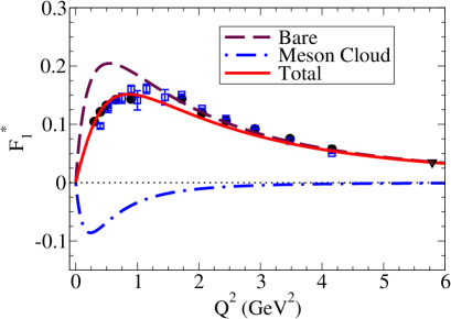
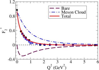
Figure 1: $\gamma^{\ast}N\to N(1535)$ transition form factors for proton target. Data from CLAS CLAS1 , (circles) MAID MAID1 (squares), and JLab/Hall C Dalton09 (triangles). The data at $Q^{2}=0$ is from PDG PDG .

         

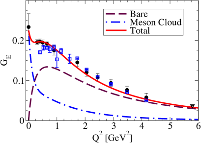
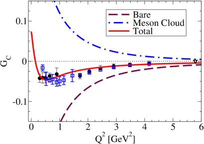
Figure 2: $\gamma^{\ast}N\to N(1535)$ transition form factors $G_{E}$ and $G_{C}$ for proton target. Data from CLAS CLAS1 , (circles) MAID MAID1 (squares), and JLab/Hall C Dalton09 (triangles). The data at $Q^{2}=0$ is from PDG PDG .

	$A_{1/2}(0)$	$F_{2}^{\ast}(0)$	$A(0),B(0)$
$p$	0.105$\pm$0.015	0.97$\pm$0.14	0.14$\pm$0.12
$n$	$-0.075\pm$0.020	$-0.69\pm$0.19	0.83$\pm$0.12

Table 1: Amplitude $A_{1/2}(0)$ and results for $F_{2}^{\ast}(0)$ for the $\gamma^{\ast}N\to N(1535)$ transition. $A_{1/2}(0)$ is in units GeV^-1/2. Data from PDG PDG . In the last column, the first line refers to $A(0)$ and the second line to B(0), defined by Eqs. (27) and (28).

To prepare the following discussion, it is important to notice that $F_{1}^{\ast}(0)=0$ by construction, and that the amplitude $S_{1/2}$ cannot be measured at the photon point since there are no real photons with longitudinal polarization. Therefore, the direct information about the form factors at $Q^{2}=0$ come only from $A_{1/2}$ and $F_{2}^{\ast}$. Those functions are seen to be related at $Q^{2}=0$ by

$$A_{1/2}(0)={\cal C}F_{2}^{\ast}(0),$$ (23)

where ${\cal C}={\cal B}_{0}\eta$ where ${\cal B}_{0}$ is the value of ${\cal B}$, defined in Eq. (6) at $Q^{2}=0$. One obtains then ${\cal C}=\frac{e}{2}\frac{M_{R}-M_{N}}{\sqrt{M_{N}M_{R}K}}$. A summary of the $A_{1/2}$ and $F_{2}^{\ast}$ data at $Q^{2}=0$ is presented in Table 1.

Having in mind that at low $Q^{2}$ the meson cloud excitations are important, we decompose the transition form factors into a bare term (labeled with superscript $\rm B$) and a meson cloud term (labeled with superscript $\rm mc$):

$$F_{1}^{\ast}=F_{1}^{\rm B}+F_{1}^{\rm mc},$$ (24)

$$F_{2}^{\ast}=F_{2}^{\rm B}+F_{2}^{\rm mc},$$ (25)

where the bare contributions are determined by Eqs. (20)–(21) of the covariant spectator quark model in the semirelativistic approximation. The meson cloud terms $F_{1}^{\rm mc}$ and $F_{2}^{\rm mc}$ are to be extracted indirectly from the data.

     

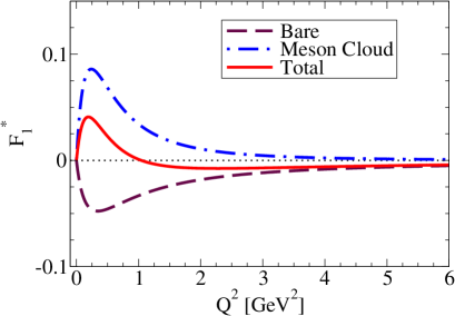
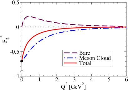
Figure 3: $\gamma^{\ast}N\to N(1535)$ transition form factors for neutron target. The data are from PDG PDG .

     

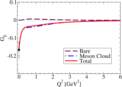
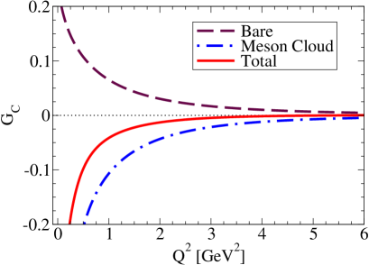
Figure 4: $\gamma^{\ast}N\to N(1535)$ transition form factors $G_{E}$ and $G_{C}$ for neutron target. The data are from PDG PDG .

We start our discussion with $F_{2}^{\ast}$. Since $F_{2}^{\rm mc}$ is a function of $Q^{2}$, we can use the general decomposition

$$F_{2}^{\rm mc}(Q^{2})=A(Q^{2})+B(Q^{2})\,\tau_{3},$$ (26)

where $A$ represent the isoscalar contribution and $B$ represent the isovector contribution. Note that, we cannot parametrize the functions $A$ and $B$ simultaneously because the empirical data for finite $Q^{2}$ are restricted to proton targets. Only for $Q^{2}=0$, there are data for neutron targets. In the last case then we can extract the contributions for $A$ and $B$ using

$$A(0)=\frac{1}{2{\cal C}}[A_{1/2}^{p}(0)+A_{1/2}^{n}(0)],$$ (27)

$$B(0)=\frac{1}{2{\cal C}}[A_{1/2}^{p}(0)-A_{1/2}^{n}(0)].$$ (28)

The results of $A(0)$ and $B(0)$ extracted from the experimental data for $A_{1/2}^{p,n}(0)$ for proton and neutron targets are presented in Table 1.

We conclude from Table 1 that the isovector component dominates, near $Q^{2}=0$, since $B(0)\gg A(0)$. Although the results from Table 1 suggest that $A(0)$ is almost compatible with zero, consistent with the isovector dominance of the meson cloud contribution, the upper limit of $A(0)$, could also be as large as about 1/4 of $B$. This is why we include the isoscalar term $A$ in our parametrization of the meson cloud.

We now discuss the function $F_{1}^{\ast}$. Since $F_{1}^{\ast}(0)=0$ and the bare contribution also vanishes at $Q^{2}=0$, we conclude that the meson cloud contribution should also vanish at $Q^{2}=0$. From the difference between the data and the valence quark contributions (dashed-line) in Fig. 1, we infer that the meson cloud contributions for $F_{1}^{\ast}$ can be significant, below $Q^{2}=1$ GeV². Those contributions are important to the amplitude $A_{1/2}$ (proportional to $G_{E})$ which dominates the structure of the resonances at small $q^{2}$ in the timelike region, as discussed in Sec. V. To parametrize the meson cloud contribution to $F_{1}^{\ast}$, we consider the form

$$F_{1}^{\rm mc}(Q^{2})=C(Q^{2})\;\tau_{3},$$ (29)

where $C$ is a function proportional to $Q^{2}$, near $Q^{2}=0$. With this parametrization, we assume the isovector character of the meson cloud term, motivated by the evidence of the isovector dominance in the amplitude $A_{1/2}$ at $Q^{2}=0$ seen in Table 1. However, the isovector character of $F_{1}^{\rm mc}$ cannot be tested with the present data, since $F_{1}^{\rm mc}=0$ at $Q^{2}=0$, and there are at the moment no available data for the amplitude $A_{1/2}$ with neutron targets, for nonzero $Q^{2}$. Our description of $F_{1}^{\rm mc}$ is then based on an ansatz that can only be tested in the future, once helicity amplitude data for the neutron for finite $Q^{2}$ became also available.

In summary, we can parametrize the meson cloud contributions to the form factors $F_{1}^{\ast}$ and $F_{2}^{\ast}$ using three functions ($A$, $B$ and $C$). The parametrization of $F_{2}^{\rm mc}$ near $Q^{2}=0$ is fixed by the experimental results for the amplitudes $A_{1/2}^{p,n}(0)$, while the general $Q^{2}$-dependence is determined only by the combination $A+B$ (proton target), since there are no data yet for $A-B$ (neutron targets) for finite $Q^{2}$.

The available data support the dominance of the isovector component of the meson cloud on the form factors $F_{1}^{\ast}$ and $F_{2}^{\ast}$. This effect can be observed in the results for the proton targets (Fig. 1) and neutron targets (Fig. 3), where one can notice that the combination of the bare contributions with the meson cloud contributions (solid-lines) based on the isovector dominance provide a good description of the data. Recall that also calculations based on light front relativistic quark models Aznauryan17 conclude that the meson cloud contributions to both Dirac and Pauli form factors are dominated by the isovector component.

To define a parametrization of the meson cloud effects, we have looked at the possible decays of the $N(1535)$ state. There are two main channels for these decays, the $\pi N$ channel and the $\eta N$ channel with about 50% contribution from each component. Minor contributions came from $\pi\Delta$, $\sigma N$ and $\pi N(1440)$. We ignore these last contributions, since the combined effect of those channels is at most 14% PDG . We can then assume that the electromagnetic interaction with the meson cloud is dominated by the $\pi N$ and the $\eta N$ states. Since the $\eta$ meson has no charge, we conclude that the $\eta N$ states contribute to the isoscalar component of the meson cloud, and therefore to the function $A$, while the $\pi N$ states contribute to the isovector component of the meson cloud, and therefore to the function $B$.

For the isoscalar component, we take a parametrization of the form $A\propto F_{\eta}$, where $F_{\eta}$ is the $\eta$ electromagnetic form factor and the additional factors is a multipole type function with a phenomenological cutoff. Since $F_{\eta}$ is not known, we consider the simplest case where all the structure is simulated by a single multipole function,

$$A(Q^{2})=A(0)\left(\frac{\Lambda_{A}^{2}}{\Lambda_{A}^{2}+Q^{2}}\right)^{5},$$ (30)

and where $\Lambda_{A}$ is a cutoff parameter. Importantly, this choice was made to be consistent with perturbative QCD (pQCD) estimates where for very large $Q^{2}$, one has $A\propto 1/Q^{10}$ Carlson .

As for the isovector component, the coupling with the $\pi N$ states is in first approximation determined by the photon coupling with the pion, which is given by the pion electromagnetic form factor $F_{\pi}$. Then one expects that the function $B$ in Eq. (26) to have the form

$$B(Q^{2})\propto F_{\pi}(Q^{2}).$$

The omitted multiplicative functions in this relation are structure functions that determine the extension of the nucleon and resonance cores. One then writes this structure in an effective way as

$$B(Q^{2})=B(0)\left(\frac{\Lambda_{B}^{2}}{\Lambda_{B}^{2}+Q^{2}}\right)^{4}(1+c\,Q^{2})F_{\pi}(Q^{2}),$$

(31)

where the $\Lambda_{B}$ is a short-range (large $Q^{2}$) regulator and $c$ is an adjustable coefficient. The factor $(1+c\,Q^{2})$ was included to improve the quality of the fit by smoothening the variation with $Q^{2}$ in the low-$Q^{2}$ region: a multipole function alone is incompatible with a smooth behavior near $Q^{2}=0$ for $F_{2}^{\ast}$ and $G_{E}$. The power of the multipole function is chosen in order to mimic the falloff of pQCD at very large $Q^{2}$. In a model with $F_{\pi}\propto 1/(Q^{2}\log Q^{2})$, as the one that we consider here, we obtain then $B\propto 1/(Q^{8}\log Q^{2})$, close $1/Q^{10}$, expected from pQCD. Note, however, that for the purpose of the present study, the exact power of the multipole in Eq. (31), (power 3 or 4), is not very relevant, since $\Lambda_{B}^{2}$ only cuts the large the momentum $Q^{2}$ region, and the behavior of $F_{2}^{\rm mc}$ is more sensitive to the low-$Q^{2}$ scale included in $F_{\pi}(Q^{2})$.

To describe $F_{1}^{\rm mc}$, we consider the parametrization

$$C(Q^{2})=-C_{0}\frac{Q^{2}}{\Lambda_{C}^{2}}\left(\frac{\Lambda_{C}^{2}}{\Lambda_{C}^{2}+Q^{2}}\right)^{3}F_{\pi}(Q^{2}),$$ (32)

where $C_{0}$ is a positive constant, and $\Lambda_{C}$ is an adjustable cutoff. At large $Q^{2}$, $F_{1}^{\rm mc}$ goes with $1/(Q^{6}\log Q^{2})$, closer to the falloff $1/Q^{8}$ estimated by pQCD. The factor $F_{\pi}$ is included due to the isovector form associated with $F_{1}^{\rm mc}$ discussed before.

For $F_{\pi}$ we use the parametrization already tested in the case of the $\Delta(1232)$ Timelike2

$$F_{\pi}(Q^{2}) = \frac{\alpha}{\alpha+Q^{2}+\frac{1}{\pi}\beta Q^{2}\log\frac{Q^{2}}{m_{\pi}^{2}}},$$ (33)

$$= \frac{\alpha}{\alpha-q^{2}-\frac{1}{\pi}\beta q^{2}\log\frac{q^{2}}{m_{\pi}^{2}}+i\beta q^{2}},$$

where $\alpha=0.696$ GeV², $\beta=0.178$, and $m_{\pi}$ is the pion mass.

The previous parametrization was derived in Ref. Timelike2 based on analytic expressions that take into account the effects of the pion loop contributions to the $\rho$-meson propagator. The original form Iachello ; Iachello73 ; Frohlich10 included the effect of the two-pion threshold expressed by a dependence on $(q^{2}-4m_{\pi}^{2})$. We consider the approximation $q^{2}\gg 4m_{\pi}^{2}$ and obtain a smoother description of the imaginary components without loss of accuracy Timelike ; Timelike2 .

III.5 Combination of valence quark and meson cloud contributions

The parameters of meson cloud contributions to the transition form factors $F_{1}^{\ast}$ and $F_{2}^{\ast}$ can be determined by the fit of the parameters of the expressions (30), (31) and (32), to the $F_{1}^{\ast}$ and $F_{2}^{\ast}$ form factor data for proton targets, and the $F_{2}^{\ast}(0)$ data for neutron targets. An alternative, is to fit those parametrizations directly to the form factors $G_{E}$ and $G_{C}$.

We choose the second option for two main reasons: our final goal is to derive parametrizations for the multipole form factors in the timelike region; the $F_{1}^{\ast}$ and $F_{2}^{\ast}$ data are represented by very sharp functions near $Q^{2}=0$. By contrast the form factors $G_{E}$ and $G_{C}$ have a softer shape at low $Q^{2}$.

In the fit, we considered an additional constraint: we imposed that the ratio $A(Q^{2})/B(Q^{2})$ should not increase in the region of study ($Q^{2}<5$ GeV²) in order to be consistent with the isovector dominance observed at the photon point ($Q^{2}=0$), and supported by independent calculations Aznauryan17 .

$A(0)$	0.125
$\Lambda_{A}^{2}$ (GeV2)	2.384
$B(0)$	0.810
$c$ (GeV-2)	2.040
$\Lambda_{B}^{2}$ (GeV2)	3.365
$C_{0}$	0.873
$\Lambda_{C}^{2}$ (GeV2)	0.785

Table 2: Parameters of the meson cloud parametrizations. The numerical results for the functions $A$, $B$ and $C$ are presented in Fig. 6.

The parameters associated for the best fit to $G_{E}$ and $G_{C}$ with the described constrains are displayed in Table 2. In the following, we represent the meson cloud contributions associated with the fit by the dashed-dotted-lines. The valence quark (bare) contributions are represented by dashed-lines. The result of the combination of the valence quark and the meson cloud contributions is represented in the same graph by the solid-lines. We start our discussion with the results for proton targets. The final results for the $F_{1}^{\ast}$ and $F_{2}^{\ast}$ form factors for proton target are presented in Fig. 1. The corresponding results for $G_{E}$ and $G_{C}$ are presented in Fig. 2.

In the figures, one notices a sharp variation of the functions $G_{E}$ and $G_{C}$ at low $Q^{2}$, more particularly in the range $Q^{2}=0$–0.3 GeV². Those results are a consequence of the fit to the low-$Q^{2}$ data and of the lack of data in the region $Q^{2}=0$–0.3 GeV². New data in that region are necessary for more definitive conclusions relative to the shape of $G_{E}$ and $G_{C}$ at low $Q^{2}$ Compton ; Siegert4 . It is interesting to notice, however, that the shape of $G_{C}$ near $Q^{2}=0$ is similar to the shape estimated with the constraints from Siegert’s theorem Siegert1 ; Compton .

The results of the form factors for neutron targets are presented in Figs. 3 and 4. From the figures, we can conclude that the magnitudes of the $F_{1}^{\ast}$ and $F_{2}^{\ast}$ are smaller than those for proton target. As for the $G_{E}$ form factor it is interesting to notice that $G_{E}$ is very small (except for $Q^{2}<0.25$ GeV²) as a consequence of the cancellation between valence quark and meson cloud contributions for the neutron case. As for $G_{C}$, one notices that it is larger in magnitude than in the case of the proton, as the consequence a less significant cancellation between valence quark and meson cloud contributions.

Our result of $G_{C}$ for the proton target at low $Q^{2}$ (Fig. 2) requires some extra discussion. In the graph the function changes sign, when $Q^{2}$ approaches the photon point. But due to the lack of data below $Q^{2}=0.3$ GeV², we cannot say that this change of sign is imposed by the data. Other parametrizations suggest that $G_{C}$ is small near $Q^{2}=0$ MAID1 ; Compton ; Siegert4 , but the present data are unable to determine the exact sign. In our model, the magnitude of $G_{C}$ near $Q^{2}=0$ is related to the regularization of the form factors $F_{i}^{\ast}(Q^{2})$, specifically the factor $\sqrt{\frac{Q^{2}}{\Lambda_{R}^{2}+Q^{2}}}$ from Eq. (22). In appendix B, we explicitly demonstrate this by decomposing $G_{C}(0)$ into three terms, two positive in sign, associated with $F_{2}^{\ast}(0)$ and with the meson cloud contribution to $F_{1}^{\ast}$, and one negative, proportional to $1/\Lambda_{R}^{2}$. Then, a small value for $\Lambda_{R}$, leads to a large cancellation of terms and a small value for $G_{C}(0)$. A larger value for $\Lambda_{R}$, like $\Lambda_{R}=m_{\rho}$, reduces the magnitude of that cancellation and increases the value of $G_{C}(0)$. In summary, the value for $G_{C}(0)$ is a consequence of the value $\Lambda_{R}$ chosen to estimate the bare contribution of the transition form factors, and it is not well constrained by the data.

On the other hand, the combined fit to the proton and neutron data for $G_{E}(0)$ is weakly dependent on the parameter $B(0)$. This is a consequence of the small error bars of the $F_{2}^{\ast}$ data for the proton, for finite $Q^{2}$, and the large error bars at $Q^{2}=0$ of the data for the proton and neutron (PDG data). For that reason the finite $Q^{2}$ points have a stronger impact on the fit, leaving less room for the much less constrained data at $Q^{2}=0$.

To exhibit the control on the uniqueness of the parameters obtained in the fitting procedure we show in Fig. 5 the results of $F_{2}^{\rm mc}$ for the proton and neutron cases in comparison with their parametrizations by $A+B$ and $A-B$ respectively. The $F_{2}^{\rm mc}$ experimental points are determined by $F_{2}^{\rm mc}=F_{2}^{\ast}-F_{2}^{\rm B}$, where $F_{2}^{\ast}$ is the experimental value and $F_{2}^{\rm B}$ the model result, for both proton and neutron targets (there is a single experimental point for the neutron case).

Those experimental points are included just to guide the eye, since the meson cloud parametrization are determined by the direct fit to the $G_{E}$ and $G_{C}$ data. If we neglect the isoscalar component, we obtain $F_{2n}^{\rm mc}=-F_{2p}^{\rm mc}$, or in other words, the difference between the red and blue curves of Fig. 5 is due to that component alone.

Figure 5 shows also that increasing or decreasing the estimate for $F_{2n}^{\rm mc}$ by about 0.05 (one third of the error bar) the result for $F_{2n}^{\rm mc}(0)$, is still consistent with its experimental limits. This result shows, that $B(0)$ can vary within a certain range without changing the results for $F_{2p}^{\rm mc}$ provided that the value for $A(0)$ is redefined in order to keep the result for $F_{2p}^{\rm mc}(0)\simeq 0.97$ (estimated based on experimental data, Table 1). In summary, we obtain a solid estimate for the proton data, but a poorer estimate of the neutron data. This happens because the neutron data is constrained only by one data point ($Q^{2}=0$) with a large error bar.

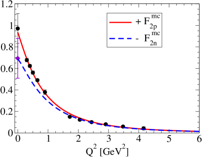
Figure 5: Data estimate of the functions $F_{2p}^{\rm mc}$ (circles) and $-F_{2n}^{\rm mc}$ (diamond) for the $\gamma^{\ast}N\to N(1535)$ transition.

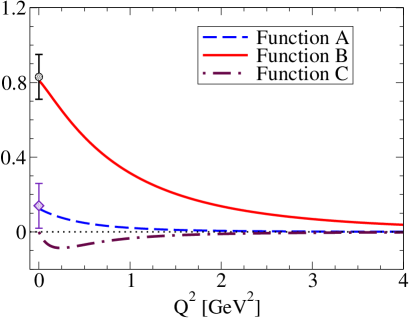
Figure 6: $\gamma^{\ast}N\to N(1535)$ transition: functions $A$, $B$ and $C$ used to parametrize the meson cloud contributions to the transition form factors $F_{1}^{\rm mc}$ and $F_{2}^{\rm mc}$.

We represent separately in Fig. 6, the functions $A$, $B$ and $C$, parametrizing the meson cloud effects. In the case of the functions $A$ and $B$, we include also their experimental limits at $Q^{2}=0$ presented in Table 1. We recall that i) by construction, and to enforce the isovector dominance for larger values of $Q^{2}$ the ratio $A/B$ is smaller than the ratio at $Q^{2}=0$ (about $0.15/0.82\approx 0.2$); ii) there are no experimental constraints except for $C(0)=0$.

We emphasize that the isovector character of $F_{1}^{\rm mc}$, from Eq. (29) is an ansatz. No empirical information is available at the moment that allows us to test this assumption.

From the study of the proton and neutron form factors, we conclude that is possible to obtain an accurate description of the proton target data. The results for the neutron target, however, are poorly constrained. More precise calculations of the transition form factors with neutron targets are possible only with more accurate constraints from the neutron sector.

It is worth mentioning, that we can obtain almost equivalent descriptions of the proton and neutron target data with a small modification of the parameter $A(0)$, provided that $B(0)$, is readjusted such that $B(0)\simeq[F_{2p}^{\ast}(0)]_{\rm exp}-A(0)$ holds, and keeping all the remaining parameters unchanged. The results for the proton target remain almost unchanged and the results for $F_{2}^{\ast}$ for the neutron target are modified according with the new values for $A(0)$ and $B(0)$. This property may be very useful in future works, allowing us to investigate the sensitivity of the neutron transition form factors for different classes of parametrizations characterized by different $A(0)$.

III.6 Summary of the results in the spacelike region

Combining the parametrizations of the meson cloud contribution with results from the valence quark contribution from the covariant spectator quark model we obtain a good description of the proton target data for $G_{E}$ and $G_{C}$ and at the same time a good description of the form factors $F_{1}^{\ast}$ and $F_{2}^{\ast}$ in the spacelike region. Also, we have identified the isoscalar and isovector the contributions, based on the Pauli-Dirac representation, in a model that accounts for transitions both with proton and neutron targets.

Next, in the extension of their results to the timelike region, we will focus on the form factors $G_{E}$ and $G_{C}$, since timelike formulas for decay widths are more readily expressed in terms of those form factors.

         

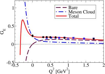
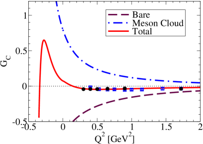
Figure 7: Real part of $\gamma^{\ast}N\to N(1535)$ transition form factors in the spacelike and timelike region, for proton target for $W=1.535$ GeV. Same data as in Fig. 1.

     

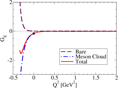
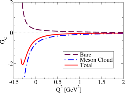
Figure 8: Real part of $\gamma^{\ast}N\to N(1535)$ transition form factors in the spacelike and timelike region, for neutron target for $W=1.535$ GeV. The data at $Q^{2}=0$ is from PDG PDG .

         

         

         

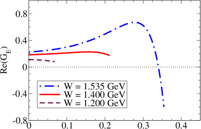
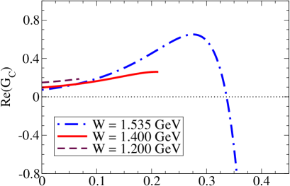
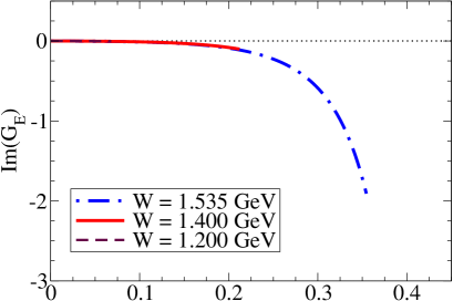
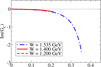
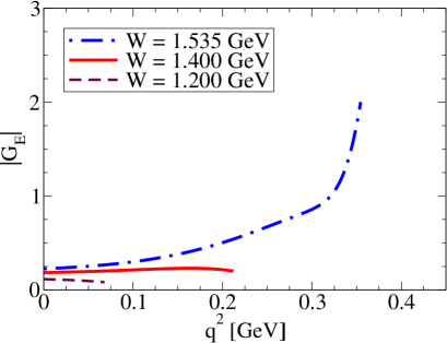
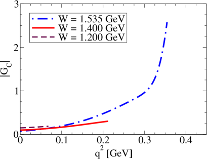
Figure 9: $\gamma^{\ast}N\to N(1535)$ transition form factors for proton target for different values of $W$.

         

         

         

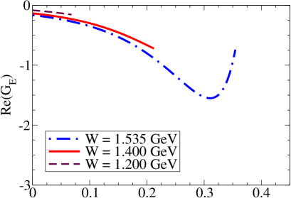
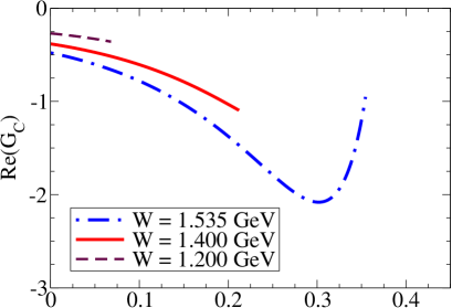
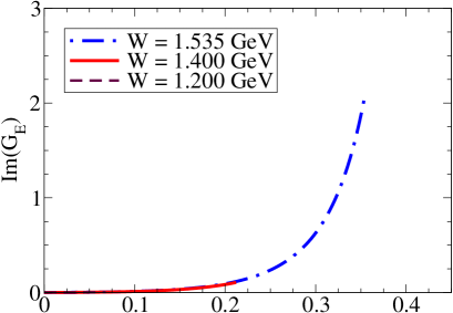
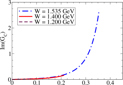
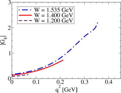
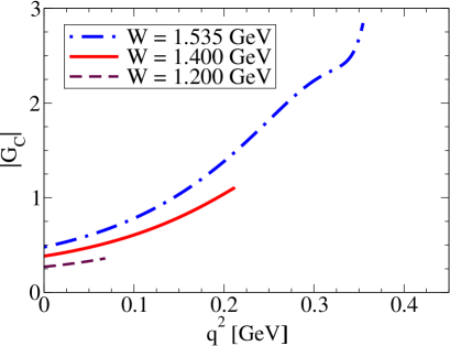
Figure 10: $\gamma^{\ast}N\to N(1535)$ transition form factors for neutron target for different values of $W$.

         

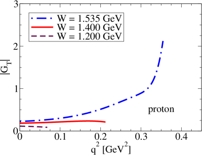
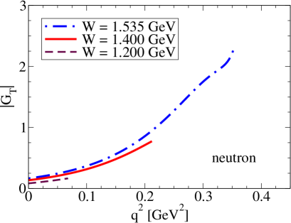
Figure 11: Effective form factor function $|G_{T}|$ for different values of $W$. Comparison between proton and neutron results.

IV Extension to the timelike region

We describe now how the extension of the model from the spacelike region for the timelike region. In the timelike region, we vary the energy $W$ of the $\gamma^{\ast}N$ system, which may differ from the $N(1535)$ resonance mass ($M_{R}$). In transforming the spacelike formulas to the timelike region we then replace $M_{R}$ by $W$. As done in the spacelike region, we decompose the form factors into the bare and meson cloud contributions, according to Eqs. (24)–(25).

A note about the range of application of our framework is in order. We are aiming at the region of $W$ accessible in the present day experiments, in particular the range of $W$ probed at HADES, which is restricted to typical values of $W\simeq 1.490$ GeV HADES17a ; HADES17b . Since, according to the kinematic relations (3) and (4), the values of $q^{2}$ are restricted to $q^{2}\leq(W-M_{N})^{2}$, one concludes that the square invariant moment of the dilepton are limited to $q^{2}\leq 0.3$ GeV².

The formalism described in the present work for the valence quark component of the model is constrained by the scale $\Lambda_{R}=m_{\rho}$ and therefore restricted to the upper limit $W=M_{N}+m_{\rho}\simeq 1.7$ GeV. The numerical approximations discussed below, however, are also limited to not very large values for $q^{2}$, reducing the range of application of $W$ to the order 1.6 GeV, still within the window covered by the HADES experiments. In comparison with other resonances described by the covariant spectator quark model, $\Delta(1232)$ and $N(1520)$ Timelike ; Timelike2 ; N1520TL , the $N(1535)$ resonance is the one lying closer to the $\rho$-pole. Thus, for large $W$, there is the possibility of enhancement of the transition form factors.

IV.1 Valence quark contributions

In the present work, we use the timelike extension of the quark electromagnetic form factors of the covariant spectator quark model defined by the study of the $\gamma^{\ast}N\to N(1520)$ transition in the timelike region N1520TL . Note that differently to the $\gamma^{\ast}N\to\Delta(1232)$ transitions the $\gamma^{\ast}N\to N(1535)$ and $\gamma^{\ast}N\to N(1520)$ transitions require isovector and isoscalar components.

The extension to timelike of the valence quark contributions is based on the analytic expressions for $F_{1}^{\rm B}$ and $F_{2}^{\rm B}$ in the spacelike region, given by Eqs. (20)–(21). In those expressions we convert $Q^{2}\to-q^{2}$, and replace the physical mass $M_{R}$ by $W$.

One can factorize the bare form factors (20)–(21) into two leading factors: One first factor includes all the functions $j_{i}^{A,S}$ ($i=1,2$) comprising the quark form factors, according to Eqs. (14)–(15). There, the quark isoscalar and isovector form factors contain the vector meson poles, including the mesons $\rho$ and $\omega$, and are then naturally defined in the timelike region with the introduction of $q^{2}$-dependent widths.

The other factor is the product of $Z$ from Eq. (22) and the integral ${\cal I}_{R}$ over the radial wave functions in Eq. (16), and reads

$${\cal I}_{R}^{\prime}={\cal I}_{R}\sqrt{\frac{Q^{2}}{m_{\rho}^{2}+Q^{2}}}.$$ (34)

Remember that, as discussed in the context of the semirelativistic approximation, the overlap integral ${\cal I}_{R}$ of Eq. (16) cannot be evaluated below $Q^{2}=0$ because the region $-(W-M_{N})^{2}\leq Q^{2}<0$ cannot be accessed. One can, however, use a numerical extrapolation of the results in the spacelike region to the timelike region, using an analytic continuation for $Q^{2}<0$.

The analytic continuation of ${\cal I}_{R}$ is based on the observation that the in the spacelike region the function ${\cal I}_{R}/|{\bf q}|$ is well described by a dipole form for small values of $Q^{2}$. One uses then the replacement:

$$\frac{{\cal I}_{R}}{|{\bf q}|}\to\frac{G_{D}(q^{2})}{M_{N}},$$ (35)

where $G_{D}$ is a dipole function with $G_{D}(0)$ and a cutoff $\Lambda_{D}$ determined by the values of $Q^{2}$ close to $Q^{2}=0$. The details of this procedure are presented in Appendix C.

Combining the analytic extension of the two factors from Eq. (34), we obtain (see Appendix C):

$${\cal I}_{R}^{\prime}\simeq-\frac{q^{2}G_{D}(q^{2})}{M_{N}(W+M_{N})}\sqrt{\frac{(W+M_{N})^{2}-q^{2}}{m_{\rho}^{2}-q^{2}}}.$$ (36)

It is worth noticing that this analytic extrapolation is not free of uncertainties and that specially an extension for very large values of $q^{2}$ may not be very accurate. Nonetheless, since we are restricted to $q^{2}\leq(W-M_{N})^{2}$, the approximation is justified as far as we restrict our study to not very large values for $W$. For $W=1.535$ GeV, we obtain at most $q^{2}\simeq 0.35$ GeV² or $\sqrt{q^{2}}\simeq 0.6$ GeV.

The singularities presented on (36), one associated to the dipole factor, and another with the $\rho$-pole, can be regularized: to each regulating scale $\Lambda$ ($\Lambda_{D}$ or $m_{\rho}$) we associate finite width $\Gamma_{\Lambda}$. For a given power of $n$ (integer) we then use the replacement

$$\left(\frac{\Lambda^{2}}{\Lambda^{2}-q^{2}}\right)^{n}\to\left(\frac{\Lambda^{4}}{(\Lambda^{2}-q^{2})^{2}+\Lambda^{2}[\Gamma_{\Lambda}(q^{2})]^{2}}\right)^{\frac{n}{2}}.$$ (37)

This way, we consider the absolute value of the multipole. The same method was used in previous works N1520TL ; Timelike2 . The explicit expression for the effective width $\Gamma_{\Lambda}(q^{2})$ is presented in Appendix D. In the case of ${\cal I}_{R}^{\prime}$ in Eq. (36), we extend the previous expression to half-integers, $n=\frac{1}{2}$. With the procedure (37), we simplify the expressions in the timelike region.

IV.2 Meson cloud contributions

The extension of the meson cloud component to the timelike region is straightforwardly based on Eqs. (26)–(32). The parametrizations of the meson cloud contributions are determined by the calibration of the form factors $F_{1}^{\ast}$ and $F_{2}^{\ast}$ at the physical mass ($W=M_{R}$). Although the meson cloud parametrizations for $F_{1}^{\ast}$ and $F_{2}^{\ast}$ are independent of $W$, since the calculations $G_{E}$ and $G_{C}$ are done through Eqs. (7) and (8) where the coefficients now depend on $W$, the meson cloud contributions for those form factors depend on $W$.

The relations (26)–(32) used in the parametrizations of the meson cloud contributions are automatically converted to the timelike region with the replacement $Q^{2}\to-q^{2}$. To regularize the multipole functions we use the procedure from Eq. (37). In the pion form factor $F_{\pi}(q^{2})$ the imaginary component is generated naturally for $q^{2}>0$ (see Eq. (33)). Due to the magnitude of the regulators presented on Eqs. (30), (31) and (32) only the the function $C$, given by Eq. (32) requires in fact the use of the regularization (37), because $\Lambda_{C}^{2}\simeq 0.785$ GeV² is closer to the region of study $q^{2}=(M_{R}-M_{N})^{2}\simeq 0.36$ GeV².

IV.3 $\gamma^{\ast}N\to N(1535)$ form factors in the timelike region

We present now the results in the timelike region for the form factors $G_{E}$ and $G_{C}$. We start with the results for the case $W=M_{R}$ that expand Figs. 2 and 4 into the region $-(M_{R}-M_{N})^{2}\leq Q^{2}\leq 0$. Later on, we study the dependence of the form factors (real and imaginary parts) for several values of $W$.

The results in the timelike region are presented in Fig. 7 for proton targets and in Fig. 8 for neutron targets. Although the transition form factors became complex in the timelike region, in the figures, for now, we show only the real part of the form factors in order to be able to compare the results directly with the physical spacelike data.

The results from Fig. 7 (proton target) indicate that the real part of $G_{E}$ changes sign below $Q^{2}=0$. This is a consequence of the combination $F_{1}^{\ast}$ and $F_{2}^{\ast}$ and may have been anticipated from the results from Fig. 1: since those functions have opposite sign below $Q^{2}=0$, then $G_{E}=F_{1}^{\ast}+\eta F_{2}^{\ast}$ may vanish at some point below $Q^{2}=0$. Notice that $F_{1}^{\ast}$ and $F_{2}^{\ast}$ are both finite at the pseudothreshold Siegert1 . The zero in the real part of $G_{C}$ then occurs as a consequence of the constraint from Siegert’s theorem, which states that $G_{C}\propto G_{E}$ near the pseudothreshold. More details can be found in Appendix A.

The results for the real part of the transition form factors for neutron targets in Fig. 8 show a significant enhancement of the bare and meson cloud contributions below $Q^{2}=0$ for both form factors. Recall that the value of $G_{E}$ at $Q^{2}=0$ is the only physical constraint used in the model parametrization. The results for neutron target are then the result of the extrapolation of our model parametrization to the valence quark contribution and our phenomenologically motivated parametrization of the meson cloud effects. Concerning the final result (solid-line) for $G_{E}$ and $G_{C}$, the negative bump observed in both functions is the consequence of two main effects: the enhancement of the function ${\cal I}_{R}$ due to the dipole shape, and the vicinity the $\rho$-meson pole which suppresses the real part of the form factors, and is present on both the bare and meson cloud components (since $F_{\pi}$ peaks near $q^{2}\approx m_{\rho}^{2}$).

The results for the form factors for the values $W=1.2$, 1.4 and 1.535 GeV are presented in Figs. 9 and 10 for proton and neutron targets, respectively. The upper value of $q^{2}$ for each value of the energy resonance energy $W$ corresponds to the pseudothreshold point $q^{2}=(W-M_{N})^{2}$. The figures show both the real part (upper panel) and the imaginary part (middle panel), and present also the results for the absolute values $|G_{E}|$ and $|G_{C}|$ (lower panel). For convenience, we present the results only for the timelike region, i.e. $q^{2}>0$.

In Figs. 9 and 10 the results near the pseudothreshold, $q^{2}=(W-M_{N})^{2}$, are modified compared to a model which ignores the regularization of the singularities (poles $\Lambda_{D}^{2}$, $m_{\rho}^{2}$, $\Lambda_{C}^{2}$, etc.). In general, the regularization reduces the magnitude of the form factors in the vicinity of the pseudothreshold. We can anticipate here that although the effective results for the real and imaginary parts of the form factors depend on the regularization, in particular on the width associated with the dipole function in Eq. (35), the final results for the $N(1535)$ Dalitz decay widths (integrated in $q$), presented in Sec. VI, have a very weak dependence on the regularization parameters.

From the previous figures, one can conclude that $G_{E}$ and $G_{C}$ have similar magnitudes for their real and imaginary components. The relevant function for the timelike calculations, discussed in the next section, is, however, the effective form factor defined by the combination of $|G_{E}|^{2}$ and $|G_{C}|^{2}$

$$|G_{T}(q^{2},W)|^{2}=|G_{E}(q^{2},W)|^{2}+\frac{q^{2}}{2W^{2}}|G_{C}(q^{2},W)|^{2},$$

(38)

where the form factors $G_{E}$ and $G_{C}$ are defined by Eqs. (7)–(8), with the replacement $M_{R}\to W$.

Notice in Eq. (38) that the contribution of $|G_{C}|$ is suppressed at low $q^{2}$ by the factor $q^{2}/(2W^{2})$. One expects then that $|G_{C}|$ becomes relevant only for large $q^{2}$ values, corresponding also to large values of $W$, since $q^{2}\leq(W-M_{N})^{2}$.

The results for the form factor $|G_{T}|$ for the values $W=1.2$, 1.4 and 1.535 GeV are presented in Fig. 11 for proton and neutron targets. Note that the magnitude of $|G_{T}|$ becomes larger for neutron targets when $q^{2}>0.1$ GeV². In both channels the dominant effect comes from the electric form factor. The contribution of the Coulomb form factors increases the function $|G_{T}|$ in 10% at most.

In the next section we present the formalism associated with the $N(1535)$ Dalitz decay. In Sec. VI we use our results for $|G_{T}|$ to calculate the Dalitz decay functions.

V $N(1535)$ Dalitz decay

We discuss now the formalism associated with the $N(1535)$ Dalitz decay ($N^{\ast}\to e^{+}e^{-}N$). As in the previous section, $W$ represent the mass of the resonance.

Our starting point is the calculation of the function $\Gamma_{\gamma^{\ast}N}(q,W)$, which determine the decay width of state with mass $W$ into a photon with virtuality $q^{2}>0$. The variable $q$ is then defined by $q=\sqrt{q^{2}}$.

The function $\Gamma_{\gamma^{\ast}N}(q,W)$ is defined according to Ref. Krivoruchenko02

$$\Gamma_{\gamma^{\ast}N}(q,W)=\frac{\alpha}{2W^{3}}\sqrt{y_{+}y_{-}}y_{+}|G_{T}(q^{2},W)|^{2},$$

(39)

where $|G_{T}(q^{2},W)|$ is defined by Eq. (38) and

$$y_{\pm}=(W\pm M_{N})^{2}-q^{2}.$$ (40)

From Eq. (39) one concludes that the impact of the form factors in the Dalitz decay functions is determined by the function $|G_{T}|$, given by Eq. (38).

Once the function $\Gamma_{\gamma^{\ast}N}(q,W)$ is defined, one can calculate the dilepton decay rate using the derivative Krivoruchenko02

$$\Gamma^{\prime}_{e^{+}e^{-}N}(q,W) \equiv \frac{d\Gamma_{e^{+}e^{-}N}}{dq}(q,W)$$

$$= \frac{2\alpha}{3\pi q^{3}}(2\mu^{2}+q^{2})\sqrt{1-\frac{4\mu^{2}}{q^{2}}}\Gamma_{\gamma^{\ast}N}(q,W),$$

where $\mu$ is the electron mass.

The Dalitz decay width can then be determined by the integral of $\Gamma^{\prime}_{e^{+}e^{-}N}(q,W)$ in the region $4\mu^{2}\leq q^{2}\leq(W-M_{N})^{2}$:

$$\Gamma_{e^{+}e^{-}N}(W)=\int_{2\mu}^{W-M_{N}}\Gamma^{\prime}_{e^{+}e^{-}N}(q,W)\,dq.$$ (42)

The radiative decay, $N^{\ast}\to\gamma N$, is calculated from the function $\Gamma_{\gamma^{\ast}N}(q,W)$, in the limits $q^{2}=0$ and $W=M_{R}$. Using Eq. (39), one obtains

$$\Gamma_{\gamma N}=\frac{\alpha}{M_{R}^{2}}(M_{R}+M_{N})^{2}K|G_{E}(0,M_{R})|^{2}.$$ (43)

The previous result is consistent with the general expression in terms of helicity amplitudes for a resonance with spin $J=\frac{1}{2},\frac{3}{2}$ PDG97 ; Aznauryan12a :

$$\Gamma_{\gamma N}=\frac{2}{(2J+1)\pi}K^{2}\frac{M_{N}}{M_{R}}\left[|A_{1/2}|^{2}+|A_{3/2}|^{2}\right],$$ (44)

where $A_{1/2}$, $A_{3/2}$ represent the transverse helicity amplitudes (at resonance rest frame) for $Q^{2}=0$. As before $K=\frac{M_{R}^{2}-M_{N}^{2}}{2M_{R}}$. In the present case ($J=\frac{1}{2}$), one has $A_{3/2}\equiv 0$.

VI Results for the radiative and Dalitz decay widths

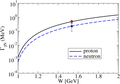
Figure 12: Radiative decay width as function of $W$ for the proton and neutron cases. The data ($W=M_{R}$) are determined from the PDG data for the amplitude $A_{1/2}(0)$.

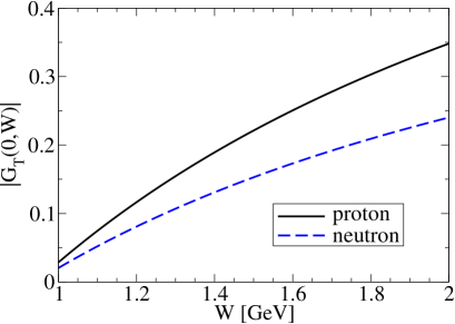
Figure 13: Effective form factor function $|G_{T}(0,W)|$ for the proton and neutron cases.

         

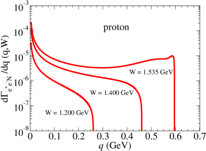
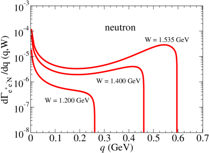
Figure 14: Dilepton decay rates $\frac{d}{dq}\Gamma_{e^{+}e^{-}N}(q,W)$. for the cases $W=1.2$, 1.4 and 1.535 GeV. The upper limit in $q$ is $W-M_{N}$.

We present in this section the observables associated with the timelike region. First, we present our results for the radiative decay widths ($\Gamma_{\gamma N}$). Next we discuss our results for the dilepton decay rates $\frac{d}{dq}\Gamma_{e^{+}e^{-}N}(q,W)$. We also show the results for the Dalitz decay widths ($\Gamma_{e^{+}e^{-}N}$), as function of $W$. We consider the proton and neutron cases.

	$A_{1/2}(0)$ [GeV-1/2]		$\Gamma_{\gamma N}$ [MeV]
	Data	Model	Estimate	PDG limits	Model
$p$	0.105$\pm$0.015	0.101	0.49$\pm$0.14	0.19–0.53	0.503
$n$	$-0.075\pm$0.020	$-0.074$	0.25$\pm$0.13	0.013–0.44	0.240

Table 3: $N(1535)\to\gamma N$ decay widths. Estimate represent the PDG result calculated from the amplitude $A_{1/2}(0)$. PDG limits labels result obtained from the branching ratios.

VI.1 Radiative decay widths

The radiative decay widths for the proton and neutron are determined by the function $\Gamma_{\gamma^{\ast}N}(q,W)$ as defined by Eq. (39) in the limit $q^{2}=0$, when the virtual photon became real.

The results for $\Gamma_{\gamma N}$ are presented in Fig. 12, for the proton and neutron cases. Our results differ significantly from the results of a model with constant form factors.

Notice that the result for $\Gamma_{\gamma N}$ is related to $|G_{T}(0,W)|^{2}$. The results of the function $|G_{T}(0,W)|$ are presented in Fig. 13. From the figure it is clear that the constant form factor, i.e. a $W$ independent form factor, is a bad approximation.

The results for $\Gamma_{\gamma N}(W)$ for the physical point ($W=M_{R}$) compare well with experimental values presented in Table 3. The data presented in Fig. 12 are PDG results based on the amplitudes $A_{1/2}(0)$ (fourth column of Table 3). The uncertainties in the widths are the consequence of limits on $A_{1/2}(0)$ [proportional to $G_{E}(0)$]. Note that there is some overlap between the data results for the proton and neutron, meaning that the data are compatible with an identical result for both decays (exact isospin symmetry).

In our model, the isospin symmetry is clearly broken in the $N(1535)\to\gamma N$ decay. The good agreement between model and data is a consequence of the accurate description of the transition form factor $G_{E}$ at $q^{2}=0$, for both isospin channels.

VI.2 Dalitz decay rates

The dilepton decay rate $\frac{d}{dq}\Gamma_{e^{+}e^{-}N}(q,W)$ can be calculated combining Eq. (LABEL:eqDGamma) with Eq. (39). The results for $W=1.2$, 1.4 and 1.535 GeV are presented in Fig. 14 for the proton (left panel) and neutron (right panel) cases. The upper limit in $q$ is determined by $q=W-M_{N}$, as before.

From Fig. 14, we can conclude that the more relevant kinematic regions, for both channels, is the low-$q$ region or near the pseudothreshold for large $W$, where there is a substantial enhancement of the decay rate. In the figure, one can also notice that the magnitude of the decay rates near $q^{2}=0$ is larger for the proton.

VI.3 Dalitz decay widths

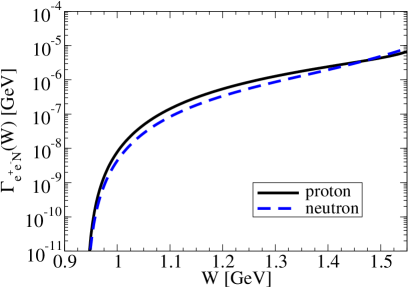
Figure 15: Dalitz decay widths as function of $W$ for the proton and neutron.

The function $\Gamma_{e^{+}e^{-}N}(W)$ is determined by the integral of the dilepton decay rate according to Eq. (42). The results for the proton and neutron cases are presented in Fig. 15.

In the figure we can notice a dominance of the proton decay width up to $W=1.4$ GeV and very close values for proton and neutron cases near $W=1.5$ GeV. Above 1.5 GeV, close to the $\rho$ meson mass pole ($W=M_{N}+m_{\rho}\simeq 1.7$ GeV) the effect of the corresponding pole starts to manifest. The main effect is the enhancement of $\Gamma_{e^{+}e^{-}N}(W)$. We have a glimpse of this effect in the graph for the neutron decay (dashed-line).

The dominance of the Dalitz decay width for proton decay over the results for neutron decay is explained by the dominance of the dilepton decay rates near $q=0$, as can be confirmed by Fig. 14 (right panel versus left panel). For larger values of $q$ (and larger $W$) the magnitude of the neutron dilepton decay rates increases more in comparison to the proton dilepton decay rates (see Fig. 14). When we integrate on $q$ to obtain $\Gamma_{e^{+}e^{-}N}(W)$, the impact of the large $q$ region on the dilepton decay rate is larger, and the neutron Dalitz decay width is enhanced.

Since we aim at the range of the HADES experiments, we do not go beyond $W\simeq 1.55$ GeV. The values of the function $\Gamma_{e^{+}e^{-}N}(W)$, at $W=M_{R}$ are given in Table 4. From the table we can conclude that the results for proton and neutron decays are very close, $\Gamma_{e^{+}e^{-}N}(M_{R})\simeq 6$–7 keV. This result contrasts with what occurs in the radiative decay, $\Gamma_{\gamma N}(M_{R})$, where the widths for the two isospin channels differ much more.

In a model where we reduce the isoscalar component $A(0)$ by in about 0.05, which as discussed in Sec. III.5 ($A(0)\to A(0)-0.05\simeq 0.075$) is still well within the experimental limits, the results for $\Gamma_{e^{+}e^{-}N}(W)$ are almost indistinguishable in the two channels.

The timelike data about the neutron decays is very important because they provide information about the neutron structure which is not available at the moment from spacelike experiments. For this reason pion-induced reactions at HADES ColeTL ; Ramstein18a are fundamental to pin down to electromagnetic structure of the neutron and complement the information from the spacelike region.

In Fig. 16, we compare the $N(1535)$ Dalitz widths with estimates for other light mass resonances, based on the covariant spectator quark model. We show the results for the $\Delta(1232)\frac{3}{2}^{+}$, where the pion cloud contributes with about 45% to the transition form factors at the photon point Timelike2 , and also the results for $N(1520)\frac{3}{2}^{-}$N1520TL .

Figure 16 shows that the $\Delta(1232)\frac{3}{2}^{+}$ dominates within the range of $W$ considered, although the $\Delta(1232)$ Dalitz decay at the pole is measured for smaller values of $W$. The Dalitz decay branching ratio for this resonance is consistent with the value recently extracted from the dilepton production spectrum data HADES17a .

	$\Gamma_{e^{+}e^{-}N}$ (keV)
$p$	5.7
$n$	7.2

Table 4: $N(1535)\to\gamma N$ Dalitz decay widths, estimated by the present model.

VII Outlook and conclusions

Theoretical models for the electromagnetic structure of the $N^{\ast}$ resonances in the timelike region are necessary for the interpretation of $N^{\ast}$ Dalitz decays measured currently in experiments at HADES HADES17a ; HADES-dilepton ; Ramstein18a .

The structure of the $\gamma^{\ast}N\to N(1535)$ transition given by the experimental data for spacelike form factors is non-trivial and suggests that it results from a combination of valence quark and meson cloud effects. Valence quark models describe well the Dirac form factor for $Q^{2}>1.5$ GeV² but they fail to describe the Pauli form factor data. In contrast, chiral models predict important meson cloud contributions to the Pauli form factor in the low-$Q^{2}$ region.

In this work, we developed a model for the $\gamma^{\ast}N\to N(1535)$ transition in the timelike region. The model is based on the covariant spectator quark model in the spacelike region, which is here combined with the semirelativistic approximation that neglects baryon mass difference in the overlap integral of the initial and final state. This approximation guarantees the orthogonality of the initial and final wave functions as well as current conservation. It also enables us to use the same radial wave function for the nucleon and the $N(1535)$. Therefore all the estimates for the valence quark contributions in the spacelike region are true predictions of a parametrization fixed from nucleon elastic form factors. We also modify the behavior of the form factors at low $Q^{2}$ in order to obtain the correct experimental behavior of the Dirac form factor near $Q^{2}=0$.

In the present work, we use the available data (proton and neutron targets) to infer the effect of the meson cloud contributions within the spacelike regime. The meson cloud contributions are parametrized according to the observed meson decay rates of the $N(1535)$ resonance, dominated by the $\pi N$ and $\eta N$ channels. The meson cloud parametrization for the Dirac and Pauli form factors are dominated by the isovector component, as suggested by the photo-production data (amplitude $A_{1/2}(0)$), and some other theoretical models. In the case of the Pauli form factor we consider also a small isoscalar component.

We extended our parametrizations of the $\gamma^{\ast}N\to N(1535)$ transition to the timelike region, considering analytic continuations of the valence quark and meson cloud contributions from the spacelike region to the timelike region. The transition form factors are calculated in terms of $q^{2}$ and the invariant mass of the $\gamma^{\ast}N$ system $W$, and used to estimate the radiative and Dalitz decay widths.

We separated the proton and neutron cases, since the results reveal an important isospin dependence. Our estimates for neutron targets are poorly constrained by the spacelike data, but alternative estimates can be performed adjusting one single parameter (isoscalar coefficient $A(0)$), when more accurate data will become available. Timelike experiments provide an alternative method to probe the physics associated with the neutron targets, where contrary to spacelike experiments, the channels associated to neutrons are directly accessed by pion-induced reactions.

We compared our $N(1535)$ Dalitz decay results as a function of $W$ with previous results for the $\Delta(1232)$ and $N(1520)$ resonances (which have almost no isospin dependence). Our calculation can be in a near future compared with the dilepton decay rates measured at HADES.

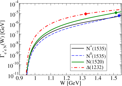
Figure 16: Comparison between Dalitz decay widths $\Gamma_{e^{+}e^{-}N}(W)$ for different resonances. Models from Refs. Timelike2 ; N1520TL . The diamonds indicate the Dalitz decay widths at the physical point ($W=M_{R}$).

Appendix A $\gamma^{\ast}N\to N(\frac{1}{2}^{-})$ form factors and helicity amplitudes

We discuss here the generic expressions for the form factors in different representations and their relations with the helicity amplitudes. The discussion follows Refs. Devenish76 ; Krivoruchenko02 , but is based on the current (1), where the form factors $F_{i}^{\ast}$ ($i=1,2$) are dimensionless. To compare with the results from Ref. Devenish76 one uses $G_{1}=q^{2}F_{1}^{\ast}$ and $G_{2}=\frac{2}{(M_{R}+M_{N})^{2}}F_{2}^{\ast}$.

The expressions associated with the decay widths can be expressed directly in terms of the helicity amplitudes, as in Eq. (44), or in terms of multipole form factors. Those form factors can be defined using different conventions as the ones proposed in Refs. Devenish76 ; Krivoruchenko02 . We use here a representation equivalent to those authors, but with different normalizations. More specifically, we use the following representation of the electric and Coulomb form factors:

$$G_{E} = F_{1}^{\ast}+\eta F_{2}^{\ast},$$ (45)

$$G_{C} = -\frac{M_{R}}{2}\frac{(M_{R}+M_{N})}{Q^{2}}\left[\eta F_{1}^{\ast}-\tau F_{2}^{\ast}\right].$$ (46)

The conversion to the form factors from Ref. Krivoruchenko02 , $\bar{G}_{E}$ and $\bar{G}_{C}$ can be performed using $\bar{G}_{E}=-\frac{\sqrt{2}}{M_{R}}G_{E}$ and $\bar{G}_{C}=-\frac{\sqrt{2}}{M_{R}}G_{C}$. To compare with the form factors from Ref. Devenish76 we can use $h_{1}=-\frac{2}{M_{R}}G_{C}$ and $h_{3}=-\frac{2}{M_{R}}G_{E}$. An advantage in the use of the form factors (45)–(46) is that they are dimensionless.

The motivation to the identification with the electric and Coulomb form factors are the result of the resemblance with the nucleon Sachs form factors $G_{C}\propto F_{1}-\frac{Q^{2}}{4M_{N}^{2}}F_{2}$ and $G_{M}\propto F_{1}+F_{2}$, combined with the connection between negative parity and positive parity multipole amplitudes. Recall that in the change from positive parity and negative parity states we should replace $G_{E}\leftrightarrow G_{M}$ Aznauryan12a ; Devenish76 ; Krivoruchenko02 .

The multipole form factors can be related to the helicity amplitudes (5)–(6) by

$$G_{E}=\frac{1}{\cal B}A_{1/2},$$ (47)

$$G_{C}=\frac{1}{\sqrt{2}{\cal B}}\frac{M_{R}}{|{\bf q}|}S_{1/2},$$ (48)

where

$${\cal B}=\frac{e}{2}\sqrt{\frac{Q_{+}^{2}}{M_{N}M_{R}K}}.$$ (49)

A simple consequence of the relations (47)–(48) is that, according to Siegert’s theorem, near the pseudothreshold, one has Siegert1 : $S_{1/2}\simeq\frac{1}{\sqrt{2}}\frac{|{\bf q}|}{M_{R}-M_{N}}A_{1/2}$, which imply that

$$G_{C}=2\frac{M_{R}-M_{N}}{M_{R}}G_{E},$$ (50)

when $Q^{2}=-(M_{R}-M_{N})^{2}$.

Another important remark is that Eq. (50) is valid also for complex form factors, $G_{E}$ and $G_{C}$. One has then a constraint for the real part and another for the imaginary part.

Appendix B Estimate of $G_{C}(0)$

In the present appendix we calculate the value of $G_{C}$ at $Q^{2}=0$ for proton target, based on the valence quark and meson cloud parametrization for the $F_{1}^{\ast}$ and $F_{2}^{\ast}$ form factors.

Starting from the definition (8) we can write

$$G_{C}=-\frac{1}{2}M_{R}(M_{R}-M_{N})\frac{F_{1}^{\ast}}{Q^{2}}+\frac{M_{R}}{2(M_{R}+M_{N})}F_{2}^{\ast}.$$ (51)

We can then consider the limit $Q^{2}=0$:

$$G_{C}(0) = -\frac{1}{2}M_{R}(M_{R}-M_{N})\left.\frac{F_{1}^{\ast}}{Q^{2}}\right|_{Q^{2}=0}$$ (52)

$$+\frac{M_{R}}{2(M_{R}+M_{N})}F_{2}^{\ast}(0).$$

The value of $F_{2}^{\ast}(0)$ is determined exclusively by the meson cloud contribution $F_{2}^{\rm mc}(0)=A(0)+B(0)$ according with Eq. (26). Recall that $A(0)$ and $B(0)$ are determined by by the fit to the data.

We focus now on the calculation of $\frac{F_{1}^{\ast}}{Q^{2}}$ in the limit $Q^{2}=0$. We recall that $F_{1}^{\ast}$ can be decomposed in two components ($F_{1}^{\rm B}+F_{1}^{\rm mc}$), and that both components scale with $Q^{2}$ near the photon point. Based on our parametrizations of the bare and meson cloud components, we can write:

$$\left.\frac{F_{1}^{\rm B}}{Q^{2}}\right|_{Q^{2}=0}=\frac{1}{3}\left.\frac{{\cal I}_{R}^{\prime}}{Q^{2}}\right|_{Q^{2}=0},$$ (53)

$$\left.\frac{F_{1}^{\rm mc}}{Q^{2}}\right|_{Q^{2}=0}=-\frac{C_{0}}{\Lambda_{C}^{2}},$$ (54)

using the notation of Eq. (36). In the first equation, we used also the result $\left.(3j_{1}^{S}+j_{1}^{A})\right|_{Q^{2}=0}=\frac{2}{3}$.

The factor $\left.{\cal I}_{R}^{\prime}\right|_{Q^{2}=0}$ can be calculated based on the definition

$${\cal I}_{R}^{\prime} = {\cal I}_{R}\sqrt{\frac{Q^{2}}{m_{\rho}^{2}+Q^{2}}}$$ (55)

$$= \frac{G_{D}(Q^{2})Q^{2}}{M_{N}(M_{R}+M_{N})}\sqrt{\frac{(M_{R}+M_{N})^{2}+Q^{2}}{m_{\rho}^{2}+Q^{2}}},$$

using the dipole approximation for ${\cal I}_{R}/|{\bf q}|$, according with Eq. (35). From this previous relation, we conclude that ${\cal I}_{R}^{\prime}/Q^{2}\to G_{D}(0)/(M_{N}m_{\rho})$ in the limit $Q^{2}=0$. As a consequence:

$$\left.\frac{F_{1}^{\rm B}}{Q^{2}}\right|_{Q^{2}=0}=\frac{1}{3}\frac{G_{D}(0)}{M_{N}m_{\rho}}.$$ (56)

Combined the previous results, we obtain

$$G_{C}(0) = \frac{1}{2}\frac{M_{R}}{M_{R}+M_{N}}F_{2}^{\ast}(0)+\frac{1}{2}M_{R}(M_{R}-M_{N})\frac{C_{0}}{\Lambda_{C}^{2}}$$ (57)

$$-\frac{1}{6}M_{R}(M_{R}-M_{N})\frac{G_{D}(0)}{M_{N}m_{\rho}}.$$

The corollary of this analysis is that the use of a small regulator (mass $m_{\rho}$) tends to reduce the magnitude of $G_{C}(0)$ (enhancement of the last term, more significant cancellation of terms). In alternative, the use of a large value for $m_{\rho}$ tend to increase the value of $G_{C}(0)$ (less significant cancellation of terms).

Appendix C Analytic extension of the overlap integrals to the timelike region

In the present appendix, we describe how we estimate the overlap integral ${\cal I}_{R}$ and the function ${\cal I}_{R}^{\prime}$ in the timelike region ($Q^{2}<0$). For the purpose of the discussion we recall that in general ${\cal I_{R}}$ is proportional to $|{\bf q}|$, and that in the semirelativistic approximation $|{\bf q}|\equiv|{\bf q}|_{\rm sr}=Q\sqrt{1+\tau}$. The effect of the factor $Z$ is discussed later.

Since, in the context of the semirelativistic approximation, we cannot extrapolate the overlap integral for $|{\bf q}|_{\rm sr}<0$, because the radial wave functions cannot be defined below $Q^{2}=0$, we use an analytic continuation of the overlap integral ${\cal I}_{R}$ defined in the spacelike region.

Our analytic continuation of ${\cal I}_{R}$ is based on the observation that ${\cal I}_{R}/|{\bf q}|$ is finite in the limit $Q^{2}=0$, and in the realization that ${\cal I}_{R}/|{\bf q}|$ can for small $Q^{2}$ be approximated by a dipole form:

$$\frac{{\cal I}_{R}^{\rm sr}}{|{\bf q}|_{\rm sr}}\simeq\frac{G_{D}(q^{2})}{M_{N}}=\frac{{\cal C}}{M_{N}}\left(\frac{\Lambda_{D}^{2}}{\Lambda_{D}^{2}-q^{2}}\right)^{2},$$ (58)

where ${\cal C}$ is a constant with no dimensions and $\Lambda_{D}$ a cutoff parameter. The upper index on ${\cal I}_{R}$ indicate the result of the integral in the semirelativistic approximation.

Our analytic extension is then based on the replacement

$$\frac{{\cal I}_{R}}{|{\bf q}|}\to\frac{G_{D}(q^{2})}{M_{N}}$$ (59)

in the $Q^{2}<0$ region. In simple words, we replace the numeric result $\frac{{\cal I}_{R}^{\rm sr}}{|{\bf q}|_{\rm sr}}$ from spacelike by a simple expression for $\frac{{\cal I}_{R}}{|{\bf q}|}$ for $Q^{2}<0$. We consider then an analytic continuation of the results for $Q^{2}>0$.

The consequence of this extension is that we estimate ${\cal I}_{R}$, using the relation (58):

$${\cal I}_{R}=G_{D}(q^{2})\frac{|{\bf q}|}{M_{N}},$$ (60)

where $|{\bf q}|$ represent the magnitude of the transition momentum in the general case [see Eq. (3)]. With this simple procedure, we obtain an analytic continuation of the function ${\cal I}_{R}/|{\bf q}|$ in the region $0\leq q^{2}\leq(M_{R}-M_{N})^{2}$. The transition form factors are then defined by continuity in the timelike region.

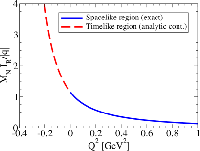
Figure 17: Representation of the function ${\cal I}_{R}/|{\bf q}|$ in terms of $Q^{2}$ in the spacelike and in the timelike regions, normalized by the factor $M_{N}$ (nucleon mass), for the case $W=1.535$ GeV. The results in spacelike region are determined by the quark model (SR approach). The results in the timelike region are determined by the analytic continuation based on the dipole form $G_{D}={\cal C}/(1+Q^{2}/\Lambda_{D}^{2})^{2}$, with the parameters ${\cal C}=1.154$ and $\Lambda_{D}^{2}=0.4396$ GeV².

Since the dipole approximation (58) generate necessarily singularities in the timelike region at $q^{2}=\Lambda_{D}^{2}$, it is necessary to regularize the expression including some effective width $\Gamma_{D}$, according to the replacement $\Lambda_{D}^{2}\to\Lambda_{D}^{2}-i\Lambda_{D}\Gamma_{D}$. For simplicity, we approximate the dipole function $G_{D}$, by the magnitude of $G_{D}$:

$$G_{D}(q^{2})\to{\cal C}\frac{\Lambda_{D}^{4}}{(\Lambda_{D}^{2}-q^{2})+\Lambda_{D}^{2}\Gamma_{D}^{2}}.$$ (61)

The explicit form of the function $\Gamma_{D}(q^{2})$ is discussed in the next subsection.

Combining the expression of ${\cal I}_{R}$ in the semirelativistic approximation, based on Eq. (58): ${\cal I}_{R}=G_{D}Q\sqrt{1+\tau}/M_{N}$, with $Z=Q/\sqrt{m_{\rho}^{2}+Q^{2}}$, we obtain

$${\cal I}_{R}^{\prime}\to\frac{G_{D}Q^{2}}{M_{N}(M_{R}+M_{N})}\sqrt{\frac{Q_{+}^{2}}{m_{\rho}^{2}+Q^{2}}}.$$ (62)

This expression is consistent with the results from spacelike, and ensures then the continuity between spacelike and timelike regions, provided that the normalization of $G_{D}$ is correct.

Note, however, that the relation (62) include a singularity for $q^{2}=m_{\rho}^{2}$. Since in the present study, our applications are restricted to the region $M_{R}<M_{N}+m_{\rho}$, we do not need to deal with the singularity $q^{2}=m_{\rho}^{2}$ directly. Nevertheless, we recall that the singularity $q^{2}=m_{\rho}^{2}$ is already present in the quark current (VMD parametrization). For consistence we regularize also the factor $1/\sqrt{m_{\rho}^{2}-q^{2}}$, as the remaining multipoles, according to Eq. (37), using $n=\frac{1}{2}$.

Explicit form for $\Gamma_{D}(q^{2})$

For the effective width $\Gamma_{D}$, we follow the regularization of previous works Timelike2 and use the form

$$\Gamma_{D}(q^{2})=\Gamma_{D}^{0}\left(\frac{q^{2}}{\Lambda_{D}^{2}+q^{2}}\right)^{2}\theta(q^{2}),$$ (63)

where $\theta$ is the Heaviside step function. The parameter $\Gamma_{D}^{0}$ define the range of influence of the regularization pole $q^{2}=\Lambda_{D}^{2}$. For very large values of $\Lambda_{D}$ we do not need to worry about the regularization and we can use the dipole form with $\Gamma_{D}=0$. However, for values of $\Lambda_{D}$ such that: $\Lambda_{D}\approx m_{\rho}$, as in the present case, the results can depend critically of the magnitude of $\Gamma_{D}^{0}$.

In order to obtain a timelike extension closer to the natural extension of the transition form factors (when $\Gamma_{D}^{0}=0$), and because the form factors are dominated by the imaginary part of the vector meson poles ($\rho$ and $\omega$) near $q^{2}=(W-M_{N})^{2}$, we choose $\Gamma_{D}^{0}=n\Gamma_{\rho}^{0}$, where $\Gamma_{\rho}^{0}$ is the $\rho$-meson physical width, and $n=1,2,...$ Larger values of $n$ lead to a significant reduction of the transition form factors, comparatively to an extension with $\Gamma_{D}^{0}=0$, near the pseudothreshold. Small values of $n$ ($n=1,2$) modify the transition form factors only slightly, except near the pseudothreshold. Comparing the final results for the Dalitz decay width, after the integration on $q$, we conclude that the results with $n=1,2,3,4$ are almost indistinguishable, showing that the results are almost independent of the regulator $\Gamma_{D}^{0}$.

In these conditions, we use $\Gamma_{D}^{0}=2\Gamma_{\rho}^{0}$. One obtains then transition form factors that are not very large near the pseudothreshold (as in the cases $n=0$ and $n=1$), generating smother functions for the Dalitz decay rates. As for the Dalitz decay widths, the results are almost insensitive to the value of $\Gamma_{D}^{0}$.

Appendix D Regularization of multipoles in the timelike region

To regularize the multipole factors associated with a effective cutoff (regulator) $\Lambda$, based on Eq. (37) we follow the procedure from Ref. N1520TL , and include the effective width

$$\Gamma_{\Lambda}(q^{2})=4\Gamma_{\Lambda}^{0}\left(\frac{q^{2}}{\Lambda^{2}+q^{2}}\right)^{2}\theta(q^{2}),$$ (64)

where $\theta$ is the Heaviside step function, and $\Gamma_{\Lambda}^{0}$ is a constant given by $\Gamma_{\Lambda}^{0}=4\Gamma_{\rho}^{0}\simeq 0.6$ GeV ($\Gamma_{\rho}^{0}$ is the $\rho$ physical decay constant).

The previous definition ensures that $\Gamma_{\Lambda}(q^{2})=0$ when $q^{2}<0$ and that $\Gamma_{\Lambda}(q^{2})$ is continuously extended for $q^{2}>0$. As a consequence, the results in the spacelike region (where there are no singularities) are kept unchanged. The factor $4\Gamma_{\Lambda}^{0}$ was chosen in order to obtain $\Gamma_{\Lambda}(q^{2})=\Gamma_{\Lambda}^{0}$ for $q^{2}=\Lambda^{2}$ and $\Gamma_{\Lambda}(q^{2})=4\Gamma_{\Lambda}^{0}$ for very large $q^{2}$. Finally, the value of $\Gamma_{\Lambda}^{0}$ was chosen to avoid very narrow peaks around $q^{2}=\Lambda^{2}$.

References

- (1) J. Adamczewski-Musch et al. [HADES Collaboration], Phys. Rev. C 95, 065205 (2017) [arXiv:1703.07840 [nucl-ex]].
- (2) W. J. Briscoe, M. Döring, H. Haberzettl, D. M. Manley, M. Naruki, I. I. Strakovsky and E. S. Swanson, Eur. Phys. J. A 51, 129 (2015) [arXiv:1503.07763 [hep-ph]].
- (3) G. Ramalho, M. T. Peña, J. Weil, H. van Hees and U. Mosel, Phys. Rev. D 93, 033004 (2016) [arXiv:1512.03764 [hep-ph]].
- (4) G. Ramalho and M. T. Peña, Phys. Rev. D 85, 113014 (2012) [arXiv:1205.2575 [hep-ph]];
- (5) G. Ramalho and M. T. Peña, Phys. Rev. D 95, 014003 (2017) [arXiv:1610.08788 [nucl-th]].
- (6) P. Cole, B. Ramstein and A. Sarantsev, Few Body Syst. 59, 144 (2018).
- (7) B. Ramstein et al. [HADES Collaboration], EPJ Web Conf. 199, 01008 (2019); B. Ramstein, Few Body Syst. 59, 143 (2018).
- (8) J. Weil, H. van Hees, and U. Mosel, Eur. Phys. J. A 48, 111 (2012) [Erratum-ibid. A 48, 150 (2012)] [arXiv:1203.3557 [nucl-th]].
- (9) E. L. Bratkovskaya, W. Cassing, M. Effenberger and U. Mosel, Nucl. Phys. A 653, 301 (1999) [nucl-th/9903009].
- (10) A. Faessler, C. Fuchs, M. I. Krivoruchenko and B. V. Martemyanov, J. Phys. G 29, 603 (2003) [nucl-th/0010056].
- (11) I. G. Aznauryan, A. Bashir, V. Braun, S. J. Brodsky, V. D. Burkert, L. Chang, C. Chen and B. El-Bennich et al., Int. J. Mod. Phys. E, 22, 1330015 (2013) [arXiv:1212.4891 [nucl-th]].
- (12) B. Ramstein [HADES Collaboration], Few Body Syst. 59, 141 (2018).
- (13) J. Adamczewski-Musch et al. [HADES Collaboration], Eur. Phys. J. A 53, 149 (2017) [arXiv:1703.08575 [nucl-ex]].
- (14) G. Agakishiev et al., Eur. Phys. J. A 50, 82 (2014) [arXiv:1403.3054 [nucl-ex]]; G. Agakishiev et al. [HADES Collaboration], Phys. Rev. C 85, 054005 (2012) [arXiv:1203.2549 [nucl-ex]]; G. Agakishiev et al. [HADES Collaboration], Phys. Lett. B 715, 304 (2012) [arXiv:1205.1918 [nucl-ex]]; G. Agakishiev et al. [HADES Collaboration], Eur. Phys. J. A 48, 64 (2012) [arXiv:1112.3607 [nucl-ex]].
- (15) G. Agakishiev et al. [HADES Collaboration], Eur. Phys. J. A 51, 137 (2015); G. Agakishiev et al. [HADES Collaboration], Eur. Phys. J. A 48, 74 (2012) [arXiv:1203.1333 [nucl-ex]]; G. Agakishiev et al. [HADES Collaboration], Phys. Lett. B 690, 118 (2010) [arXiv:0910.5875 [nucl-ex]].
- (16) G. Ramalho and M. T. Peña, Phys. Rev. D 84, 033007 (2011) [arXiv:1105.2223 [hep-ph]].
- (17) G. Ramalho and K. Tsushima, Phys. Rev. D 84, 051301 (2011) [arXiv:1105.2484 [hep-ph]].
- (18) G. Ramalho, D. Jido and K. Tsushima, Phys. Rev. D 85, 093014 (2012) [arXiv:1202.2299 [hep-ph]].
- (19) B. Julia-Diaz, H. Kamano, T.-S. H. Lee, A. Matsuyama, T. Sato and N. Suzuki, Phys. Rev. C 80, 025207 (2009) [arXiv:0904.1918 [nucl-th]].
- (20) D. Jido, M. Döring and E. Oset, Phys. Rev. C 77, 065207 (2008).
- (21) I. G. Aznauryan and V. Burkert, Phys. Rev. C 95, 065207 (2017) [arXiv:1703.01751 [nucl-th]].
- (22) V. M. Braun et al., Phys. Rev. Lett. 103, 072001 (2009) [arXiv:0902.3087 [hep-ph]].
- (23) I. V. Anikin, V. M. Braun and N. Offen, Phys. Rev. D 92, 014018 (2015) [arXiv:1505.05759 [hep-ph]].
- (24) V. D. Burkert and T. S. H. Lee, Int. J. Mod. Phys. E 13, 1035 (2004) [nucl-ex/0407020].
- (25) H. Kamano, S. X. Nakamura, T. S. H. Lee and T. Sato, Phys. Rev. C 94, 015201 (2016) [arXiv:1605.00363 [nucl-th]].
- (26) Z. W. Liu, W. Kamleh, D. B. Leinweber, F. M. Stokes, A. W. Thomas and J. J. Wu, Phys. Rev. Lett. 116, 082004 (2016) [arXiv:1512.00140 [hep-lat]].
- (27) T. Gutsche, V. E. Lyubovitskij and I. Schmidt, Phys. Rev. D 101, 034026 (2020) [arXiv:1911.00076 [hep-ph]].
- (28) A. Ballon-Bayona, H. Boschi-Filho, N. R. F. Braga, M. Ihl and M. A. C. Torres, Phys. Rev. D 86, 126002 (2012) [arXiv:1209.6020 [hep-ph]].
- (29) I. T. Obukhovsky, A. Faessler, D. K. Fedorov, T. Gutsche and V. E. Lyubovitskij, Phys. Rev. D 100, 094013 (2019) [arXiv:1909.13787 [hep-ph]].
- (30) F. Gross, G. Ramalho and M. T. Peña, Phys. Rev. C 77, 015202 (2008) [nucl-th/0606029].
- (31) G. Ramalho, K. Tsushima and F. Gross, Phys. Rev. D 80, 033004 (2009) [arXiv:0907.1060 [hep-ph]].
- (32) G. Ramalho, Few Body Syst. 59, 92 (2018) [arXiv:1801.01476 [hep-ph]].
- (33) G. Ramalho, Phys. Rev. D 95, 054008 (2017) [arXiv:1612.09555 [hep-ph]].
- (34) G. Ramalho and M. T. Peña, Phys. Rev. D 89, 094016 (2014) [arXiv:1309.0730 [hep-ph]].
- (35) G. Ramalho, Phys. Rev. D 90, 033010 (2014) [arXiv:1407.0649 [hep-ph]].
- (36) G. Ramalho, M. T. Peña and F. Gross, Eur. Phys. J. A 36, 329 (2008) [arXiv:0803.3034 [hep-ph]]; G. Ramalho, M. T. Peña and F. Gross, Phys. Rev. D 78, 114017 (2008) [arXiv:0810.4126 [hep-ph]].
- (37) G. Ramalho and K. Tsushima, Phys. Rev. D 81 (2010) 074020 [arXiv:1002.3386 [hep-ph]]; G. Ramalho and K. Tsushima, Phys. Rev. D 89, 073010 (2014) [arXiv:1402.3234 [hep-ph]].
- (38) G. Ramalho and K. Tsushima, Phys. Rev. D 82, 073007 (2010) [arXiv:1008.3822 [hep-ph]].
- (39) E. E. Jenkins and A. V. Manohar, Phys. Lett. B 255, 558 (1991).
- (40) I. G. Aznauryan and V. D. Burkert, Prog. Part. Nucl. Phys. 67, 1 (2012) [arXiv:1109.1720 [hep-ph]].
- (41) G. Eichmann and G. Ramalho, Phys. Rev. D 98, 093007 (2018) [arXiv:1806.04579 [hep-ph]].
- (42) G. Ramalho, Phys. Lett. B 759, 126 (2016) [arXiv:1602.03444 [hep-ph]].
- (43) R. C. E. Devenish, T. S. Eisenschitz and J. G. Korner, Phys. Rev. D 14, 3063 (1976).
- (44) G. Ramalho, Phys. Rev. D 100, 114014 (2019) [arXiv:1909.00013 [hep-ph]].
- (45) Comparative to Refs. N1535 ; Aznauryan12a the form factors are modified by a sign, according with the choice in Ref. Aznauryan12a .
- (46) M. I. Krivoruchenko, B. V. Martemyanov, A. Faessler and C. Fuchs, Annals Phys. 296, 299 (2002) [nucl-th/0110066].
- (47) I. G. Aznauryan et al. [CLAS Collaboration], Phys. Rev. C 80, 055203 (2009) [arXiv:0909.2349 [nucl-ex]].
- (48) M. M. Dalton et al., Phys. Rev. C 80, 015205 (2009) [arXiv:0804.3509 [hep-ex]].
- (49) D. Drechsel, S. S. Kamalov and L. Tiator, Eur. Phys. J. A 34, 69 (2007) [arXiv:0710.0306 [nucl-th]];
- (50) L. Tiator, D. Drechsel, S. S. Kamalov and M. Vanderhaeghen, Chin. Phys. C 33, 1069 (2009) [arXiv:0909.2335 [nucl-th]].
- (51) M. Tanabashi et al. [Particle Data Group], Phys. Rev. D 98, 030001 (2018).
- (52) F. Gross, Phys. Rev. 186, 1448 (1969); A. Stadler, F. Gross and M. Frank, Phys. Rev. C 56, 2396 (1997). [arXiv:nucl-th/9703043].
- (53) F. Gross, G. Ramalho and M. T. Peña, Phys. Rev. D 85, 093005 (2012) [arXiv:1201.6336 [hep-ph]].
- (54) G. Ramalho, K. Tsushima and A. W. Thomas, J. Phys. G 40, 015102 (2013) [arXiv:1206.2207 [hep-ph]]; G. Ramalho, J. P. B. C. de Melo and K. Tsushima, Phys. Rev. D 100, 014030 (2019) [arXiv:1902.08844 [hep-ph]].
- (55) F. Gross, G. Ramalho and M. T. Peña, Phys. Rev. D 85, 093006 (2012) [arXiv:1201.6337 [hep-ph]].
- (56) G. Ramalho and K. Tsushima, Phys. Rev. D 94, 014001 (2016) [arXiv:1512.01167 [hep-ph]].
- (57) G. Ramalho, M. T. Peña and F. Gross, Phys. Rev. D 81, 113011 (2010) [arXiv:1002.4170 [hep-ph]]; G. Ramalho and M. T. Peña, J. Phys. G 36, 085004 (2009) [arXiv:0807.2922 [hep-ph]].
- (58) G. Ramalho and M. T. Peña, Phys. Rev. D 80 (2009) 013008 [arXiv:0901.4310 [hep-ph]].
- (59) G. Ramalho and M. T. Peña, J. Phys. G 36, 115011 (2009) [arXiv:0812.0187 [hep-ph]].
- (60) F. Gross, G. Ramalho and K. Tsushima, Phys. Lett. B 690, 183 (2010) [arXiv:0910.2171 [hep-ph]]; G. Ramalho and K. Tsushima, Phys. Rev. D 84, 054014 (2011) [arXiv:1107.1791 [hep-ph]].
- (61) G. Ramalho and K. Tsushima, Phys. Rev. D 87, 093011 (2013) [arXiv:1302.6889 [hep-ph]].
- (62) arXiv:2002.07280 [hep-ph].
- (63) G. Ramalho, M. T. Peña and K. Tsushima, Phys. Rev. D 101, 014014 (2020) [arXiv:1908.04864 [hep-ph]].
- (64) J. J. Kelly, Phys. Rev. C 56, 2672 (1997).
- (65) Z. Batiz and F. Gross, Phys. Rev. C 58, 2963 (1998) [arXiv:nucl-th/9803053].
- (66) R. A. Gilman and F. Gross, J. Phys. G 28, R37 (2002) [nucl-th/0111015].
- (67) C. E. Carlson and N. C. Mukhopadhyay, Phys. Rev. Lett. 81, 2646 (1998) [hep-ph/9804356]; C. E. Carlson, Few Body Syst. Suppl. 11, 10 (1999) [hep-ph/9809595].
- (68) F. Iachello, A. D. Jackson and A. Lande, Phys. Lett. B 43, 191 (1973).
- (69) F. Iachello and Q. Wan, Phys. Rev. C 69, 055204 (2004); R. Bijker and F. Iachello, Phys. Rev. C 69, 068201 (2004) [arXiv:nucl-th/0405028].
- (70) F. Dohrmann et al., Eur. Phys. J. A 45, 401 (2010) [arXiv:0909.5373 [nucl-ex]].
- (71) Check chapter 97 from Ref. PDG .