Drawing Graphs
with Circular Arcs and Right-Angle Crossings

Abstract

In a RAC drawing of a graph, vertices are represented by points in the plane, adjacent vertices are connected by line segments, and crossings must form right angles. Graphs that admit such drawings are RAC graphs. RAC graphs are beyond-planar graphs and have been studied extensively. In particular, it is known that a RAC graph with $n$ vertices has at most $4n-10$ edges.

We introduce a superclass of RAC graphs, which we call arc-RAC graphs. A graph is arc-RAC if it admits a drawing where edges are represented by circular arcs and crossings form right angles. We provide a Turán-type result showing that an arc-RAC graph with $n$ vertices has at most $14n-12$ edges and that there are $n$-vertex arc-RAC graphs with $4.5n-O(\sqrt{n})$ edges.

1 Introduction

A drawing of a graph in the plane is a mapping of its vertices to distinct points and each edge $uv$ to a curve whose endpoints are $u$ and $v$. Planar graphs, which admit crossing-free drawings, have been studied extensively. They have many nice properties and several algorithms for drawing them are known, see, e.g., [20, 21]. However, in practice we must also draw non-planar graphs and crossings make it difficult to understand a drawing. For this reason, graph classes with restrictions on crossings are studied, e.g., graphs that can be drawn with at most $k$ crossings per edge (known as $k$-planar graphs) or where the angles formed by each crossing are “large”. These classes are categorized as beyond-planar graphs and have experienced increasing interest in recent years [14].

As introduced by Didimo et al. [13], a prominent beyond-planar graph class that concerns the crossing angles is the class of $k$-bend right-angle-crossing graphs, or RAC_k graphs for short, that admit a drawing where all crossings form $90^{\circ}$ angles and each edge is a polygonal chain with at most $k$ bends. Using right-angle crossings and few bends is motivated by several cognitive studies suggesting a positive correlation between large crossing angles or small curve complexity and the readability of a graph drawing [17, 18, 19]. Didimo et al. [13] studied the edge density of RAC_k graphs. They showed that RAC₀ graphs with $n$ vertices have at most $4n-10$ edges (which is tight), that RAC₁ graphs have at most $O(n^{\frac{4}{3}})$ edges, that RAC₂ graphs have at most $O(n^{\frac{7}{4}})$ edges and that all graphs are RAC₃. Dujmović et al. [15] gave an alternative simple proof of the $4n-10$ bound for RAC₀ graphs using charging arguments similar to those of Ackerman and Tardos [2] and Ackerman [1]. Arikushi et al. [6] improved the upper bounds to $6.5n-13$ for RAC₁ graphs and to $74.2n$ for RAC₂ graphs. The bound of $6.5n-13$ for RAC₁ graphs was also obtained by charging arguments. They also provided a RAC₁ graph with $4.5n-O(\sqrt{n})$ edges. The best known lower and upper bound for the maximum edge density of RAC₁ graphs of $5n-10$ and $5.5n-11$, respectively, are due to Angelini et al. [4].

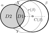
We extend the class of RAC₀ graphs by allowing edges to be drawn as circular arcs but still requiring $90^{\circ}$ crossings. An angle at which two circles intersect is the angle between the two tangents to each of the circles at an intersection point. Two circles intersecting at a right angle are called orthogonal. For any circle $\gamma$, let $C({\gamma})$ be its center and let $r({\gamma})$ be its radius. The following observation follows from the Pythagorean theorem.

Figure 1: Circles $\alpha$ and $\beta$ are orthogonal if and only if $\triangle XC({\alpha})C({\beta})$ is right-angled.

Observation .

Let $\alpha$ and $\beta$ be two circles. Then $\alpha$ and $\beta$ are orthogonal if and only if $r({\alpha})^{2}+r({\beta})^{2}=|C({\alpha})C({\beta})|^{2}$; see Figure 1.

In addition we note the following.

Observation .

Given a pair of orthogonal circles, the tangent to one circle at one of the intersection points goes through the center of the other circle; see Figure 1. In particular, a line is orthogonal to a circle if the line goes through the center of the circle.

Similarly, two circular arcs $\alpha$ and $\beta$ are orthogonal if they intersect properly (that is, ignoring intersections at endpoints) and the underlying circles (that contain the arcs) are orthogonal. For the remainder of this paper, all arcs will be circular arcs. We consider any straight-line segment to be an arc with infinite radius. Note, though, that the above observations do not hold for (pairs of) circles of infinite radius. As in the case of circles, for any arc $\gamma$ of finite radius, let $C({\gamma})$ be its center.

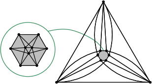
We call a drawing of a graph an arc-RAC drawing if the edges are drawn as arcs and any pair of intersecting arcs is orthogonal; see Figure 2. A graph that admits an arc-RAC drawings is called an arc-RAC graph.

Figure 2: An arc-RAC drawing of a graph. This graph is not RAC₀ [7].

The idea of drawing graphs with arcs dates back to at least the work of the artist Mark Lombardi who drew social networks, featuring players from the political and financial sector [23]. Indeed, user studies [26, 28] state that users prefer edges drawn with curves of small curvature; not necessarily for performance (that is, tasks such as finding shortest paths, identifying common neighbors, or determining vertex degrees) but for aesthetics. Drawing graphs with arcs can help to improve certain quality measures of a drawing such as angular resolution [12, 3] or visual complexity [27, 22].

An immediate restriction on the edge density of arc-RAC graphs is imposed by the following known result.

Lemma 1.1 ([24]).

In an arc-RAC drawing, there cannot be four pairwise orthogonal arcs.

It follows from Lemma 1.1 that arc-RAC graphs are $4$-quasi-planar, that is, an arc-RAC drawing cannot have four edges that pairwise cross. This implies that an arc-RAC graph with $n$ vertices can have at most $72(n-2)$ edges [1].

Our main contribution is that we reduce this bound to $14n-12$ using charging arguments similar to those of Ackerman [1] and Dujmović et al. [15]; see Section 2. For us, the main challenge was to apply these charging arguments to a modification of an arc-RAC drawing and to exploit, at the same time, geometric properties of the original arc-RAC drawing to derive the bound. We also provide a lower bound of $4.5n-O(\sqrt{n})$ on the maximum edge density of arc-RAC graphs based on the construction of Arikushi et al. [6]; see Section 3. We conclude with some open problems in Section 4. Throughout the paper our notation won’t distinguish between the entities (vertices and edges) of an abstract graph and the geometric objects (points and curves) representing them in a drawing.

As usual for topological drawings, we forbid vertices to lie in the relative interior of an edge and we do not allow edges to touch, that is, to have a common point in their relative interiors without crossing each other at this point. Hence an intersection point of two edges is always a crossing. When we say that two edges share a point, we mean that they either cross each other or have a common endpoint.

2 An Upper Bound for the Maximum Edge Density

Let $G$ be a $4$-quasi-planar graph, and let $D$ be a $4$-quasi-planar drawing of $G$. In his proof of the upper bound on the edge density of $4$-quasi-planar graphs, Ackerman [1] first modified the given drawing so as to remove faces of small degree. We use a similar modification that we now describe.

Consider two edges $e_{1}$ and $e_{2}$ in $D$ that intersect multiple times. A region in $D$ bounded by pieces of $e_{1}$ and $e_{2}$ that connect two consecutive crossings or a crossing and a vertex of $G$ is called a lens. If a lens is adjacent to a crossing and a vertex of $G$, then we call such a lens a 1-lens, otherwise a 0-lens. A lens that does not contain a vertex of $G$ is empty.

Figure 3: A simplification step resolves a smallest empty 0-lens; if two edges $e_{1}$ and $e_{2}$ change the order in which they cross the edge $e$, they form an empty 0-lens intersecting $e$ before the step, and thus, in the original $4$-quasi-planar drawing.

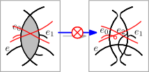
Every drawing with 0-lenses has a smallest empty 0-lens, that is, an empty 0-lens that does not contain any other empty 0-lenses in its interior. We can swap [25, 1] the two curves that bound a smallest empty 0-lens; see Figure 3. We call such a swap a simplification step. Since a simplification step resolves a smallest empty lens, we observe the following.

Observation 2.1.

A simplification step does not introduce any new pairs of crossing edges or any new empty lenses.

We exhaustively apply simplification steps to our drawing and refer to this as the simplification process. Observation 2.1 guarantees that applying the simplification process to a drawing $D$ terminates, that is, it results in an empty-0-lens-free drawing $D^{\prime}$ of $G$. We call the resulting drawing $D^{\prime}$ simplified; it is a simplification of $D$. Observation 2.1 implies the following important property of any simplification step.

Observation 2.2.

Applying a simplification step to a $4$-quasi-planar drawing yields a $4$-quasi-planar drawing.

As mentioned above, Ackerman [1] used a similar modification to prepare a $4$-quasi-planar drawing for his charging arguments; note, that unlike Ackerman, we do not resolve 1-lenses. We look at the simplification process in more detail, in particular, we consider how it changes the order in which edges cross.

Lemma 2.3.

Let $D$ be an arc-RAC drawing, and let $D^{\prime}$ be a simplification of $D$. If two edges $e_{1}$ and $e_{2}$ cross another edge $e$ in $D^{\prime}$ in an order different from that in $D$, then $e_{1}$ and $e_{2}$ form an empty 0-lens intersecting $e$ in $D$.

Proof 2.4.

Let $e_{1}$ and $e_{2}$ be two edges as in the statement of the lemma. Then there is a simplification step $i$ where the order in which $e_{1}$ and $e_{2}$ cross $e$ changes. Let $D_{i}$ be the drawing immediately before simplification step $i$, and let $D_{i+1}$ be the drawing right after step $i$. By construction, the order in which $e_{1}$ and $e_{2}$ cross $e$ is different in $D_{i}$ and in $D_{i+1}$. Since $D_{i}$ is $4$-quasi-planar (see Observation 2.2) and since we always resolve a smallest empty 0-lens, the edges $e_{1}$ and $e_{2}$ form a smallest empty 0-lens in $D_{i}$; see Figure 3. Given that the simplification process does not introduce new empty lenses (see Observation 2.1), $e_{1}$ and $e_{2}$ form an empty 0-lens in the original $4$-quasi-planar drawing.

We now focus on the special type of $4$-quasi-planar drawings we are interested in. Suppose that $G$ is an arc-RAC graph, $D$ is an arc-RAC drawing of $G$, and $D^{\prime}$ is a simplification of $D$. Note that, in general, $D^{\prime}$ is not an arc-RAC drawing. If two edges $e_{1}$ and $e_{2}$ cross in $D^{\prime}$, then they do not form an empty 0-lens in $D$. This holds because for any two edges forming an empty 0-lens in $D$, the simplification process removes both of their crossings; therefore, in $D^{\prime}$ the two edges do not have any crossings. If $e_{1}$ and $e_{2}$ are incident to the same vertex, they also do not form an empty 0-lens in $D$, as otherwise they would share three points in $D$ (the two crossing points of the lens and the common vertex of $G$). Thus, we have the following observation.

Observation 2.5.

Let $D$ be an arc-RAC drawing, and let $D^{\prime}$ be a simplification of $D$. If two edges $e_{1}$ and $e_{2}$ share a point in $D^{\prime}$, then they do not form an empty 0-lens in $D$.

In the following, we first state the main theorem of this section and provide the structure of its proof (deferring one small lemma and the main technical lemma until later). Then, we prove the remaining technical details in Lemmas 2.8 to 2.16 to establish the result.

Theorem 2.6.

An arc-RAC graph with $n$ vertices can have at most $14n-12$ edges.

Proof 2.7.

Let $G=(V,E)$ be an arc-RAC graph, let $D$ be an arc-RAC drawing of $G$, let $D^{\prime}$ be a simplification of $D$, and let $G^{\prime}=(V^{\prime},E^{\prime})$ be the planarization of $D^{\prime}$. Our charging argument consists of three steps.

First, each face $f$ of $G^{\prime}$ is assigned an initial charge $ch({f})=|f|+v(f)-4$, where $|f|$ is the degree of $f$ in the planarization and $v(f)$ is the number of vertices of $G$ on the boundary of $f$. Applying Euler’s formula several times, Ackerman and Tardos [2] showed that $\sum_{f\in G^{\prime}}ch({f})=4n-8$, where $n$ is the number of vertices of $G$. In addition, we set the charge $ch({v})$ of a vertex $v$ of $G$ to $16/3$. Hence the total charge of the system is $4n-8+16n/3=28n/3-8$.

In the next two steps (described below), similarly to Dujmović et al. [15], we redistribute the charges among faces of $G^{\prime}$ and vertices of $G$ so that, for every face $f$, the final charge $ch_{\mathrm{fin}}({f})$ is at least $v(f)/3$ and the final charge of each vertex is non-negative. Observing that

$$28n/3-8\geq\sum_{f\in G^{\prime}}ch_{\mathrm{fin}}({f})\geq\sum_{f\in G^{\prime}}v(f)/3=\sum_{v\in G}\deg(v)/3=2|E|/3$$

yields that the number of edges of $G$ is at most $14n-12$ as claimed. (The second-last equality holds since both sides count the number of vertex–face incidences in $G^{\prime}$.)

After the first charging step above, it is easy to see that $ch({f})\geq v(f)/3$ holds if $|f|\geq 4$. We call a face $f$ of $G^{\prime}$ a $k$-triangle, $k$-quadrilateral, or $k$-pentagon if $f$ has the corresponding shape and $v(f)=k$. Similarly, we call a face of degree two a digon. Note that any digon is a 1-digon since all empty 0-lenses have been simplified.

After the first charging step, each digon and each 0-triangle has a charge of $-1$, and each 1-triangle has a charge of $0$. Thus, in the second charging step, we need to find ${4}/{3}$ units of charge for each digon, one unit of charge for each 0-triangle, and ${1}/{3}$ unit of charge for each 1-triangle. Note that all other faces including 2- and 3-triangles already have sufficient charge.

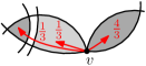
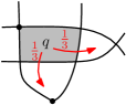
To charge a digon $d$ incident to a vertex $v$ of $G$, we decrease $ch({v})$ by $4/3$ and increase $ch({d})$ by $4/3$; see Figure 4(a). We say that $v$ contributes charge to $d$.

To charge triangles, we proceed similarly to Ackerman [1] and Dujmović et al. [15, Theorem 7].

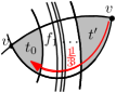
Consider a $1$-triangle $t_{1}$. Let $v$ be the unique vertex incident to $t_{1}$, and let $s_{1}\in E^{\prime}$ be the edge of $t_{1}$ opposite of $v$; see Figure 4(b). Note that the endpoints of $s_{1}$ are intersection points in $D^{\prime}$. Let $f_{1}$ be the face on the other side of $s_{1}$. If $f_{1}$ is a $0$-quadrilateral, then we consider its edge $s_{2}\in E^{\prime}$ opposite to $s_{1}$ and the face $f_{2}$ on the other side of $s_{2}$. We continue iteratively until we meet a face $f_{k}$ that is not a $0$-quadrilateral. If $f_{k}$ is a triangle, then all the faces $t_{1},f_{1},f_{2},\dots,f_{k}$ belong to the same empty 1-lens $l$ incident to the vertex $v$ of $t_{1}$. In this case, we decrease $ch({v})$ by $1/3$ and increase $ch({t_{1}})$ by $1/3$; see Figure 4(a). Otherwise, $f_{k}$ is not a triangle and $|f_{k}|+v(f_{k})-4\geq 1$ (see Figure 4(b)). In this case, we decrease $ch({f_{k}})$ by $1/3$ and increase $ch({t_{1}})$ by $1/3$. We say that the face $f_{k}$ contributes charge to the triangle $t_{1}$ over its side $s_{k}$.

For a 0-triangle $t_{0}$, we repeat the above charging over each side. If the last face on our path is a triangle $t^{\prime}$, then $t_{0}$ and $t^{\prime}$ are contained in an empty 1-lens (recall that $D^{\prime}$ does not contain empty 0-lenses) and $t^{\prime}$ is a 1-triangle incident to a vertex $v$ of $G$. In this case, we decrease $ch({v})$ by $1/3$ and increase $ch({t_{0}})$ by $1/3$; see Figure 4(c).

Thus, at the end of the second step, the charge of each digon and triangle $f$ is at least $v(f)/3$. Note that the charge of $f$ comes either from a higher-degree face or from a vertex $v$ incident to an empty 1-lens containing $f$.

In the third step, we do not modify the charging any more, but we need to ensure that

1. $ch({f})\geq v(f)/3$ still holds for each face $f$ of $G^{\prime}$ with $|f|\geq 4$ and

2. $ch({v})\geq 0$ for each $v$ of $G$.

We first show statement (i). Ackerman [1] noted that a face $f$ with $|f|\geq 4$ can contribute charges over each of its edges at most once. Moreover, $f$ can contribute at most one third unit of charge over each of its edges. Therefore, if $|f|+v(f)\geq 6$, then in the worst case (that is, $f$ contributes charge over each of its edges) $f$ still has a charge of $|f|+v(f)-4-|f|/3\geq v(f)/3$. Thus, it remains to verify that 1-quadrilaterals and 0-pentagons, which initially had only one unit of charge, have a charge of at least $1/3$ unit or zero, respectively, at the end of the second step.

A 1-quadrilateral $q$ can contribute charge to at most two triangles since the endpoints of any edge of $G^{\prime}$ over which a face contributes charge must be intersection points in $D^{\prime}$; see Figure 4(d) and recall that $q$ now plays the role of $f_{k}$ in Figure 4(b).

A 0-pentagon cannot contribute charge to more than three triangles; see Lemma 2.16.

Now we show statement (ii). Recall that a vertex $v$ can contribute charge to a digon incident to $v$ or to at most two triangles contained in an empty 1-lens incident to $v$. Observe that two empty 1-lenses with either triangles or a digon taking charge from $v$ cannot overlap; see Figure 4(a). We show in Lemma 2.8 that $v$ cannot be incident to more than four such empty 1-lenses. In the worst case, $v$ contributes ${4}/{3}$ units of charge to each of the at most four incident digons representing these empty 1-lenses. Thus, $v$ has non-negative charge at the end of the second step.

(a) Vertex $v$ contributes charge to a digon and two triangles contained in empty 1-lenses.

(b) Face $f_{k}$ contributes charge to the 1-triangle $t_{1}$.

(c) Vertex $v$ contributes charge to the 0-triangle $t_{0}$.

(d) 1-quadrilateral $q$ contributes charge to at most two triangles.

Figure 4: Transferring charge from vertices and high-degree faces to small-degree faces.

Lemma 2.8.

In any simplified arc-RAC drawing, each vertex is incident to at most four non-overlapping empty 1-lenses.

Proof 2.9.

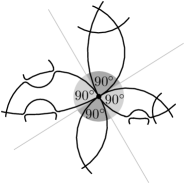
Let $v$ be a vertex incident to some non-overlapping empty 1-lenses. Consider a small neighborhood of the vertex $v$ in the simplified drawing and notice that in this neighborhood the simplified drawing is the same as the original arc-RAC drawing. Let $l$ be one of the non-overlapping empty 1-lenses incident to $v$. Then $l$ forms an angle of $90^{\circ}$ between the two edges incident to $v$ that form $l$; see Figure 6. This is due to the fact that the other “endpoint” of $l$ is an intersection point where the two edges must meet at $90^{\circ}$. Thus $v$ is incident to at most four non-overlapping empty 1-lenses.

Figure 5: The edges of an empty 1-lens form a $\pi/2$ angle at the vertex of the lens.

Figure 6: The relation $\Pi({\cdot\;};{\,\cdot})$ does not necessarily describe all intersection points along an edge. Here, e.g., $\Pi({e};{e_{1},e_{2},e_{3},e_{4},e_{3},e_{5},e_{6}})$ and $\Pi({e};{e_{1},e_{3},e_{4},e_{5}})$ both hold.

We now set the stage for proving Lemma 2.16, which shows that a 0-pentagon in a simplified drawing does not contribute charge to more than three triangles. The proof goes by a contradiction. Consider a 0-pentagon that contributes charge to at least four triangles in the simplified drawing. First, we examine which edges of this 0-pentagon cross; see Lemma 2.10. We then describe the order in which these edges share points in the simplified drawing and show that the original arc-RAC drawing must adhere to the same order; see Lemma 2.12. Finally, we use geometric arguments to show that, under these order constraints, an arc-RAC drawing of the edges does not exist; see Lemma 2.14.

Let $D$ be an arc-RAC drawing of some arc-RAC graph $G=(V,E)$, let $D^{\prime}$ be its simplification, and let $p$ be a 0-pentagon that contributes charge to at least four triangles. Let $s_{0},s_{1},\dots,s_{4}$ be the sides of $p$ in clockwise order and denote the edges of $G$ that contain these sides as $e_{0},e_{1},\dots,e_{4}$ so that edge $e_{0}$ contains side $s_{0}$ etc. Since $p$ contributes charge over at least four sides, these sides are consecutive around $p$. Without loss of generality, we assume that $s_{4}$ is the side over which $p$ does not necessarily contribute charge.

For $i\in\{0,1,2,3\}$, let $t_{i}$ be the triangle that gets charge from $p$ over the side $s_{i}$. The triangle $t_{i}$ is bounded by the edges $e_{i-1}$ and $e_{i+1}$. (Indices are taken modulo $5$.) Note that all faces bounded by $e_{i-1}$ and $e_{i+1}$ that are between $t_{i}$ and $p$ must be 0-quadrilaterals. If $t_{i}$ is a 1-triangle, then $e_{i-1}$ and $e_{i+1}$ are incident to the same vertex of the triangle. Otherwise, $t_{i}$ is a 0-triangle and $e_{i-1}$ and $e_{i+1}$ cross at a vertex of the triangle. Let $A^{\prime}_{i-1,i+1}$ denote this common point of $e_{i-1}$ and $e_{i+1}$, and let $E_{p}=\{e_{0},\dots,e_{4}\}$; see Figure 7(a).

(a) Notation: A 0-pentagon $p$ in $D^{\prime}$ and the edges in $E_{p}$. The points of type $A^{\prime}_{i-1,i+1}$ are either intersection points or vertices of $G$.

(b) Also in $D$, it holds that $\Pi({e_{0}};{e_{4},e_{1},e_{2}})$, $\Pi({e_{3}};{e_{1},e_{2},e_{4}})$, and, for $i\in\{1,2,4\}$, $\Pi({e_{i}};{e_{i-2},e_{i-1},e_{i+1},e_{i+2}})$.

Figure 7: A $0$-pentagon cannot contribute charge to more than three triangles.

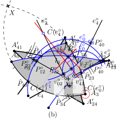
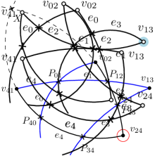
We now describe the order in which the edges in $E_{p}$ share points in $D^{\prime}$. To this end, we orient the edges in $E_{p}$ so that this orientation conforms with the orientation of a clockwise walk around the boundary of $p$ in $D^{\prime}$. In addition, we write $\Pi({e_{k}};{e_{i_{1}},e_{i_{2}},\dots,e_{i_{l}}})$ if the edge $e_{k}$ shares points (either crossing points or vertices of the graph) with the edges $e_{i_{1}},e_{i_{2}},\dots,e_{i_{l}}$ in this order with respect to the orientation of $e_{k}$; see Figure 6. (Note that we can have $\Pi({e_{k}};{e_{i},e_{j},e_{i}})$ as edges may intersect twice. We will not consider more than two edges sharing the same endpoint.) Due to the order in which we numbered the edges in $E_{p}$, it holds in $D^{\prime}$ that $\Pi({e_{0}};{e_{4},e_{1},e_{2}})$, $\Pi({e_{3}};{e_{1},e_{2},e_{4}})$, and, for $i\in\{1,2,4\}$, $\Pi({e_{i}};{e_{i-2},e_{i-1},e_{i+1},e_{i+2}})$; see Figure 7(a). Now we show that in $D$ the order is the same. Obviously every pair of edges $(e_{i-1},e_{i+1})$ that shares an endpoint in $D^{\prime}$ also shares an endpoint in $D$. Furthermore, every pair $(e_{i},e_{i+1})$ or $(e_{i-1},e_{i+1})$ of crossing edges crosses in $D$, too, because the simplification process does not introduce new pairs of crossing edges; see Observation 2.1.

Lemma 2.10.

In the drawing $D$, the edges $e_{0}$ and $e_{3}$ do not cross.

Proof 2.11.

Assume that the edges $e_{0}$ and $e_{3}$ cross in $D$ and notice that each of the pairs of edges $(e_{0},e_{1})$, $(e_{1},e_{2})$, and $(e_{2},e_{3})$ forms a crossing in $D^{\prime}$ (see Figure 7(a)), and hence in $D$, too. For any arc $e$, let $\bar{e}$ denote the circle containing $e$. Recall that a family of Apollonian circles [24, 10] consists of two sets of circles such that each circle in one set is orthogonal to each circle in the other set. Thus, the pairs of circles $(\bar{e}_{1},\bar{e}_{3})$ and $(\bar{e}_{0},\bar{e}_{2})$ belong to such a family; the pair $(\bar{e}_{1},\bar{e}_{3})$ belongs to one set of the family and $(\bar{e}_{0},\bar{e}_{2})$ belongs to the other set. If not all of the circles in the family share the same point, which is the case for the circles $\bar{e}_{0}$, $\bar{e}_{1}$, $\bar{e}_{2}$, and $\bar{e}_{3}$, then one such set consists of disjoint circles. So either the pair $(\bar{e}_{0},\bar{e}_{2})$ or the pair $(\bar{e}_{1},\bar{e}_{3})$ must consist of disjoint circles. This is a contradiction because each of the two pairs shares a point in $D^{\prime}$ (see Figure 7(a)), and thus, in $D$.

Lemma 2.12.

In the drawing $D$, it holds that $\Pi({e_{0}};{e_{4},e_{1},e_{2}})$, $\Pi({e_{3}};{e_{1},e_{2},e_{4}})$, and, for each $i\in\{1,2,4\}$, $\Pi({e_{i}};{e_{i-2},e_{i-1},e_{i+1},e_{i+2}})$.

Proof 2.13.

Recall that in the drawing $D^{\prime}$, it holds that $\Pi({e_{0}};{e_{4},e_{1},e_{2}})$, $\Pi({e_{3}};{e_{1},e_{2},e_{4}})$, and, for each $i\in\{1,2,4\}$, $\Pi({e_{i}};{e_{i-2},e_{i-1},e_{i+1},e_{i+2}})$; see Figure 7(a). Consider distinct indices $i,j,k\in\{0,1,2,3,4\}$ so that the edges $e_{i}$ and $e_{j}$ share points with $e_{k}$ in this order in $D^{\prime}$, that is, $\Pi({e_{k}};{e_{i},e_{j}})$ in $D^{\prime}$. We will show that the edges $e_{i}$ and $e_{j}$ share points with $e_{k}$ in the same order in $D$, that is, $\Pi({e_{k}};{e_{i},e_{j}})$ in $D$. In other words, the order in which the edges in $E_{p}$ share points in $D$ is the same as in $D^{\prime}$.

First, note that if the edge $e_{i}$ or the edge $e_{j}$ shares an endpoint with $e_{k}$, then $e_{i}$ and $e_{j}$ do not change the order in which they share points with $e_{k}$. This is due to the fact that the simplification process does not modify the graph. Therefore, $e_{i}$ and $e_{j}$ share points with $e_{k}$ in the same order in $D$ as in $D^{\prime}$, that is, $\Pi({e_{k}};{e_{i},e_{j}})$ in $D$.

Assume now that both $e_{i}$ and $e_{j}$ cross $e_{k}$.

If $(i,j)\in\{(0,3),(3,0)\}$, then, according to Lemma 2.10, the edges $e_{i}$ and $e_{j}$ do not cross in $D$, so they do not form an empty 0-lens in $D$, and thus, by Lemma 2.3, $e_{i}$ and $e_{j}$ cross $e_{k}$ in the same order in $D$ as in $D^{\prime}$, that is, $\Pi({e_{k}};{e_{i},e_{j}})$ in $D$.

Otherwise, the edges $e_{i}$ and $e_{j}$ share a point in $D^{\prime}$; see Figure 7(a). Therefore, by Observation 2.5, $e_{i}$ and $e_{j}$ do not form an empty 0-lens in $D$, and thus, by Lemma 2.3, $e_{i}$ and $e_{j}$ cross $e_{k}$ in the same order in $D$ as in $D^{\prime}$, that is, $\Pi({e_{k}};{e_{i},e_{j}})$ in $D$.

Thus, we have shown that the order in which the edges in $E_{p}$ share points in $D$ is the same as in $D^{\prime}$, see Figure 7(b). We show now that an arc-RAC drawing with this order does not exist; see Lemma 2.14. This is the main ingredient to prove Lemma 2.16, which says that a 0-pentagon in a simplified arc-RAC drawing contributes charge to at most three triangles.

For simplicity of presentation and without loss of generality, we assume that the points $A^{\prime}_{i-1,i+1}$ are vertices of $G$, which we denote by $v_{i-1,i+1}$.

Lemma 2.14.

The edges in $E_{p}$ do not admit an arc-RAC drawing where it holds that $\Pi({e_{0}};{e_{4},e_{1},e_{2}})$, $\Pi({e_{3}};{e_{1},e_{2},e_{4}})$, and, for $i\in\{1,2,4\}$, $\Pi({e_{i}};{e_{i-2},e_{i-1},e_{i+1},e_{i+2}})$.

Proof 2.15.

Assume that the edges in $E_{p}$ admit an arc-RAC drawing where they share points in the order indicated above. For $i\in\{0,\dots,4\}$, let $P_{i,i+1}$ be the intersection point of $e_{i}$ and $e_{i+1}$; see Figure 7(b). Note that on $e_{i}$, the point $P_{i-1,i}$ is before the point $P_{i,i+1}$ (due to $\Pi({e_{i}};{e_{i-1},e_{i+1}})$).

Recall that an inversion [24] with respect to a circle $\alpha$, the inversion circle, is a mapping that takes any point $P\neq C({\alpha})$ to a point $P^{\prime}$ on the straight-line ray from $C({\alpha})$ through $P$ so that $|C({\alpha})P^{\prime}|\cdot|C({\alpha})P|=r({\alpha})^{2}$. Inversion maps each circle not passing through $C({\alpha})$ to another circle and each circle passing through $C({\alpha})$ to a line. The center of the inversion circle is mapped to the “point at infinity”. It is known that inversion preserves angles.

We invert the drawing of the edges in $E_{p}$ with respect to a small inversion circle centered at $v_{24}$. Let ${e}^{\circ}_{i}$ be the image of $e_{i}$, ${v}^{\circ}_{i-1,i+1}$ be the image of $v_{i-1,i+1}$ (${v}^{\circ}_{24}$ is the point at infinity), and ${P}^{\circ}_{i,i+1}$ be the image of $P_{i,i+1}$. Because in the pre-image the arcs $e_{2}$ and $e_{4}$ pass through $v_{24}$, in the image ${e}^{\circ}_{2}$ and ${e}^{\circ}_{4}$ are straight-line rays. We assume that in the image ${e}^{\circ}_{2}$ meets ${e}^{\circ}_{4}$ at the point at infinity, that is, at ${v}^{\circ}_{24}$. Then, taking into account that inversion is a continuous and injective mapping, the order in which the edges in $E_{p}$ share points is the same in the image.

We consider two cases regarding whether the edges $e_{2}$ and $e_{4}$ belong to two different circles or not.

Case I: $e_{2}$ and $e_{4}$ belong to two different circles.

One of the intersection points of their circles is $v_{24}$, and we let $X$ denote the other intersection point. Here we have that ${e}^{\circ}_{2}$ and ${e}^{\circ}_{4}$ are two straight-line rays meeting at infinity at ${v}^{\circ}_{24}$. Their supporting lines are different and intersect at ${X}^{\circ}$, which is the image of $X$; see Figure 8.

(a)

(b)

Figure 8: Illustration for the proof of Lemma 2.14 when $e_{2}$ and $e_{4}$ belong to two different circles. Image of the inversion with respect to the red circle in Figure 7(b).

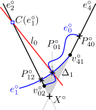
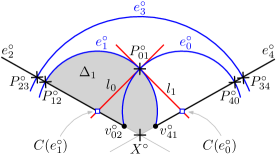
We now assume for a contradiction that the arc ${e}^{\circ}_{1}$ forms a concave side of the triangle $\Delta_{1}={P}^{\circ}_{12}{v}^{\circ}_{41}{X}^{\circ}$; see Figure 8(a) where the triangle is filled gray. (Symmetrically, we can show that the arc ${e}^{\circ}_{0}$ cannot form a concave side of the triangle $\Delta_{0}={P}^{\circ}_{40}{v}^{\circ}_{02}{X}^{\circ}$.) By Observation 1, $C({{e}^{\circ}_{1}})$ must lie on the ray ${e}^{\circ}_{2}$. Since we assume that the arc ${e}^{\circ}_{1}$ forms a concave side of the triangle $\Delta_{1}$, $C({{e}^{\circ}_{1}})$ and ${v}^{\circ}_{02}$ are separated by ${P}^{\circ}_{12}$ on ${e}^{\circ}_{2}$. Consider the tangent $l_{0}$ to ${e}^{\circ}_{0}$ at ${P}^{\circ}_{01}$. Again in light of Observation 1, $l_{0}$ has to go through $C({{e}^{\circ}_{1}})$ because ${e}^{\circ}_{0}$ and ${e}^{\circ}_{1}$ are orthogonal. On the one hand, ${v}^{\circ}_{02}$ is to the same side of $l_{0}$ as ${P}^{\circ}_{12}$; see Figure 8(a). On the other hand, $l_{0}$ separates ${P}^{\circ}_{12}$ and ${v}^{\circ}_{41}$ due to $\Pi({e_{1}};{e_{4},e_{0},e_{2}})$. Moreover, $l_{0}$ does not separate ${v}^{\circ}_{41}$ and ${P}^{\circ}_{40}$ since it intersects the line of ${e}^{\circ}_{4}$ when leaving the gray triangle $\Delta_{1}$. So the two points ${v}^{\circ}_{02}$ and ${P}^{\circ}_{40}$ of the same arc ${e}^{\circ}_{0}$ are separated by $l_{0}$, which is a tangent of this arc; contradiction.

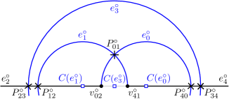
Thus, the arc ${e}^{\circ}_{1}$ forms a convex side of the triangle $\Delta_{1}$, and ${e}^{\circ}_{0}$ forms a convex side of $\Delta_{0}$; see Figure 8(b). Now, due to Observation 1, $C({{e}^{\circ}_{0}})$ is between ${v}^{\circ}_{41}$ and ${P}^{\circ}_{40}$, and $C({{e}^{\circ}_{1}})$ is between ${v}^{\circ}_{02}$ and ${P}^{\circ}_{12}$, because that is where the tangents $l_{1}$ of ${e}^{\circ}_{1}$ and $l_{0}$ of ${e}^{\circ}_{0}$ in ${P}^{\circ}_{01}$ intersect the lines of ${e}^{\circ}_{4}$ and ${e}^{\circ}_{2}$, respectively. Taking into account that $C({{e}^{\circ}_{3}})={X}^{\circ}$, because ${e}^{\circ}_{3}$ is orthogonal to both ${e}^{\circ}_{2}$ and ${e}^{\circ}_{4}$, we obtain that the points $C({{e}^{\circ}_{3}})$, $C({{e}^{\circ}_{1}})$, ${P}^{\circ}_{12}$, ${P}^{\circ}_{23}$ appear on the line of ${e}^{\circ}_{2}$ in this order. Thus, the circle of ${e}^{\circ}_{1}$ is contained within the circle of ${e}^{\circ}_{3}$. This is a contradiction because ${e}^{\circ}_{3}$ and ${e}^{\circ}_{1}$ must share a point; namely ${v}^{\circ}_{13}$.

Case II: $e_{2}$ and $e_{4}$ belong to the same circle.

Here ${e}^{\circ}_{2}$ and ${e}^{\circ}_{4}$ are two disjoint straight-line rays on the same line $l$ (meeting at infinity at ${v}^{\circ}_{24}$); see Figure 9. We direct $l$ as ${e}^{\circ}_{4}$ and ${e}^{\circ}_{2}$ (from right to left in Figure 9). Because ${e}^{\circ}_{0}$, ${e}^{\circ}_{1}$, and ${e}^{\circ}_{3}$ are orthogonal to $l$, their centers have to be on $l$. Due to our initial assumption, we have $\Pi({e_{4}};{e_{2},e_{3},e_{0},e_{1}})$ and $\Pi({e_{2}};{e_{0},e_{1},e_{3},e_{4}})$. Hence, along $l$, we have ${P}^{\circ}_{34}$, ${P}^{\circ}_{40}$, ${v}^{\circ}_{41}$, (on ${e}^{\circ}_{4}$) and then ${v}^{\circ}_{02}$, ${P}^{\circ}_{12}$, ${P}^{\circ}_{23}$ (on ${e}^{\circ}_{2}$). Therefore, the circle of ${e}^{\circ}_{1}$ is contained in that of ${e}^{\circ}_{3}$. Hence, ${e}^{\circ}_{1}$ does not share a point with ${e}^{\circ}_{3}$; a contradiction.

Figure 9: Illustration to the proof of Lemma 2.14 when $e_{2}$ and $e_{4}$ belong to the same circle. Image of the inversion with respect to the red circle in Figure 7(b).

Lemma 2.16.

A 0-pentagon in a simplified arc-RAC drawing contributes charge to at most three triangles.

Proof 2.17.

As discussed above, if a 0-pentagon formed by edges $e_{0},e_{1},\dots,e_{4}$ contributes charge to more than three triangles in a simplified drawing (see Figure 7(a)), then this implies the existence of an arc-RAC drawing where it holds that $\Pi({e_{0}};{e_{4},e_{1},e_{2}})$, $\Pi({e_{3}};{e_{1},e_{2},e_{4}})$ and, for $i\in\{1,2,4\}$, $\Pi({e_{i}};{e_{i-2},e_{i-1},e_{i+1},e_{i+2}})$; see Figure 7(b). This, however, contradicts Lemma 2.14.

With the proofs of Lemmas 2.8 and 2.16 now in place, the proof of Theorem 2.6 is complete.

3 A Lower Bound for the Maximum Edge Density

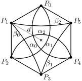
In this section, we construct a family of arc-RAC graphs with high edge density. Our construction is based on a family of RAC₁ graphs of high edge density that Arikushi et al. [6] constructed. Let $G$ be an embedded graph whose vertices are the vertices of the hexagonal lattice clipped inside a rectangle; see Figure 10(a). The edges of $G$ are the edges of the lattice and, inside each hexagon that is bounded by the cycle $(P_{0},\ldots,P_{5})$, six additional edges $(P_{i},P_{i+2\bmod 6})$ for $i\in\{0,1,\dots,5\}$; see Figure 10(b). We refer to a part of the drawing made up of a single hexagon and its diagonals as a tile. In Theorem 3.5 below, we show that each hexagon can be drawn as a regular hexagon and its diagonals can be drawn as two sets of arcs $A=\{\alpha_{0},\alpha_{1},\alpha_{2}\}$ and $B=\{\beta_{0},\beta_{1},\beta_{2}\}$, so that the arcs in $A$ are pairwise orthogonal, the arcs in $B$ are pairwise non-crossing, and for each arc in $B$ intersecting another arc in $A$ the two arcs are orthogonal; we use this construction to establish the theorem. In particular, the arcs in $A$ form the 3-cycle $(P_{0},P_{2},P_{4})$, and the arcs in $B$ form the 3-cycle $(P_{1},P_{3},P_{5})$.

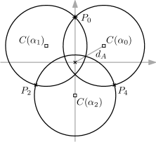
We first define the radii and centers of the arcs in a tile and show that they form only orthogonal crossings. We use the geometric center of the tile as the origin of our coordinate system in the following analysis. We now discuss the arcs in $A$; then we turn to the arcs in $B$. For each $j\in\{0,1,2\}$, the arc $\alpha_{j}$ has radius $r_{A}=1$ and center $C({\alpha_{j}})=(d_{A}\cos(\pi/6+j\frac{2\pi}{3}),d_{A}\sin(\pi/6+j\frac{2\pi}{3}))$, where $d_{A}=\sqrt{2/3}$ is the distance of the centers from the origin; see Figure 11(a).

Lemma 3.1.

The arcs in $A$ are pairwise orthogonal.

Proof 3.2.

Consider the equilateral triangle $\triangle C({\alpha_{0}})C({\alpha_{1}})C({\alpha_{2}})$ formed by the centers of the three arcs in $A$. Because the origin is in the center of the triangle, the edge length of the triangle is $2d_{A}\cos{\pi/6}=\sqrt{2}$, and so the distance between the centers of any two arcs is $\sqrt{2}$. The radii of the arcs are 1, hence by Observation 1, every two arcs are orthogonal.

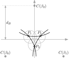
As in Figure 11(b), for each $j\in\{0,1,2\}$, the arc $\beta_{j}$ has radius $r_{B}=\sqrt{\frac{70+40\sqrt{3}}{6}}$ and center $C({\beta_{j}})=(d_{B}\cos(\frac{\pi}{2}+\frac{(j+1)2\pi}{3}),d_{B}\sin(\frac{\pi}{2}+\frac{(j+1)2\pi}{3}))$, where $d_{B}=\sqrt{\frac{1}{6}}+\sqrt{\frac{73+40\sqrt{3}}{6}}$ is the distance of the centers from the origin.

Lemma 3.3.

If an arc in $B$ intersects an arc in $A$, then the two arcs are orthogonal.

Proof 3.4.

Let $i,j\in\{0,1,2\}$. If $j\neq i$, $\|C({\alpha_{i}})-C({\beta_{j}})\|^{2}=\frac{76+40\sqrt{3}}{6}=1+\frac{70+40\sqrt{3}}{6}=r_{A}^{2}+r_{B}^{2}$, so by Observation 1 $\alpha_{i}$ and $\beta_{j}$ are orthogonal. Otherwise, for $i\in\{0,1,2\}$, $\|C({\alpha_{i}})-C({\beta_{i}})\|=\sqrt{\frac{112+64\sqrt{3}}{6}}>1+\sqrt{\frac{70+40\sqrt{3}}{6}}=r_{A}+r_{B}$, so $\alpha_{i}$ and $\beta_{i}$ do not intersect.

(a) The hexagonal lattice.

(b) A tile.

Figure 10: Tiling used for the lower-bound construction.

(a) Circles covering the arcs in $A$.

(b) Circles covering the arcs in $B$.

Figure 11: Construction for the lower bound on the maximum edge density of arc-RAC graphs.

Theorem 3.5.

For infinitely many values of $n$, there exists an $n$-vertex arc-RAC graph with $4.5n-O(\sqrt{n})$ edges.

Proof 3.6.

We first construct a tile and show that its drawing is indeed a valid arc-RAC drawing. Then it is easy to draw an embedded graph $G$ with the claimed edge density.

Consider two circles $\alpha$ and $\beta$ that intersect in two points of different distance from the origin. Let $X^{-}_{\alpha\beta}$ be the intersection point that is closer to the origin, and let $X^{+}_{\alpha\beta}$ be the intersection point further from the origin.

Let the vertices of the hexagon in a tile be $P_{0}=X^{+}_{\alpha_{0}\alpha_{1}}$, $P_{1}=X^{-}_{\beta_{2}\beta_{0}}$, $P_{2}=X^{+}_{\alpha_{1}\alpha_{2}}$, $P_{3}=X^{-}_{\beta_{0}\beta_{1}}$, $P_{4}=X^{+}_{\alpha_{2}\alpha_{0}}$, and $P_{5}=X^{-}_{\beta_{1}\beta_{2}}$. Due to the symmetric definitions of the arcs, the angle between two consecutive vertices of the hexagon is $\pi/3$. Moreover, by a simple computation, we see that for each $j\in\{0,1,2\}$ and with $d=\sqrt{1/2}+\sqrt{1/6}$ being the distance of the vertices of the hexagon from the origin, we have:

$$\begin{array}[]{l@{\;=\;}l@{\;=\;}l}P_{2j}&X^{+}_{\alpha_{j}\alpha_{j+1\bmod 3}}&\big{(}d\cos(\frac{\pi}{2}+j\frac{2\pi}{3}),\,d\sin(\frac{\pi}{2}+j\frac{2\pi}{3})\big{)}\\ P_{2j+3\bmod 6}&X^{-}_{\beta_{j}\beta_{j+1\bmod 3}}&\big{(}d\cos(\frac{\pi}{6}+(j+2)\frac{2\pi}{3}),\,d\sin(\frac{\pi}{6}+(j+2)\frac{2\pi}{3})\big{)}.\end{array}$$

Thus, all the vertices of the hexagon are equidistant from its center, so the hexagon is regular. According to Lemmas 3.1 and 3.3 all crossings of the arcs that belong to the same tile are orthogonal. Now we argue that the arcs in $A$ and $B$ are contained in the regular hexagon. To this end, we show that the arcs do not intersect the relative interior of the edges of the hexagon. To see this, take, for example, the arc $\alpha_{2}$, which connects $P_{2}$ and $P_{4}$. The line segment $P_{2}P_{4}$ is orthogonal to the side $P_{1}P_{2}$ of the hexagon. As the center of $\alpha_{2}$ is below $P_{2}P_{4}$, the tangent of $\alpha_{2}$ in $P_{2}$ enters the interior of the hexagon in $P_{2}$. Thus, $\alpha_{2}$ does not intersect the relative interior of the edge $P_{1}P_{2}$ (or of any other edge) of the hexagon. Similarly we can show that the arcs in $B$ do not intersect the relative interior of an edge of the hexagon. Therefore, each tile is an arc-RAC drawing, and $G$ is an arc-RAC graph.

Almost all vertices of the lattice with the exception of at most $O(\sqrt{n})$ vertices at the lattice’s boundary have degree 9 [6]. Hence $G$ has $4.5n-O(\sqrt{n})$ edges.

As any $n$-vertex RAC graph has at most $4n-10$ edges [13], we obtain the following.

Corollary 3.7.

The arc-RAC graphs are a proper superclass of the RAC₀ graphs.

4 Open Problems and Conjectures

An obvious open problem is to tighten the bounds on the edge density of arc-RAC graphs in Theorems 2.6 and 3.5.

Another immediate question is the relation to RAC₁ graphs, which also extend the class of RAC₀ graphs. This is especially intriguing as the best known lower bound for the maximum edge density of RAC₁ graphs is indeed larger than our lower bound for arc-RAC graphs whereas there may be arc-RAC graphs that are denser than the densest RAC₁ graphs.

The relation between RAC_k graphs and 1-planar graphs is well understood [6, 7, 8, 9, 11, 16]. What about the relation between arc-RAC graphs and 1-planar graphs? In particular, is there a 1-planar graph which is not arc-RAC?

We are also interested in the area required by arc-RAC drawings. Are there arc-RAC graphs that need exponential area to admit an arc-RAC drawing? (A way to measure this off the grid is to consider the ratio between the longest and the shortest edge in a drawing.)

Finally, the complexity of recognizing arc-RAC graphs is open, but likely NP-hard.

References

- [1] Eyal Ackerman. On the maximum number of edges in topological graphs with no four pairwise crossing edges. Discrete Comput. Geom., 41(3):365–375, 2009. doi:10.1007/s00454-009-9143-9.
- [2] Eyal Ackerman and Gábor Tardos. On the maximum number of edges in quasi-planar graphs. J. Combin. Theory, Ser. A, 114(3):563–571, 2007. doi:10.1016/j.jcta.2006.08.002.
- [3] Oswin Aichholzer, Wolfgang Aigner, Franz Aurenhammer, Kateřina Čech Dobiášová, Bert Jüttler, and Günter Rote. Triangulations with circular arcs. In Marc van Kreveld and Bettina Speckmann, editors, Proc. Graph Drawing (GD’11), volume 7034 of LNCS, pages 296–307. Springer, 2012. doi:10.1007/978-3-642-25878-7_29.
- [4] Patrizio Angelini, Michael A. Bekos, Henry Förster, and Michael Kaufmann. On RAC drawings of graphs with one bend per edge. In Therese Biedl and Andreas Kerren, editors, Proc. Graph Drawing & Network Vis. (GD’18), volume 11282 of LNCS, pages 123–136. Springer, 2018. doi:10.1007/978-3-030-04414-5_9.
- [5] Karin Arikushi, Radoslav Fulek, Baláazs Keszegh, Filip Morić, and Csaba D. Tóth. Graphs that admit right angle crossing drawings. In Dimitrios M. Thilikos, editor, Proc. Graph Theoretic Concepts in Comput. Sci. (WG’10), volume 6410 of LNCS, pages 135–146. Springer, 2010. doi:10.1007/978-3-642-16926-7_14.
- [6] Karin Arikushi, Radoslav Fulek, Baláazs Keszegh, Filip Morić, and Csaba D. Tóth. Graphs that admit right angle crossing drawings. Comput. Geom., 45(4):169–177, 2012. doi:10.1016/j.comgeo.2011.11.008.
- [7] Christian Bachmaier, Franz J. Brandenburg, Kathrin Hanauer, Daniel Neuwirth, and Josef Reislhuber. NIC-planar graphs. Discrete Appl. Math., 232:23–40, 2017. doi:10.1016/j.dam.2017.08.015.
- [8] Michael A. Bekos, Walter Didimo, Giuseppe Liotta, Saeed Mehrabi, and Fabrizio Montecchiani. On RAC drawings of 1-planar graphs. Theoretical Comput. Sci., 689:48–57, 2017. doi:10.1016/j.tcs.2017.05.039.
- [9] Franz J. Brandenburg, Walter Didimo, William S. Evans, Philipp Kindermann, Giuseppe Liotta, and Fabrizio Montecchiani. Recognizing and drawing IC-planar graphs. Theoret. Comput. Sci., 636:1–16, 2016. URL: https://arxiv.org/abs/1509.00388, doi:10.1016/j.tcs.2016.04.026.
- [10] Steven Chaplick, Henry Förster, Myroslav Kryven, and Alexander Wolff. On arrangements of orthogonal circles. In Daniel Archambault and Csaba D. Tóth, editors, Proc. Graph Drawing and Network Visualization (GD’19), volume 11904 of LNCS, pages 216–229. Springer, 2019. URL: https://arxiv.org/abs/1907.08121, doi:10.1007/978-3-030-35802-0_17.
- [11] Steven Chaplick, Fabian Lipp, Alexander Wolff, and Johannes Zink. Compact drawings of 1-planar graphs with right-angle crossings and few bends. Comput. Geom., 84:50–68, 2019. Special issue on EuroCG 2018. doi:10.1016/j.comgeo.2019.07.006.
- [12] C. C. Cheng, Christian A. Duncan, Michael T. Goodrich, and Stephen G. Kobourov. Drawing planar graphs with circular arcs. Discrete Comput. Geom., 25:405–418, 2001. doi:10.1007/s004540010080.
- [13] Walter Didimo, Peter Eades, and Giuseppe Liotta. Drawing graphs with right angle crossings. Theoret. Comput. Sci., 412(39):5156–5166, 2011. doi:10.1016/j.tcs.2011.05.025.
- [14] Walter Didimo, Giuseppe Liotta, and Fabrizio Montecchiani. A survey on graph drawing beyond planarity. ACM Comput. Surv., 52(1):4:1–4:37, 2019. doi:10.1145/3301281.
- [15] Vida Dujmović, Joachim Gudmundsson, Pat Morin, and Thomas Wolle. Notes on large angle crossing graphs. In A. Potanin and A. Viglas, editors, Proc. Comput. Australasian Theory Symp. (CATS’10), volume 109 of CRPIT, pages 19–24. Australian Computer Society, 2010. URL: http://dl.acm.org/citation.cfm?id=1862317.1862320.
- [16] Peter Eades and Giuseppe Liotta. Right angle crossing graphs and 1-planarity. Discrete Appl. Math., 161(7):961–969, 2013. doi:10.1016/j.dam.2012.11.019.
- [17] Weidong Huang. Using eye tracking to investigate graph layout effects. In Seok-Hee Hong and Kwan-Liu Ma, editors, Proc. Asia-Pacific Symp. Visual. (APVIS’07), pages 97–100. IEEE, 2007. doi:10.1109/APVIS.2007.329282.
- [18] Weidong Huang, Peter Eades, and Seok-Hee Hong. Larger crossing angles make graphs easier to read. J. Vis. Lang. Comput., 25(4):452–465, 2014. doi:10.1016/j.jvlc.2014.03.001.
- [19] Weidong Huang, Seok-Hee Hong, and Peter Eades. Effects of crossing angles. In Proc. IEEE VGTC Pacific Visualization (PacificVis’08), pages 41–46, 2008. doi:10.1109/PACIFICVIS.2008.4475457.
- [20] Michael Jünger and Petra Mutzel, editors. Graph Drawing Software. Springer, Berlin, Heidelberg, 2004. doi:10.1007/978-3-642-18638-7.
- [21] Michael Kaufmann and Dorothea Wagner, editors. Drawing Graphs: Methods and Models. Springer, Berlin, Heidelberg, 2001. doi:10.1007/3-540-44969-8.
- [22] Myroslav Kryven, Alexander Ravsky, and Alexander Wolff. Drawing graphs on few circles and few spheres. J. Graph Algorithms Appl., 23(2):371–391, 2019. doi:10.7155/jgaa.00495.
- [23] Mark Lombardi and Robert Hobbs, editors. Mark Lombardi: Global Networks. Independent Curators, 2003.
- [24] C. Stanley Ogilvy. Excursions in Geometry. Oxford Univ. Press, New York, 1969.
- [25] János Pach, Radoš Radoičić, and Géza Tóth. Relaxing planarity for topological graphs. In Ervin Győri, Gyula O. H. Katona, László Lovász, and Tamás Fleiner, editors, More Sets, Graphs and Numbers: A Salute to Vera Sós and András Hajnal, pages 285–300. Springer Berlin Heidelberg, 2006. doi:10.1007/978-3-540-32439-3_12.
- [26] Helen C. Purchase, John Hamer, Martin Nöllenburg, and Stephen G. Kobourov. On the usability of Lombardi graph drawings. In Walter Didimo and Maurizio Patrignani, editors, Proc. Graph Drawing (GD’12), volume 7704 of LNCS, pages 451–462. Springer, 2013. doi:10.1007/978-3-642-36763-2_40.
- [27] André Schulz. Drawing graphs with few arcs. J. Graph Algorithms Appl., 19(1):393–412, 2015. doi:10.7155/jgaa.00366.
- [28] Kai Xu, Chris Rooney, Peter Passmore, and Dong-Han Ham. A user study on curved edges in graph visualisation. In Philip Cox, Beryl Plimmer, and Peter Rodgers, editors, Proc. Theory Appl. Diagrams (DIAGRAMS’10), volume 7352 of LNCS, pages 306–308. Springer, 2012. doi:10.1007/978-3-642-31223-6_34.