On the Co-Design of AV-Enabled Mobility Systems

Abstract

The design of autonomous vehicles (AVs) and the design of AV-enabled mobility systems are closely coupled. Indeed, knowledge about the intended service of AVs would impact their design and deployment process, whilst insights about their technological development could significantly affect transportation management decisions. This calls for tools to study such a coupling and co-design AVs and AV-enabled mobility systems in terms of different objectives. In this paper, we instantiate a framework to address such co-design problems. In particular, we leverage the recently developed theory of co-design to frame and solve the problem of designing and deploying an intermodal Autonomous Mobility-on-Demand system, whereby AVs service travel demands jointly with public transit, in terms of fleet sizing, vehicle autonomy, and public transit service frequency. Our framework is modular and compositional, allowing one to describe the design problem as the interconnection of its individual components and to tackle it from a system-level perspective. To showcase our methodology, we present a real-world case study for Washington D.C., USA. Our work suggests that it is possible to create user-friendly optimization tools to systematically assess costs and benefits of interventions, and that such analytical techniques might gain a momentous role in policy-making in the future.

I Introduction

Arguably, the current design process for AVs largely suffers from the lack of clear, specific requirements in terms of the service such vehicles will be providing. Yet, knowledge about their intended service (e.g., last-mile versus point-to-point travel) might dramatically impact how the AVs are designed, and, critically, significantly ease their development process. For example, if for a given city we knew that for an effective on-demand mobility system autonomous cars only need to drive up to 25 mph and only on relatively easy roads, their design would be greatly simplified and their deployment could certainly be accelerated. At the same time, from the system-level perspective of transportation management, knowledge about the trajectory of technology development for AVs would certainly impact decisions on infrastructure investments and provision of service. In other words, the design of the AVs and the design of a mobility system leveraging AVs are intimately coupled. This calls for methods to reason about such a coupling, and in particular to co-design the AVs and the associated AV-enabled mobility system. A key requirement in this context is the ability to account for a range of heterogeneous objectives that are often not directly comparable (consider, for instance, travel time and emissions).

Accordingly, the goal of this paper is to lay the foundations for a framework through which one can co-design future AV-enabled mobility systems. Specifically, we show how one can leverage the recently developed mathematical theory of co-design [2, 3, 4], which provides a general methodology to co-design complex systems in a modular and compositional fashion. This tool delivers the set of rational design solutions lying on the Pareto front, allowing one to reason about costs and benefits of the individual design options. The framework is instantiated in the setting of co-designing intermodal AMoD systems [5], whereby fleets of self-driving vehicles provide on-demand mobility jointly with public transit. Aspects subject to co-design include fleet size, AV-specific characteristics, and public transit service frequency.

I-A Literature Review

Our work lies at the interface of the design of urban public transportation services and the design of AMoD systems. The first research stream is reviewed in [6, 7], and comprises strategic long-term infrastructure modifications and operational short-term scheduling. The joint design of traffic network topology and control infrastructure has been presented in [8]. Public transportation scheduling has been solved jointly with the design of the transit network in a passengers’ and operators’ cost-optimal fashion in [9], using demand-driven approaches in [10], and in an energy-efficient way in [11]. However, these works only focus on the public transit system and do not consider its joint design with an AMoD system. The research on the design of AMoD systems is reviewed in [12] and mainly pertains their fleet sizing. In this regard, studies range from simulation-based approaches [13, 14, 15, 16] to analytical methods [17]. In [18], the authors jointly design the fleet size and the charging infrastructure, and formulate the arising design problem as a mixed integer linear program. The authors of [19] solve the fleet sizing problem together with the vehicle allocation problem. Finally, [20] co-designs the AMoD fleet size and its composition. More recently, the joint design of multimodal transit networks and AMoD systems was formulated in [21] as a bilevel optimization problem and solved with heuristics. Overall, the problem-specific structure of existing design methods for AMoD systems is not amenable to a modular and compositional problem formulation. Moreover, previous work does not capture important aspects of AV-enabled mobility systems, such as other transportation modes and AV-specific design parameters (e.g., the level of autonomy).

I-B Statement of Contribution

In this paper we lay the foundations for the systematic study of the design of AV-enabled mobility systems. Specifically, we leverage the mathematical theory of co-design [2] to devise a framework to study the design of intermodal AMoD (I-AMoD) systems in terms of fleet characteristics and public transit service, enabling the computation of the rational solutions lying on the Pareto front of minimal travel time, transportation costs, and emissions. Our framework allows one to structure the design problem in a modular way, in which each different transportation option can be “plugged in” in a larger model. Each model has minimal assumptions: Rather than properties such as linearity and convexity, we ask for very general monotonicity assumptions. For example, we assume that the cost of automation increases monotonically with the speed achievable by the AV. We are able to obtain the full Pareto front of rational solutions, or, given policies, to weigh incomparable costs (such as travel time and emissions) and to present actionable information to the stakeholders of the mobility ecosystem. We showcase our methodology through a real-world case study of Washington D.C., USA. We show how, given the model, we can easily formulate and answer several questions regarding the introduction of new technologies and investigate possible infrastructure interventions.

I-C Organization

The remainder of this paper is structured as follows: Section II reviews the mathematical theory of co-design. Section III presents the co-design problem for AV-enabled mobility systems. We showcase our approach with real-world case studies for Washington D.C., USA, in Section IV. Section V concludes the paper with a discussion and an overview on future research directions.

II Background

This paper builds on the mathematical theory of co-design, presented in [2]. In this section, we present a review of the main contents needed for this work.

II-A Orders

We will use basic facts from order theory, which we review in the following.

Definition II.1 (Poset).

A partially ordered set (poset) is a tuple $\langle\mathcal{P},\preceq_{\mathcal{P}}\rangle$, where $\mathcal{P}$ is a set and $\preceq_{\mathcal{P}}$ is a partial order, defined as a reflexive, transitive, and antisymmetric relation.

Given a poset, we can formalize the idea of “Pareto front” through antichains.

Definition II.2 (Antichains).

A subset $S\subseteq\mathcal{P}$ is an antichain iff no elements are comparable: For $x,y\in S$, $x\preceq y$ implies $x=y$. We denote by $\textsf{A}\mathcal{P}$ the set of all antichains in $\mathcal{P}$.

Definition II.3 (Directed set).

A subset $S\subseteq\mathcal{P}$ is directed if each pair of elements in $S$ has an upper bound: For all $a,b\in S$, there exists a $c\in S$ such that $a\preceq c$ and $b\preceq c$.

Definition II.4 (Completeness).

A poset is a complete partial order (CPO) if each of its directed subsets has a supremum and a least element.

For instance, the poset $\langle\mathbb{R}_{+},\leq\rangle$, with $\mathbb{R}_{+}\coloneqq\{x\in\mathbb{R}\,|\,x\geq 0\}$, is not complete, as its directed subset $\mathbb{R}_{+}\subseteq\mathbb{R}_{+}$ does not have an upper bound (and therefore a supremum). Nonetheless, we can make it complete by artificially adding a top element $\top$, i.e., by defining $\langle\overline{\mathbb{R}}_{+},\leq\rangle$ with $\overline{\mathbb{R}}_{+}\coloneqq\mathbb{R}_{+}\cup\{\top\}$ and $a\leq\top$ for all $a\in\mathbb{R}_{+}$. Similarly, we can complete $\mathbb{N}$ to $\overline{\mathbb{N}}$.

In this setting, Scott-continuous maps will play a key role. Intuitively, Scott-continuity can be understood as a stronger notion of monotonicity.

Definition II.5 (Scott continuity).

A map $f:\mathcal{P}\rightarrow\mathcal{Q}$ between two posets $\langle\mathcal{P},\preceq_{\mathcal{P}}\rangle$ and $\langle\mathcal{Q},\preceq_{\mathcal{Q}}\rangle$ is Scott-continuous iff for each directed set $D\subseteq\mathcal{P}$ the image $f(D)$ is directed and $\sup f(D)=f(\sup D)$.

II-B Mathematical Theory of Co-Design

We start by presenting design problems with implementation (DPIs), which can then be composed and interconnected to form a co-design problem with implementation (CDPI).

Definition II.6 (DPI).

A DPI is a tuple $\langle\mathcal{F},\mathcal{R},\mathcal{I},\textsf{{exe}},\textsf{{eva}}\rangle$:

• $\mathcal{F}$ is a poset, called functionality space;

• $\mathcal{R}$ is a poset, called resource space;

• $\mathcal{I}$ is a set, called implementation space;

• the map $\textsf{{exe}}:\mathcal{I}\to\mathcal{F}$ maps an implementation to the functionality it provides;

• the map $\textsf{{eva}}:\mathcal{I}\to\mathcal{R}$, maps an implementation to the resources it requires.

Given a DPI we can define a map which, given a functionality $\textsf{{f}}\in\mathcal{F}$, returns all the non-comparable resources (i.e., the antichain) which provide f.

Definition II.7 (Functionality to resources map).

Given a DPI $\langle\mathcal{F},\mathcal{R},\mathcal{I},\textsf{{exe}},\textsf{{eva}}\rangle$ define the map $h:\mathcal{F}\to\textsf{{A}}\mathcal{R}$ as

$$h: \mathcal{F} \to \textsf{{A}}\mathcal{R}$$ (1)

f $$\mapsto \min_{\preceq_{\mathcal{R}}}\{\textsf{{eva}}(\textsf{{i}})\,|\,\textsf{{i}}\in\mathcal{I}\wedge\textsf{{f}}\preceq\textsf{{exe}}(\textsf{{i}})\}.$$

In particular, if a functionality is infeasible, then $h(\textsf{{f}})=\emptyset$. We now turn our attention to “monotone” DPIs.

Definition II.8 (Monotone DPI).

We say a DPI $\langle\mathcal{F},\mathcal{R},\mathcal{I},\textsf{{exe}},\textsf{{eva}}\rangle$ is monotone if:

1. The posets $\mathcal{F}$ and $\mathcal{R}$ are CPOs.

2. The map $h$ (see Definition II.7) is Scott-continuous.

Individual DPIs can be composed in series (i.e., the functionality of a DPI is the resource of a second DPI) and in parallel (i.e., two DPIs share the same resource or functionality) to obtain a CDPI. Notably, such compositions preserve monotonicity and, thus, all related algorithmic properties. For further details we refer to [2].

III Co-Design of AV-enabled Mobility Systems

III-A Intermodal AMoD Framework

III-A1 Multi-Commodity Flow Model

The transportation system and its different modes are modeled using the digraph $\mathcal{G}=\left(\mathcal{V},\mathcal{A}\right)$, shown in Footnote 2.

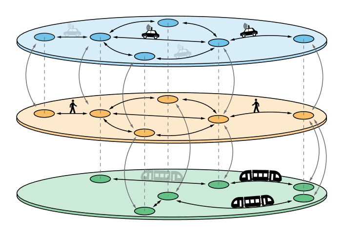
Figure 1: The I-AMoD network consists of a road, a walking, and a public transportation digraph. The coloured circles represent stops or intersections and the black arrows denote road links, pedestrian pathways, or public transit arcs. Dashed lines are nodes which are close geographically, while grey arrows denote the mode-switching arcs connecting them.

It is described through a set of nodes $\mathcal{V}$ and a set of arcs $\mathcal{A}\subseteq\mathcal{V}\times\mathcal{V}$. Specifically, it contains a road network layer $\mathcal{G}_{\mathrm{R}}=\left(\mathcal{V}_{\mathrm{R}},\mathcal{A}_{\mathrm{R}}\right)$, a public transportation layer $\mathcal{G}_{\mathrm{P}}=\left(\mathcal{V}_{\mathrm{P}},\mathcal{A}_{\mathrm{P}}\right)$, and a walking layer $\mathcal{G}_{\mathrm{W}}=\left(\mathcal{V}_{\mathrm{W}},\mathcal{A}_{\mathrm{W}}\right)$. The road network is characterized through intersections $i\in\mathcal{V}_{\mathrm{R}}$ and road segments $(i,j)\in\mathcal{A}_{\mathrm{R}}$. Similarly, public transportation lines are modeled through station nodes $i\in\mathcal{V}_{\mathrm{P}}$ and line segments $(i,j)\in\mathcal{A}_{\mathrm{P}}$. The walking network contains walkable streets $(i,j)\in\mathcal{A}_{\mathrm{W}}$, connecting intersections $i\in\mathcal{V}_{\mathrm{W}}$. Our model allows mode-switching arcs $\mathcal{A}_{\mathrm{C}}\subseteq\mathcal{V}_{\mathrm{R}}\times\mathcal{V}_{\mathrm{W}}\cup\mathcal{V}_{\mathrm{W}}\times\mathcal{V}_{\mathrm{R}}\cup\mathcal{V}_{\mathrm{P}}\times\mathcal{V}_{\mathrm{W}}\cup\mathcal{V}_{\mathrm{W}}\times\mathcal{V}_{\mathrm{P}}$, connecting the road and the public transportation layers to the walking layer. Consequently, $\mathcal{V}=\mathcal{V}_{\mathrm{W}}\cup\mathcal{V}_{\mathrm{R}}\cup\mathcal{V}_{\mathrm{P}}$ and $\mathcal{A}=\mathcal{A}_{\mathrm{W}}\cup\mathcal{A}_{\mathrm{R}}\cup\mathcal{A}_{\mathrm{P}}\cup\mathcal{A}_{\mathrm{C}}$. Consistently with the structural properties of road and walking networks in urban environments, we assume the graph $\mathcal{G}$ to be strongly connected. We represent customer movements by means of travel requests. A travel request refers to a customer flow starting its trip at a node $o\in\mathcal{V}$ and ending it at a node $d\in\mathcal{V}$.

Definition III.1 (Travel request).

A travel request $\rho$ is a triple $(o,d,\alpha)\in\mathcal{V}\times\mathcal{V}\times\mathbb{R}_{+}$, described by an origin node $o\in\mathcal{V}$, a destination node $d\in\mathcal{V}$, and the request rate $\alpha>0$, namely, the number of customers who want to travel from $o$ to $d$ per unit time.

To ensure that a customer is not forced to use a given transportation mode, we assume all requests to lie on the walking digraph, i.e., $o_{m},d_{m}\in\mathcal{V}_{\mathrm{W}}$ for all $m\in\mathcal{M}\coloneqq\{1,\ldots,M\}$.

The flow $f_{m}\left(i,j\right)\geq 0$ represents the number of customers per unit time traversing arc $(i,j)\in\mathcal{A}$ and satisfying a travel request $m$. Furthermore, $f_{0}\left(i,j\right)\geq 0$ denotes the flow of empty AVs on road arcs $(i,j)\in\mathcal{A}_{\mathrm{R}}$. This accounts for rebalancing flows of AVs between a customer’s drop-off and the next customer’s pick-up. Assuming AVs to carry one customer at a time, the flows satisfy

$$\sum_{i:(i,j)\in\mathcal{A}}f_{m}\left(i,j\right)+\mathds{1}_{j=o_{m}}\cdot\alpha_{m}=\sum_{k:(j,k)\in\mathcal{A}}f_{m}\left(j,k\right)+\mathds{1}_{j=d_{m}}\cdot\alpha_{m}$$

$$\hskip 136.5733pt\forall m\in\mathcal{M},\,j\in\mathcal{V}$$ (2a)

$$\sum_{i:(i,j)\in\mathcal{A}_{\mathrm{R}}}f_{\mathrm{tot}}\left(i,j\right)=\sum_{k:(j,k)\in\mathcal{A}_{\mathrm{R}}}f_{\mathrm{tot}}\left(j,k\right)\quad\forall j\in\mathcal{V}_{\mathrm{R}},$$ (2b)

where $\mathbb{1}_{j=x}$ denotes the boolean indicator function and $f_{\mathrm{tot}}\left(i,j\right)\coloneqq f_{0}\left(i,j\right)+\sum_{m\in\mathcal{M}}f_{m}\left(i,j\right)$. Specifically, (2a) guarantees flows conservation for every transportation demand, and (2b) preserves flow conservation for AVs on every road node. Combining conservation of customers (2a) with the conservation of AVs (2b) guarantees rebalancing AVs to match the demand.

III-B Travel Time and Travel Speed

The variable $t_{ij}$ denotes the time needed to traverse an arc $(i,j)$ of length $s_{ij}$. We assume a constant walking speed on walking arcs and infer travel times on public transportation arcs from the public transit schedules. Assuming that the public transportation system at node $j$ operates with frequency $\varphi_{j}$, switching from a pedestrian vertex $i\in\mathcal{V}_{\mathrm{W}}$ to a public transit station $j\in\mathcal{V}_{\mathrm{P}}$ takes, on average,

$$t_{ij}=t_{\mathrm{WS}}+0.5\cdot 1/\varphi_{j}\quad\forall(i,j)\in\mathcal{A}_{\mathrm{W}},$$ (3)

where $t_{\mathrm{WS}}$ is a constant sidewalk-to-station travel time. We assume that the average waiting time for AMoD vehicles is $t_{\mathrm{WR}}$, and that switching from the road graph and the public transit graph to the walking graph takes the transfer times $t_{\mathrm{RW}}$ and $t_{\mathrm{SW}}$, respectively. While each road arc $(i,j)\in\mathcal{A}_{\mathrm{R}}$ is characterized by a speed limit $v_{\mathrm{L,V},ij}$, AVs safety protocols impose a maximum achievable velocity $v_{\mathrm{V,a}}$. In order to prevent too slow and therefore dangerous driving behaviours, we only consider road arcs through which the AVs can drive at least at a fraction $\beta$ of the speed limit: Arc $(i,j)\in\mathcal{A}_{\mathrm{R}}$ is kept in the road network iff

$$v_{\mathrm{V,a}}\geq\beta\cdot v_{\mathrm{L,V},ij},$$ (4)

where $\beta\in(0,1]$. We set the velocity of all arcs fulfilling condition (4) to $v_{\mathrm{V},ij}=\min\{v_{\mathrm{V,a}},v_{\mathrm{L,V},ij}\}$ and compute the travel time to traverse them as

$$t_{ij}=s_{ij}/v_{\mathrm{V},ij}\quad\forall(i,j)\in\mathcal{A}_{\mathrm{R}}.$$ (5)

III-C Road Congestion

We capture congestion effects with a threshold model. The total flow on each road arc $(i,j)\in\mathcal{A}_{\mathrm{R}}$, given by the sum of the AVs flow $f_{\mathrm{tot}}\left(i,j\right)$ and the baseline usage $u_{ij}$ (e.g., private vehicles), must remain below the nominal capacity $c_{ij}$ of the arc:

$$f_{\mathrm{tot}}\left(i,j\right)+u_{ij}\leq c_{ij}\quad\forall(i,j)\in\mathcal{A}_{\mathrm{R}}.$$ (6)

III-D Energy Consumption

We compute the energy consumption of AVs for each road link considering an urban driving cycle, scaled so that the average speed $v_{\mathrm{avg,cycle}}$ matches the free-flow speed on the link. The energy consumption is then scaled as

$$e_{ij}=e_{\mathrm{cycle}}\cdot s_{ij}/s_{\mathrm{cycle}}\quad\forall(i,j)\in\mathcal{A}_{\mathrm{R}}.$$ (7)

For the public transportation system, we assume a constant energy consumption per unit time. This approximation is reasonable in urban environments, as the operation of the public transportation system is independent from the number of customers serviced, and its energy consumption is therefore customer-invariant.

III-E Fleet Size

We consider a fleet of $n_{\mathrm{V,max}}$ AVs. In a time-invariant setting, the number of vehicles on arc $(i,j)\in\mathcal{A}_{\mathrm{R}}$ is expressed as the product of the total vehicles flow on the arc and its travel time. Therefore, we constrain the number of used AVs as

$$n_{\mathrm{V,u}}=\sum_{(i,j)\in\mathcal{A}_{\mathrm{R}}}f_{\mathrm{tot}}\left(i,j\right)\cdot t_{ij}\leq n_{\mathrm{V,max}}.$$ (8)

III-F Discussion

A few comments are in order. First, we assume the demand to be time-invariant and allow flows to have fractional values. This assumption is in line with the mesoscopic and system-level planning perspective of our study. Second, we model congestion effects using a threshold model. This approach can be interpreted as a municipality preventing AVs to exceed the critical flow density on road arcs. AVs can be therefore assumed to travel at free-flow speed [22]. This assumption is realistic for an initial low penetration of AMoD systems in the transportation market, especially when the AV fleet is of limited size. Finally, we allow AVs to transport one customer at the time [23].

III-G Co-Design Framework

We integrate the I-AMoD framework presented in Section III-A in the co-design formalism, allowing one to decompose the CDPI of a complex system in the DPIs of its individual components in a modular, compositional, and systematic fashion. We aim at computing the antichain of resources, quantified in terms of costs, average travel time per trip, and emissions required to provide the mobility service to a set of customers. In order to achieve this, we decompose the CDPI in the DPIs of the individual AVs (Section III-G1), of the AV fleet (Section III-G3), and of the public transportation system (Section III-G2). The interconnection of the presented DPIs is presented in Section III-G4.

III-G1 The Autonomous Vehicle Design Problem

The AV DPI consists of selecting the maximal speed of the AVs. Under the rationale that driving safely at higher speed requires more advanced sensing and algorithmic capabilities, we model the achievable speed of the AVs $v_{\mathrm{V,a}}$ as a monotone function of the vehicle fixed costs $C_{\mathrm{V,f}}$ (resulting from the cost of the vehicle $C_{\mathrm{V,v}}$ and the cost of its automation $C_{\mathrm{V,a}}$) and of the mileage-dependent operational costs $C_{\mathrm{V,o}}$ (accounting for maintenance, cleaning, energy consumption, depreciation, and opportunity costs [24]). In this setting, the AV DPI provides the functionality $v_{\mathrm{V,a}}$ and requires the resources $C_{\mathrm{V,f}}$ and $C_{\mathrm{V,o}}$. Consequently, the functionality space is $\mathcal{F}_{\mathrm{V}}=\overline{\mathbb{R}}_{+}$, and the resources space is $\mathcal{R}_{\mathrm{V}}=\overline{\mathbb{R}}_{+}\times\overline{\mathbb{R}}_{+}$.

III-G2 The Subway Design Problem

We design the public transit infrastructure by means of the service frequency introduced in Section III-B. Specifically, we assume that the service frequency $\varphi_{j}$ scales linearly with the size of the train fleet $n_{\mathrm{S}}$ as

$$\varphi_{j}/\varphi_{j,\mathrm{base}}=n_{\mathrm{S}}/n_{\mathrm{S,base}}.$$ (9)

We relate a train fleet of size $n_{\mathrm{S}}$ to the fixed costs $C_{\mathrm{S,f}}$ (accounting for train and infrastructural costs) and to the operational costs $C_{\mathrm{S,o}}$ (accounting for energy consumption, vehicles depreciation, and train operators’ wages). Given the passenger-independent public transit operation in today’s cities, we reasonably assume the operational costs $C_{\mathrm{S,o}}$ to be mileage independent and to only vary with the size of the fleet. Formally, the number of acquired trains $n_{\mathrm{S,a}}=n_{\mathrm{S}}-n_{\mathrm{S,base}}$ is a functionality, whereas $C_{\mathrm{S,f}}$ and $C_{\mathrm{S,o}}$ are resources. The functionality space is $\mathcal{F}_{\mathrm{S}}=\overline{\mathbb{N}}$ and the resources space is $\mathcal{R}_{\mathrm{S}}=\overline{\mathbb{R}}_{+}\times\overline{\mathbb{R}}_{+}$.

III-G3 The I-AMoD Framework Design Problem

The I-AMoD DPI considers demand satisfaction as a functionality. Formally, $\mathcal{F}_{\mathrm{O}}=2^{\mathcal{V}\times\mathcal{V}\times\overline{\mathbb{R}}_{+}}$ with the partial order $\preceq_{\mathcal{F}_{\mathrm{O}}}$ defined by $\mathcal{D}_{1}\coloneqq\{(o^{1}_{i},d^{1}_{i},\alpha^{1}_{i})\}_{i=1}^{M_{1}}\preceq_{\mathcal{F}_{\mathrm{O}}}\{(o^{2}_{i},d^{2}_{i},\alpha^{2}_{i})\}_{i=1}^{M_{2}}\eqqcolon\mathcal{D}_{2}$ iff for all $(o^{1},d^{1},\alpha^{1})\in\mathcal{D}_{1}$ there is some $(o^{2},d^{2},\alpha^{2})\in\mathcal{D}_{2}$ with $o^{1}=o^{2}$, $d^{1}=d^{2}$, and $\alpha^{2}_{i}\geq\alpha^{1}_{i}$. In other words, $\mathcal{D}_{1}\preceq_{\mathcal{F}_{\mathrm{O}}}\mathcal{D}_{2}$ if every travel request in $\mathcal{D}_{1}$ is in $\mathcal{D}_{2}$ too. To successfully satisfy a given set of travel requests, we require the following resources: (i) the achievable speed of the AVs $v_{\mathrm{V,a}}$, (ii) the number of available AVs per fleet $n_{\mathrm{V,max}}$, (iii) the number of trains $n_{\mathrm{S,a}}$ acquired by the public transportation system, and (iv) the average travel time of a trip

$$t_{\mathrm{avg}}\coloneqq\frac{1}{\alpha_{\mathrm{tot}}}\cdot\sum_{m\in\mathcal{M},(i,j)\in\mathcal{A}}t_{ij}\cdot f_{m}\left(i,j\right),$$ (10)

with $\alpha_{\mathrm{tot}}\coloneqq\sum_{m\in\mathcal{M}}\alpha_{m}$, (v) the total distance driven by the AVs per unit time

$$s_{\mathrm{V,tot}}\coloneqq\sum_{(i,j)\in\mathcal{A}_{\mathrm{R}}}s_{ij}\cdot f_{\mathrm{tot}}\left(i,j\right),$$ (11)

(vi) the total AVs CO₂ emissions per unit time

$$m_{\mathrm{CO_{2},V,tot}}\coloneqq\gamma\cdot\sum_{(i,j)\in\mathcal{A}_{\mathrm{R}}}e_{ij}\cdot f_{\mathrm{tot}}\left(i,j\right),$$ (12)

where $\gamma$ relates the energy consumption and the CO₂ emissions. We assume that customers’ trips and AMoD rebalancing strategies are chosen to maximize customers’ welfare, defined through the average travel time $t_{\mathrm{avg}}$. Hence, we link the functionality and resources of the I-AMoD DPI through the following optimization problem:

$$\begin{split}\min_{\begin{subarray}{c}f_{m}\left(\cdot,\cdot\right)\geq 0,\\ f_{0}\left(\cdot,\cdot\right)\geq 0\end{subarray}}t_{\mathrm{avg}}&=\frac{1}{\alpha_{\mathrm{tot}}}\sum_{m\in\mathcal{M},(i,j)\in\mathcal{A}}t_{ij}\cdot f_{m}\left(i,j\right)\\ &\mathrm{s.t.\ Eq.}\eqref{eq:flowconstotal},\ \mathrm{Eq.}\eqref{eq:capacity},\ \mathrm{Eq.}\eqref{eq:fleetsizecar}.\end{split}$$ (13)

Formally, $\mathcal{F}_{\mathrm{O}}=\overline{\mathbb{R}}_{+}$, and $\mathcal{R}_{\mathrm{O}}=\overline{\mathbb{R}}_{+}\times\overline{\mathbb{N}}\times\overline{\mathbb{N}}\times\overline{\mathbb{R}}_{+}\times\overline{\mathbb{R}}_{+}\times\overline{\mathbb{R}}_{+}$.

Remark.

In general, the optimization problem (13) might possess multiple optimal solutions, making the relation between resources and functionality ill-posed. To overcome this subtlety, if two solutions share the same average travel time, we select the one incurring in the lowest mileage.

III-G4 The Monotone Co-Design Problem

The functionality of the system is to provide mobility service to the customers. Formally, the functionality provided by the CDPI is the set of travel requests. To provide the mobility service, the following three resources are required. First, on the customers’ side, we require an average travel time, defined in (10). Second, on the municipality side, the resource is the total transportation cost of the intermodal mobility system. Assuming an average vehicles’ life $l_{\mathrm{V}}$, an average trains’ life $l_{\mathrm{S}}$, and a baseline subway fleet of $n_{\mathrm{S,base}}$ trains, we express the total costs as

$$C_{\mathrm{tot}}=C_{\mathrm{V}}+C_{\mathrm{S}},$$ (14)

where $C_{\mathrm{V}}$ is the AV-related cost

$$C_{\mathrm{V}}=\frac{C_{\mathrm{V,f}}}{l_{\mathrm{V}}}\cdot n_{\mathrm{V,max}}+C_{\mathrm{V,o}}\cdot s_{\mathrm{V,tot}},$$ (15)

and $C_{\mathrm{S}}$ is the public transit-related cost

$$C_{\mathrm{S}}=\frac{C_{\mathrm{S,f}}}{l_{\mathrm{S}}}\cdot n_{\mathrm{S,a}}+C_{\mathrm{S,o}}.$$ (16)

Third, on the environmental side, the resources are the total CO₂ emissions

$$m_{\mathrm{CO_{2},tot}}=m_{\mathrm{CO_{2},V,tot}}+m_{\mathrm{CO_{2},S}}\cdot n_{\mathrm{S}},$$ (17)

where $m_{\mathrm{CO_{2},S}}$ represents the CO₂ emissions of a single train. Formally, the set of travel requests $\{\rho_{m}\}_{m\in\mathcal{M}}$ is the CDPI functionality, whereas $t_{\mathrm{avg}}$, $C_{\mathrm{tot}}$, and $m_{\mathrm{CO_{2},tot}}$ are its resources. Consistently, the functionality space is $\mathcal{F}=\overline{\mathbb{R}}_{+}$ and the resources space is $\mathcal{R}=\overline{\mathbb{R}}_{+}\times\overline{\mathbb{R}}_{+}\times\overline{\mathbb{R}}_{+}$. Note that the resulting CDPI (Figure 2) is indeed monotone, since it consists of the interconnection of monotone DPIs [2].

III-G5 Discussion

A few comments are in order. First, we lump the autonomy functionalities in its achievable velocity. We leave to future research more elaborated AV models, accounting for instance for accidents rates [25] and for safety levels. Second, we assume the service frequency of the subway system to scale linearly with the number of trains. We inherently rely on the assumption that the existing infrastructure can homogeneously accommodate the acquired train cars. To justify the assumption, we include an upper bound on the number of potentially acquirable trains in our case study design in Section IV. Third, we highlight that the I-AMoD framework is only one of the many feasible ways to map total demand to travel time, costs, and emissions. Specifically, practitioners can easily replace the corresponding DPI with more sophisticated models (e.g., simulation-based frameworks like AMoDeus [26]), as long as the monotonicity of the DPI is preserved. In our setting, we conjecture the customers’ and vehicles’ routes to be centrally controlled by the municipality in a socially-optimal fashion. Implicitly, we rely on the existence of effective incentives aligning private and societal interests. The study of such incentives represents an avenue for future research. Fourth, we assume a homogenous fleet of AVs. Nevertheless, our model is readily extendable to capture heterogeneous fleets. Finally, we consider a fixed travel demand, and compute the antichain of resources providing it. Nonetheless, our formalization can be readily extended to arbitrary demand models preserving the monotonicity of the CDPI (accounting for instance for elastic effects). We leave this topic to future research.

Figure 2: Schematic representation of the CDPI. In solid green the provided functionalities and in dashed red the required resources. The edges represent co-design constraints: The resources required by a first design problem are the lower bound for the functionalities provided by the second one.

IV Results

In this section, we leverage the framework presented in Section III to perform a real-world case study of Washington D.C., USA. Section IV-A details the case study. We then present numerical results in Sections IV-B and IV-C.

IV-A Case Study

We base our studies on a real-world case of the urban area of Washington D.C., USA. We import the road network and its features from OpenStreetMap [27]. The public transit network and its schedules are extracted from the GTFS data [28]. Demand data is obtained by merging the origin-destination pairs of the morning peak of May 31st 2017 provided by taxi companies [29] and the Washington Metropolitan Area Transit Authority (WMATA) [23]. Given the lack of reliable demand data for the MetroBus system, we focus our studies on the MetroRail system and its design, inherently assuming MetroBus commuters to be unaffected by our design methodology. To conform with the large presence of ride-hailing companies, we scale the taxi demand rate by factor of 5 [30]. Overall, the demand dataset includes 15,872 travel requests, corresponding to a demand rate of 24.22 $\nicefrac{{requests}}{{s}}$. To account for congestion effects, we compute the nominal road capacity as in [31] and assume an average baseline road usage of 93%, in line with [32]. We summarize the main parameters together with their bibliographic sources in Table I. In the remainder of this section, we tailor and solve the co-design problem presented in Section III through the PyMCDP solver [33], and investigate the influence of different AVs costs on the design objectives and strategies.

	Parameter		Name	Value			Units	Source
	Road usage		$u_{ij}$	93			%	[32]
Vehicle				C1	C2.1	C2.2
	Operational cost		$C_{\mathrm{V,o}}$	0.084	0.084	0.062	$\nicefrac{{USD}}{{mile}}$	[34, 35]
	Cost		$C_{\mathrm{V}}$	32,000	32,000	26,000	$\nicefrac{{USD}}{{car}}$	[34]
	Automation cost	20 mph	$C_{\mathrm{V,a}}$	15,000	20,000	3,700	$\nicefrac{{USD}}{{car}}$	[35, 36, 37, 38, 39]
		25 mph		15,000	30,000	4,400	$\nicefrac{{USD}}{{car}}$	[35, 36, 37, 38, 39]
		30 mph		15,000	55,000	6,200	$\nicefrac{{USD}}{{car}}$	[35, 36, 37, 38, 39]
		35 mph		15,000	90,000	8,700	$\nicefrac{{USD}}{{car}}$	[35, 36, 37, 38, 39]
		40 mph		15,000	115,000	9,800	$\nicefrac{{USD}}{{car}}$	[35, 36, 37, 38, 39]
		45 mph		15,000	130,000	12,000	$\nicefrac{{USD}}{{car}}$	[35, 36, 37, 38, 39]
		50 mph		15,000	150,000	13,000	$\nicefrac{{USD}}{{car}}$	[35, 36, 37, 38, 39]
	Vehicle life		$l_{\mathrm{V}}$	5	5	5	years	[34]
	CO2 per Joule		$\gamma$	0.14	0.14	0.14	$\nicefrac{{g}}{{kJ}}$	[40]
	Time $\mathcal{G}_{\mathrm{W}}$ to $\mathcal{G}_{\mathrm{R}}$		$t_{\mathrm{WR}}$	300	300	300	s	-
	Time $\mathcal{G}_{\mathrm{R}}$ to $\mathcal{G}_{\mathrm{W}}$		$t_{\mathrm{RW}}$	60	60	60	s	-
	Speed fraction		$\beta$	$\frac{1}{1.3}$	$\frac{1}{1.3}$	$\frac{1}{1.3}$	-	-
Public transit	Operational cost	100 %	$C_{\mathrm{S,o}}$	148,000,000			$\nicefrac{{USD}}{{year}}$	[41]
		133 %		197,000,000			$\nicefrac{{USD}}{{year}}$	[41]
		200 %		295,000,000			$\nicefrac{{USD}}{{year}}$	[41]
	Fixed cost		$C_{\mathrm{S,f}}$	14,500,000			$\nicefrac{{USD}}{{train}}$	[42]
	Train life		$l_{\mathrm{S}}$	30			years	[42]
	Emissions/train		$m_{\mathrm{CO_{2},S}}$	140,000			$\nicefrac{{kg}}{{year}}$	[43]
	Fleet baseline		$n_{\mathrm{S,base}}$	112			trains	[42]
	Service frequency		$\varphi_{j,\mathrm{base}}$	$1/6$			$\nicefrac{{1}}{{min}}$	[44]
	Time $\mathcal{G}_{\mathrm{W}}$ to $\mathcal{G}_{\mathrm{P}}$		$t_{\mathrm{WS}}$	$60$			s	-
	Time $\mathcal{G}_{\mathrm{P}}$ to $\mathcal{G}_{\mathrm{W}}$		$t_{\mathrm{SW}}$	$60$			s	-

TABLE I: Parameters, variables, numbers, and units for the case studies.

IV-B Case 1 - Constant Cost of Automation

In line with [35, 36, 37, 38, 39], we first assume an average achievable-velocity-independent cost of automation. As discussed in Section III, we design the system by means of subway service frequency, AV fleet size, and achievable free-flow speed. Specifically, we allow the municipality to (i) increase the subway service frequency $\varphi_{j}$ by a factor of 0%, 33%, or 100%, (ii) deploy an AVs fleet of size $n_{\mathrm{V,max}}\in\{0,500,1000,\ldots,6000\}$ vehicles, and (iii) design the single AV achievable velocity $v_{\mathrm{V,a}}\in\{20\,\mathrm{mph},25\,\mathrm{mph},\ldots,50\,\mathrm{mph}\}$. We assume the AVs fleet to be composed of battery electric BEV-250 mile AVs [34]. In Figure 3(a), we show the solution of the co-design problem by reporting the antichain consisting of the total transportation cost, average travel time, and total CO₂ emissions. These solutions are rational (and not comparable) in the sense that there exists no instance which simultaneously yields lower cost, average travel time, and emissions.

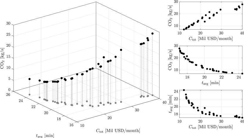
(a) Left: Three-dimensional representation of antichain elements and their projection in the cost-time space. Right: Two-dimensional projections.

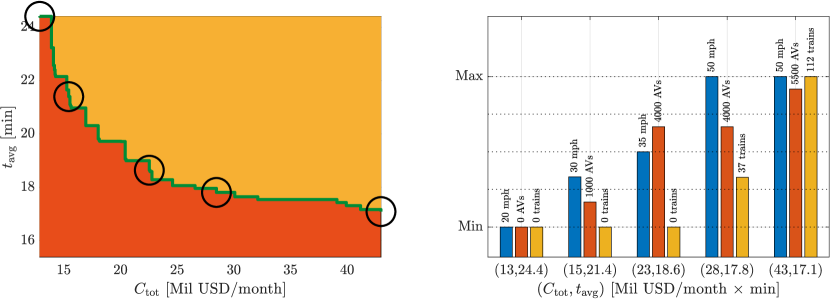
(b) Results for constant automation costs. On the left, the two-dimensional representation of the antichain elements: In red are the unfeasible strategies, in orange the feasible but irrational solutions, and in green the Pareto front. On the right, the implementations corresponding to the highlighted antichain elements, quantified in terms of achievable vehicle speed, AV fleet size, and train fleet size.

Figure 3: Solution of the CDPI: state-of-the art case.

For the sake of clarity, we opt for a two-dimensional antichain representation, by translating and including the emissions in the total cost. To do so, we consider the conversion factor 40 $\nicefrac{{USD}}{{kg}}$ [45]. Note that since this transformation preserves the monotonicity of the CDPI it smoothly integrates in our framework. Doing so, we can conveniently depict the co-design strategies through the two-dimensional antichain (Figure 3(b), left) and the corresponding municipality actions (Figure 3(b), right). Generally, as the municipality budget increases, the average travel time per trip required to satisfy the given demand decreases, reaching a minimum of about 17.1 min with an expense of around 43 $\nicefrac{{MilUSD}}{{month}}$. This configuration corresponds to a fleet of 5,500 AVs able to drive at 50 mph and to the doubling of the current MetroRail train fleet. On the other hand, the smallest rational investment of 12.9 $\nicefrac{{MilUSD}}{{month}}$ leads to a 42 % higher average travel time, corresponding to a inexistent autonomous fleet and an unchanged subway infrastructure. Notably, an expense of 23 $\nicefrac{{MilUSD}}{{month}}$ (48 % lower than the highest rational investment) only increases the minimal required travel time by 9 %, requiring a fleet of 4,000 vehicles able to drive at 35 mph and no acquisition of trains. Conversely, an investment of 15.6 $\nicefrac{{MilUSD}}{{month}}$ (just 2 $\nicefrac{{MilUSD}}{{month}}$ more than the minimal rational investment) provides a 3 min shorter travel time. Remarkably, the design of AVs able to exceed 40 mph only improves the average travel time by 6 %, and it is rational just starting from an expense of 22.8 $\nicefrac{{MilUSD}}{{month}}$. This suggests that the design of faster vehicles mainly results in higher emission rates and costs, without substantially contributing to a more time-efficient demand satisfaction. Finally, it is rational to improve the subway system only starting from a budget of 28.5 $\nicefrac{{MilUSD}}{{month}}$, leading to a travel time improvement of just 4 %. This trend can be explained with the high train acquisition and increased operation costs, related to the subway reinforcement. We expect this phenomenon to be more marked for other cities, considering the moderate operation costs of the MetroRail subway system due to its automation [44] and related benefits [46].

IV-C Case 2 - Speed-Dependent Automation Costs

To relax the potentially unrealistic assumption of a velocity-independent automation cost, we consider a performance-dependent cost structure. The large variance in sensing technologies and their reported performances [47] suggests that this rationale is reasonable. Indeed, the technology required today to safely operate an autonomous vehicle at 50 mph is substantially more sophisticated, and therefore more expensive, than the one needed at 20 mph. To this end, we adopt the cost structure reported in Table I. Furthermore, the frenetic evolution of automation techniques intricates their monetary quantification. Therefore, we perform our studies with current (2020) costs as well as with their projections for the upcoming decade (2025) [48, 34].

IV-C1 Case 2.1 - 2020

We study the hypothetical case of an immediate AV fleet deployment. We introduce the aforementioned velocity-dependent automation cost structure and obtain the results reported in Figure 4(a). Comparing these results with the state-of-the-art parameters presented in Figure 3 confirms the previously observed trend concerning high vehicle speeds. Indeed, spending 24.9 $\nicefrac{{MilUSD}}{{month}}$ (55 % lower than the highest rational expense) only increases the average travel time by 10 %, requiring a fleet of 3,000 AVs at 40 mph and no subway interventions. Nevertheless, the comparison shows two substantial differences. First, the budget required to reach the minimum travel time of 17.1 min is 28 % higher compared to the previous case, and consists of the same strategy for the municipality, i.e., doubling the train fleet and having a fleet of 5,500 AVs at 50 mph. Second, the higher vehicle costs result in an average AV fleet growth of 5 %, an average velocity reduction of 9 %, and an average train fleet growth of 7 %. This trend suggests that, compared to Case 1, rational design strategies foster larger fleets and less performing AVs.

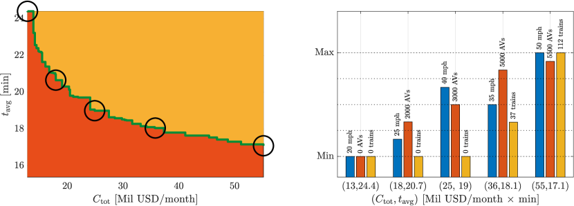
(a) Results for speed-dependent automation costs in 2020.

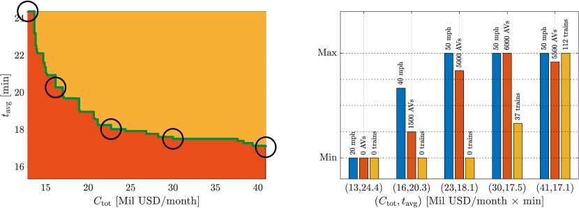
(b) Results for speed-dependent automation costs in 2025.

Figure 4: Results for the speed-dependent automation costs. On the left, the two-dimensional representation of the antichain elements: In red are the unfeasible strategies, in orange the feasible but irrational solutions, and in green the Pareto front. On the right, the implementations corresponding to the highlighted antichain elements.

IV-C2 Case 2.2 - 2025

Experts forecast a substantial decrease of automation costs (up to 90 %) in the next decade, mainly due to mass-production of the AVs sensing technology [48, 49]. In line with this prediction, we inspect the futuristic scenario by solving the CDPI for the adapted automation costs, and report the results in Figure 4(b). Two comments are in order. First, the maximal rational budget is 25 % lower than in the immediate adoption case. Second, the reduction in autonomy costs clearly eases the acquisition of more performant AVs, increasing the average vehicle speed by 10 %. As a direct consequence, the AV and train fleets are reduced in size by 5 % and 10 %, respectively.

IV-D Discussion

We conclude the analysis of our case study with two final comments. First, the presented case studies illustrate the ability of our framework to extract the set of rational design strategies for an AV-enabled mobility system. This way, stakeholders such as AVs companies, transportation authorities, and policy makers can get transparent and interpretable insights on the impact of future interventions. Second, we perform a sensitivity analysis through the variation of the autonomy cost structures. On the one hand, this reveals a clear transition from small fleets of fast AVs (in the case of low autonomy costs) to slow fleets of numerous AVs (in the case of high autonomy costs). On the other hand, our studies highlight that investments in the public transit infrastructure are rational only when large budgets are available. Indeed, the onerous train acquisition and operation costs lead to a comparative advantage of AV-based mobility.

V Conclusion

In this paper, we leveraged the mathematical theory of co-design to propose a design framework for AV-enabled mobility systems. Specifically, the nature of our framework allows both for the modular and compositional interconnection of the DPIs of different mobility options and for multiple objectives. Starting from the multi-commodity flow model of an I-AMoD system, we optimize the design of AVs and public transit both from a vehicle-centric and fleet-level perspective. In particular, we studied the problem of deploying a fleet of AVs providing on-demand mobility in cooperation with public transit, optimizing the speed achievable by the vehicles, the fleet size, and the service frequency of the subway lines. Our framework allows the stakeholders involved in the mobility ecosystem, from vehicle developers all the way to mobility-as-a-service companies and governmental authorities, to characterize rational trajectories for technology and investment development. We showcased our methodology on a real-world case study of Washington D.C., USA. Notably, our problem formulation allows for a systematic analysis of incomparable objectives, providing stakeholders with analytical insights for the socio-technical design of AV-enabled mobility systems. This work opens the field for the following future research streams:
Modeling: First, we would like to extend the presented framework to capture additional modes of transportation, such as micromobility, and heterogeneous fleets with different self-driving infrastructures, propulsion systems, and passenger capacity. Second, we would like to investigate variable demand models. Finally, we would like to analyze the interactions between multiple stakeholders, characterizing the equilibrium arising from their conflicting interests.
Algorithms: It is of interest to tailor co-design algorithmic frameworks to the particular case of transportation DPIs, possibly leveraging their specific structure.
Application: Finally, we would like to devise a user-friendly web interface which supports mobility stakeholders to reason about strategic interventions in urban areas.

References

- [1] G. Zardini, N. Lanzetti, M. Salazar, A. Censi, E. Frazzoli, and M. Pavone, “Towards a co-design framework for future mobility systems,” in Annual Meeting of the Transportation Research Board, Washington D.C., United States, 2020.
- [2] A. Censi, “A mathematical theory of co-design,” arXiv preprint arXiv:1512.08055v7, 2015.
- [3] ——, “Monotone co-design problems; or, everything is the same,” in American Control Conference, 2016.
- [4] ——, “A class of co-design problems with cyclic constraints and their solution,” IEEE Robotics and Automation Letters, vol. 2, pp. 96–103, 2017.
- [5] M. Salazar, N. Lanzetti, F. Rossi, M. Schiffer, and M. Pavone, “Intermodal autonomous mobility-on-demand,” IEEE Transactions on Intelligent Transportation Systems, 2019.
- [6] R. Z. Farahani, E. Miandoabchi, W. Y. Szeto, and H. Rashidi, “A review of urban transportation network design problems,” European Journal of Operational Research, vol. 229, pp. 281–302, 2013.
- [7] V. Guihaire and J.-K. Hao, “Transit network design and scheduling: A global review,” Transportation Research Part B: Methodological, vol. 42, pp. 1251–1273, 2008.
- [8] Z. Cong, B. De Schutter, and R. Babuska, “Co-design of traffic network topology and control measures,” Transportation Research Part C: Emerging Technologies, vol. 54, pp. 56–73, 2015.
- [9] R. O. Arbex and C. B. da Cunha, “Efficient transit network design and frequencies setting multi-objective optimization by alternating objective genetic algorithm,” Transportation Research Part B: Methodological, vol. 81, pp. 355–376, 2015.
- [10] L. Sun, J. G. Jin, D.-H. Lee, K. W. Axhausen, and A. Erath, “Demand-driven timetable design for metro services,” Transportation Research Part C: Emerging Technologies, vol. 46, pp. 284–299, 2014.
- [11] S. Su, X. Li, T. Tang, and Z. Gao, “A subway train timetable optimization approach based on energy-efficient operation strategy,” IEEE Transactions on Intelligent Transportation Systems, vol. 14, no. 2, pp. 883–893, 2013.
- [12] S. Narayanan, E. Chaniotakis, and C. Antoniou, “Shared autonomous vehicle services: A comprehensive review,” Transportation Research Part C: Emerging Technologies, vol. 111, pp. 255–293, 2020.
- [13] J. A. Barrios and J. D. Godier, “Fleet sizing for flexible carsharing systems: Simulation-based approach,” Transportation Research Record: Journal of the Transportation Research Board, vol. 2416, pp. 1–9, 2014.
- [14] D. J. Fagnant and K. M. Kockelman, “Dynamic ride-sharing and fleet sizing for a system of shared autonomous vehicles in austin, texas,” Transportation, vol. 45, no. 1, pp. 143–158, 2018.
- [15] M. M. Vazifeh, P. Santi, G. Resta, S. H. Strogatz, and C. Ratti, “Addressing the minimum fleet problem in on-demand urban mobility,” Nature, vol. 557, no. 7706, p. 534, 2018.
- [16] P. M. Boesch, F. Ciari, and K. W. Axhausen, “Autonomous vehicle fleet sizes required to serve different levels of demand,” Transportation Research Record: Journal of the Transportation Research Board, vol. 2542, no. 1, pp. 111–119, 2016.
- [17] K. Spieser, K. Treleaven, R. Zhang, E. Frazzoli, D. Morton, and M. Pavone, “Toward a systematic approach to the design and evaluation of automated mobility-on-demand systems: A case study in singapore,” in Road vehicle automation, 2014, pp. 229–245.
- [18] H. Zhang, C. J. R. Sheppard, T. Lipman, and S. Moura, “Joint fleet sizing and charging system planning for autonomous electric vehicles,” IEEE Transactions on Intelligent Transportation Systems, 2019.
- [19] G. J. Beaujon and M. A. Turnquist, “A model for fleet sizing and vehicle allocation,” Transportation Science, vol. 25, no. 1, pp. 19–45, 1991.
- [20] A. Wallar, W. Schwarting, J. Alonso-Mora, and D. Rus, “Optimizing multi-class fleet compositions for shared mobility-as-a-service,” in Proc. IEEE Int. Conf. on Intelligent Transportation Systems. IEEE, 2019, pp. 2998–3005.
- [21] H. K. R. F. Pinto, M. F. Hyland, H. S. Mahmassani, and I. O. Verbas, “Joint design of multimodal transit networks and shared autonomous mobility fleets,” Transportation Research Part C: Emerging Technologies, 2019.
- [22] C. F. Daganzo and N. Geroliminis, “An analytical approximation for the macroscopic fundamental diagram of urban traffic,” Transportation Research Part B: Methodological, vol. 42, no. 9, pp. 771–781, 2008.
- [23] PIM. (2012) Metrorail ridership by origin and destination. Plan It Metro. Plan It Metro.
- [24] A. Mas-Colell, M. D. Whinston, and J. R. Green, Microeconomic Theory. Oxford Univ. Press, 1995.
- [25] D. C. Richards, “Relationship between speed and risk of fatal injury: Pedestrians and car occupants,” Department for Transport: London, Tech. Rep., 2010.
- [26] C. Ruch, S. Hörl, and E. Frazzoli, “Amodeus, a simulation-based testbed for autonomous mobility-on-demand systems,” in Proc. IEEE Int. Conf. on Intelligent Transportation Systems, 2018, pp. 3639–3644.
- [27] M. Haklay and P. Weber, “OpenStreetMap: User-generated street maps,” IEEE Pervasive Computing, vol. 7, no. 4, pp. 12–18, 2008.
- [28] GTFS. (2019) Gtfs: Making public transit data universally accessible.
- [29] ODDC. (2017) Taxicab trips in 2016. Open Data DC. Open Data DC. Available online at https://opendata.dc.gov/search?q=taxicabs.
- [30] F. Siddiqui. (2018) As ride hailing booms in d.c., it’s not just eating in the taxi market – it’s increasing vehicle trips. The Washington Post. The Washington Post. available online.
- [31] DoA, Ed., Military Police Traffic Operations. Department of the Army, 1977.
- [32] S. Dixon, H. Irshad, and V. White, “Deloitte city moblity index – washington d.c.” Deloitte, Tech. Rep., 2018.
- [33] A. Censi. (2019) Monotone co-design problems. Available online: https://co-design.science/index.html.
- [34] N. Pavlenko, P. Slowik, and N. Lutsey, “When does electrifying shared mobility make economic sense?” The International Council on Clean Transportation, Tech. Rep., 2019.
- [35] P. M. Boesch, F. Becker, H. Becker, and K. W. Axhausen, “Cost-based analysis of autonomous mobility services,” Transport Policy, vol. 64, pp. 76–91, 2018.
- [36] D. J. Fagnant and K. Kockelman, “Preparing a nation for autonomous vehicles: opportunities, barriers and policy recommendations,” Transportation Research Part A: Policy and Practice, vol. 77, pp. 167–181, 2015.
- [37] G. S. Bauer, J. B. Greenblatt, and B. F. Gerke, “Cost, energy, and environmental impact of automated electric taxi fleets in manhattan,” Environmental Science & Technology, vol. 52, no. 8, pp. 4920–4928, 2018.
- [38] Z. Wadud, “Fully automated vehicles: A cost of ownership analysis to inform early adoption,” Transportation Research Part A: Policy and Practice, vol. 101, pp. 163–176, 2017.
- [39] T. Litman, “Autonomous vehicle implementation predictions – implications for transport planning,” Victoria Transport Policy Institute, Tech. Rep., 2019.
- [40] W. Time. (2018, Mar.) Carbon footprint data. Wired.
- [41] WMATA, “Fy2018 proposed budget,” Washington Metropolitan Area Transit Authority, Tech. Rep., 2017.
- [42] L. Aratani. (2015) Metro to debut first of its 7000-series cars on blue line on april 14. The Washington Post. available online.
- [43] WMATA, “Sustainability report 2018,” Washington Metropolitan Area Transit Authority, Tech. Rep., 2018.
- [44] E. Jaffe. (2015) The case for driverless trains, by the numbers. Citylab. Citylab. Available online.
- [45] P. Howard and D. Sylvan, “Expert consensus on the economics of climate change,” Institute for Policy Integrity – New York University School of Law, Tech. Rep., 2015.
- [46] Y. Wang, J. Zhang, M. Ma, and X. Zhoum, “Survey on driverless train operation for urban rail transit systems,” Urban Rail Transit, vol. 2, no. 3–4, p. 106–113, 2016.
- [47] J. H. Gawron, G. A. Keoleian, R. D. De Kleine, T. J. Wallington, and K. Hyung Chul, “Life cycle assessment of connected and automated vehicles: Sensing and computing subsystem and vehicle level effects,” Environmental Science & Technology, vol. 52, pp. 3249–3256, 2018.
- [48] P. Lienert. (2019) Cost of driverless vehicles to drop dramatically: Delphi ceo. Insurance Journal. available online.
- [49] WCP, “The automotive lidar market,” Woodside Capital Partners, Tech. Rep., 2018.