Massively parallel simulations for disordered systems

Abstract

Simulations of systems with quenched disorder are extremely demanding, suffering from the combined effect of slow relaxation and the need of performing the disorder average. As a consequence, new algorithms, improved implementations, and alternative and even purpose-built hardware are often instrumental for conducting meaningful studies of such systems. The ensuing demands regarding hardware availability and code complexity are substantial and sometimes prohibitive. We demonstrate how with a moderate coding effort leaving the overall structure of the simulation code unaltered as compared to a CPU implementation, very significant speed-ups can be achieved from a parallel code on GPU by mainly exploiting the trivial parallelism of the disorder samples and the near-trivial parallelism of the parallel tempering replicas. A combination of this massively parallel implementation with a careful choice of the temperature protocol for parallel tempering as well as efficient cluster updates allows us to equilibrate comparatively large systems with moderate computational resources.

1 Introduction

Four or five decades of a concerted research effort notwithstanding, systems with strong disorder such as spin glasses and random-field systems Binder and Young (1986); Young (1997) are still puzzling researchers with a fascinating range of rich behaviors that are only partially understood. Examples include the nature of the spin-glass phase in low dimensions Baños et al. (2012); Wang et al. (2014), universality and dimensional reduction at critical points Parisi and Sourlas (1979); Fytas and Martín-Mayor (2013); Fytas et al. (2016), as well as dynamic phenomena such as rejuvenation and aging Baity-Jesi et al. (2018, 2019). While mean-field theory and perturbation expansions for finite dimensions have set the stage for the field Nattermann (1997); Mézard et al. (1987), a lot of the progress in recent years has been through extensive numerical simulations, mostly in the form of Monte Carlo simulations Landau and Binder (2015) and ground-state calculations relying on combinatorial optimization techniques Hartmann and Rieger (2002). While hence computational methods have had a pivotal role in improving our understanding of systems with strong disorder, simulations of such systems are far from technically straightforward. Due to the rugged free-energy landscape Janke (2007) with a multitude of minima separated by energy barriers standard approaches utilizing local updates such as single-spin flip Metropolis or heat-bath algorithms are only able to equilibrate the tiniest of samples, and generalized-ensemble techniques have more recently always been used for simulating spin glasses, in particular, see, e.g., Refs. Berg and Janke (1998); Houdayer (2001); Katzgraber et al. (2006a); Alvarez Baños et al. (2010); Baños et al. (2012); Sharma and Young (2011); Wang et al. (2015a).

Parallel tempering or replica-exchange Monte Carlo has established itself as de facto standard for equilibrium simulations of spin-glass systems Hukushima and Nemoto (1996); Wang et al. (2015b). The main difficulty there relates to the choice of the temperature and sweep protocols for the method in order to achieve optimal (or at least acceptable) mixing behavior of the overall Markov chain. A number of schemes to this end have been proposed in the past Hukushima (1999); Katzgraber et al. (2006b); Bittner et al. (2008); Rozada et al. (2019). The basic methods use fixed temperature sequences following (inversely) linear or exponential progressions, but in many cases these lead to far from optimal performance. Adaptive approaches Hukushima (1999); Katzgraber et al. (2006b); Bittner et al. (2008) move the temperature points and set the sweep numbers in such a way as to dynamically optimize the mixing behavior of the chain, but these typically require rather extensive pre-runs to establish the best parameters. Below we introduce and discuss a compromise approach that uses a family of temperature protocols that can be optimized for the problem studied with moderate effort. It is worthwhile noting that more recently an alternative to parallel tempering known as population annealing Hukushima and Iba (2003); Machta (2010) has gained traction for simulations of disordered systems Wang et al. (2014, 2015a, 2015c); Barash et al. (2019), especially since it is particularly well suited for parallel and GPU computing Barash et al. (2017). In the present paper, however, we focus on the more traditional setup using replica-exchange Monte Carlo.

While parallel tempering has been able to speed up spin-glass simulations dramatically, they still suffer from slow dynamics close to criticality and throughout the ordered phase. Further relief could potentially be expected from approaches alike to the cluster updates that have proven so successful for the simulation of pure or weakly disordered systems Swendsen and Wang (1987); Wolff (1989); Edwards and Sokal (1988); Chayes and Machta (1998). While these methods can be generalized quite easily to the spin-glass case Swendsen and Wang (1986); Liang (1992), the resulting algorithms typically result in clusters that percolate in the high-temperature phase, way above the spin-glass transition, and hence such updates are not efficient Machta et al. (2008). For the case of two dimensions, a cluster method that exchanges clusters between pairs of replicas and thus operates at overall constant energy turns out to be efficient if combined with local spin flips and parallel tempering Houdayer (2001). In three dimensions, however, also this approach is affected by the early percolation problem, although recently a manual reduction of the effective cluster size has been proposed as an ad hoc way of alleviating this problem Zhu et al. (2015). Similar cluster updates have also been discussed for the case of systems without frustrating interactions, but in the presence of random fields Redner et al. (1998).

Even with the best algorithms to hand relaxation times remain daunting, and with the simultaneous presence of strong finite-size corrections to scaling the appetite of researchers studying systems with strong disorder for more computing power seems insatiable. As a result, enormous effort has also been invested in the optimization of implementation details and the utilization of new hardware platforms. One line of research, which is in the tradition of earlier hardware for spin systems Blöte et al. (1999), relates to the design and construction of special-purpose machines based on field-programmable gate arrays (FPGAs) for simulations of spin glasses and related problems Belletti et al. (2009); Baity-Jesi et al. (2014a). While this approach has been very successful Baños et al. (2012); Baity-Jesi et al. (2018, 2019), the financial and time effort invested is enormous, and hence the demand for simpler, off-the-shelf solutions remains strong. A significant competitor in this context are graphics processing units (GPUs) that are able to deliver performances quite comparable to those of the special-purpose machines to a much wider audience of users Weigel (2012). While GPUs are more widely available and easier to program than FPGAs, many of the approaches and code layouts proposed for efficient simulation of spin glasses on GPUs are very elaborate, using a multitude of advanced techniques to speed up the calculation Bernaschi et al. (2011); Yavors’kii and Weigel (2012); Baity-Jesi et al. (2014b); Lulli et al. (2015). In the present paper, instead, we demonstrate how with very moderate effort and a straightforward parallelization of pre-existing CPU code, excellent performance of spin-glass simulations can be achieved on GPU.

The remainder of this paper is organized as follows. In Sec. 2 we introduce the Edwards-Anderson spin glass and the parallel tempering method used for its simulation. Subsequently, we discuss a new parameter-driven scheme for determining an optimized temperature schedule. Finally, we shortly introduce a cluster simulation method originally proposed for simulations of spin glasses in two dimensions. Section 3 discusses the considerations relating to our GPU implementation of this simulation scheme and how it relates to previous spin-glass simulation codes on GPU. In Sec. 4 we benchmark the resulting codes for the Ising spin glass in two and three dimensions, using discrete and continuous coupling distributions. Finally, Sec. 5 contains our conclusions.

2 Model and methods

2.1 Edwards-Anderson spin glass

While methods very similar to those discussed here can be used for simulations of a wide range of lattice spin systems, for the sake of definiteness we focus on the case of the Edwards-Anderson spin-glass model with Hamiltonian Edwards and Anderson (1975)

$$\mathcal{H}=-\sum_{\langle i,j\rangle}J_{ij}s_{i}s_{j}-H\sum_{i}s_{i},$$ (1)

where $s_{i}=\pm 1$ are Ising spins on a $d$-dimensional lattice chosen in the present work to be square or simple cubic, applying periodic boundary conditions. The couplings $J_{ij}$ are quenched random variables which for the examples discussed here are drawn from either a standard normal distribution or from the discrete bimodal,

$$P(J_{ij})=p\delta(J_{ij}-1)+(1-p)\delta(J_{ij}+1).$$ (2)

In zero field, the system undergoes a continuous spin-glass transition in three dimensions Kawashima and Young (1996); Hasenbusch et al. (2008), while there is compelling evidence for a lack of spin-glass order in two-dimensional systems Bhatt and Young (1988).

Two of the basic quantities we consider are the internal energy per spin,

$$e=\frac{1}{N}[\langle\mathcal{H}(\{s_{i}\})\rangle],$$ (3)

where $\langle\cdot\rangle$ denotes a thermal and $[\cdot]$ the disorder average, as well as the Parisi overlap parameter Parisi (1983); Young (1983),

$$q=\left[\left\langle\frac{1}{N}\sum_{i}s_{i}^{(1)}s_{i}^{(2)}\right\rangle\right],$$ (4)

which takes a non-zero value in the spin-glass (but also in a ferromagnetic Berg et al. (2002)) phase. Here, $s_{i}^{(1)}$ and $s_{i}^{(2)}$ denote the spins of two independent systems with the same disorder configuration but different stochastic time evolutions simulated in parallel.

2.2 Parallel tempering simulations

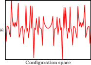
Figure 1: Schematic representation of the rugged energy landscape of a system with strong disorder such as a spin glass.

While for simpler systems single-spin flip simulations using, for instance, the transition probabilities proposed by Metropolis et al. Metropolis et al. (1953) are sufficient to approach stationarity of the Markov chain, this is much more difficult for problems with strong disorder exhibiting a rugged (free) energy landscape as schematically depicted in Fig. 1. At temperatures where the typical energy is below that of the highest barriers, simulations with local, canonical dynamics are not able to explore the full configuration space at reasonable time scales and instead get trapped in certain valleys of the (free) energy landscape. The parallel tempering approach Hukushima and Nemoto (1996) attempts to alleviate this problem by the parallel simulation of a sequence of replicas of the system running at different temperatures. Through equilibrium swap moves of replicas usually proposed for adjacent temperature points, copies that are trapped in one of the metastable states at low temperatures can travel to higher temperatures where ergodicity is restored. Continuing their random walk in temperature space, replicas ultimately wander back and forth between high and low temperatures and thus explore the different valleys of the landscape according to their equilibrium weights. More precisely, the approach involves simulating $N_{T}$ replicas at temperatures $T_{0}<T_{1}<\cdots<T_{N_{T}-1}$. As is easily seen, in order to satisfy detailed balance the proposed swap of two replicas running at temperatures $T_{i}$ and $T_{j}$ should be accepted with probability Hukushima and Nemoto (1996)

$$p_{\mathrm{acc}}=\min\left[1,e^{(1/T_{i}-1/T_{j})(E_{i}-E_{j})}\right],$$ (5)

where $E_{i}$ and $E_{j}$ denote the configurational energies of the two system replicas. If the swap is accepted, replica $i$ will now evolve at temperature $T_{j}$ and replica $j$ at temperature $T_{i}$. On the technical side, it is clear that this can be seen, alternatively, as an exchange of spin configurations or as an exchange of temperatures. While the method does not provide a magic bullet for hard optimization problems where the low lying states are extremely hard to find (such as for“golf course” type of energy landscapes) Machta (2009), it leads to tremendous speed-ups in simulations of spin glasses in the vicinity and below the glass transition, and it has hence established itself as the de facto standard simulational approach for this class of problems.

2.3 Choice of temperature set

The parallel tempering scheme exhibits a number of adjustable parameters which can be tuned to achieve acceptable or even optimal performance. These include, in particular, the temperature set $\{T_{i}\}$ as well as the set $\{\theta_{i}\}$ of the numbers of sweeps of spin flips to be performed at temperature $i$ before attempting a replica exchange move. In the majority of applications $\theta_{i}=\theta$ is chosen independent of the temperature point, and there is some indication that more frequent swap proposals in general lead to better mixing, such that swaps are often proposed after each sweep of spin flips (for some theoretical arguments underpinning this choice see Ref. Dupuis et al. (2012)). Simple schemes for setting the temperature schedule that have been often employed use certain fixed sequences such as an inversely linear temperature schedule, corresponding to constant steps in inverse temperature $\beta$, or a geometric sequence where temperatures increase by a constant factor at each step Predescu et al. (2004); Rozada et al. (2019). For certain problems these work surprisingly well, but there is no good way of knowing a priori whether this will be the case for a given system.

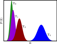
Figure 2: Schematic illustration of the canonical energy histograms at different temperatures. For parallel tempering to work efficiently, all pairs of neighboring temperatures need to have sufficient histogram overlap, such as for the temperatures $T_{0}$, $T_{1}$ and $T_{2}$ shown here. Temperature $T_{3}$, on the other hand, does not provide sufficient overlap with the simulation at $T_{2}$, leading to a poor acceptance rate for the exchange moves.

In order to minimize bias (systematic error) and statistical error, it is clear that the optimal temperature and sweep schedules will result in minimal relaxation times into equilibrium and decorrelation times in equilibrium. As these times are relatively hard to accurately determine numerically Sokal (1997), and they also depend on the observables considered, it is convenient to instead focus on the minimization of the round-trip or tunneling time $\tau_{\mathrm{tunnel}}$, i.e., the expected time it takes for a replica to move from the lowest to the highest temperature and back, which is a convenient proxy for the more general spectrum of decorrelation times. The authors of Ref. Katzgraber et al. (2006b) proposed a method for rather directly minimizing $\tau_{\mathrm{tunnel}}$ by placing temperatures in a way that maximizes the local diffusivity of replicas, but the technique is rather elaborate and the numerical differentiation involved can make it difficult to control. As the random walk of replicas in temperature space immediately depends on the replica exchange events, it is a natural goal to ensure that such swaps occur with a sufficient probability at all temperatures Predescu et al. (2004). It is clear from Eq. (5) that these probabilities correspond to the overlap of the energy histograms at the adjacent temperature points, see also the illustration in Fig. 2. Different approaches have been used to ensure a constant histogram overlap, either by iteratively moving temperature points Hukushima (1999), or by pre-runs and the use of histogram reweighting Bittner et al. (2008). Interestingly, however, constant overlaps do not, in general, lead to minimum tunneling times in cases where the autocorrelation times of the employed microscopic dynamics have a strong temperature dependence, but optimal tunneling can be achieved when using constant overlap together with a sweep schedule taking the temperature dependence of autocorrelation times into account, i.e., by using $\theta_{i}\sim\tau_{\mathrm{can}}(T_{i})$ Bittner et al. (2008).

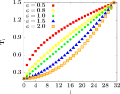
Figure 3: Temperature sequence of the family defined through Eqs. (6) and (7) for $T_{\mathrm{min}}=0.2$ and $T_{\mathrm{max}}=1.5$ with $N_{T}=32$ temperature points and different values of the exponent $\phi$.

While the various optimized schemes lead to significantly improved performance, the additional computational resources required for the optimization are rather substantial, in particular for disordered systems where the optimization needs to be performed separately for each disorder sample. As an alternative we suggest to directly optimize the tunneling times among a suitably chosen family of temperature schedules. The corresponding family of temperature sequences is given by

$$T_{i}=i^{\phi}T_{\rm norm}+T_{\rm min},$$ (6)

where $\phi$ is a free parameter and

$$T_{\rm norm}=\displaystyle\frac{T_{\rm max}-T_{\rm min}}{(N_{T}-1)^{\phi}},$$ (7)

and $N_{T}$ as before denotes the number of temperatures. Clearly, the case $\phi=1$ corresponds to a linear schedule, while $\phi<1$ and $\phi>1$ result in the temperature spacing becoming denser towards higher and lower temperatures, respectively. This is illustrated in Fig. 3, where we show the temperature spacing resulting from different choices of $\phi$ while keeping $T_{\mathrm{min}}$, $T_{\mathrm{max}}$ and $N_{T}$ fixed.

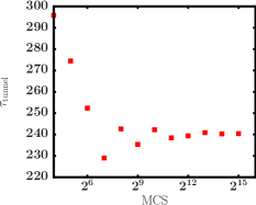
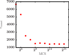
Figure 4: Logarithmically binned time series of tunneling times of parallel tempering simulations of the 2D Gaussian Edwards-Anderson model for individual samples of size $L=15$ (upper panel) and $L=40$ (lower panel), respectively. Here, a Monte Carlo step (MCS) refers to one sweep of spin flips for each replica and one (attempted) replica-exchange move for all replicas.

To optimize the schedule we vary the parameters in the protocol while monitoring the resulting tunneling times. In the following we demonstrate this for the case of the Edwards-Anderson spin glass in two dimensions with Gaussian coupling distribution. We fix $T_{\mathrm{max}}=1.5$, where the system is very quick to relax at any system size and we choose $T_{\mathrm{min}}=0.2$ as the lowest temperature we want to equilibrate the system at. To arrive at reliable estimates for the tunneling times, simulations need to be in equilibrium, and we employ the usual logarithmic binning procedure to ensure this. This is illustrated in Fig. 4 for systems of size $L=15$ and $L=40$, respectively, where it is seen that the tunneling times equilibrate relatively quickly as compared to quantities related to the spin-glass order parameter and so excessively long simulations are not required for the optimization process. Optimizing the protocol then amounts to choosing the exponent $\phi$ and the total number $N_{T}$ of temperature points. To keep the numerical effort at bay we optimize the two parameters separately. The results of the corresponding simulations are summarized in Fig. 5. As the top panel shows, there is a rather clear-cut minimum in the tunneling times as a function of $\phi$ that shifts from $\phi<1$ towards larger values of $\phi$ as the system size $L$ is increased. This trend indicates that for larger systems a higher density of replicas is required at lower temperatures — a tendency that is in line with the general picture of spin-glass behavior.

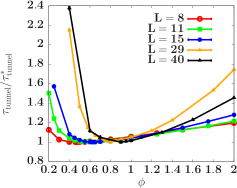
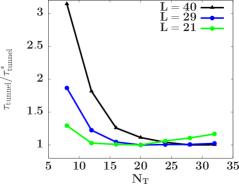
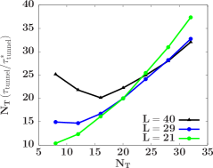
Figure 5: Tunnelling times for parallel tempering simulations with temperature protocol (6) relative to their minimum $\tau_{\mathrm{tunnel}}^{\ast}$ for each system size as a function of the exponent $\phi$ for $N_{T}=32$ (upper panel) and $N_{T}$ for the optimized value $\phi=\phi^{\ast}$ (lower and bottom panels), respectively.

Likewise it is possible to find the optimal number $N_{T}$ of temperature points. The corresponding data from simulations at $\phi=\phi^{\ast}$ for each system size are shown in the middle panel of Fig. 5. It is seen that using too few temperature points leads to rapidly increasing tunneling times. This is a consequence of too small histogram overlaps in this limit. Too many temperature points, on the other, are also found to lead to sub-optimal values of $\tau_{\mathrm{tunnel}}$, which is an effect of the increasing number of temperature steps that need to be traversed to travel from the lowest to the highest temperature (and back) as $N_{T}$ is increased. This effect only sets in for relatively large $N_{T}$, however, and as is seen in the middle panel of Fig. 5 there is a rather shallow minimum for sufficiently large numbers of replicas. To find the optimum investment in computer time, on the other hand, it is useful to also consider the tunneling time in units of (scalar) CPU time, which is expected to be proportional to $N_{T}\tau_{\mathrm{tunnel}}$. This is shown in the bottom panel of Fig. 5, where it becomes clear that the optimal choice in terms of the total computational effort shifts significantly towards smaller $N_{T}$. If copies at different temperatures are simulated in parallel, on the other hand, it is more appropriate to consider the latency instead of the total work, in which case the choice suggested by the middle panel of Fig. 5 is more relevant.

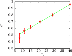
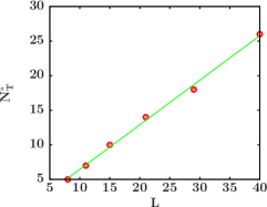
Figure 6: Optimized parameters $\phi^{\ast}$ and $N_{T}^{\ast}$ for parallel tempering simulations of the 2D Gaussian Edwards-Anderson spin glass as a function of linear system size $L$.

Good values for $\phi$ and $N_{T}$ can be inferred for system sizes not directly simulated by applying finite-size scaling. In Fig. 6 we show the optimal values $\phi^{\ast}$ and $N_{T}^{\ast}$ determined from the procedure above as a function of system size $L$. As is seen from the plot, both quantities are approximately linear in $L$, and so we perform fits of the functional form

$$\phi^{\ast}(L)=a_{\phi}+b_{\phi}L$$ (8)

and

$$N_{T}^{\ast}(L)=a_{N_{T}}+b_{N_{T}}L$$ (9)

to the data, resulting in $a_{\phi}=0.406$, $b_{\phi}=0.014$ and $a_{N_{T}}=0.025$, $b_{N_{T}}=0.644$, respectively. We note that on general grounds Janke (2008) we expect that the required number of temperatures $N_{T}$ grows like $L^{d/2}$, and so a steeper than linear increase of $N_{T}$ is expected in three dimensions. The resulting fits are convenient mechanisms for predicting good values for the schedule parameters for larger or intermediate system sizes. We note that both the curves for $\phi$ and $N_{T}$ do not show very sharp minima in $\tau_{\mathrm{tunnel}}$, such that the scheme is not extremely sensitive with respect to the precise choice of parameter values, cf. the results in Fig. 5.

2.4 Cluster updates

Even with the help of parallel tempering it remains hard to equilibrate the spin-glass systems considered here. An additional speed-up of relaxation can come from the use of non-local updates, in particular for the case of systems in two dimensions. An efficient cluster update for this case was first proposed by Houdayer Houdayer (2001). It is similar in spirit to the approach suggested much earlier by Swendsen and Wang Swendsen and Wang (1986), but it uses replicas running at the same temperature. For two such copies with identical coupling configuration $\{J_{ij}\}$ the method operates on the space of the overlap variables,

$$q_{i}=s_{i}^{(1)}s_{i}^{(2)}.$$ (10)

cf. the definition of the total overlap in Eq. (4). To perform an update one randomly chooses a lattice site $i_{0}$ with $q_{i_{0}}=-1$ and iteratively identifies all neighboring spins that also have $q_{i}=-1$, which is most conveniently done using a breadth-first search. The update then consists in exchanging the spin configuration of all lattice sites thus identified to belong to the cluster. As is easily seen, while the energy of both configurations will potentially change, the total energy $E^{(1)}+E^{(2)}$ remains unaltered. Hence such moves can always be accepted and the approach is rejection free. For the same reason it is clearly not ergodic and it hence must be combined with another update such as single-spin flips to result in a valid Markov chain Monte Carlo method. As it turns out, the clusters grown in this way percolate (only) as the critical point $T=0$ of the square-lattice system is approached, and as was demonstrated in Ref. Houdayer (2001) the method hence leads to a significant speed-up of the dynamics.

To implement this technique in practice, we hence use the two replicas of the system at each temperature already introduced in Eq. (4). Following Ref. Houdayer (2001) also larger numbers of replicas at each temperature could be used, but in practice we find little advantage of such a scheme, and it is instead more advisable to invest additionally available computational resources into simulations for additional disorder realisations. We note that with some modifications the same approach might also be used for systems in three and higher dimensions Zhu et al. (2015), although the accelerating effect might be weaker there. In total our updating scheme hence consists of the following steps:

1. Perform $N_{\mathrm{metro}}$ Metropolis sweeps for each replica (usually we choose $N_{\mathrm{metro}}=1$).

2. Perform one Houdayer cluster move for each pair of replicas running with the same disorder and at the same temperature.

3. Perform one parallel tempering update for all pairs of replicas running with the same disorder at neighboring temperatures.

In the following, we will refer to one such full update as a Monte Carlo step (MCS).

The simulation scheme for spin-glass systems described so far is completely generic, and it can be implemented with few modifications on a wide range of different architectures and using different languages. In the following, we will discuss how it can be efficiently realized on GPUs using CUDA.

3 Implementation on GPU

From the description of simulation methods in Sec. 2 it is apparent that a simulation campaign for a system with strong disorder naturally leads to a computational task with manifold opportunities for a parallel implementation: parallel tempering requires to simulate up to a few dozen replicas at different temperatures, the measurement of the overlap parameter $q$ and the cluster update mandate to simulate two copies at each temperature, and finally the disorder average necessitates to consider many thousands of samples. This problem is hence ideally suited for the massively parallel environment provided by GPUs. A number of GPU implementations of spin-glass simulation codes have been discussed previously, see, e.g., Refs. Weigel (2012); Yavors’kii and Weigel (2012); Fang et al. (2014); Baity-Jesi et al. (2014b); Lulli et al. (2015). In the present work we focus on a reasonably simple but still efficient approach that also allows to include an implementation of the cluster updates that have not previously been adapted to GPU (but see Ref. Weigel (2011) for a GPU code for cluster-update simulations of ferromagnets).

Our implementation targets the Nvidia platform using CUDA cud , but a very similar strategy would also be successful for other platforms and OpenCL Scarpino (2012). GPUs offer a hybrid form of parallelism with a number of multiprocessors that each provide vector operations for a large number of leightweight threads. Such threads are organized in a grid of blocks that are independently scheduled for execution Kirk and Hwu (2010); McCool et al. (2012). Of crucial importance for achieving good performance is the efficient use of the memory hierarchy, and in particular the goal of ensuring locality of memory accesses of threads in the same block, as well as the provision of sufficient parallel “slack”, i.e., the availability of many more parallel threads than can actively execute instructions on the given hardware simultaneously Weigel (2018). The latter requirement, which is a consequence of the approach of “latency hiding”, where thread groups waiting for data accesses are set aside in favor of other groups that have completed their loads or stores and can hence continue execution without delays, is easily satisfied in the current setup by ensuring that the total number of replicas simulated simultaneously is sufficiently large.

To achieve the goal of locality in memory accesses, also known as “memory coalescence” in the CUDA framework Kirk and Hwu (2010), it is crucial to tailor the layout of the spin configurations of different replicas in memory to the intended access pattern. In contrast to some of the very advanced implementations presented in Refs. Yavors’kii and Weigel (2012); Fang et al. (2014); Baity-Jesi et al. (2014b); Lulli et al. (2015), here we parallelize only over disorder samples and the replicas for parallel tempering and the cluster update and hence avoid the use of a domain decomposition and additional tricks such as multi-spin coding etc. This leads to much simpler code and, as we shall see below, it still results in quite good performance. Additionally, it has the advantage of being straightforward to generalize to more advanced situations such as systems with continuous spins or with long-range interactions. To facilitate the implementation of the replica-exchange and cluster updates, it is reasonable to schedule the replicas belonging to the same disorder realization together. We hence use CUDA blocks of dimension $(N_{T},N_{C},N_{R})$, where $N_{T}$ is the number of temperatures used in parallel tempering, $N_{C}$ is the number of replicas at the same temperature used in the cluster update, and $N_{R}$ denotes the number of distinct disorder configurations simulated in the same block, cf. Fig. 7 for an illustration. In current CUDA versions, the total number of threads per block cannot exceed $1024$, and the total number of resident threads per multiprocessor cannot exceed $2048$ (or $1024$ for compute capability 7.5). It is usually advantageous to maximize the total number of resident threads per multiprocessor, so a block size of $1024$ threads is often optimal, unless each thread requires many local variables which then suffer from spilling from registers to slower types of memory, but this is not the case of the present problem. To achieve optimal load, it is then convenient to choose $N_{T}$ as a power of two and, given that we always use $N_{C}=2$ (cf. the discussion in Sec. 2.4 above), we then choose $N_{R}=512/N_{T}$. It is of course also possible to use any integer value for $N_{T}$ and then use $N_{R}=\lfloor 512/N_{T}\rfloor$, leading to somewhat sub-optimal performance. Overall, we employ $N_{B}$ blocks, leading to a total of $N_{R}N_{B}$ disorder realizations.

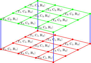
Figure 7: Distribution of threads in a thread block for the spin updates. Each grid point corresponds to a GPU thread, where each thread deals with a copy of the spin system for a different combination of temperature $T_{i}$, replica number $C_{i}$ for cluster updates, and disorder realization $R_{i}$.

In the Metropolis kernel, each thread updates a separate spin configuration, moving sequentially through the lattice. To ensure memory coalescence, the storage for the spin configurations is organized such that the spins on the same lattice site but in different replicas occupy adjacent locations in memory. Note that for each disorder realization $N_{T}N_{C}$ configuration share the sample couplings, such that smaller overall array dimensions are required for accessing the couplings as compared to accessing the spins. Random-site spin updates can also be implemented efficiently in this setup while maintaining memory coalescence by using the same random-number sequence for the site selection but different sequences for the Metropolis criterion (or other update rule) Gross et al. (2018). Random numbers for the updates are generated from a sequence of inline generators local to each thread, here implemented in the form of counter-based Philox generators Salmon et al. (2011); Manssen et al. (2012).

To keep things as simple as possible, the parallel tempering update is performed on CPU Gross et al. (2011). This does not require data transfers as only the configurational energies are required that need to be transferred from GPU to CPU in any case for measurements. The actual spin configurations are not transferred or copied as we only exchange the temperatures. Since even for large-scale simulations no more than a few dozen temperatures are required, this setup does not create a bottleneck for parallel scaling. To implement the bidirectional mapping between temperatures and replicas we use two arrays. On a successful replica exchange move the corresponding entries in the two arrays are swapped. As well shall see below, this leads to very efficient code and the overhead of adding the parallel tempering dynamics on top of the spin flips is quite small.

The cluster update as proposed by Houdayer Houdayer (2001) or any generalizations to higher-dimensional systems Zhu et al. (2015) are implemented in the same general setup, but now a single thread updates two copies as the cluster algorithm operates in overlap space. The block configuration is hence changed to $(N_{T},N_{C}/2,N_{R})$. Given that the register usage is not excessive, this decrease can be compensated by the scheduler by sending twice the number of blocks to each multiprocessor, such that occupancy remains optimal. Due to the irregular nature of the cluster growth, however, full coalescence of memory accesses can no longer be guaranteed, leading to some performance degradation as compared to the spin-flip kernel. A more profound problem results from the fact that the cluster updates discussed in Sec. 2.4 are of the single-cluster nature, such that differences in cluster sizes lead to deviations in run-time between different (pairs of) replicas, such that part of the GPU is idling, thus reducing the computational efficiency. This problem occurs at all levels, from fluctuations between disorder configurations, to different cluster sizes at different temperatures, and even fluctuations in the behavior of different pairs of replicas running with the same disorder and at the same temperature. This is a fundamental limitation of the approach employed here, and we have not been able to eliminate it. Particularly important are the variations with temperature as clusters will be very small at high temperatures and potentially percolating at the lowest temperatures. Possible steps towards alleviating this effect could be to perform several cluster updates in the high-temperature copies while waiting for the low-temperature ones or a formal conversion to a multi-cluster variant which, however, means that all operations on $q=+1$ clusters (i.e., the exchange of spin configurations there) leave the systems invariant. These problems notwithstanding, however, the cluster update if used with moderation where it does not affect the overall parallel efficiency too strongly is still very useful for speeding up the equilibration of the system.

Finally, measurements are taken at certain intervals using the same execution configuration, where measurements of single-replica quantities use blocks of dimensions $(N_{T},N_{C},N_{R})$ and two-replica quantities such as the spin-glass susceptibility and the modes for the correlation length use blocks of size $(N_{T},N_{C}/2,N_{R})$.

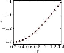
Figure 8: Average internal energy per spin from parallel tempering, cluster update simulations of the 2D Edwards-Anderson spin-glass model with Gaussian couplings implemented on GPU. The data for a linear system size $L=15$ are averaged over 500 disorder samples. The line shows the exact result as calculated by the technique described in Ref. Galluccio et al. (2000).

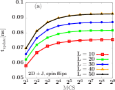
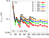
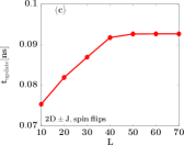
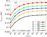
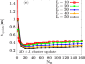
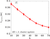
Figure 9: Timing data for simulations of the 2D $\pm J$ Edwards-Anderson model on the Nvidia GTX 1080 GPU. (a)–(c) show the time per spin and update spent in the Metropolis kernel, while (d)–(f) represent the time spent in the cluster-update kernel.

As one step of verification of the correctness of our implementation, we compared the internal energies as a function of temperature found after careful equilibration to the exact result found from a Pfaffian technique that allows to determine the partition function on finite lattices Galluccio et al. (2000). As is apparent from the comparison performed for a sample of $500$ disorder configurations that is shown in Fig. 8 there is excellent agreement, and the simulation data are compatible with the exact result within error bars.

4 Performance

We assess the performance of the GPU implementation discussed above via a range of test runs for the Edwards-Anderson model in two and three dimensions, while using bimodal and Gaussian couplings. For spin-glass simulations, it usually does not make sense to take very frequent measurements of observables as there are strong autocorrelations and the fluctuations induced by the random disorder dominate those that are of thermal origin Picco (1998); Katzgraber et al. (2006a). Hence the overall run-time of our simulations is strongly dominated by the time taken to update the configurations. As is discussed below in Sec. 4.4, the time taken for the parallel tempering moves is small against the time required for spin flips and the cluster update, and it also does not vary between different models, such that we first focus on the times spent in the GPU kernels devoted to the Metropolis and Houdayer cluster updates. To compare different system sizes, we normalize all times to the number of spins in the system, i.e., we consider quantities of the form

$$t_{\mathrm{update}}=\frac{t_{\mathrm{kernel}}}{N_{T}N_{R}N_{C}N_{B}L^{d}},$$ (11)

where $t_{\mathrm{kernel}}$ is the total GPU time spent in a given kernel. The quantity $t_{\mathrm{update}}$ corresponds to the update time per replica and spin for the considered operation. All benchmarks discussed below were performed on an Nvidia GTX 1080, a Pascal generation GPU with 2560 cores distributed over 20 multiprocessors, and equipped with 8 GB of RAM. We expect the general trends observed to be independent of the specific model considered, however.

4.1 Two-dimensional system with bimodal couplings

For the case of a bimodal coupling distribution, $J_{ij}=\pm J$, we store the couplings in 8-bit wide integer variables. For our benchmarks we choose the symmetric case, i.e., $p=1/2$ in Eq. (2). Considering the time spent in the Metropolis and cluster-update kernels separately, we first study how the spin-update times evolve as the systems relax towards equilibrium. In Fig. 9 (a) and (d) we show how the normalized times according to Eq. (11) develop with the number of Monte Carlo steps (MCS) for the Metropolis and cluster-update kernels, respectively. It is clear that for both updates, the run times per step converge relatively quickly, such that after approximately $2^{7}=128$ steps the normalized update times are sufficiently close to stationary. We note that in the present configuration, the normalized times taken for the cluster update are about 2–5 times larger than those for the single-spin flips.

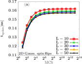
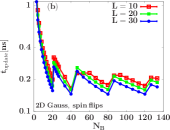
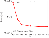
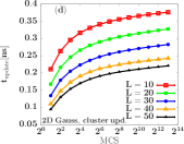
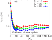
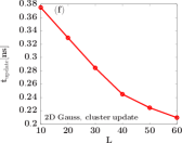
Figure 10: Updating times for GPU simulations of the 2D Gaussian Edwards-Anderson model on the GTX 1080 GPU. Panels (a)–(c) are for the Metropolis kernel, while panels (c)–(f) relate to the cluster update.

As discussed above in Sec. 3, the size of thread blocks should be optimized to result in good performance. Often, best results are achieved for cases of optimal occupancy Weigel (2018), but memory considerations can sometimes shift the corresponding optima. Occupancy plays the key role for the Metropolis kernel as is seen in Fig. 9 (b) which shows $t_{\mathrm{update}}$ as a function of the number $N_{B}$ of thread blocks. As discussed above, $N_{T}$, $N_{C}$ and $N_{R}$ were chosen to result in blocks of $1024$ threads. The limit of $2048$ simultaneously resident threads per multiprocessor means that at most two blocks can be active on each of the $20$ multiprocessors of the GTX 1080 card. As a consequence, the best performance is performed for $N_{B}=40$ and its multiples, with sub-dominant minima at multiples of $N_{B}=20$. For the cluster update this structure is absent, cf. Fig. 9 (e). This is mostly a consequence of the lack of memory coalescence resulting from the cluster algorithm: while in the Metropolis update adjacent threads in a block access adjacent spins in memory, the cluster construction starts from a random lattice site and proceeds in the form of a breadth-first search, resulting in strong thread divergence. Our simulations are hence performed at $N_{B}=40$ which is the dominant minimum for the Metropolis kernel and which is also within the broad minimum for the cluster update.

The lattice-size dependence of GPU performance for the 2D bimodal model is shown in Fig. 9 (c) and (f). As is seen from Fig. 9 (c) the smaller system sizes show slightly smaller spin-flip times than the larger ones. This again is an effect of memory coalescence that is greater for smaller systems where several rows of spins fit into a single cache line. For the cluster update, on the other hand, the decrease of spin-flip times with increasing system size seen in Fig. 9 (f) is an effect of the normalization according to Eq. (11): in each update only a single cluster is grown and the cluster size depends on temperature but only weakly on system size, such that the normalization by $1/L^{2}$ leads to a decay of $t_{\mathrm{update}}$ with $L$.

4.2 Two-dimensional system with Gaussian couplings

Representative of simulations of systems with a continuous coupling distribution we consider the case of Gaussian couplings. The code for this case is very similar to the one for discrete couplings with the difference that now the couplings are stored in $32$-bit floating-point variables. We again run a range of benchmark simulations. The results are summarized in Fig. 10, showing the timings for the Metropolis kernel in panels (a)–(c), and those for the cluster update in panels (d)–(f). Overall, the results are similar to those obtained for the 2D $\pm J$ model, but the updating times are in general somewhat larger for the Gaussian system since the floating-point operations involved in evaluating the Metropolis criterion are more expensive than the integer arithmetic required for the bimodal system. The times for the Metropolis update are almost independent of system size, clearly showing that the increased coalescence that was responsible for higher performance on smaller systems in the bimodal system is no longer relevant here as more time is spent on fetching the couplings and evaluating the acceptance criterion.

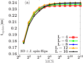
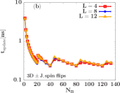
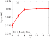
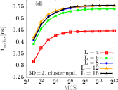
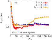
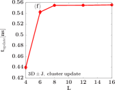
Figure 11: Timing data for GPU simulations of the 3D Edwards-Anderson model with bimodal couplings.

4.3 Three-dimensional system with bimodal couplings

We finally also considered the system with bimodal couplings in three dimensions, where the higher connectivity and related general reduction in memory coalescence leads to an overall increase in spin-flip times in the Metropolis kernel, cf. panels (a)–(c) of Fig. 11. The optimum point of performance at $N_{B}=40$ remains unaltered, and the overall single-spin flip times are very nearly independent of system size, see Fig. 11 (c). The cluster update, on the other hand, appears to be performing very differently from the 2D cases, cf. panels (d)–(f). In particular, we observe that the normalized time spent in the cluster-update kernel does no longer decrease with increasing $L$, but remains constant beyond $L\gtrsim 8$, see panel (f). This is an effect of the cluster algorithm itself, however, and not a shortcoming of the presented implementation: at least without further modifications in the spirit of the proposal put forward in Ref. Zhu et al. (2015) the clusters grown by the construction introduced by Houdayer Houdayer (2001) start to percolate at temperatures significantly above the spin-glass transition point Machta et al. (2008); Zhu et al. (2015). As the times shown in Fig. 11 (f) are effectively an average over the replicas running at all the different temperatures considered, the updating times per spin approach a constant. Here, we do not explicitly attempt to improve the percolation properties of the update itself, but it is clear that our GPU implementation allows such modifications without compromising its performance.

4.4 Cost of the parallel tempering step

As discussed above in Sec. 3, the replica-exchange moves in our code are performed on GPU after transferring the data for the energies from GPU to CPU. While this might seem wasteful, the simplicity of the resulting code appears very attractive if only there is no significant performance penalty associated to this approach. To check whether this is the case we show in Fig. 12 the updating time for the parallel-tempering step for the 2D bimodal system which, according to Eq. (11) is again normalized to a single spin to make the result comparable to the data shown in Figs. 9, 10 and 11. It is clear that for the larger system sizes, where most of the resources for a simulation campaign would be invested, the cost of the replica-exchange steps is small compared to the time spent on updating spins. While the data shown are specifically recorded for simulations of the 2D bimodal Edwards-Anderson model, the time taken for the swap moves only depends on the number of temperature points and it is thus independent of the specific system under consideration, such that the conclusion of negligible cost of the parallel tempering holds even more for the computationally more expensive simulations of the 2D Gaussian and 3D spin-glass models.

4.5 Speed-up

We finally turn to a comparison of the performance of the GPU code introduced above to a reference CPU implementation of exactly the same simulation. The results of this comparison are summarized in Fig. 13. To better understand the performance of different parts of the simulation, we broke the total run-time of both the GPU and CPU simulations into the times spent in (1) flipping spins using the Metropolis algorithm, (2) performing Houdayer’s cluster update, (3) exchanging replicas in the parallel tempering method, and (4) in measurements of the basic observables. The resulting break-down of times is illustrated in the left column of Fig. 13, showing the two-dimensional bimodal (top) and Gaussian (bottom) models, respectively. We find the system size dependence of the times per spin to be rather moderate beyond a certain system size (cf. the representations in Figs. 9 and 10), and consequently we only show results for a single size $L=40$ in Fig. 13. The CPU code was run on a 6-core/12-threads Intel Xeon E5-2620 v3 CPU running at 2.40GHz either using a single thread or running 24 disorder realizations in parallel in the multi-threaded version on a dual-CPU system using hyper-threading, while the GPU code as before was benchmarked on the GTX 1080. It is clearly seen that the CPU code spends the majority of time in flipping spins, whereas on GPU more time is spent in the cluster update as this does not parallelize as well as the Metropolis algorithm. To support this observation further, we show the relative run-times, i.e., speed-ups, of the individual parts of the simulation as compared to the single-threaded (middle column) and multi-threaded (right column) CPU runs, respectively. While we observe speed-ups between GPU and a single CPU thread of between 200 and 300 for the spin flips, the cluster update only improves by a factor of 50–75, on average. The parallel tempering moves, on the other hand, are executed on CPU even in the GPU version of the code and do not experience any speed-up, but their contribution to the overall run-time is negligibly small. Overall, we still observe a speed-up by a factor of about 125 for the whole GPU simulation compared to a single-threaded CPU code. For the multi-threaded CPU implementation run-times are divided by a factor in between the number 12 of physical cores and the number 24 of threads, which indicates good intra-CPU scaling. As a result, compared to a full dual-CPU node our GPU implementation achieves an about eight-fold speed-up overall.

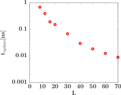
Figure 12: Time spent in the parallel-tempering moves for GPU simulations of the 2D bimodal spin-glass model, normalized to the individual spin. The data are averaged over 640 disorder realizations.

5 Summary

We have discussed the computational challenges of simulating disordered systems on modern hardware, and presented a versatile and efficient implementation of the full spin-glass simulation stack consisting of single-spin flips, cluster updates and parallel-tempering updates in CUDA. Due to the favorable relation of performance to price and power consumption in GPUs, they have turned into a natural computational platform for the simulation of disordered systems. While a range of very efficient, but also very complex, simulational codes for the problem have been proposed before Bernaschi et al. (2011); Yavors’kii and Weigel (2012); Baity-Jesi et al. (2014b); Lulli et al. (2015), our focus in the present work was on the provision of a basic simulation framework that nevertheless achieves a significant fraction of the peak performance of GPU devices for the simulation of spin-glass systems. To be representative of typical installations accessible to users, we used Nvidia GPUs from the consumer series (GTX 1080).

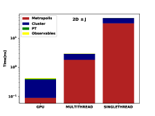
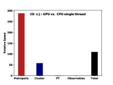
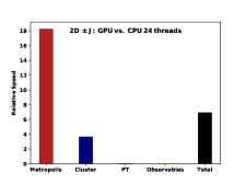
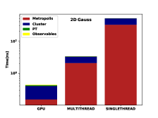
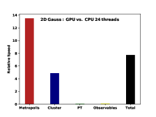
Figure 13: Times spent in different parts of the simulation on a log-scale as compared between the GPU and single-threaded as well as multi-threaded CPU implementations for 2D systems of linear size $L=40$ drawn from bimodal and Gaussian coupling distributions, respectively (left column). The middle and right columns show relative timings (speed-ups) of the GPU code as compared to the single-threaded (middle column) and multi-threaded (right column) CPU runs, respectively.

Comparing our GPU implementation to our reference CPU code, we find a speed-up factor of more than 200 for the Metropolis kernel, which is not far from the performance of more advanced recent GPU simulations of spin models, see, e.g., Ref. Barash et al. (2017). The cluster update algorithm used here is much less well suited for a parallel implementation, especially since it is a single-cluster variant for which the strong variation in cluster sizes leads to the presence of idling threads. Here, performance could be further improved by moving to a multi-cluster code, in line with the experience for ferromagnets Weigel (2011). Nevertheless, overall we still observe a speed-up of the GPU code of about 125 as compared to a single CPU thread, and of about 8 as compared to a full dual-processor CPU node with 24 threads.

In combination with our simple, parametric scheme for choosing the temperature schedule, the proposed simulation framework provides an accessible and highly performant code base for the simulation of spin-glass systems that can easily be extended to other systems with quenched disorder such as the random-field problem Kumar et al. (2018).