Coexistence Mechanism between eMBB and uRLLC in 5G Wireless Networks

Abstract

uRLLC and eMBB are two influential services of the emerging 5G cellular network. Latency and reliability are major concerns for uRLLC applications, whereas eMBB services claim for the maximum data rates. Owing to the trade-off among latency, reliability and spectral efficiency, sharing of radio resources between eMBB and uRLLC services, heads to a challenging scheduling dilemma. In this paper, we study the co-scheduling problem of eMBB and uRLLC traffic based upon the puncturing technique. Precisely, we formulate an optimization problem aiming to maximize the MEAR of eMBB UEs while fulfilling the provisions of the uRLLC traffic. We decompose the original problem into two sub-problems, namely scheduling problem of eMBB UEs and uRLLC UEs while prevailing objective unchanged. Radio resources are scheduled among the eMBB UEs on a time slot basis, whereas it is handled for uRLLC UEs on a mini-slot basis. Moreover, for resolving the scheduling issue of eMBB UEs, we use PSUM based algorithm, whereas the optimal TM is adopted for solving the same problem of uRLLC UEs. Furthermore, a heuristic algorithm is also provided to solve the first sub-problem with lower complexity. Finally, the significance of the proposed approach over other baseline approaches is established through numerical analysis in terms of the MEAR and fairness scores of the eMBB UEs.

I Introduction

The wireless industries are going through different kinds of emerging applications and services, e.g., high-resolution video streaming, virtual reality (VR), augmented reality (AR), autonomous cars, smart cities and factories, smart grids, remote medical diagnosis, unmanned aerial vehicles (UAV), artificial intelligence (AI) based personal assistants, sensing, metering, monitoring etc, along with the explosive trends of mobile traffic [1]. It is foreseen that the mobile application market will flourish in a CAGR of $29.1\%$ during $2015-2020$ [2]. Energy efficiency, latency, reliability, data rate, etc are distinct for separate applications and services. To handle these diversified requirements, International Telecommunication Union (ITU) has already classified 5G services into uRLLC, mMTC, and eMBB categories[3]. Gigabit per second (Gbps) level data rates are required for eMBB users, whereas connection density and energy efficiency are the major concern for mMTC, and uRLLC traffic focuses on extremely high reliability ($99.999\%$) and remarkably low latency ($0.25\sim 0.30$ ms/packet)[4].

Generally, the lions’ share of wireless traffic is produced by eMBB UEs. uRLLC traffic is naturally infrequent and needs to be addressed spontaneously. The easiest way to settle this matter is to allocate some resources for uRLLC. However, under-utilization of radio resources may emerge from this approach, and generally, effective multiplexing of traffics is required. For efficient multiplexing of eMBB and uRLLC traffics, 3GPP has recommended a superposition/puncturing skeleton [4] and the short-TTI/puncturing approaches [5] in 5G cellular systems. Though the short-TTI mechanism is straightforward for implementation, it degrades spectral efficiency because of the massive overhead in the control channel. On the contrary, the puncturing strategy decreases the above overhead, although it necessitates an adequate mechanism for recognizing and healing the punctured case. Slot ($1$ ms) and mini-slot ($0.125$ ms) are proposed as time units for meeting the latency requirement of uRLLC traffic in the 5G NR. At the outset of a slot, eMBB traffic is scheduled and continues unchanged throughout the slot. If the same physical resources are used, uRLLC traffic is overridden upon the scheduled eMBB transmission.

Currently, much attention has been paid to resource sharing for offering QoS or QoE to the users. Studies [6] and [7] investigate the sharing of an unlicensed spectrum between LTE and WiFi networks, however, the study [8] con sider LTE-A and NB-IoT services for sharing the same resources. Study [9] solves user association and resource allocation problems. The study [9] consider the downlink of fog network to support QoS provisions of the uRLLC and eMBB. Some other studies, however, investigates and/or analyzes the influence of uRLLC traffic on eMBB [10, 11, 12, 13, 14, 15] or presents architecture and/or framework for co-scheduling of eMBB and uRLLC traffic [16, 17, 18, 19]. Moreover, some authors consider eMBB and uRLLC traffic in their coexisting/multiplexing proposals [20, 21, 22, 23, 24, 25, 26, 27] where they apply puncturing technique.

As per our knowledge, concrete mathematical models and solutions, however, are lacking in most of these coexistence mechanisms. Most of the studies mainly focus on analysis, system-level design or framework. Thus, effective coexistence proposals between eMBB and uRLLC traffic are wanting in literature. So, to enable eMBB and uRLLC services in $5$G wireless networks, we propose an effective coexistence mechanism in this paper. Our preliminary work has been published in [24] where we have used a one-sided matching and heuristic algorithm, respectively, for resolving resource allocation problems of eMBB and uRLLC users. The major difference between [24] and current work is the involvement of PSUM and TM for solving similar problems. This paper mainly focuses on the followings:

• First, we formulate an optimization problem for eMBB UEs with some constraints, where the objective is to maximize the minimum expected rate of eMBB UEs over time.

• Second, to solve the optimization problem effectively, we decompose it into two sub-problems: resource scheduling for eMBB UEs, and resource scheduling of uRLLC UEs. PSUM is used to solve the first sub-problem, whereas the TM is employed to solve the second one.

• Third, we redefine the first sub-problem into a minimization problem for each slot and provide an algorithm based upon PSUM to obtain near-optimal solutions.

• Fourth, we redefine the second sub-problem as a minimization problem for each mini-slot within every slot and present the algorithm based upon MCC and MODI methods of the transportation model to find an optimal solution of the second sub-problem.

• Fifth, we also present a cost-effective heuristic algorithm for resolving the first sub-problem.

• Finally, we perform a comprehensive experimental analysis for the proposed scheduling approach and compare the results, MEAR and fairness[41] of the eMBB UEs, with the PS [22], MUPS[26], RS, EDS, and MBS approaches.

The remainder of the paper is systematized as follows. In Section II, we present the literature review. We explain the system model and present the problem formulation in Section III. The proposed solution approach of the above-mentioned problem is addressed in Section IV. In Section V, we provide experimental investigation, discussion, and comparison concerning the proposed solution. Finally, we conclude the paper in Section VI.

II Literature Review

Recently, both industry and academia focus on the study of multiplexing between eMBB traffic and uRLLC traffic on the same physical resources. Information-theoretic arguments-based performance analysis for eMBB and uRLLC traffic has performed in [10]. The authors consider both OMA and NOMA for uplink in C-RAN framework. An insight into the performance trade-offs among the eMBB and uRLLC traffic is explained in [10]. In [11], authors have introduced eMBB influenced minimization problem to protect the uRLLC traffic from the dominant eMBB services. This paper explores their proposal for the mobile front-haul environment. In [12], the authors present an effective solution for multiplexing different traffics on a shared resource. Particularly, they propose an effective radio resource distribution method between the uRLLC and eMBB service classes following trade-offs among the reliability, latency and spectral efficiency. Moreover, they investigate the uRLLC and eMBB performance adopting different conditions.

Table I: List of Abbreviations

Abbreviation	Elaboration
uRLLC	Ultra-reliable Low-latency Communication
eMBB, MBB	Enhanced Mobile Broadband, Mobile Broadband
mMTC	Massive Machine-type Communication
PSUM, SUM	Penalty Successive Upper bound Minimization, Successive Upper bound Minimization
TTI	Transmission Time Interval
NR	New Radio
QoS	Quality-of-Service
QoE	Quality-of-Experience
TM, BTM	Transportation Model, Balanced Transportation Model
MCC	Minimum Cell Cost
MODI	Modified Distribution
PS	Punctured Scheduler
MUPS	Multi-User Preemptive Scheduler
RS	Random Scheduler
EDS	Equally Distributed Scheduler
MBS	Matching Based Scheduler
MEAR	Minimum Expected Achieved Rate
NOMA, OMA	Non-orthogonal Multiple Access, Orthogonal Multiple Access
PRB, RB	Physical Resource Block, Resource Block
MIMO	Multiple-input Multiple-output
SINR	signal-to-interference-noise-ratio
gNB	Next Generation Base Station
CP	Combinatorial Programming
CDF, ECDF	Cumulative Distribution Function, Empirical Cumulative Distribution Function
NWC	Northwest corner
VAM	Vogel’s Approximation Method
MCS	Modulation and Coding Scheme
CVaR	Conditional Value at Risk
CAGR	Cumulative Average Growth Rate
C-RAN	Cloud Radio Access Network

In order to 5G service provisioning (i.e., eMBB, mMTC and uRLLC services), the authors of [13] have studied radio resources slicing mechanism, where the performance of both orthogonal and non-orthogonal are analyzed. They have proposed a communication-theoretic model by considering the heterogeneity of 5G services. They also found that the non-orthogonal slicing is significantly better to perform instead of orthogonal slicing for those 5G service multiplexing. Recently, for 5G NR physical layer challenges and solution mechanisms of uRLLC traffic communications has been presented in [14], where they pay attention to the structure of packet and frame. Additionally, they focus on the improvement of scheduling and reliability mechanism for uRLLC traffic communication such that the coexistence of uRLLC with eMBB is established. In [15], the authors have been analyzed the designing principle of the 5G wireless network by employing low-latency and high-reliability for uRLLC traffic. To do this, they consider varying requirements of uRLLC services such as variation of delay, packet size, and reliability. To an extent, they explore different topology network architecture under the uncertainty.

The authors of [16, 17, 18] present a resilient frame formation for multiplexing the provisions of different users. In [16], the authors jointly MBB and mission-critical communication traffic by engaging dynamic TDD and TTI. In [17], the authors represent tractable multiplexing of MBB, MCC, and mMTC considering dynamic TTI. The authors of [18] present a holistic overview of the agile scheduling for 5G that incorporates multiple users. They envision an E2E QoS architecture to offer improved opportunities for application-layer scheduling functionality that ensures QoE for each user. $M/D/m/m$ queueing model-based system-level design has proposed for fulfilling uRLLC traffic demand in [19], where they exhibit that the static bandwidth partitioning is inefficient for eMBB and uRLLC traffic. Thus, the authors of [19] have illustrated a dynamic mechanism for multiplexing of eMBB and uRLLC traffic and apply this in both frequency and time domain.

The efficient way of network resource sharing for the eMBB and uRLLC is studied in [20] and [21]. A dynamic puncturing mechanism is proposed for uRLLC traffic in [20] within eMBB resources to increase the overall resource utilization in the network. To enhance the performance for decoding of eMBB traffic, a joint signal space diversity and dynamic puncturing schemes have proposed, where they improve the performance of component interleaving as well as rotation modulation. In [21], a joint scheduling problem is formulated for eMBB and uRLLC traffic in the goal of maximizing eMBB users’utility while satisfying stochastic demand for the uRLLC UEs. Specifically, they measure the loss of eMBB users for superposition/puncturing by introducing three models, which include linear, convex and threshold-based schemes. For reducing the queuing delay of the uRLLC traffic, the authors introduce punctured scheduling (PS) in [22]. In case of insufficient radio resource availability, the scheduler promptly overwrites a portion of the eMBB transmission by the uRLLC traffic. The scheduler improves the uRLLC latency performance; however, the performance of the eMBB users are profoundly deteriorated. The authors of [23] and [24] manifest the coexistence technique for enabling 5G wireless services like eMBB and uRLLC based upon a punctured scheme. The authors present an enhanced PS (EPS) scheduler to enable an improved ergodic capacity of the eMBB users in [25]. EPS is capable of recovering the lost information due to puncturing and partially. eMBB users are supposed to be cognizant about the corresponding resource that is being penetrated by uRLLC. Therefore, the victim eMBB users ignore the punctured resources from the erroneous chase condensing HARQ process. The authors of [26] propose a MUPS, where they discretize the trade-off among network system capacity and uRLLC performance. MUPS first tries to match the incoming uRLLC traffic inside an eMBB traffic in a conventional MU-MIMO transmission. MUPS serves the uRLLC traffic instantly by using PS if multi-user (MU) pairing cannot be entertained immediately. Though MUPS shows improved spectral efficiency, it is not feasible for uRLLC latency as MU pairing mostly depends on the rate maximization. Hence, the inter-user interference can further degrade the SINR quality of the uRLLC traffic, which can lead to reliability concerns. The authors of [27] propose a null-space-based preemptive scheduler (NSBPS) for jointly serving uRLLC and eMBB traffic in a densely populated 5G arrangement. The proposed approach ensures on-the-spot scheduling for the sporadic uRLLC traffic, while makes a minimal shock on the overall system outcome. The approach employs the system spatial degrees of freedom (SDoF) for uRLLC traffic for spontaneously providing a noise-free subspace. In [28], the authors present a risk-sensitive approach for allocating RBs to uRLLC traffic in the goal of minimizing the uncertainty of eMBB transmission. Particularly, they launch the Conditional Value at Risk (CVaR) for estimating the uncertainty of eMBB traffic in [28].

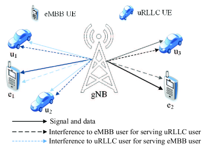
Figure 1: System model for coexisting eMBB and uRLLC services in 5G.

III System Model and Problem Formulation

In this work, we consider a 5G network scenario with one gNB which supports a group of user equipment (UE) $\mathcal{E}$ requiring eMBB service, and a set of user equipment $\mathcal{U}$ demanding uRLLC service. The system operates in downlink mode for the UEs and the overall system diagram is shown in Fig. 1. gNB supports the UEs using licensed RBs $\mathcal{K}$ each with equal bandwidth of $B$. Every time slot, with a length $\Delta$, is split into $M$ mini-slots of duration $\delta$ for managing low latency services. For supporting eMBB UEs, we consider $T_{s}$ LTE time slots and denoted by $\mathcal{T}=\{1,2,\cdots,T_{s}\}$. uRLLC traffic arrive at gNB (any mini-slot $m$ of time slot $t$) follows Gaussian distribution, i.e., $U\sim\mathcal{N}(\mu,\sigma^{2})$. Here, $\mu$ and $\sigma^{2}$ denote the mean and variance of $U$. Each uRLLC UE $u\in\mathcal{U}$ request for a payload of size $L_{u}^{m,t}$ (varying from 32 to 200 Bytes [29]).

Table II: Summary of Notations

Symbol	Meaning
$\mathcal{E}$	Set of active eMBB users
$\mathcal{U}$	Set of uRLLC users
$\mathcal{K}$	Set of RBs of uniform bandwidth $B$
$B$	Bandwidth of a RB
$\Delta$	Duration of a time slot
$\delta$	Duration of a mini-slot
$M$	Number of mini-slots in a time slot
$T$	Total number of time slots
$\lambda$	Mean value of arrival rate of uRLLC traffic
$U$	Random number representing arrival rate of traffics for uRLLC users at mini-slot $m$ of time slot $t$
$L_{u}^{m,t}$	Payload size of uRLLC user $u\in\mathcal{U}$ at mini-slot $m$ of time slot $t$
$\gamma_{e}^{t}$	SNR of eMBB user $e\in\mathcal{E}$ in time slot $t$
$P_{e}$	Transmission power of gNB for eMBB user $e\in\mathcal{E}$
$h_{e}$	Channel gain of for eMBB user $e\in\mathcal{E}$ from gNB
$N_{0}$	Noise spectral density
$\boldsymbol{\alpha}$	Resource allocation vector for $\mathcal{E}$
$\gamma_{u}^{m,t}$	SINR/SNR of uRLLC user $u\in\mathcal{U}$ from gNB at mini-slot $m$ of time slot $t$
$P_{u}$	Transmission power of gNB for uRLLC user $u\in\mathcal{U}$
$h_{u}$	Channel gain of for uRLLC user $u\in\mathcal{U}$ from gNB
$V_{u}$	Channel dispersion for uRLLC user $u$
$N_{u}^{b}$	Blocklength of uRLLC traffic from user $u$
$Q$	Complementary Gaussian cumulative distribution function
$\varepsilon_{u}^{d}$	Probability of decoding error for uRLLC user $u$
$\boldsymbol{\beta}$	Resource allocation vector for $\mathcal{U}$
$\boldsymbol{\phi}$	Vector for representing current serving uRLLC users
$\epsilon$	uRLLC reliability probability
$r_{e,k}^{t}$	Achievable rate of eMBB user $e$ in RB $k$ of time slot $t$
$r_{u,k}^{m,t}$	Achievable rate of uRLLC user $u$ in RB $k$ at mini-slot m of time slot $t$

gNB allots the RBs to the eMBB UEs at the commencement of any time slot $t\in\mathcal{T}$. The achievable rate of $e\in\mathcal{E}$ for RB $k\in\mathcal{K}$ is as follows:

$$\begin{split}r_{e,k}^{t}=\Delta B\log_{2}(1+\gamma_{e,k}^{t}),\end{split}$$ (1)

where $\gamma_{e,k}^{t}=\frac{P_{e}h_{e}^{2}}{N_{0}B}$ presents SNR. $P_{e}$ is the transmission power of gNB for $e\in\mathcal{E}$ and $h_{e}$ denotes the gain of $e\in\mathcal{E}$ from the gNB, and $N_{0}$ represnts the noise spectral density. eMBB UEs require more than one RB for satisfying their QoS. Therefore, the achievable rate of eMBB UE $e\in\mathcal{E}$ in time slot $t$ as follows:

$$\begin{split}r_{e}^{t}=\sum_{k\in\mathcal{K}}\alpha_{e,k}^{t}r_{e,k}^{t},\end{split}$$ (2)

where $\boldsymbol{\alpha}$ denotes the resource allocation vector for $\mathcal{E}$ at any time slot $t$, and each element is as follows:

$$\alpha_{e,k}^{t}=\begin{cases}1,&\text{if RB}\ k\ \text{is allocated for $e\in\mathcal{E}$ at time slot $t$},\\ 0,&\text{otherwise}.\end{cases}$$ (3)

uRLLC traffic can arrive at some moment (i.e. mini-slot) inside any time slot $t$ and requires to be attended quickly. Any uRLLC traffic needs to be completed within a mini-slot period for its’ latency and reliability constraints. Normally, the payload size of uRLLC traffic is really short, and therefore, we cannot straightforwardly adopt Shannon’s data rate formulation[10]. The achievable rate of a uRLLC UE $u\in\mathcal{U}$ in RB $k\in\mathcal{K}$, when its’ traffic is overlapped with eMBB traffic, can properly be approximated by employing [30] as follows:

$$\begin{split}r_{u,k}^{m,t}=\delta\left[B\log_{2}(1+\gamma_{u}^{m,t})-\sqrt{\frac{V_{u}}{N_{u}^{b}}}Q^{-1}(\varepsilon_{u}^{d})\right],\end{split}$$ (4)

where $\gamma_{u}^{m,t}=\frac{h_{u}^{2}P_{u}}{N_{0}B+h_{u}^{2}P_{e}}$ represents the SINR for $u\in\mathcal{U}$ at mini-slot $m$ of $t$. Here, $h_{u}^{2}P_{e}$ indicates the interference generated from serving $e\in\mathcal{E}$ in the same RB, $V_{u}=\frac{h_{u}^{2}P_{u}}{N_{0}B+h_{u}^{2}(P_{u}+P_{e})}$ depicts the channel dispersion, and meaning of other symbols are shown in II. However, the reliability of uRLLC traffic fall into vulnerability due to the interference. Hence, superposition mechanism is not a suitable for serving uRLLC UE[11]. Thus, for serving uRLLC UEs, we concentrate on the puncturing technique . In the punctured mini-slot, gNB allots zero power for eMBB UE, and therefore, the interference cannot affect the uRLLC traffic. At that time, $\gamma_{u}^{m,t}=\frac{h_{u}^{2}P_{u}}{N_{0}B}$ and $V=\frac{h_{u}^{2}P_{u}}{N_{0}B+h_{u}^{2}P_{u}}$. The achieved rate of $u\in\mathcal{U}$, when it uses multiple RBs, is as follows:

$$\begin{split}r_{u}^{m,t}=\sum_{k\in\mathcal{K}}\beta_{e,k}^{m,t}r_{u,k}^{m,t},\end{split}$$ (5)

where $\boldsymbol{\beta}$ is the resource allocation vector for $\mathcal{U}$ at $m$ of $t$, and each of its’ element follows:

$$\beta_{e,k}^{m,t}=\begin{cases}1,&\text{if RB}\ k\ \text{is allocated for $u\in\mathcal{U}$ at $m$ of $t$},\\ 0,&\text{otherwise}.\end{cases}$$ (6)

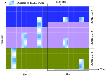
Figure 2: Example of multiplexing between eMBB and uRLLC traffic.

All the uRLLC request in any $m$ of $t$ needs to be served for sure, and hence,

$$\begin{split}P(\sum_{u\in\mathcal{U}}\phi_{u}^{m,t}<U)\leq\epsilon,\forall m,t.\end{split}$$ (7)

where $\boldsymbol{\phi}$ denotes a vector for the serving uRLLC UEs, and thus,

$$\phi_{u}^{m,t}=\begin{cases}1,&\text{if $u\in\mathcal{U}$ is served by the gNB at $m$ of $t$},\\ 0,&\text{otherwise}.\end{cases}$$ (8)

Within the stipulated period $\delta$, the payload $L_{u}^{m,t}$ of $u\in\mathcal{U}$ needs to be transferred, and hence, satisfy the following:

$$\begin{split}\phi_{u}^{m,t}L_{u}^{m,t}\leq\delta r_{u}^{m,t},\forall u,m,t.\end{split}$$ (9)

Hence, the reliability and latency concerns of uRLLC traffic are simultaneously shielded by (7) and (9). Besides, $e\in\mathcal{E}$ loses some throughput at $t$ if uRLLC traffic is punctured within its’ RBs. We utilize the linear model of [21] for estimating the throughput-losses of eMBB UE. Therefore, the throughput-losses $e\in\mathcal{E}$ looks like as follows:

$$\begin{split}r_{e,loss}^{t}=\sum_{k\in\mathcal{K}}r_{e,k}^{t}\sum_{m\in\mathcal{M}}\sum_{u\in\mathcal{U}}\mathbb{I}(\alpha_{e,k}^{t}=\beta_{u,k}^{m,t}).\end{split}$$ (10)

So, the actual achievable rate of $e\in\mathcal{E}$ in any $t$ is as follows:

$$\begin{split}r_{e,actual}^{t}=r_{e}^{t}-r_{e,loss}^{t}.\end{split}$$ (11)

We see that $\boldsymbol{\beta}$ affects on $\boldsymbol{\alpha}$, and hence, impact negatively to the eMBB throughput in each $t\in\mathcal{T}$. At the start of any $t\in\mathcal{T}$, gNB allocates the RBs $\mathcal{K}$ among the $\mathcal{E}$ in an orthogonal fashion as shown in Fig. 2. These characteristics of $\boldsymbol{\alpha}$ are shown mathematically as follows:

$$\begin{split}\sum_{e\in\mathcal{E}}\alpha_{e,k}^{t}&\leq 1,\forall k,\\ \end{split}$$ (12)

$$\begin{split}\sum_{k\in\mathcal{K}}\alpha_{e,k}^{t}&\geq 1,\forall e,\\ \end{split}$$ (13)

$$\begin{split}\sum_{e\in\mathcal{E}}\sum_{k\in\mathcal{K}}\alpha_{e,k}^{t}&\leq|\mathcal{K}|.\\ \end{split}$$ (14)

Within each $t\in\mathcal{T}$, gNB allows uRLLC UEs to get some RBs immediately on a mini-slot basis. Therefore, uRLLC traffic overlaps with eMBB traffic at $m$ and also shown in Fig. 2. Accordingly, $\boldsymbol{\beta}$ satisfy the following conditions on each $m$:

$$\begin{split}\sum_{u\in\mathcal{U}}\beta_{u,k}^{m,t}&\leq 1,\forall k,\end{split}$$ (15)

$$\begin{split}\sum_{k\in\mathcal{K}}\phi_{u}^{m,t}\beta_{u,k}^{m,t}&\geq 1,\forall u,\end{split}$$ (16)

$$\begin{split}\sum_{u\in\mathcal{U}}\sum_{k\in\mathcal{K}}\phi_{u}^{m,t}\beta_{u,k}^{m,t}&\leq|\mathcal{K}|.\end{split}$$ (17)

Finally, our objective is to maximize the actual achievable rate of each eMBB UE across $\mathcal{T}$ while entertaining nearly every uRLLC request within its’ speculated latency. We apply Max-Min fairness doctrine for this mission, and it contributes stationary service quality, enhances spectral efficiency and makes UEs more pleasant in the network. Hence, the maximization problem is formulated as follows:

$$\underset{\boldsymbol{\alpha},\boldsymbol{\beta}}{\max}\ \underset{e\in\mathcal{E}}{\min}\ \mathbb{E}\left(\sum_{t=1}^{|\mathcal{T}|}r_{e,actual}^{t}\right)$$ (18)

s.t. $$P\left(\sum_{u\in\mathcal{U}}\phi_{u}^{m,t}<U\right)\leq\epsilon,\forall m,t,$$ (18a)

$$\phi_{u}^{m,t}L_{u}^{m,t}\leq\delta r_{u}^{m,t},\forall u,m,t,$$ (18b)

$$\sum_{e\in\mathcal{E}}\alpha_{e,k}^{t}\leq 1,\forall k,t,$$ (18c)

$$\sum_{u\in\mathcal{U}}\beta_{u,k}^{m,t}\leq 1,\forall k,m,t,$$ (18d)

$$\sum_{k\in\mathcal{K}}\alpha_{e,k}^{t}\geq 1,\forall e,t,$$ (18e)

$$\sum_{k\in\mathcal{K}}\phi_{u}^{m,t}\beta_{u,k}^{m,t}\geq 1,\forall u,m,t,$$ (18f)

$$\sum_{e\in\mathcal{E}}\sum_{k\in\mathcal{K}}\alpha_{e,k}^{t}+\sum_{u\in\mathcal{U}}\sum_{k\in\mathcal{K}}\phi_{u}^{m,t}\beta_{u,k}^{m,t}\leq|\mathcal{K}|,\forall t,$$ (18g)

$$\alpha_{e,k}^{t},\beta_{u,k}^{m,t},\phi_{u}^{m,t}\in\{0,1\},\forall e,u,k,m,t.$$ (18h)

In (18), the reliability and latency constraints of the uRLLC UEs are preserved by (18a) and (18b). Constraints (18c) and (18d) are used to show the orthogonality of RBs among eMBB and uRLLC UEs, respectively. At least one RB is posed by every active UE and is encapsulated by both (18e) and (18f). Resource restriction is presented by constraint (18g). Constraint (18h) shows that every item of $\boldsymbol{\alpha}$, $\boldsymbol{\beta}$ and $\boldsymbol{\phi}$ are binary. The formulation (18) is a Combinatorial Programming (CP) problem having chance constraint, and NP-hard due to its nature.

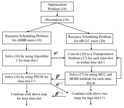
Figure 3: Overview of the Solution Process for (18).

IV Decomposition as a Solution Approach for problem (18)

We assume that eMBB UEs are data-hungry over the considered period. Thus, at the commencement of a time slot $t\in\mathcal{T}$, gNB schedules all of its’ RBs among the eMBB UEs and stay unchanged over $t$. If uRLLC traffic requests come in any $m$ of $t$, the scheduler tries to serve the requests in the next $m+1$. Hence, the overlapping of uRLLC traffic over eMBB traffic happens as shown in Fig. 2. Usually, a portion of all RBs is required for serving such uRLLC traffic. However, the challenge is to find the victimized eMBB UE(s) following the aspiration of the problem (18).

For getting an effective solution to the problem (18), we can utilize the concept of a divide-and-conquer strategy. Here, we divide (18) into two resource allocation sub-problems, namely, for eMBB UEs on time slot basis and uRLLC UEs on a mini-slot basis. The first sub-problem is as follows:

$$\underset{\boldsymbol{\alpha}}{\max}\ \underset{e\in\mathcal{E}}{\min}\ \mathbb{E}\left(\sum_{t=1}^{|\mathcal{T}|}r_{e,actual}^{t}\right)$$ (19)

s.t. $$\sum_{e\in\mathcal{E}}\alpha_{e,k}^{t}\leq 1,\forall k,t,$$ (19a)

$$\sum_{k\in\mathcal{K}}\alpha_{e,k}^{t}\geq 1,\forall e,t,$$ (19b)

$$\sum_{e\in\mathcal{E}}\sum_{k\in\mathcal{K}}\alpha_{e,k}^{t}\leq|\mathcal{K}|,\forall t,$$ (19c)

$$\alpha_{e,k}^{t}\in\{0,1\},\forall e,k,t.$$ (19d)

On the other hand, the second sub-problem (with $\alpha^{t},\forall t$ as the solution of 19) is manifested as follows:

$$\underset{\boldsymbol{\beta}}{\max}\ \underset{e\in\mathcal{E}}{\min}\ \mathbb{E}\left(\sum_{t=1}^{|\mathcal{T}|}r_{e,actual}^{t}\right)$$ (20)

s.t. $$P\left(\sum_{u\in\mathcal{U}}\phi_{u}^{m,t}<U\right)\leq\epsilon,\forall m,t,$$ (20a)

$$\phi_{u}^{m,t}L_{u}^{m,t}\leq\delta r_{u}^{m,t},\forall u,m,t,$$ (20b)

$$\sum_{u\in\mathcal{U}}\beta_{u,k}^{m,t}\leq 1,\forall k,m,t,$$ (20c)

$$\sum_{k\in\mathcal{K}}\phi_{u}^{m,t}\beta_{u,k}^{m,t}\geq 1,\forall u,m,t,$$ (20d)

$$\sum_{u\in\mathcal{U}}\sum_{k\in\mathcal{K}}\phi_{u}^{m,t}\beta_{u,k}^{m,t}\leq|\mathcal{K}|,\forall m,t,$$ (20e)

$$\beta_{u,k}^{m,t},\phi_{u}^{m,t}\in\{0,1\},\forall u,k,m,t.$$ (20f)

Fig. 3 shows the solution overview of the optimization problem (18). We can better understand the philosophy of the problem and the solution approach with an illustrative example in Fig. 2. At the beginning of the time slot, $t-1$, let us assume that there are 3 eMBB UEs, each of whom owns 4 RBs. Within $t-1$, the service request for uRLLC UEs came abruptly and the allocation of RBs for that UEs is shown in Fig. 2, as overlapped uRLLC traffic in the mini-slots. During this time, eMBB users $1,2$ and $3$ waste throughput equivalent to $4$RBs$\times 1$ mini-slot, $7$RBs$\times 1$ mini-slot, and $2$RBs$\times 1$ mini-slot, respectively. At the start of the next time slot, $t$, gNB acknowledges the resource scheduling of uRLLC UEs of $t-1$ to allocate and compensate eMBB UEs. gNB allocates more RBs to eMBB user 2 and less to eMBB user 3 as they lose more and less, respectively, in the time slot $t-1$. Moreover, EgNB tries to serve uRLLC users such that the loss of throughput of eMBB users are almost similar in the time slot $t$. Therefore, gNB makes a balance among the throughput of eMBB users in each time slot, which ultimately serves to reach the goal of (18) on a long-run basis.

IV-A PSUM as a Solution of the Sub-Problem (19)

Problem (19) is still is computationally expensive to reach a globally optimal solution due to its’ NP-hardness. In this sub-section, we propose the PSUM algorithm to solve (19) approximately with low complexity. Relaxation of the binary variable and the addition of a penalty term to the objective function is the main philosophy of our proposed PSUM algorithm. We redefine (19) as follows:

$$\underset{\boldsymbol{\alpha^{t}}}{\min} \sum_{e\in\mathcal{E}}W_{e}^{t}(\boldsymbol{\alpha^{t}}),\forall t,$$ (21)

s.t. $$(\ref{Opt1_1:const1}),(\ref{Opt1_1:const2}),(\ref{Opt1_1:const3}),$$ (21a)

$$W_{e}^{t}(\boldsymbol{\alpha^{t}})=\bigg{|}\frac{1}{t|\mathcal{E}|}\sum_{e^{\prime}\in\mathcal{E}}\bigg{(}\sum_{t^{\prime}=1}^{t-1}r_{e^{\prime},actual}^{t^{\prime}}+r_{e}^{t}\bigg{)}$$

$$\qquad\qquad-\frac{1}{t}\bigg{(}\sum_{t^{\prime}=1}^{t-1}r_{e,actual}^{t^{\prime}}+r_{e}^{t}\bigg{)}\bigg{|},$$ (21b)

$$\alpha_{e,k}^{t}\in[0,1],\forall e,k,t.$$ (21c)

Now according to Theorem 2 of [31], if $|\mathcal{K}|$ is sufficiently large then original sub-problem (19) and (21) are equivalent. Moreover, we add a penalty term $L_{p}$ to the objective function to get binary soltion of relaxed variable from (21). Let $\boldsymbol{\alpha}_{k}^{t}=\{\alpha_{e,k}^{t}\}_{e\in\mathcal{E}}$ and we can rewrite (19a) as $\parallel\boldsymbol{\alpha}_{k}^{t}\parallel_{1}\leq 1,\forall t,k$. The penalized problem is as follows:

$$\underset{\boldsymbol{\alpha^{t}}}{\min} \sum_{e\in\mathcal{E}}W_{e}^{t}(\boldsymbol{\alpha^{t}})+\sigma P_{\varepsilon}(\boldsymbol{\alpha^{t}}),\forall t$$ (22)

s.t. $$(\ref{Opt1_1_2:const3}),(\ref{Opt1_1_2:const4}),(\ref{Opt1_1_2:const5}),$$ (22a)

where $\sigma>0$ is the penalty parameter,

$$\begin{split}P_{\varepsilon}(\boldsymbol{\alpha^{t}})=\sum_{k\in\mathcal{K}}(\parallel\boldsymbol{\alpha}_{k}^{t}+\varepsilon\boldsymbol{1}\parallel_{p}^{p}-c_{\varepsilon,k}).\end{split}$$ (23)

with $p\in(0,1)$, and $\varepsilon$ is any non-negative constant. Following the fact of [32] which is further described in [31], the optimal value is as follows:

$$\begin{split}c_{\varepsilon,k}=(1+\varepsilon)^{p}+(|\mathcal{E}|-1)\varepsilon^{p}.\end{split}$$ (24)

Generally, the parameter $\sigma$ should big enough to make the values of $\{\alpha_{e,k}^{t}\}$ near zero or one. Then, we achieve a feasible solution of (22) by applying the rounding process.

Algorithm 1 Solution of (19) for each $t$ based on PSUM

1:  $\mathbf{Initialization}$: $\varepsilon_{1},\sigma_{1},I_{max}$ and let $i=0$

2:  Solve problem (21) and obtain solution $\boldsymbol{\alpha}^{t,0}$

3:  while $i<I_{max}$ do

4:     Set $\varepsilon=\varepsilon_{i+1}$ and $\sigma=\sigma_{i+1}$

5:     Solve problem (26) with the initial point being $\boldsymbol{\alpha}^{t,i}$, and obtain a new solution $\boldsymbol{\alpha}^{t,i+1}$

6:     if $\boldsymbol{\alpha}^{t,i+1}$ is binary then

7:        Stop

8:     else

9:        Set $i=i+1$

10:        Update $\varepsilon_{i+1}=\eta\varepsilon$, and $\sigma_{i+1}=\zeta\sigma$

11:     end if

12:  end while

It is not easy to solve (22) directly. However, by utilizing the successive upper bound minimization (SUM) technique [33, 34], we can efficiently resolve (22). This method tries to secure the lower bound of the actual objective function by determining a sequence of approximation of the objective functions. As $P_{\varepsilon}(\boldsymbol{\alpha}^{t})$ is concave in nature and hence,

$$\begin{split}P_{\varepsilon}(\boldsymbol{\alpha}^{t})\leq P_{\varepsilon}(\boldsymbol{\alpha}^{t,i})+\nabla P_{\varepsilon}(\boldsymbol{\alpha}^{t,i})^{T}(\boldsymbol{\alpha}^{t}-\boldsymbol{\alpha}^{t,i}),\end{split}$$ (25)

where $\boldsymbol{\alpha}^{t,i}$ is the value of current allocation of iteration $i$. At the $(i+1)$-th iteration of $t$, we solve the following problem:

$$\underset{\boldsymbol{\alpha^{t}}}{\min} \sum_{e\in\mathcal{E}}W_{e}^{t}(\boldsymbol{\alpha^{t}})+\sigma_{i+1}\nabla P_{\varepsilon}(\boldsymbol{\alpha}^{t,i})^{T}\boldsymbol{\alpha^{t}}$$ (26)

s.t. $$(\ref{Opt1_1_2:const3}),(\ref{Opt1_1_2:const4}),(\ref{Opt1_1_2:const5}).$$ (26a)

In each iteration, we can get a globally optimal solution for sub-problem (26) by using the solver. Algorithm 1 shows the proposed mechanism for solving (19). In this Algorithm, $0<\eta<1<\zeta$ where $\zeta$ and $\eta$ represent two constants defined previously.

IV-B Solution of Sub-Problem (20) through TM

Due to the existence of chance constraint (20a) and also the combinatorial variable, $\boldsymbol{\beta}$, (20) is still difficult to resolve by using traditional optimizer. Now, we need to transmute (20a) into deterministic form for solving (20). Moreover, let us assume $g(\boldsymbol{\phi},U)=\sum_{u\in\mathcal{U}}\phi_{u}^{m,t}-U$, $U\in\mathbb{R}$ and $U\sim\mathcal{N}(\mu,\sigma^{2}),\forall m,t$ and hence,

$$Pr\{g(\phi,U)\leq 0\}= Pr\bigg{\{}\sum_{u\in\mathcal{U}}\phi_{u}^{m,t}-U\leq 0\bigg{\}}$$ (27)

$$= Pr\bigg{\{}\sum_{u\in\mathcal{U}}\phi_{u}^{m,t}\leq U\bigg{\}}$$ (27a)

$$= 1-Pr\bigg{\{}\sum_{u\in\mathcal{U}}\phi_{u}^{m,t}\geq U\bigg{\}}$$ (27b)

$$= 1-Pr\bigg{\{}\frac{U-\mu}{\sigma}\leq\frac{\sum_{u\in\mathcal{U}}\phi_{u}^{m,t}-\mu}{\sigma}\bigg{\}}$$ (27c)

$$= 1-F_{U}\left(\sum_{u\in\mathcal{U}}\phi_{u}^{m,t}\right).$$ (27d)

Here, $F_{U}$ is the cumulative distribution function (CDF) of random variable $U$. Thus, from constraint (20a), we can rewrite as follows:

$$Pr\{g(\phi,U)\leq 0\}\geq\epsilon,$$ (28)

$$1-F_{U}\bigg{(}\sum_{u\in\mathcal{U}}\phi_{u}^{m,t}\bigg{)}\leq\epsilon,$$ (28a)

$$F_{U}\bigg{(}\sum_{u\in\mathcal{U}}\phi_{u}^{m,t}\bigg{)}\geq 1-\epsilon,$$ (28b)

$$\sum_{u\in\mathcal{U}}\phi_{u}^{m,t}\geq F_{U}^{-1}\bigg{(}1-\epsilon\bigg{)},$$ (28c)

$$\sum_{u\in\mathcal{U}}\phi_{u}^{m,t}-F_{U}^{-1}(1-\epsilon)\geq 0.$$ (28d)

Now, (28d) and (20a) are identical. Hence, the renewed form of (20) looks like as follows:

$$\underset{\boldsymbol{\beta}^{t}}{\min}\quad \sum_{e\in\mathcal{E}}V_{e}^{t}(\boldsymbol{\alpha^{t}},\boldsymbol{\beta}^{t}),\forall t$$ (29)

s.t. $$\sum_{u\in\mathcal{U}}\phi_{u}^{m,t}-F_{U}^{-1}(1-\epsilon)\geq 0,\forall m,$$ (29a)

$$(\ref{Opt1_2:const2}),(\ref{Opt1_2:const3}),(\ref{Opt1_2:const4}),(\ref{Opt1_2:const5}),(\ref{Opt1_2:const6}),\forall u,m,$$ (29b)

$$V_{e}^{t}(\boldsymbol{\alpha^{t}},\boldsymbol{\beta}^{t})=\bigg{|}\frac{1}{|\mathcal{E}|}\sum_{e^{{}^{\prime}}\in\mathcal{E}}r_{e^{{}^{\prime}},loss}^{t}-r_{e,loss}^{t}\bigg{|},\forall e.$$ (29c)

Problem (29) is still NP-hard due to the appearance of combinatorial variable. In (29), (29a) holds for a particular value of $\epsilon$ when gNB serves a certain portion of uRLLC UE $U^{{}^{\prime}}\leq U$. For a $m$ of $t$, let us assume $\mathcal{U}^{{}^{\prime}}=\{1,2,....,U^{{}^{\prime}}\}$ and $\phi_{u}^{m,t}=1,\forall u\in\mathcal{U}^{{}^{\prime}}$. We can determine the requisite RBs, $\forall u\in\mathcal{U}^{{}^{\prime}}$ holding $\delta$ as the upper-bound in (20b) and let $\boldsymbol{d}=[d_{1},d_{2},\cdots,d_{|\mathcal{U}^{{}^{\prime}}|}]$. As gNB engages OFDMA for uRLLC UEs, constraint (20c) holds. Moreover, depending on $\mathcal{U}^{{}^{\prime}}$, constraints (20d), (20e), and (20f) also hold. Constraint (29c) can be used as a basic block to build a cost matrix $\boldsymbol{C}=(c_{u,e}),u\in\mathcal{U}^{{}^{\prime}},e\in\mathcal{E}$. As $\mathcal{K}$ are held by eMBB UEs $\mathcal{E}$ in any time slot $t\in\mathcal{T}$, we can find a vector $\boldsymbol{s}=[s_{1},s_{2},\cdots,s_{|\mathcal{E}|}]$. Now redefine problem (29) as follows:

$$\underset{\boldsymbol{\chi}}{\min}\quad \sum_{u\in\mathcal{U}^{{}^{\prime}}}\sum_{e\in\mathcal{E}}c_{ue}\chi_{ue}$$ (30)

s.t. $$\sum_{e\in\mathcal{E}}\chi_{ue}=d_{u},\forall u\in\mathcal{U}^{{}^{\prime}},$$ (30a)

$$\sum_{u\in\mathcal{U}^{{}^{\prime}}}\chi_{ue}\leq s_{e},\forall e\in\mathcal{E},$$ (30b)

$$\sum_{u\in\mathcal{U}^{{}^{\prime}}}d_{u}\leq\sum_{e\in\mathcal{E}}s_{e},$$ (30c)

$$\sum_{e\in\mathcal{E}}s_{e}=|\mathcal{K}|,$$ (30d)

$$\chi_{ue}\geq 0,\forall u\in\mathcal{U}^{{}^{\prime}},e\in\mathcal{E}.$$ (30e)

The goal of (30) is to find a matrix $\boldsymbol{\chi}\in\mathbb{Z}^{|\mathcal{U}^{{}^{\prime}}|\times|\mathcal{E}|}=(\chi_{ue}),\forall u\in\mathcal{U}^{{}^{\prime}},e\in\mathcal{E}$ that will minimize the cost/loss of eMBB UEs. This is a linear programming problem equivalent to the Hitchcock problem [35] with inequities, which contributed to unbalanced transportation model. Introducing slack variables $\chi_{|\mathcal{U}^{{}^{\prime}}|+1,e},\forall e\in\mathcal{E}$ and $d_{|\mathcal{U}^{{}^{\prime}}|+1}$ in the constraints (30b) and (30c), respectively, which convert them into equality, we have:

$$\begin{split}\sum_{u\in\mathcal{U}^{{}^{\prime}}}\chi_{ue}+\chi_{|\mathcal{U}^{{}^{\prime}}|+1,e}=s_{e},\forall e\in\mathcal{E},\end{split}$$ (31)

$$\begin{split}\sum_{u\in\mathcal{U}^{{}^{\prime}}}d_{u}+d_{|\mathcal{U}^{{}^{\prime}}|+1}=\sum_{e\in\mathcal{E}}s_{e}.\end{split}$$ (32)

Now the modified problem in (30) is a BTM. Moreover, we have to add $d_{|\mathcal{U}^{{}^{\prime}}|+1}=\sum_{e\in\mathcal{E}}s_{e}-\sum_{u\in\mathcal{U}^{{}^{\prime}}}d_{u}$ to the demand vector $\boldsymbol{d}$ as $\boldsymbol{d}=\boldsymbol{d}\cup\{d_{|\mathcal{U}^{{}^{\prime}}|+1}\}$ and a row $[0]_{1\times|\mathcal{E}|}$ to cost matrix $\boldsymbol{C}$ as $\boldsymbol{C}=\boldsymbol{C}\cup\{[0]_{1\times|\mathcal{E}|}\}$. BTM can be solved by the simplex method [36]. The solution matrix $\boldsymbol{\chi}$ will be in the form of $\mathbb{Z}^{(|\mathcal{U}^{{}^{\prime}}|+1)\times|\mathcal{E}|}$. NWC[37], MCC[37], and VAM[37, 38] are some of the popular methods for obtaining initial feasible solution of BTM. We can use the stepping-stone [39] or MODI [40] method to get an optimal solution of the BTM. In the following sub-section, we use the combination of the MCC and MODI for acquaring the optimal result from the BTM.

IV-B1 Determining Initial Feasible Solution by MCC Method

MCC method allots to those cells of $\boldsymbol{\chi}$ considering the lowest cost from $\boldsymbol{C}$. Firstly, the method allows the maximum permissible to the cell with the lowest per RB cost. Secondly, the amount of quantity and need is synthesized while crossing out the satisfied row(s) or column(s). Either row or column is ruled out if both of them are satisfied concurrently. Thirdly, we inquire into the uncrossed-out cells which have the least unit cost and continue it till there is specifically one row or column is left uncrossed. The primary steps of the MCC method are compiled as follows:

• Step 1: Distribute maximum permissible to the worthwhile cell of $\boldsymbol{\chi}$ which have the minimum cost found from $\boldsymbol{C}$, and update the supply ($\boldsymbol{s}$) and demand ($\boldsymbol{d}$).

• Step 2: Continue Step 1 till there is any demand that needs to be satisfied.

IV-B2 MODI Method for Finding an Optimal Solution

The initial solution found from section IV-B1 is used as input in the MODI method for finding an optimal solution. We need to augment an extra left-hand column and the top row (indicated by $x_{u}$ and $y_{e}$ respectively) with $\boldsymbol{C}$ whose values require to be calculated. The values are measured for all cells which have the corresponding allocation in $\boldsymbol{\chi}$ and shown as follows:

$$\begin{split}x_{u}+y_{e}=c_{u,e},\forall\chi_{u,e}\neq\emptyset.\end{split}$$ (33)

Now we solve (33) to obtain all $x_{u}$ and $y_{e}$. If necessary then assign zero to one of the unknowns toward finding the solution. Next, evaluate for all the empty cells of $\boldsymbol{\chi}$ as follows:

$$\begin{split}k_{u,e}=c_{u,e}-x_{u}-y_{e},\forall\chi_{u,e}=\emptyset.\end{split}$$ (34)

Now select $k_{u,e}$ corresponding to the most negative value and determine the stepping-stone path for that cell to know the reallocation amount to the cell. Next, allocate the maximum permissible to the empty cell of $\boldsymbol{\chi}$ corresponding to the selected $k_{u,e}$. $x_{u}$ and $y_{e}$ values for $\boldsymbol{C}$ and $\boldsymbol{\chi}$ must be recomputed with the help of (33) and a cost change for the empty cells of $\boldsymbol{\chi}$ need to be figured out using (34). A corresponding reallocation takes place just like the previous step and the process continues till there is a negative $k_{u,e}$. At the end of this repetitive process, we get the optimal allocation ($\boldsymbol{\chi}$). The MODI method described above can be summed as follows:

• Step 1: Develop a preliminary solution ($\boldsymbol{\chi}$) applying the MCC method.

• Step 2: For every row and column of $\boldsymbol{C}$, measure $x_{u}$ and $y_{e}$ by applying (33) to each cell of $\boldsymbol{\chi}$ that has an allocation.

• Step 3: For every corresponding empty cell of $\boldsymbol{\chi}$, calculate $k_{u,e}$ by applying (34).

• Step 4: Determine the stepping-stone path [39] from $\boldsymbol{\chi}$ corresponding to minimum $k_{u,e}$ that found in Step 3.

• Step 5: Based on the stepping-stone path found in Step 4, allocate the highest possible to the free cell of $\boldsymbol{\chi}$.

• Step 6: Reiterate Step 2 to 5 until all $k_{u,e}\geq 0$.

IV-C Low-Complexity Heuristic Algorithm for Solving Sub-Problem (19)

Though Algorithm 1 can solve the sub-problem (19) optimally, but computation time requires to solve it grows much faster as the size of the problem increase. Besides, the number of eMBB UEs is large in reality, and we have a short period to resolve this kind of problem. Therefore, we need a faster and efficient heuristic algorithm, which may sacrifice optimality, to solve (19). Thus, we propose Algorithm 2 for solving (19). At $t=1$, Algorithm 2 allocate resources equally to the eMBB UEs. But, it allocates resources to eMBB UEs in the rest of the time slots depending on the proportional loss of the previous time slot. In this way, Algorithm 2 can accommodate the EAR of eMBB UEs in the long-run. The complexity of Algorithm 2 depends on $\mathcal{T}$ and $\mathcal{E}$.

Algorithm 2 Heuristic Algorithm for Solving (19)

1:  $\mathbf{Initialization}$: $\varepsilon_{1},\sigma_{1},I_{max}$ and let $i=0$

2:  Solve problem (21) and obtain solution $\boldsymbol{\alpha}^{t,0}$

3:  for each $t\in\mathcal{T}$ do

4:     if t =1 then

5:        Calculate $N_{RB}=\frac{|\mathcal{K}|}{|\mathcal{E}|}$

6:        for each $e\in\mathcal{E}$ do

7:           for each $k=1\cdots N_{RB}$ do

8:              $\alpha_{e,(e-1)*N_{RB}+k}^{t}=1$

9:           end for

10:        end for

11:     else

12:        Determine $r_{e,loss}^{t-1}$ and $r_{e,actual}^{t-1}$ for all $e\in\mathcal{E}$ by using (10) and (11) respectively

13:        Set $loc=0$

14:        for each $e\in\mathcal{E}$ do

15:           Calculate $N_{RB}^{e}=\frac{r_{e,loss}^{t-1}}{\sum_{e^{\prime}\in\mathcal{E}}r_{e^{\prime},loss}^{t-1}}|\mathcal{K}|$

16:           for each $k=1\cdots N_{RB}^{e}$ do

17:              $\alpha_{e,loc+k}^{t}=1$

18:           end for

19:           Set $loc=loc+N_{RB}^{t}$

20:        end for

21:     end if

22:  end for

23:  Determine $r_{e,actual}^{t}$ for all $e\in\mathcal{E}$ by using (11)

24:  Determine $\mathbb{E}\bigg{(}\sum_{t=1}^{|\mathcal{T}|}r_{e,actual}^{t}\bigg{)}$ for all $e\in\mathcal{E}$

V Numerical Analysis and Discussions

In this section, we assess the proposed approach using comprehensive experimental analyses. Here, we compare our results with the results of the following state-of-the-art schedulers:

• PS[22]: PS immediately overwrite part of the continuing eMBB transmission with the sporadic uRLLC traffic if there are not sufficient PRBs available. It chooses PRBs with the highest MCS that already been allotted to eMBB UEs.

• MUPS[26]: In case of insufficient RBs, MUPS allocates PRBs to the uRLLC UEs where they endure better channel quality depending on the CQI feedback.

• RS: RS takes the RBs from the eMBB UEs randomly in case of inadequate PRBs for supporting uRLLC traffic.

• EDS: For supporting sporadic uRLLC traffic, EDS offers the PRBs to this traffic after preempting PRBs equally from the eMBB UEs in case of unavailable PRBs.

• MBS: gNB uses many to one matching game for snatching PRBs from eMBB UEs for supporting uRLLC traffic.

The main performance parameters are MEAR and fairness [41] of the eMBB UEs and defined as follows:

$$\begin{split}\mbox{MEAR}=\min\ \mathbb{E}\left(\sum_{t=1}^{|\mathcal{T}|}r_{e,actual}^{t}\right),\forall e\in\mathcal{E},\end{split}$$ (35)

$$\begin{split}\mbox{Fairness}=&\frac{\left(\sum_{e\in\mathcal{E}}\mathbb{E}\left(\sum_{t=1}^{|\mathcal{T}|}r_{e,actual}^{t}\right)\right)^{2}}{|\mathcal{E}|\cdot\sum_{e\in\mathcal{E}}\left(\sum_{t=1}^{|\mathcal{T}|}r_{e,actual}^{t}\right)^{2}}.\end{split}$$ (36)

In our scenario, we consider an area with a radius of $200$ m and gNB resides in the middle of the considered area. eMBB and uRLLC UEs are disseminated randomly in the coverage space. gNB works on a $10$ MHz licensed band for supporting the UEs in downlink mode. Every uRLLC UE needs a single PRB for its service. Furthermore, gNB estimates path-loss for both eMBB and uRLLC UEs using a free space propagation model amidst Rayleigh fading. Table III exhibits the significant parameters for this experiment. We use similar PSUM parameters as of [31]. We realize the results of every approaches after taking $1,000$ runs.

Table III: Summary of the simulation setup

Symbol	Value	Symbol	Value
$|\mathcal{E}|$	$10$	$|\mathcal{K}|$	$50$
$B$	$180$ kHz	$\epsilon$	$0.01$
$|\mathcal{T}|$	$1000$	$M$	$8$
$\Delta$	$1$ms	$\delta$	$0.125$ ms
$P_{e},\forall e$	$21$ dBm	$P_{u},\forall u$	$21$ dBm
$I_{max}$	$20$	$N_{0}$	$-114$ dBm
$\sigma$	$1,2,\cdots,10$
$L$	$32,50,100,150,200$ bytes
eMBB traffic model	Full buffer
$\sigma_{1}$	$2$	$\epsilon_{1}$	$0.001$
$\eta$	$0.7$	$\zeta$	$1.1$

A comparison of MEAR and fairness scores are presented in Fig. 4 and Fig. 5, respectively, between the proposed (PSUM+TM) and the optimal value for a small network. Fig. 4 shows the ECDF of MEAR and the probability of MEAR being at least $20$ Mbps are around $0.50$ and $0.70$, respectively, for the proposed and optimal methods, consequently. The optimality gap of average MEAR for the proposed method is $4.20\%$ as represented in Fig. 4. Fig. 5 shows the ECDF of the fairness scores where the probability of the scores being $0.995$ at least is $0.80$ in the proposed method in comparison of being $1$ in the optimal mechanism. The optimality gap of the proposed method for the average fairness score is $0.32\%$ as exposed from Fig. 5.

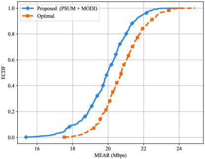
Figure 4: Comparison of MEAR during $\mathcal{E}=4$ and single uRLLC UE in every mini-slot when $L=32$ bytes.

For growing uRLLC arrivals, the ECDF of the MEAR values is exhibited in Fig. 6. Fig. 6 reveals the results that are preferred to those of the other considered methods. The probability of MEAR values for being at least $18.0$ Mbps are $0.889$, $0.405$, $0.367$, $0.653$, $0.653$, and $0.052$ for the proposed, RS, EDS, MBS, PS, and MUPS methods, respectively, that are shown in Fig. 6(a). Fig. 6(b) reveals that the likelihood of MEAR values for obtaining a minimum of $18.0$ Mbps are $0.736$, $0.089$, $0.050$, $0.541$, and $0.647$ for the proposed, RS, EDS, MBS, and PS methods, respectively, while the MUPS method can accommodate under $18$ Mbps in every case. Fig. 6(c) shows that the proposed, MBS and PS methods provide a minimum MEAR value of $18.0$ Mbps with a probability $0.231$, $0.089$, and $0.231$, respectively, while RS, EDS, and MUPS can produce less than $18$ Mbps for sure. Moreover, the MEAR value decreases with the growing rate of $\sigma$ for all the methods because of the requirement of more RBs for the uRLLC UEs as shown in Fig. 6. But, the increasing arrivals of uRLLC traffic affect the MUPS method more as they require extra RBs from the distant eMBB UEs. However, the performance gap between the proposed and PS method reduces with the increased arrival of uRLLC traffic, as the PS scheme gets more chance to adjust the users with the higher expected achieved rate.

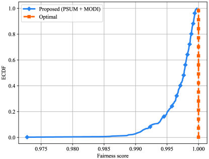
Figure 5: Comparison of fairness score when $\mathcal{E}=4$ and single uRLLC UE in each mini-slot along with $L=32$ bytes.

We compare the fairness scores among various methods with different values of $\sigma$ which is shown in Fig. 7. The scores originating from the proposed method are greater than or similar to that of others as indicated in Fig. 7. Fig. 7(a) reveals that the median of the scores for the proposed, RS, EDS, MBS, PS, and MUPS methods are $0.9977$, $0.9897$, $0.9897$, $0.9975$, $0.9972$, and $0.9789$, respectively. The similar scores are $0.9998$, $0.9902$, $0.9902$, $0.9987$, $0.9995$, $0.9488$, and $1.00$, $0.9891$, $0.9891$, $0.9985$, $0.9998$, $0.8784$ for the corresponding methods and are presented in Fig. 7(b) and 7(c), respectively. Moreover, the fairness scores increase for the Proposed, MBS and PS methods with the increasing value of $\sigma$ as it gets more chance to maximize the minimum achieved rate, whereas the same scores decrease with the increasing value of $\sigma$ for RS, EDS and MUPS as eMBB UEs have more opportunity to be affected by the uRLLC UEs.

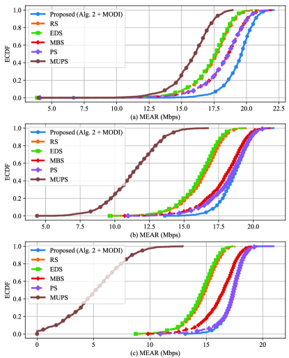
Figure 6: Comparison of MEAR for (a) $\sigma=1$, (b) $\sigma=5$, and (c) $\sigma=10$, along with $L=32$ Bytes.

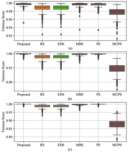
Figure 7: Comparison of fairness scores (a) $\sigma=1$, (b) $\sigma=5$, and (c) $\sigma=10$, along with $L=32$ Bytes.

Fig. 8 and 9, respectively, show the average MEAR and fairness score for varying value of $\sigma$. In Fig. 8, we find that our method overpasses other schemes for different rates of $\sigma$ in the case of average MEAR. The figure also explicates that the average MEAR is declining with the growing value of $\sigma$ due to the additional requirement of PRBs for extra uRLLC traffic. Particularly, our method results $10.20\%$, $10.87\%$, $5.77\%$, $5.77\%$, and $18.55\%$ higher on average MEAR than those of RS, EDS, MBS, PS, and MUPS, respectively, for $\sigma=1$. Moreover, similar values are $15.22\%$, $16.43\%$, $6.22\%$, $3.75\%$, and $70.20\%$ for $\sigma=10$. The average fairness score emerging from our method is bigger than or similar to other comparing methods for different values of $\sigma$ and shown in Fig. 9. Fig. 9 also reveals that the $\sigma$ value has a negligible impact on the average score of the fairness in the Proposed, RS, EDS, MBS, PS methods, but it impacts inversely to the MUPS method more and more uRLLC traffic choose same eMBB UE for the PRBs. Moreover, the average fairness scores of the proposed method are similar to both MBS and PS methods. However, the proposed method treats eMBB UEs $0.92\%$, $0.92\%$, and $1.92\%$ fairly than RS, EDS, and MUPS methods , respectively, when $\sigma=1$, whereas, the similar scores are $1.23\%$, $1.23\%$, and $12.21\%$, respectively, during $\sigma=10$.

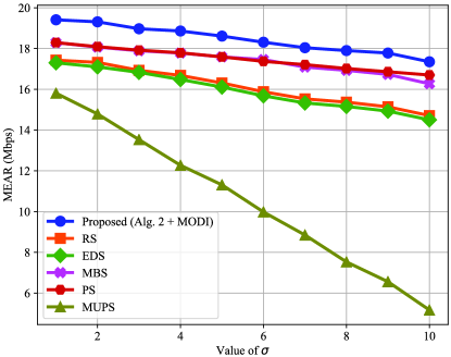
Figure 8: Comparison of average MEAR with varying value of $\sigma$ and $L=32$ Bytes.

In Fig. 10, we compare the average MEAR of eMBB UEs for considering varying uRLLC load ($L$) and uRLLC traffic ($\sigma$). The MEAR value of our method surpasses other concerned methods in every circumstance as revealed from Fig. 10. The same figure also explicates that these values degrade when $L$ increases for varying $\sigma$ as the system needs to allocate more PRBs to the uRLLC UEs. Moreover, these values decrease with the increasing value of $\sigma$ for a fixed $L$, and also the same for increasing the value of $L$ with a fixed $\sigma$. In Fig. 11, we compare the average fairness score of eMBB UEs for the different methods for changing the uRLLC load ($L$) and uRLLC traffic ($\sigma$). Fig. 11 exposes that the fairness scores of our method are better than or at least similar to that of its’ rivals. The figure also reveals that these scores decrease with an increasing $L$ for the lower value of $\sigma$. However, these scores increase with the increasing $L$ when $\sigma$ value is high. Moreover, for the MUPS method, these values decrease with the increasing value of $\sigma$ and $L$.

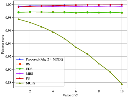
Figure 9: Comparison of fairness score with varying value of $\sigma$ and $L=32$ Bytes.

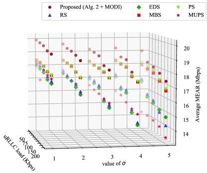
Figure 10: Comparison of average MEAR with varying uRLLC load and $\sigma$.

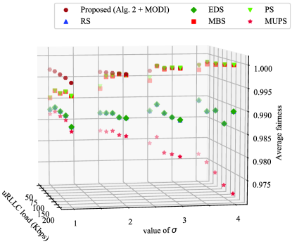
Figure 11: Comparison of average fairness score with varying uRLLC load and $\sigma$.

VI Conclusions

In this paper, we have introduced a novel approach for coexisting uRLLC and eMBB traffic in the same radio resource for enabling 5G wireless systems. We have expressed the coexisting dilemma as a maximizing problem of the MEAR value of eMBB UEs meanwhile attending the uRLLC traffic. We handle the problem with the help of the decomposition strategy. In every time slot, we resolve the resource scheduling sub-problem of eMBB UEs using a PSUM based algorithm, whereas the similar sub-problem of uRLLC UEs is unraveled through optimal transportation model, namely MCC and MODI methods. For the efficient scheduling of PRBs among eMBB UEs, we also present a heuristic algorithm. Our extensive simulation outcomes demonstrate a notable performance gain of the proposed approach over the baseline approaches in the considered indicators.

References

- [1] Cisco, “Cisco Visual Networking Index: Global Mobile Data Traffic Forecast Update, 2016 - 2021,” White Paper, June 2017.
- [2] 5G Forum, “5G Service Roadmap 2022,” White Paper, March 2016.
- [3] ITU-R, “IMT vision-framework and overall objectives of the future development of IMT for 2020 and beyond,” Recommendation M.2083-0, September 2015.
- [4] 3GPP, “3GPP TSG RAN WG1 Meeting #87,” November 2016.
- [5] 3GPP, “Downlink Multiplexing of eMBB and uRLLC Transmission,” 3GPP TSG RAN WG1 NR Ad-Hoc Meeting, R1-1700374, January 2017.
- [6] A. K. Bairagi, S. F. Abedin, N. H. Tran, D. Niyato, and C. S. Hong, “QoE-Enabled Unlicensed Spectrum Sharing in 5G: A Game-Theoretic Approach,” IEEE Access, vol. 6, pp.50538-50554, September 2018.
- [7] A. K. Bairagi, N. H. Tran, W. Saad, and C. S. Hong, “Bargaining Game for Effective Coexistence between LTE-U and Wi-Fi Systems,” in IEEE/IFIP Network Operations and Management Symposium (NOMS), Taipei, Taiwan, April 2018.
- [8] S. Liu, F. Yang, J. Song, and Z. Han, “Block Sparse Bayesian Learning-Based NB-IoT Interference Elimination in LTE-Advanced Systems,” IEEE Transactions on Communications, vol. 65, no. 10, pp. 4559-4571, October 2017.
- [9] S. F. Abedin, G. R. Alam, S.M. A. Kazmi, N. H. Tran, D. Niyato, and C. S. Hong, “Resource Allocation for Ultra-reliable and Enhanced Mobile Broadband IoT Applications in Fog Network,” IEEE Transactions on Communications, vol.67, no. 1, pp. 489-502, January 2019.
- [10] R. Kassab, O. Simeone and P. Popovski, “Coexistence of URLLC and eMBB Services in the C-RAN Uplink: An Information-Theoretic Study,” 2018 IEEE Global Communications Conference (GLOBECOM), Abu Dhabi, United Arab Emirates, 2018, pp. 1-6.
- [11] K. Ying, J. M. Kowalski, T. Nogami, Z. Yin, and J. Sheng, “Coexistence of enhanced mobile broadband communications and ultra-reliable low-latency communications in mobile front-haul,” Proc. SPIE 10559, Broadband Access Communication Technologies XII, 105590C, January 2018.
- [12] G. Pocovi, K. I. Pedersen, and P. Mogensen, “Joint Link Adaptation and Scheduling for 5G Ultra-Reliable Low-Latency Communications,” IEEE Access, vol. 6, pp. 28912-28922, May 2018.
- [13] P. Popovski, K. F. Trillingsgaard, O. Simeone, and G. Durisi, “5G Wireless Network Slicing for eMBB, URLLC, and mMTC: A Communication-Theoretic View,” in IEEE Access, vol. 6, pp. 55765-55779, September 2018.
- [14] H. Ji, S. Park, J. Yeo, Y. Kim, J. Lee, and B. Shim, “Ultra Reliable and Low Latency Communications in 5G Downlink: Physical Layer Aspects,” IEEE Wireless Communications, vol. 25, no. 3, pp. 124-130, June 2018.
- [15] M. Bennis, M. Debbah, and H. V. Poor, “Ultra-Reliable and Low-Latency Wireless Communication: Tail, Risk and Scale,” in Proceedings of the IEEE, vol. 106, no. 10, pp. 1834-1853, October 2018.
- [16] Q. Liao, P. Baracca, D. Lopez-Perez, and L. G. Giordano, “Resource Scheduling for Mixed Traffic Types with Scalable TTI in Dynamic TDD Systems,” in IEEE Globecom Workshops (GC Wkshps), Washington, DC, USA, December 2016.
- [17] K. I. Pedersen, G. Berardinelli, F. Frederiksen, P. Mogensen, and A. Szufarska, “A flexible 5G frame structure design for frequency-division duplex cases,” IEEE Communications Magazine, vol. 54, no. 3, pp. 53-59, March 2016.
- [18] K. Pedersen, G. Pocovi, J. Steiner, and A. Maeder, “Agile 5G Scheduler for Improved E2E Performance and Flexibility for Different Network Implementations,” IEEE Communications Magazine, vol. 56, no. 3, pp. 210-217, March 2018.
- [19] C. Li, J. Jiang, W. Chen, T. Ji, and J. Smee, “5G ultra-reliable and low-latency systems design,” in 2017 European Conference on Networks and Communications (EuCNC), Oulu, Finland, June 2017.
- [20] Z. Wu, F. Zhao, and X. Liu, “Signal Space Diversity Aided Dynamic Multiplexing for eMBB and URLLC Traffics”, in 3rd IEEE International Conference on Computer and Communication, Chengdu, China, December 2017.
- [21] A. Anand, G. Veciana, and S. Shakkottai, “Joint Scheduling of URLLC and eMBB Traffic in 5G Wireless Networks,” in IEEE International Conference on Computer Communications, Honolulu, USA, April 2018.
- [22] K. I. Pedersen, G. Pocovi, J. Steiner, and S. R. Khosravirad, “Punctured Scheduling for Critical Low Latency Data on a Shared Channel with Mobile Broadband,” in IEEE 86th Vehicular Technology Conference (VTC-Fall), Toronto, Canada, September 2017.
- [23] A. K. Bairagi, M. S. Munir, S. F. Abedin, and C. S. Hong , “Coexistence of eMBB and uRLLC in 5G Wireless Networks,” in Korea Computer Congress, Jeju, South Korea, June 2018.
- [24] A. K. Bairagi, M. S. Munir, M. Alsenwi, and C. S. Hong , “A Matching Based Coexistence Mechanism between eMBB and uRLLC in 5G Wireless Networks,” in 34th ACM/SIGAPP Symposium on Applied Computing (SAC 2019), Limassol, Cyprus, April 2019.
- [25] K. I. Pedersen, G. Pocovi, and J. Steiner, “Preemptive scheduling of latency critical traffic and its impact on mobile broadband performance,” in IEEE 87th Vehicular Technology Conference (VTC-Spring), Porto, Portugal, June 2018.
- [26] A. A. Esswie, and K. I. Pedersen, “Multi-user preemptive scheduling for critical low latency communications in 5G networks,” in IEEE Symposium on Computers and Communications (ISCC 2018), Natal, Brazil, June 2018.
- [27] A. A. Esswie, and K. I. Pedersen, “Opportunistic Spatial Preemptive Scheduling for URLLC and eMBB Coexistence in Multi-User 5G Networks,” IEEE Access, vol. 6, pp. 38451-38463, July 2018.
- [28] M. Alsenwi, N. H. Tran, M. Bennis, A. K. Bairagi, and C. S. Hong, “eMBB-URLLC Resource Slicing: A Risk-Sensitive Approach,” IEEE Communications Letters, vol. 23, no. 4, pp. 740-743, April. 2019.
- [29] 3GPP, “Study on New Radio Access Technology Physical Layer Aspects,” Document 3GPP RT 38.802v14.0.0, March 2017.
- [30] J. Scarlett, V. Y. F. Tan, and G. Durisi, “The dispersion of nearest-neighbor decoding for additive non-gaussian channels,” IEEE Transactions on Information Theory, vol. 63, no. 1, pp. 81–92, January 2017.
- [31] N. Zhang, Y. F. Liu, H. Farmanbar, T. H. Chang, M. Hong, and Z. Q. Luo, “Network Slicing for Service-Oriented Networks Under Resource Constraints,” IEEE Journal on Selected Areas in Communications, vol. 35, no. 11, pp. 2512–2521, November 2017.
- [32] P. Liu, Y. F. Liu, and J. Li, “An iterative reweighted minimization framework for joint channel and power allocation in the OFDMA system,” in 2015 IEEE International Conference on Acoustics, Speech and Signal Processing (ICASSP), South Brisbane, Australia, April 2015.
- [33] D. R. Hunter, and K. Lange, “A Tutorial on MM Algorithms,” The American Statistician, vol. 58, no. 1, pp. 30–37, February 2004.
- [34] M. Razaviyayn, M. Hong, and Z. Luo, “A Unified Convergence Analysis of Block Successive Minimization Methods for Nonsmooth Optimization,” SIAM Journal on Optimization, vol. 23, no. 2, pp. 1126–1153, June 2013.
- [35] F. L. Hitchcock, “The Distribution of a Product from Several Sources to Numerous Localities”,Journal of Mathematics and Physics, vol. 20, no. 1-4, pp. 224–230, April 1941.
- [36] G.B. Dantzig, “Linear Programming and Extensions”, Princeton University Press, Princeton, N J, 1963.
- [37] N.V. Reinfeld, and W.R. Vogel, “Mathematical Programming”,Prentice-Hall, Englewood Gliffs, New Jersey, 1958.
- [38] D.G. Shimshak, J.A. Kaslik, and T.D. Barclay, “A modification of Vogel’s approximation method through the use of heuristics”,Information Systems and Operational Research, vol. 19, no. 3, pp. 259-263, 1981.
- [39] A. Charnes, and W. W. Cooper, “The Stepping Stone Method of Explaining Linear Programming Calculations in Transportation Problems”,Management Science, vol. 1, no. 1, pp. 1–102, October 1954.
- [40] H. A. Taha, “Operations Research: An introduction”, Pearson Education, Inc., Upper Saddle River, New Jersey, 2007.
- [41] R. Jain, D.M. Chiu, and W.R. Hawe, “A quantitative measure of fairness and discrimination for resource allocation in shared computer system,” Eastern Research Laboratory, Digital Equipment Corporation, vol. 38, September 1984.