Slice Tuner: A Selective Data Acquisition Framework for Accurate and Fair Machine Learning Models

Abstract.

As machine learning becomes democratized in the era of Software 2.0, a serious bottleneck is acquiring enough data to ensure accurate and fair models. Recent techniques including crowdsourcing provide cost-effective ways to gather such data. However, simply acquiring data as much as possible is not necessarily an effective strategy for optimizing accuracy and fairness. For example, if an online app store has enough training data for certain slices of data (say American customers), but not for others, obtaining more American customer data will only bias the model training. Instead, we contend that one needs to selectively acquire data and propose Slice Tuner, which acquires possibly-different amounts of data per slice such that the model accuracy and fairness on all slices are optimized. This problem is different than labeling existing data (as in active learning or weak supervision) because the goal is obtaining the right amounts of new data. At its core, Slice Tuner maintains learning curves of slices that estimate the model accuracies given more data and uses convex optimization to find the best data acquisition strategy. The key challenges of estimating learning curves are that they may be inaccurate if there is not enough data, and there may be dependencies among slices where acquiring data for one slice influences the learning curves of others. We solve these issues by iteratively and efficiently updating the learning curves as more data is acquired. We evaluate Slice Tuner on real datasets using crowdsourcing for data acquisition and show that Slice Tuner significantly outperforms baselines in terms of model accuracy and fairness, even when the learning curves cannot be reliably estimated.

1. Introduction

In the era of Software 2.0 (kar, [n.d.]), machine learning (ML) is becoming democratized where successful applications range from recommendation systems to self-driving cars. Software engineering itself is going through a fundamental shift where trained models are the new software, and data becomes a first-class citizen on par with code (Polyzotis et al., 2018). Training a model to use in production requires multiple steps including data acquisition and labeling, data analysis and validation, model training, model evaluation, and model serving, which can be a complicated process for ML developers. In response, end-to-end ML platforms (Baylor et al., 2017; Zaharia et al., 2018) that perform all of these steps have been proposed.

As ML applications become more diverse and possibly narrow, acquiring enough training data is becoming one of the most critical bottlenecks. We explicitly use the terminology data acquisition to make a distinction with the broader problem of data collection (Roh et al., 2019), which also includes labeling existing data as in active learning (Settles, 2012) or weak supervision (Ratner et al., 2019). Instead in data acquisition, the goal is to obtain the right amounts of new data from other data sources. Unlike well-known problems like machine translation where there is decades’ worth of parallel corpora to train models, most new applications have little or no training data to start with. For example, a smart factory application for quality control may need labeled images of its own specific products. In response, there has been significant progress in data acquisition research (Roh et al., 2019) including dataset discovery (Nargesian et al., 2019), crowdsourcing (ama, [n.d.]), and even simulator-based data generation (Kim et al., 2019). As a result, it is reasonable to assume that new training data can now be acquired at will given enough budget.

When acquiring data for ML, a common misconception is that more data leads to better models. However, this claim does not always hold when the goal is to improve both the model accuracy and fairness, which are not always aligned. Let us divide the data into subsets called slices. For example, a company selling apps online may divide its customer purchase data by region as shown in Figure 1 (each box indicates a slice where the height is the slice’s size). Say that the company not only wants to ensure that its app recommendations are accurate overall, but evenly accurate (i.e., fair) for customers in different regions. Since the company already has enough data for American customers (the slice size is largest), acquiring more American customer data (gray part in Figure 1(a)) is not only unnecessary, but may bias the training data and influence the model’s accuracy on other regions.

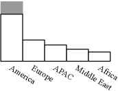
(a)

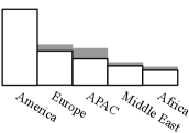
(b)

Figure 1. Customer slices in different regions where the boxes represent the initial slices (height = slice size) while the gray bars on top indicate the amounts of acquired data per slice. (a) If there is already enough American customer data, acquiring more of it may worsen the data bias. (b) Instead, it is better to acquire possibly-different amounts of data for slices to optimize both the model accuracy and fairness on all slices.

We thus propose a selective data acquisition framework called Slice Tuner, which determines how much data to acquire for each slice. Not all slices have the same data acquisition cost-benefits, which means that acquiring the same amounts of data may result in different improvements in model loss for different slices. Hence, the naïve strategy of acquiring equal amounts of data per slice is not necessarily optimal. Alternatively, acquiring data such that all slices end up having equal amounts of training data is not always optimal either. (This approach is similar to the Water filling algorithm (Proakis, 2007); details in Section 2.2.) Instead, we would like a data acquisition strategy such that the models are accurate and similarly-accurate for different slices. To measure model accuracy, we use loss functions like logistic loss. For fairness we use an extension of equal error rates (Venkatasubramanian, 2019; Zafar et al., 2017), which is one of the widely-accepted definitions of fairness along with other traditional ones like demographic parity (Feldman et al., 2015) and equalized odds (Hardt et al., 2016). Interestingly, equal error rates is a familiar concept in systems research where it is important to have similar performance across different partitions of data. The key challenge is to figure out the different cost benefits of the slices and estimate how much data to acquire for each slice given a budget. In Figure 1(b), we may want to acquire even amounts of data only for non-America regions.

At the core of Slice Tuner is the ability to estimate the learning curves of slices, which reflect the cost benefits of data acquisition. It is well known that the impact of data acquisition on model loss is initially large, but eventually plateaus (Sheng et al., 2008). That is, lowering the loss becomes difficult to the point where it is not worth the data acquisition effort. Figure 2 shows hypothetical learning curves of two slices. Recently, multiple studies (Chen et al., 2018; Hestness et al., 2017; Domhan et al., 2015) show that these curves usually follow a power law according to empirical results in machine translation, language modeling, image classification, and speech recognition. Given the learning curves, Slice Tuner “tunes” the slices by determining how much data to acquire for each slice such that the model accuracy and fairness on all slices are optimized while using a limited budget for data acquisition.

Figure 2. Hypothetical learning curves of two slices.

As a toy example, suppose there are two slices $s_{1}$ and $s_{2}$ of the same size. Say the current model losses of the two slices are 5 and 3, respectively. Hence, the loss of the entire data is 4. According to Definition 1 in Section 2.1, we compute the unfairness as avg$\left\{|5-4|,|3-4|\right\}=1$. Now suppose we estimate their two learning curves as shown in Figure 2. Notice that the curve of $s_{2}$ is rather flat, so acquiring more data does not have as much benefit as acquiring for $s_{1}$. Suppose we have a budget of acquiring examples using crowdsourcing. Since $s_{1}$ has a better cost-benefit, we may decide to only acquire examples for $s_{1}$. The actual numbers would depend on the result of the optimization problem. As a result, say the model losses of $s_{1}$ and $s_{2}$ are now 2 and 3, respectively, and that the entire data now has a loss of 2.4 ($s_{1}$ is now larger than $s_{2}$, so the average loss is closer to 2 than 3). In that case, the unfairness improves by decreasing to avg$\left\{|2-2.4|,|3-2.4|\right\}=0.5$.

While learning curves are potentially useful, in reality we cannot assume they will be generated in perfection. Instead, the key technical challenge we address is generating learning curves that are “reliable enough” to still benefit Slice Tuner using data management techniques. There are largely two obstacles. First, slices may not have enough data for the model losses to be precisely measured. Second, acquiring data for one slice may “influence” the model’s losses on other slices and thus distort their learning curves. Slice Tuner solves these problems by iteratively updating the learning curves as more data is acquired so that the learning curves are up-to-date. In addition, Slice Tuner exploits the learning curves by doing a relative comparison of losses, so perfectly predicting the absolute losses in each learning curve is not necessary.

In our experiments, we use various real datasets to show that Slice Tuner outperforms other baselines in terms of model loss and unfairness, even when the learning curves are not reliable. We also demonstrate the real scenario of acquiring new data using crowdsourcing via Amazon Mechanical Turk (ama, [n.d.]) for the image dataset UTKFace (Zhang et al., 2017) and show that Slice Tuner is effective even if the data is acquired from a completely different data source.

A remaining question is how to define the slices themselves. Data slicing can either be done manually (tfm, [n.d.]) or automatically (Chung et al., 2019). While Slice Tuner can run on any set of slices, a desirable property of a slice is to be unbiased such that acquiring any example that belongs to it has a similar effect on model loss as any other possible example. In this work, we assume the slices are provided by the user, but also discuss possible solutions in Appendix  A.

To democratize ML, it is important to help users to not only analyze their models, but also fix any problems easily. To our knowledge, Slice Tuner is the first system to provide concrete action items of how much data to acquire per slice to make models both accurate and fair. We also release our code and crowdsourced dataset as a community resource (git, [n.d.]).

The rest of the paper is organized as follows:

• We cover preliminaries and formulate the problem of selective data acquisition (Section 2).

• We describe Slice Tuner’s architecture (Section 3).

• We propose accurate and efficient methods for estimating the learning curves of slices (Section 4).

• We propose selective data acquisition algorithms (Section 5).

• We evaluate Slice Tuner on real datasets and show that it outperforms baselines by obtaining better model accuracy and fairness results using the same data acquisition budget, even if the learning curves cannot be reliably estimated (Section 6).

2. Problem Definition

2.1. Preliminaries

Data Slicing

We denote by $D$ the training data set with examples where each example $e\in D$ has features and a label. Without loss of generality, we assume all examples have equal weights when training a model. $D$ can be divided into slices $S=\{s_{i}\}_{i=1}^{n}$ where each $s_{i}\subseteq D$. We assume that the slices partition $D$, i.e., $\bigcup_{i}s_{i}=D$. A typical way to define a slice is to use conjunctions of feature-value pairs, e.g., $region=Europe\wedge gender=Female$. We can also use the label feature for the slicing. For example, the Fashion-MNIST dataset (Xiao et al., 2017) contains images that represent items, e.g., shoes and shirts. Here, we can define a slice for each item. The slices can be found automatically or set manually by a domain expert. Although there is no restriction in defining a slice, a desirable property is that the slice is unbiased such that adding a new example to it has a similar effect on the model accuracy as any other example. We assume the slices are provided by users, but also discuss possible solutions in Appendix  A where the idea is to iteratively divide slices until they are unbiased using decision tree methods.

Model Accuracy and Fairness Measures

We assume a model $M$ is trained on $D$ or its subsets. We also assume a classification loss function $\psi(s,M)$ that returns a performance score on how well $M$ predicts the labels of the dataset $s$. A common loss function for binary classification is log loss, which is $\frac{1}{m}\sum_{i=1}^{m}-y^{(i)}\log\hat{y}^{(i)}-(1-y^{(i)})\log(1-\hat{y}^{(i)})$. Our setting can be generalized to other ML problems (multi-class classification and regression) by using the appropriate loss functions. Throughout the paper, we will use loss to measure accuracy.

Our notion of fairness extends equalized error rates (Venkatasubramanian, 2019), which has the definition $Pr(\hat{y}\neq y|z=0)\approx Pr(\hat{y}\neq y|z=1)$ where $\hat{y}$ is the model prediction, $y$ is the label, and $z$ is a sensitive attribute like gender. We make the straightforward extension that the model error rates must be similar among any number of groups that are not necessarily defined with sensitive attributes. Equalized error rates is one of the standard fairness measures along with demographic parity (Feldman et al., 2015) and equalized odds (Hardt et al., 2016). We choose equalized error rates because it is important for any ML product that needs to provide similar service quality to customers of different demographics. This fairness is also a familiar notion in systems research where a system should perform well on different partitions of data.

We propose the following unfairness measure that is used to obtain equalized error rates:

Definition 0.

The unfairness of the slices is defined as the average absolute difference between the loss of a slice and the entire data $D$:

$$\mathrm{avg}_{s_{i}\in S}|\psi(s_{i},M)-\psi(D,M)|.$$

Notice that the unfairness measure does not require sensitive attributes and can thus be used on any dataset. We can also think of other variations such as computing the maximum absolute difference instead of the average.

Data Acquisition Cost

We assume that any data acquisition technique can be used to acquire data by paying a certain cost. Nowadays, dataset discovery systems (Nargesian et al., 2019) can help find relevant datasets. In addition, crowdsourcing tools like Amazon Mechanical Turk (ama, [n.d.]) or real-world simulators (Kim et al., 2019) can be used to generate data at will.

We abstract the data acquisition methods and define a cost function $C(s)$ that returns the cost to acquire an example in slice $s$. Even for the same data source, the data acquisition cost may vary by slice. For example, acquiring face images of large groups (e.g., $race=White$) may be easier than images of smaller groups (e.g., $race=Native\ Hawaiian$). We assume that within the same slice, the cost to acquire an example is the same. As more examples are acquired for $s$, $C(s)$ may increase possibly because data becomes scarcer. However, we assume that data is acquired in batches (e.g., when using Amazon Mechanical Turk, we use a fixed budget at a time) and that $C(s)$ is a constant for each batch.

Slice Dependencies

Slices may have dependencies where acquiring data for one slice may influence the learning curves of other slices. For example, if there are two independent slices $s_{1}$ and $s_{2}$, and we acquire too much data for $s_{1}$, the model may overfit and have a worse accuracy on $s_{2}$. If $s_{2}$ is similar to $s_{1}$ content-wise, then the accuracy on $s_{2}$ can actually increase as well. If there are no dependencies, the slices are considered independent of each other. We discuss how to handle slice dependencies in Section 5.2.

2.2. Selective Data Acquisition

We now define the problem of selective data acquisition.

Definition 0.

Given a set of examples $D$, its slices $S=\{s_{i}\}_{i=1}^{n}$, a trained model $M$, a data acquisition cost function $C$, and a data acquisition budget $B$, the selective data acquisition problem is to acquire $d_{i}$ examples for each slice $s_{i}\in S$ such that the following are all satisfied:

• The average loss $\psi(D,M)$ is minimized,

• The unfairness $\mathrm{avg}_{s_{i}\in S}|\psi(s_{i},M)-\psi(D,M)|$ is minimized, and

• The total data acquisition cost $\sum_{i}C(s_{i})\times d_{i}=B$.

We note that minimizing loss and unfairness are correlated, but not necessarily the same and thus need to be balanced (Section 6.3.2 studies the tradeoffs). In some cases, making sure slices have similar losses may also result in the lowest loss. For example, if there are two independent slices with identical learning curves, and one of them has less data, then simply making the two slices have the same amount of data results in the optimal solution. However, there are cases where the two objectives are not aligned. Continuing our example, suppose that the two slices now have different learning curves where the slice with less data has a curve that is lower than the other curve and also decreases more rapidly. In this case, acquiring data for the smaller slice would lower loss, but increase unfairness. Instead, the optimal solution could be to also acquire some data for the larger slice to lower the loss without sacrificing too much fairness.

Our problem can be viewed as a special type of multi-armed bandit problem as we discuss in Section 7.

Baselines for Comparison

Recall we described two data acquisition baselines in Section 1. Both methods are reasonable starting points, but do not optimally solve our problem in Definition 2. Suppose there are two independent slices $s_{1}$ and $s_{2}$. The first baseline is to acquire equal amounts of data for all slices (Figure 3(a)). This approach does not perform well if the two slices have significantly different learning curves. In a worst-case scenario, $s_{1}$ may already have a low loss and does not need more data acquisition whereas $s_{2}$ may have a high loss and can benefit from more data. In this case, acquiring equal amounts of data will result in both suboptimal loss and unfairness. The second baseline is to acquire data such that all slices have similar amounts of data in the end, which can be viewed as a Water filling algorithm (Figure 3(b)). The implicit assumption is that all slices require similar amounts of data to obtain similar losses. However, this assumption does not hold if the two slices have different losses even if they have the same size. Continuing from the above worst-case scenario, if $s_{1}$ is smaller than $s_{2}$, then we will end up acquiring data for $s_{1}$ unnecessarily and again get suboptimal results. What we need instead is a way to utilize the learning curves and solve an optimization problem to determine how much data to acquire for each slice.

(a)

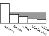
(b)

Figure 3. The two baselines for data acquisition: (a) acquire similar amounts of data per slice, (b) acquire data such that the slices have similar sizes in the end (Water filling alg.).

Another possible baseline is to acquire data in proportion to the original data distribution (Chen et al., 2018). However, this approach does not fix data bias at all, so we considered it strictly worse than the baselines above. Also, we re-emphasize that active learning is not a comparable technique because it labels existing data instead of acquiring new data.

3. System Overview

We describe the overall workflow of Slice Tuner as shown in Figure 4. Slice Tuner receives as input a set of slices and their data and estimates the learning curves of the slices by training models on samples of data. We explain the details of the estimation methods in Section 4. Next, Slice Tuner performs the selective data acquisition optimization where it determines how much data should be acquired per slice in order to minimize the loss and unfairness. As data is acquired, the learning curves can be iteratively updated. We propose selective data acquisition algorithms in Section 5.

Figure 4. The input of Slice Tuner are the slices with their data. Slice Tuner consists of two main components: the Learning Curve Estimator and Selective Data Acquisition Optimizer. The learning curves may be iteratively updated as more data is acquired by the Data Acquisition component. Slice Tuner suggests how much data to acquire per slice.

We discuss the runtime requirements of Slice Tuner. Looking at Figure 4, we consider the Data Acquisition step to be the most expensive process done as a batch process, especially if manual crowdsourcing is used. Even if there are tools for dataset searching and simulation, there is still a fair amount of manual work involved. As a result, it is critical for Slice Tuner to minimize the amount of data acquisition at the expense of possibly using more computation for estimating learning curves and performing the optimization.

4. Learning Curve

A learning curve is a projection of how a model trained on the entire dataset will perform on a particular slice $s$ as a function of the number of examples in $s$. Assuming that the examples are helpful to the model training, we expect the loss to decrease as more examples are added. However, this trend may not always hold due to multiple factors: the examples may be noisy and actually harm the model training, the examples may be biased and only represent a small part of the slice, or the model training itself may be unstable, all of which may result in non-monotonic behavior. Despite the complexity, we believe it is reasonable to assume that more training data on an unbiased slice generally leads to lower loss, but that the benefits have diminishing returns. Unlike existing work, a significant challenge for Slice Tuner is to plot the learning curves on slices, which can be arbitrarily smaller than the entire data. We first discuss how to efficiently estimate learning curves using data management in this section and then how to handle unreliable learning curves in Section 5.

4.1. Estimation

A key property we exploit is that training data benefits the model accuracy, but more collection has diminishing returns. A recent work from Baidu (Hestness et al., 2017) conducted an analysis on learning curves (see Figure 5). The curve starts with the small-data region, where models try to learn from a small number of training data and can only make “best guess” predictions. According to our experience, tens of examples is enough to move beyond this region. For more data, we can see a power-law region of the form $y=bx^{-a}$, where new training examples provide useful information to improve the predictions. For real-world applications, a lower bound error may exist due to errors such as mislabeled data that cause incomplete generalization. Hence, we then see a diminishing-returns region where there is a minimum loss that cannot be reduced. In this case, one may also model the learning curve using the form $y=bx^{-a}+c$ (Hestness et al., 2017) where $c$ is the lower-bound loss. However, if not enough data has been acquired to observe diminishing returns, fitting the curve $y=bx^{-a}$ works better (Hestness et al., 2017). Another study (Domhan et al., 2015) compares 11 parametric models including variations of exponential models and custom models. Based on these works, a power-law curve fits as well as any other curve.

Figure 5. A detailed view of how loss changes against more training data based on work by Baidu (Hestness et al., 2017). There are three regions: (1) small-data region: the slice is too small to the extent that the model predictions are more or less random, (2) power-law region: the curve is of the form $y=bx^{-a}$, and (3) diminishing-returns region: there is enough data, so acquiring more does not help reduce the loss.

To fit a learning curve of a slice, we first divide its data into train and validation sets. Although the train set may be small, we do assume a validation set that is large enough to evaluate models. This assumption is reasonable in the common setting where we start with some initial data and would like to acquire more examples. We then train models on random subsets of the train set with different sizes and generate data points by evaluating the models on the validation set. How many data points to generate depends on how much time we are willing to invest to estimate the learning curve. Each time we train a model on a subset of data, we also combine that data with the rest of the slices. (Section 4.2 presents a more efficient method for generating data points.) Since the model losses on smaller subsets are less reliable (depicted as having high variance Figure 5), we give weights to subsets that are proportional to their sizes and use a non-linear least squares method (Figueroa et al., 2012) for curve fitting. We further improve reliability by drawing multiple curves (we use 5) and averaging them at the expense of more computation.

In the worst case when all subsets are in the small-data region, then Slice Tuner may not benefit from learning curves, but in that case would fall back to performing like baselines. If there is enough data in a slice to be in the diminishing return region, we do not need to do any special handling because Slice Tuner will simply acquire data for other slices that need more data.

4.2. Efficient Implementation

We now discuss better data management techniques for more efficient learning curve fitting. Given the slices $S$, suppose we generate for each slice $K$ random subsets of data to fit a power-law curve. In addition, we may repeatedly update the learning curves $U$ times using our iterative algorithms in Section 5.2. We would thus have to train a model $|S|\times K\times U$ times. A typical setting in our experiments is $|S|=10$, $K=10$, and $U=5$, which means that we may train a model 500 times. Moreover, if we train a model on a subset of a slice plus the rest of the slices, then the rest of the slices could be relatively too large for the model to properly train on the subset due to the data bias. Moreover, each model training may take a long time because the rest of the slices are repeatedly used for training in their entirety.

We thus propose an amortization technique to drastically reduce the number of model trainings. Instead of taking an X% subset of one slice and leaving the rest as is to train each model, we take X% subsets of all slices and train a model. This model is then evaluated on each of the slices to generate different learning curves independently. This approach assumes that taking subsets of other slices does not affect the model accuracy on the current slice. In reality, this independence assumption does not hold, so Slice Tuner solves the problem by periodically updating the learning curves as we explain in Section 5.2. As a result, the number of model trainings becomes independent of the number of slices and reduces to $O(K\times U)$. In our example above, number 500 reduces to about 50. In addition, each model training is on average faster than the exhaustive approach above because it is performed on smaller data (X% subsets). Finally, the learning curves can be generated in parallel, so using more nodes further reduces the wall-clock time.

Another possible optimization is to use a chain of transfer learning where a model trained on one subset is re-used to train the model of the next subset faster and so on. This approach has the potential to reduce the average model training time, although the time complexity remains the same. However, a downside is that hyperparameter tuning becomes significantly more complicated where we may need to use different learning rates for subsequently-trained models, so we do not use this optimization in our experiments.

5. Selective Data Acquisition

We first tackle the selective data acquisition problem to minimize model loss and unfairness when slices are independent of each other and then extend our methods to the case where slices may influence each other.

5.1. Independent Slices

We first assume that slices do not influence each other. Hence, we only need to solve the optimization problem once. The optimization should be done on all slices as our objective for minimizing loss and unfairness is global. We can formulate a convex optimization problem for selective data acquisition as follows. For the slices $\{s_{i}\}_{i=1}^{n}$ with sizes $\{|s_{i}|\}_{i=1}^{n}$, we want to find the number of examples to acquire for the slices $\{d_{i}\}_{i=1}^{n}$ to minimize the objective function using a total budget of $B$. We assume that the model’s loss on a slice follows a power-law curve of the form $b_{i}(|s_{i}|+d_{i})^{-a_{i}}$ where $b_{i}$ and $a_{i}$ are positive values. We define $A$ to be the average loss across all slices and $C(s_{i})$ to be the cost function that captures the effort to acquire an example for $s_{i}$. The optimization problem is then

$$\min\sum_{i=1}^{n}b_{i}(|s_{i}|+d_{i})^{-a_{i}}+\lambda\sum_{i=1}^{n}\max\left\{0,\frac{b_{i}(|s_{i}|+d_{i})^{-a_{i}}}{A}-1\right\}$$

$$\text{subject to}\sum_{i=1}^{n}C(s_{i})\times d_{i}=B$$

where the first term minimizes the loss, and the second term minimizes unfairness by giving a penalty to each slice $s_{i}$ that has a higher loss than $A$. If the loss of $s_{i}$ is lower than $A$, we return 0 to prevent the second term from giving a negative value. Since minimizing loss and unfairness are not always aligned, we introduce the $\lambda$ term to balance between minimizing each of them. By acquiring data for slices with higher losses, we eventually satisfy Definition 1.

This problem is convex assuming that the model’s loss decreases monotonically against more data. The first loss term $b_{i}(|s_{i}|+d_{i})^{-a_{i}}$ is a convex function of $d_{i}$ because it is a power-law curve. The second unfairness term is also convex because $b_{i}(|s_{i}|+d_{i})^{-a_{i}}$ is convex, $A$ is a constant for the current $D$, and taking a maximum between two convex functions is convex. Finally, $C(s_{i})$ is a constant that varies by slice. Hence, we can derive an optimal solution efficiently using any off-the-shelf convex optimization solver.

Algorithm

The One-shot algorithm updates the learning curves using the techniques in Section 4.2 and solves the above optimization problem to determine how much data to acquire for each slice. Note that One-shot always uses the entire budget $B$, assuming the learning curves are perfect, and the slices are independent.

5.2. Dependent Slices

We now consider the case where slices can influence each other. Suppose that there are two slices $s_{1}$ and $s_{2}$. If we acquire data for $s_{1}$ such that it dominates $s_{2}$ in quantity, then the model training may overfit on $s_{1}$. Consequently, the model accuracy on $s_{2}$ may change. Hence, we need to iteratively update the learning curves as more data is acquired. Notice that the iterative updates also serve the dual purpose of making the learning curves more reliable.

Modeling the Influence

(a)

(b)

(c)

Figure 6. (a) Consider three slices where shape indicates slice, and color indicates label. (b) If we evenly increase the data for all slices, the bias does not change much, and there is little influence among slices. (c) If we only increase the white triangles, the decision boundary may shift to the left due to the new bias, decreasing the loss for the white squares and increasing the loss for the black circles.

We hypothesize that the relative sizes of the slices (i.e., the bias) and the data similarities between slices play major roles. Figure 6 shows a synthetic example to demonstrate this point. Suppose that we start with three slices (circle, triangle, and square) in Figure 6(a) where the colors (black and white) indicate the labels. The straight line indicates the decision boundary of the model. Now suppose we evenly increase the data for all slices by 50% as shown in Figure 6(b). Since the bias does not change, the decision boundary does not change much either, which means that there is little influence on any of the slices. However, if we only increase the size of the triangle slice as shown in Figure 6(c), suppose the new bias causes the decision boundary to shift towards the left and influences the losses of the square and circle slices. The direction of influence depends on the similarity of data among slices. In our case, the square slice has the same label values as the triangle slice, and its loss decreases as all examples are categorized correctly. On the other hand, the circle slice has different label values than the triangle slice, and its loss increases.

To verify our hypothesis, we perform an experiment on the real UTKFace dataset (Zhang et al., 2017) where we use slices that represent different race and gender combinations of people (more details in Section 6.1). We use imbalance ratio (Buda et al., 2018), which is the maximum ratio between any two slices in $S$, as a proxy for bias. For example, if the slices $s_{1}$, $s_{2}$, and $s_{3}$ have sizes 10, 20, and 30, respectively, then the imbalance ratio is $\frac{max\{10,20,30\}}{min\{10,20,30\}}$ = $\frac{30}{10}$ = 3. We also define influence on a slice as the change in loss. According to our hypothesis, if the imbalance ratio changes, the magnitude of influence increases as well. We then observe the affect of imbalance ratio on influence as shown in Figure 7. Initially, all the slices are of the same size 300, except for the slice White_Male, which starts from size 50. As we add more examples only to White_Male, the imbalance ratio change increases, causing the influences on other slices to increase in magnitude as well. While most slices have increasing losses, only the slice White_Female shows decreasing losses because it has similar data. We make similar observations in other datasets as well.

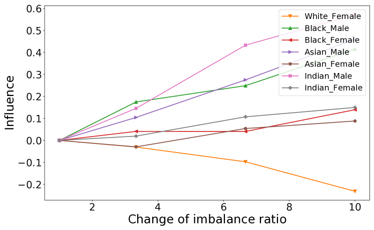
Figure 7. The influences (loss changes) of other UTKFace data slices as more data is acquired for White_Male, starting from size 300. As the change of the imbalance ratio increases, so does the magnitude of influences on other slices.

Algorithm

We iteratively update the learning curves whenever ”enough” influence occurs, regardless of its direction. The Iterative algorithm (shown in Algorithm 1) limits the change of imbalance ratio to determine how much data to acquire for each slice. We obtain the slice sizes and initialize the imbalance ratio absolute change limit $T$ to 1. While there is enough budget for data acquisition, we increase $T$ per iteration using one of the strategies discussed later. The parameter $L$ specifies the minimum slice sizes to start with and is positive. If any slice is smaller than $L$, we acquire enough examples assuming there is enough budget. (In Section 6.3.4, we show that $L$ can be a small value.) We then run the One-shot algorithm to derive how many examples to acquire for each slice if we use the entire budget $B$. If the imbalance ratio change would exceed $T$ if we use the entire budget, we limit the number of examples acquired by multiplying $num\_examples$ with the maximum ratio that would not allow that to happen ($change\_ratio$). This problem has nonlinear constraints, and the GetChangeRatio function uses an off-the-shelf optimization library in SciPy to derive a solution. After reflecting $B$, $T$, and $IR$, we repeat the same steps until we run out of budget.

For example, suppose $L=10$, and there are two slices $s_{1}$ and $s_{2}$ with initial sizes of 5 and 10 (i.e., $sizes=[5,10]$) with a budget of $B=55$. First, we need to acquire 5 examples for $s_{1}$ (i.e., $num\_examples$ = [5, 0]) to satisfy $L$ (Step 4). Then we update $sizes$ to $[10,10]$ and $B$ to 50 (Steps 5–6). Then we set $IR$ to $\frac{10}{10}=1$. After running One-shot, suppose that $num\_examples$ = [10, 40] (Step 9). If we acquire all this data, the imbalance ratio would become $\frac{10+40}{10+10}=2.5$, so $|After\_IR-IR|$ = 2.5 - 1 = 1.5. To avoid exceeding $T=1$, we compute the change ratio $x$ such that $\frac{10+40x}{10+10x}=2$ by invoking the GetChangeRatio function (Step 13). The solution is $x=0.5$, and $num\_examples$ thus becomes $0.5\times[10,40]=[5,20]$. After acquiring the data, we update $sizes$, $B$, $T$, and $IR$ and go back to Step 8.

Input: The slices $S$, budget $B$, minimum slice size $L$, and data acquisition cost function $C$

1 $sizes$ = SliceSizes($S$);

2 $T$ = 1;

3 if $\exists i\ sizes[i]<L$ then

       /* Ensure minimum slice size L */

4       $num\_examples$ = $\max(L\times{\bf 1}-sizes,0)$;

5       $sizes$ = $sizes$ + $num\_examples$;

6       $B$ = $B$ - $\sum_{i}(C(i)\times num\_examples[i])$;

7      

8$IR$ = GetImbalanceRatio($sizes$);

9 while $B>0$ do

       /* One-shot always uses the entire budget */

10       $num\_examples$ = OneShot($sizes$, $B$);

11       $After\_IR$ = GetImbalanceRatio($sizes+num\_examples$);

12      

13      if $|After\_IR-IR|>T$ then

             /* Do not make imbalance ratio change exceed T */

14             $target\_ratio$ = $IR+T\times$ Sign($After\_IR-IR$);

15             $change\_ratio$ = GetChangeRatio($sizes$, $num\_examples$, $target\_ratio$);

16             $num\_examples$ = $change\_ratio\times num\_examples$;

17             $After\_IR$ = GetImbalanceRatio($sizes+num\_examples$);

18            

19      CollectData($num\_examples$);

20       $sizes$ = $sizes$ + $num\_examples$;

21       $B$ = $B$ - $\sum_{i}(C(i)\times num\_examples[i])$;

22       $T$ = IncreaseLimit($T$);

23       $IR$ = $After\_IR$;

24      

25return;

26 Function GetImbalanceRatio($sizes$):

27       return $\frac{\max(sizes)}{\min(sizes)}$;

28      

ALGORITHM 1 Iterative algorithm for Slice Tuner

We now discuss strategies for updating the limit $T$ per iteration using the IncreaseLimit function. On one hand, it is desirable to minimize the number of iterations of Algorithm 1 because each iteration invokes the One-shot algorithm, which involves updating the learning curves and solving an optimization problem. On the other hand, we would like to update the learning curves to be as accurate as possible. While there are many ways to update $T$, we propose the following representative strategies:

• Conservative: For each iteration, leave $T$ as a constant, which limits the imbalance ratio to change linearly. The advantage is that we can avoid mistakenly acquiring too much data due to inaccuracies in the learning curves. However, the number of iterations may be high.

• Moderate: For each iteration, increase $T$ by a constant $c$. Compared to Conservative, this approach reduces the number of iterations, but may acquire data unnecessarily.

• Aggressive: For each iteration, multiply $T$ by a constant $c>1$. Compared to Moderate, this strategy collects data even more aggressively using possibly fewer iterations.

6. Experiments

In this section, we evaluate Slice Tuner on real datasets and address the following questions:

• How reliable and efficient is the learning curve generation used in Slice Tuner?

• How does Slice Tuner compare with the baselines in terms of model loss and unfairness?

• How does Slice Tuner perform on small slices where the learning curves are unreliable?

Slice Tuner is implemented in TensorFlow (Abadi et al., 2016) and Keras, and we use Titan RTX GPUs for model training.

6.1. Setting

Datasets

We experiment on the following four datasets that capture different characteristics of the slices. While the AdultCensus dataset is the most widely-used in the fairness literature, Slice Tuner is not limited to any particular dataset because our unfairness measure (Definition 1) does not require sensitive attributes (e.g., race and gender).

• Fashion-MNIST (Xiao et al., 2017): Contains images that can be categorized as one of 10 type of clothes, e.g., shoes, shirts, pants, and more. Here we slice the images according to their labels, i.e., there are 10 slices in total.

• Mixed-MNIST: Combines the Fashion-MNIST dataset and MNIST dataset(LeCun et al., 2001), which contains images that represent digits from 0 to 9. Created to demonstrate a dataset with a large number (20) of non-homogeneous slices from two data sources.

• UTKFace (Zhang et al., 2017): Contains various face images of people of different (male and female) gender and race (White, Black, Asian, and Indian), used for race classification. We used 8 slices by combining two genders and four races, e.g., Black female.

• AdultCensus (Kohavi, 1996): Contains people records with features including age, education, and sex. Used to predict which people make over $50K per year. We use 4 slices by combining two races (White and Black) and two genders (male and female).

Data Acquisition and Cost Function

For the Fashion-MNIST, Mixed-MNIST, and AdultCensus datasets, we first simulate data acquisition by starting from a subset and adding more examples. This approach is reasonable because we are not tied to any data acquisition technique. We also define the cost function to always return 1. For the UTKFace dataset, we use a real scenario where we crowdsource new images using Amazon Mechanical Turk (AMT) (ama, [n.d.]) and store them in Amazon S3. We design a task by asking a worker to find new face images of a certain demographic (e.g., $slice=White\_Women$) from any website. We pay 4 cents per image found, employ workers from all possible countries, and acquired images during 8 separate time periods. We do not show the workers all the images acquired so far, so they may acquire duplicate images. However, the duplicate rate is not as high as one may think because workers around the world use a wide range of websites to acquire images. Some workers make mistakes and acquire incorrect images that do not fit in the specified demographic. Hence, we include a post-processing step of filtering obvious errors manually, removing exact duplicates, and cropping faces using Google Cloud AI Platform services. We also define the collection cost of a slice to be proportional to the average time a task is finished. Table 1 shows the average time (seconds) to acquire images for the 8 UTKFace slices. Interestingly, the collection costs can be quite different. For example, an Indian woman image takes 50% longer to acquire than a Black male image and thus has a cost of 1.5.

	$W\_M$	$W\_F$	$B\_M$	$B\_F$	$A\_M$	$A\_F$	$I\_M$	$I\_F$
Avg. time (s)	82.1	81.9	67.6	79.3	94.8	77.5	91.6	104.6
Cost $C$	1.2	1.2	1	1.2	1.4	1.1	1.4	1.5

Table 1. The collection costs of UTKFace slices are proportional to the average times to finish tasks. Here $W$ = White, $B$ = Black, $I$ = Indian, $A$ = Asian, $M$ = Male, and $F$ = Female.

Methods Compared

We compare the following methods:

• Uniform (baseline 1): collects similar amounts of data per slice.

• Water filling (baseline 2): collects data such that the slices end up having similar amounts of data.

• One-shot: updates the learning curves and solves the optimization problem once and collects data as described in Section 5.1. As a default, we set $\lambda=1$.

• Iterative: iteratively updates the learning curves and collects data as described in Section 5.2. We use three iteration strategies for increasing $T$ per iteration: Conservative (fixes $T$ to 1), Moderate (increases $T$ by 1), and Aggressive (multiplies $T$ by 2).

We use the efficient implementation method (Section 4.2) to fit learning curves for all experiments.

Measures

We use the model loss and unfairness measures based on our discussions in Section 2.1. For all measures, lower values are better. We report mean values over 10 trials for all measures.

• Loss: the average log loss for multi-class classification.

• Average Equalized Error Rates (Avg. EER): the unfairness measure in Definition 1, i.e., the avg. loss difference between a slice and the entire data.

• Maximum Equalized Error Rates (Max. EER): same as avg. EER, except that we take the maximum loss difference instead of the average. Used to understand the worst-case unfairness.

For each slice, we split the available data into train and validation sets and measure the loss on the validation set. We set the validation set size to be 500 per slice.

Models and Hyperparameter Tuning

For the Fashion-MNIST, Mixed-MNIST, and UTKFace datasets, we use basic convolutional neural networks with 2–3 hidden layers. For the AdultCensus dataset, we train a fully connected network with no hidden layers. For all datasets, we initially set the hyperparameters using simple grid search. Afterwards, we do not further change the hyperparameters while running Slice Tuner for consistent model training.

6.2. Learning Curve Analysis

We analyze our learning curve estimation method described in Section 4. For each slice, we take $K=10$ random samples of the data with differing sizes and use a non-linear least squares method to fit a curve. Figure 8 shows two learning curves for each dataset where the x-axis is the subset size, and the y-axis is the loss on a validation set. Here we only observe power-law regions and not the small-data regions (see Figure 5) because the initial slice sizes are large enough. As the subset size increases, the loss decreases as well. Even for the most homogeneous dataset Fashion-MNIST, the learning curves can be different, resulting in different amounts of data acquisition for the slices.

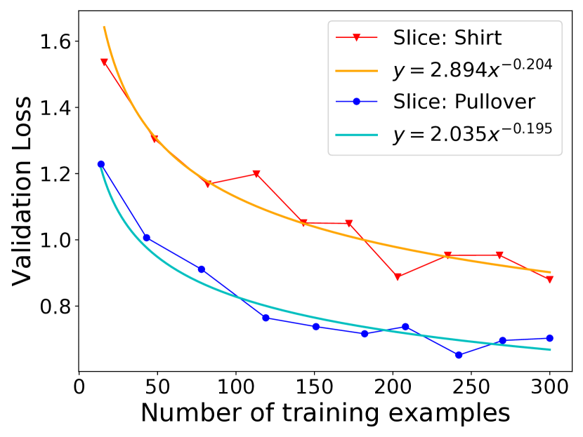
(a) Fashion-MNIST

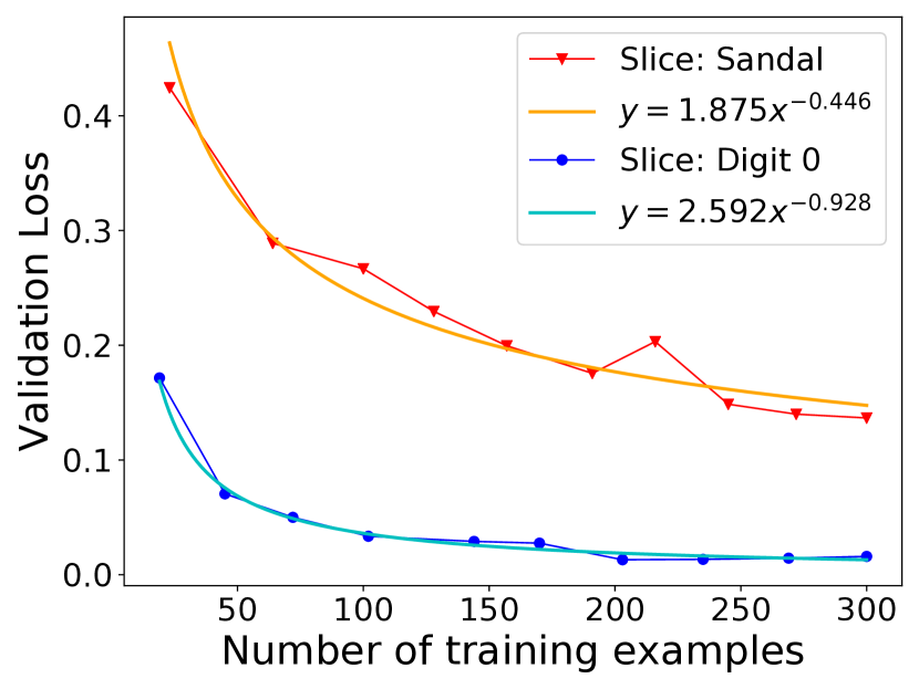
(b) Mixed-MNIST

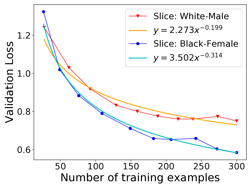
(c) UTKFace

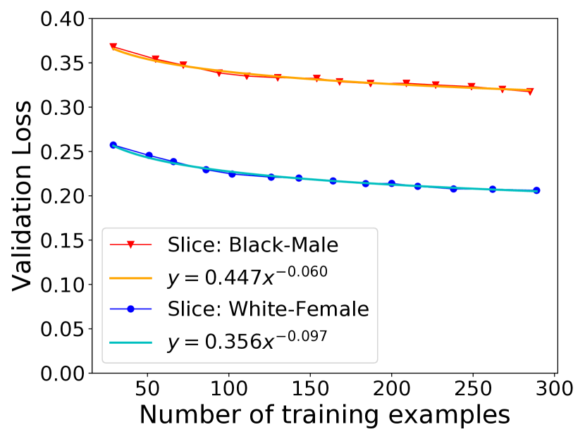
(d) AdultCensus

Figure 8. The learning curves of the four datasets. The initial slice sizes are set to be large enough so we only observe power-law regions without small-data regions. For each dataset, we show two learning curves for different slices fitted using a validation set. Even for seemingly-homogeneous slices in the Fashion-MNIST dataset, the learning curves can be quite different.

We also observe how the learning curve changes as the slice itself grows in size. That is, we increase the slice size and, for each size, fit a new learning curve. Figure 9 shows the learning curves for a slice in the Fashion-MNIST dataset. As a result, the smaller the slice, the more the learning curve deviates from the others. This result shows that the learning curves must be updated as more data is acquired, especially for slices that start small.

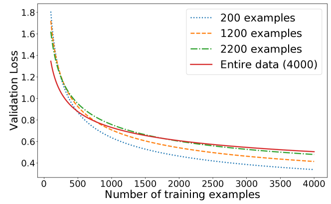
Figure 9. Given a slice in the Fashion-MNIST dataset, we increase its size and train new learning curves. As a result, the learning curves trained on small slices deviate more from the other curves and can be viewed as erroneous.

6.3. Selective Data Acquisition Optimization

We now show the loss and unfairness results of Slice Tuner and make a comparison with the baselines.

6.3.1. Loss and Unfairness of Slice Tuner Methods

Table 2 compares the loss and unfairness results of the Slice Tuner methods on the four datasets. Original is where we train a model on the current slices with no data acquisition. As a result, the Slice Tuner methods improve Original both in terms of loss and unfairness. Among the Slice Tuner methods, the iterative methods outperform One-shot. Between the Aggressive and Conservative methods, Conservative usually has lower loss and unfairness than Aggressive. This result is expected because Conservative uses more iterations to update the learning curves to be more reliable. Finally, Moderate and Aggressive perform similarly, although Moderate has lower loss and unfairness on the Fashion-MNIST dataset.

Dataset	Method	Loss	Avg./Max. EER
Fashion- MNIST	Original	0.423	0.255 / 0.617
	One-shot	0.327	0.174 / 0.542
	Aggressive	0.304	0.144 / 0.351
	Moderate	0.302	0.134 / 0.319
	Conservative	0.300	0.134 / 0.313
Mixed- MNIST	Original	0.299	0.198 / 0.691
	One-shot	0.266	0.181 / 1.169
	Aggressive	0.225	0.119 / 0.395
	Moderate	0.227	0.115 / 0.398
	Conservative	0.223	0.111 / 0.489
UTKFace	Original	0.590	0.097 / 0.207
	One-shot	0.578	0.077 / 0.197
	Aggressive	0.572	0.069 / 0.184
	Moderate	0.572	0.069 / 0.184
	Conservative	0.572	0.069 / 0.184
AdultCensus	Original	0.264	0.104 / 0.168
	One-shot	0.253	0.094 / 0.150
	Aggressive	0.252	0.094 / 0.144
	Moderate	0.252	0.094 / 0.144
	Conservative	0.251	0.093 / 0.144

Table 2. Slice Tuner methods comparison on the 4 datasets.

Dataset	Method	0	1	2	3	4	5	6	7	8	9	# iterations
Fashion-MNIST ($B=6K$)	Original	200	200	200	200	200	200	200	200	200	200	n/a
	One-shot	76	40	761	397	2203	177	1829	268	247	1	1
	Aggressive	888	59	1373	693	1290	40	1400	112	145	0	4
	Moderate	657	45	1336	755	1239	36	1701	96	135	0	4
	Conservative	671	3	1296	599	1495	40	1627	82	173	14	9
Mixed-MNIST ($B=6K$)	Original	150	150	150	150	150	150	150	150	150	150	n/a
	One-shot	33	0	166	47	120	1092	0	637	521	2557	1
	Aggressive	1	16	64	7	163	933	818	597	1202	1552	4
	Moderate	1	0	63	5	99	738	1225	744	989	1500	5
	Conservative	1	2	68	6	133	790	1076	736	1200	1360	10
UTKFace ($B=3K$)	Original	400	400	400	400	400	400	400	400	-	-	n/a
	One-shot	470	427	242	519	448	311	1263	238	-	-	1
	Aggressive	667	384	158	489	560	337	930	365	-	-	2
	Moderate	667	384	158	489	560	337	930	365	-	-	2
	Conservative	667	384	158	489	560	337	930	365	-	-	2
AdultCensus ($B=500$)	Original	150	150	150	150	-	-	-	-	-	-	n/a
	One-shot	0	0	55	445	-	-	-	-	-	-	1
	Aggressive	3	0	164	333	-	-	-	-	-	-	2
	Moderate	3	0	164	333	-	-	-	-	-	-	2
	Conservative	1	0	170	329	-	-	-	-	-	-	3

Table 3. Selective data acquisition results for the experiments in Table 2 where slices are listed numbered from 0 up to 9 (the ordering is not important). For Mixed-MNIST, we select 10 out of the 20 slices. The Original row contains the initial number of examples for each slice while the other rows show the additional number of examples acquired.

Table 3 shows how much data is acquired for each method in Table 2 for the four datasets. For each dataset, the initial slice sizes (same as $L$) are specified in the Original row. While One-shot has only one chance to decide how much data to collect, the Aggressive, Moderate, and Conservative methods have more chances to adjust their results. For example, on the Fashion-MNIST dataset, One-shot overshoots and collects too much data for slices #4 and #6 while the other methods properly adjust their learning curves through more iterations. Another observation is that Conservative uses more iterations than Moderate and Aggressive because it is more conservative in increasing $T$. The exception is UTKFace where all methods perform two iterations. Hence, Conservative can be viewed as trading off efficiency for the lower loss and unfairness results in Table 2.

We also perform the above experiments when the initial slice sizes are not the same and follow an exponential distribution (see Appendix  C). As a result, we make similar observations regarding the Slice Tuner performances.

In summary, the iterative algorithms clearly outperform One-shot. Also, while Moderate and Aggressive have slightly-worse loss and unfairness than Conservative, they use much fewer iterations. Finally, Moderate performs similar to Aggressive overall, but better on Fashion-MNIST. In the following sections, we thus only use Moderate as a representative strategy.

Dataset	$\lambda$	Loss	Avg./Max. EER
Fashion-MNIST	0	0.284	0.160 / 0.402
	0.1	0.285	0.148 / 0.330
	1	0.302	0.129 / 0.330
	10	0.317	0.112 / 0.217
Mixed-MNIST	0	0.208	0.136 / 0.582
	0.1	0.212	0.134 / 0.444
	1	0.219	0.120 / 0.462
	10	0.224	0.116 / 0.468
UTKFace	0	0.637	0.077 / 0.159
	0.1	0.639	0.076 / 0.144
	1	0.651	0.065 / 0.160
	10	0.651	0.058 / 0.148
AdultCensus	0	0.246	0.104 / 0.170
	0.1	0.247	0.105 / 0.168
	1	0.248	0.104 / 0.166
	10	0.248	0.104 / 0.165

Table 4. Results of Moderate when varying $\lambda$.

Method	0	1	2	3	4	5	6	7	8	9
Original	200	200	200	200	200	200	200	200	200	200
$\lambda=0$	755	171	880	606	1028	312	1196	402	366	284
$\lambda=0.1$	921	233	969	504	963	247	1304	363	199	297
$\lambda=1$	915	33	1301	447	1451	19	1677	56	92	9
$\lambda=10$	969	0	1170	277	1541	0	2043	0	0	0

Table 5. Selective data acquisition results for the Fashion-MNIST experiments in Table 4.

6.3.2. Balancing $\lambda$

We study the effect of balancing $\lambda$. Recall that a higher $\lambda$ means there is more emphasis on optimizing fairness. How to set $\lambda$ depends on whether the loss or unfairness is more important to minimize for the given application. Table 4 shows the loss and unfairness results on the four datasets when varying $\lambda$ using the Moderate method and the same initial data and budget as in Table 3. As $\lambda$ increases, the avg. and max. EER results decrease while the loss increases.

Table 5 shows the amounts of data acquired per slice for different $\lambda$ values using the Fashion-MNIST dataset. The results for the other datasets (not shown) are similar. In our example, slices #2, #4, and #6 start with higher losses than other slices, and the experiments with higher $\lambda$ values results tend to be more aggressive in acquiring data for those three slices in order to reduce the unfairness.

Dataset	Measure	Alg.	Basic		Bad for Uniform		Bad for Water filling
			Initial	3000	Initial	3000	Initial	3000
	Loss	Uni	0.472 $\pm$ 0.002	0.355 $\pm$ 0.003	0.445 $\pm$ 0.003	0.334 $\pm$ 0.002	0.426 $\pm$ 0.002	0.322 $\pm$ 0.003
	(# Iters)	WF		0.355 $\pm$ 0.003		0.323 $\pm$ 0.002		0.330 $\pm$ 0.003
Fashion-		Mod		0.341 $\pm$ 0.002 (3)		0.314 $\pm$ 0.002 (2)		0.318 $\pm$ 0.002 (3)
MNIST	Avg. EER	Uni	0.283 $\pm$ 0.006	0.230 $\pm$ 0.004	0.308 $\pm$ 0.009	0.226 $\pm$ 0.007	0.210 $\pm$ 0.004	0.177 $\pm$ 0.003
		WF		0.230 $\pm$ 0.004		0.217 $\pm$ 0.005		0.200 $\pm$ 0.003
		Mod		0.173 $\pm$ 0.006		0.168 $\pm$ 0.003		0.157 $\pm$ 0.002
	Loss	Uni	0.301 $\pm$ 0.003	0.240 $\pm$ 0.002	0.264 $\pm$ 0.003	0.229 $\pm$ 0.002	0.266 $\pm$ 0.002	0.226 $\pm$ 0.002
	(# Iters)	WF		0.240 $\pm$ 0.002		0.221 $\pm$ 0.002		0.228 $\pm$ 0.001
Mixed-		Mod		0.235 $\pm$ 0.001 (3)		0.216 $\pm$ 0.002 (2)		0.219 $\pm$ 0.002 (3)
MNIST	Avg. EER	Uni	0.207 $\pm$ 0.004	0.182 $\pm$ 0.002	0.205 $\pm$ 0.004	0.182 $\pm$ 0.002	0.166 $\pm$ 0.003	0.157 $\pm$ 0.003
		WF		0.182 $\pm$ 0.002		0.166 $\pm$ 0.002		0.167 $\pm$ 0.002
		Mod		0.147 $\pm$ 0.002		0.146 $\pm$ 0.002		0.133 $\pm$ 0.003
UTKFace	Loss	Uni	0.562 $\pm$ 0.003	0.554 $\pm$ 0.005	0.611 $\pm$ 0.005	0.579 $\pm$ 0.003	0.597 $\pm$ 0.004	0.575 $\pm$ 0.004
	(# Iters)	WF		0.554 $\pm$ 0.005		0.573 $\pm$ 0.004		0.577 $\pm$ 0.003
		Mod		0.547 $\pm$ 0.004 (1)		0.571 $\pm$ 0.004 (1)		0.569 $\pm$ 0.003 (1)
	Avg. EER	Uni	0.091 $\pm$ 0.005	0.081 $\pm$ 0.009	0.117 $\pm$ 0.006	0.095 $\pm$ 0.004	0.093 $\pm$ 0.007	0.087 $\pm$ 0.006
		WF		0.081 $\pm$ 0.009		0.090 $\pm$ 0.004		0.074 $\pm$ 0.005
		Mod		0.071 $\pm$ 0.005		0.078 $\pm$ 0.005		0.072 $\pm$ 0.004
			Initial	300	Initial	300	Initial	300
AdultCensus	Loss	Uni	0.263 $\pm$ 0.001	0.257 $\pm$ 0.001	0.258 $\pm$ 0.001	0.254 $\pm$ 0.001	0.287 $\pm$ 0.001	0.286 $\pm$ 0.001
	(# Iters)	WF		0.257 $\pm$ 0.001		0.247 $\pm$ 0.000		0.288 $\pm$ 0.001
		Mod		0.253 $\pm$ 0.001 (1)		0.245 $\pm$ 0.000 (1)		0.284 $\pm$ 0.001 (2)
	Avg. EER	Uni	0.103 $\pm$ 0.001	0.099 $\pm$ 0.000	0.109 $\pm$ 0.001	0.106 $\pm$ 0.000	0.137 $\pm$ 0.001	0.137 $\pm$ 0.002
		WF		0.099 $\pm$ 0.000		0.101 $\pm$ 0.000		0.137 $\pm$ 0.001
		Mod		0.094 $\pm$ 0.000		0.100 $\pm$ 0.000		0.134 $\pm$ 0.001

Table 6. A detailed comparison of Moderate(Mod) against the two baselines – Uniform(Uni) and Water filling(WF) – on the four datasets where we use three settings and vary the budget $B$. We also set $\lambda=0.1$.

6.3.3. Comparison with Baselines

We make a detailed comparison between Moderate and the baselines Uniform and Water filling in Table 6 where we use three settings: (1) a basic setting where slices have the same amounts of data, (2) a pathological setting for Uniform (called “Bad for Uniform”) where there are many slices with low loss, and (3) a pathological setting for Water filling (called “Bad for Water filling”) where there is a large slice with high loss and a small slice with low loss. For each setting, we compare the three methods using a budget of $B$ = 3K except for the AdultCensus dataset where $B$ = 300 is already enough to obtain low loss. As a result, Moderate has both lower loss and avg. EER than the baselines for all datasets. Looking at the two baselines, Uniform performs worse than Water filling in setting (2) while Water filling performs worse in setting (3). For all experiments, Moderate mostly performs 1–3 iterations as shown in the parentheses in Table 6.

Figure 10 shows a more detailed comparison with the baselines using the basic setting above (i.e., setting (1)) and the Mixed-MNIST dataset. Here the two baselines happen to have the same loss and unfairness results. For varying budgets, Moderate clearly outperforms the two baselines in terms of loss and unfairness. Although the improvements in loss are not as drastic as those in unfairness, they are still significant: in order to obtain the same losses, the baselines need to increase their budgets by 15–100%.

We also perform the experiments with ResNet-18 (He et al., 2016) (one of the state-of-the-art models for image classification) using the basic setting and the Fashion-MNIST dataset. The results are in Appendix  B, and the trends are similar to Table 6 where Moderate outperforms the baselines in terms of loss and unfairness.

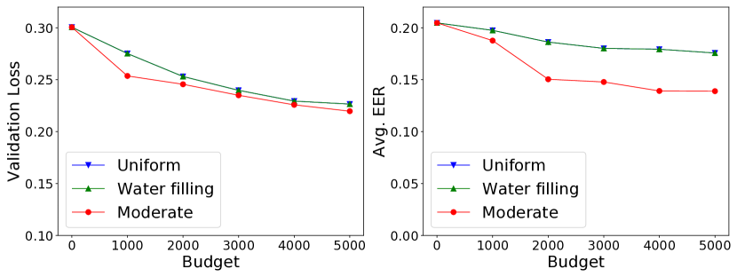
Figure 10. Loss and unfairness comparison (Mixed-MNIST).

6.3.4. Unreliable learning curves

Learning curves are not always “perfect” in the sense that they cleanly follow a power law. For example, if the slice size is small, then the learning curve is more likely to be noisy. Even if the slice size is not small, some slices may still exhibit noisy learning curves for other reasons.

In this section, we consider the scenario of small slices where we lower the initial slice sizes of the Fashion-MNIST dataset to $L=30$ where the learning curves are noisy and unreliable as shown in Figure 11. Nonetheless, Table 7 shows that Slice Tuner still performs better than the baselines because it can leverage the relative differences (loss and steepness) of the learning curves. Even if the learning curves are completely useless, Slice Tuner’s performance should fall back to those of the baselines. In a sense, the learning curves are used as hints and do not have to be perfect. However, as more data is acquired, the learning curves will gradually become more reliable and informative.

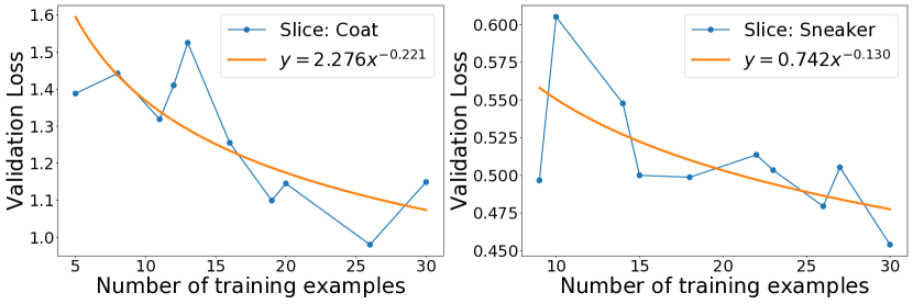
Figure 11. Learning curves are noisy for small slices of Fashion-MNIST.

Init. Size	Method	Loss	Avg. / Max. EER
	Original	0.583	0.317 / 0.792
30	Uniform	0.508	0.302 / 0.786
($B=500$)	Water filling	0.508	0.302 / 0.786
	Moderate	0.475	0.259 / 0.650

Table 7. Loss and unfairness results of Slice Tuner methods for the small slice sizes of Fashion-MNIST.

6.4. Efficient Learning Curve Generation

We evaluate the efficient learning curve generation method described in Section 4.2 as shown in Table 8. The default Moderate method uses the efficient learning curve generation. We make a comparison with a modified version of Moderate where the learning curve generation is done exhaustively (called “Exhaustive”). We also vary the initial slice size and budget. As a result, Moderate is 11-12x faster than Exhaustive as expected and obtains slightly worse or even better loss and unfairness results. While it may sound counter intuitive that Moderate can have lower loss and unfairness, this may happen because our optimization of taking X% examples of all slices together has the effect of removing bias among the slices. The reason the runtime speedups are larger than the number of slices (10) is that the model training itself is on average faster because it is performed on smaller data as explained in Section 4.2. We consider the runtimes of Moderate to be practical because the main bottleneck of Slice Tuner is the time to actually acquire data, which may take say hours.

Method	Loss	Avg. / Max. EER	Runtime (sec)
Init. size = 200, $B$ = 2K
Exhaustive	0.351	0.159 / 0.388	20,275
Slice Tuner	0.346	0.164 / 0.362	1,847
Init. size = 300, $B$ = 3K
Exhaustive	0.301	0.138 / 0.375	24,673
Slice Tuner	0.303	0.137 / 0.303	2,088

Table 8. A comparison between exhaustively generating learning curves versus the Moderate method on Fashion-MNIST for different initial slice sizes and budget values.

7. Related Work

Data Acquisition

Acquiring data is becoming increasingly convenient. Dataset searching (Nargesian et al., 2019) focuses on finding the right datasets either on the Web or within a data lake. As a recent example, Google Dataset Search (Benjelloun et al., 2020) started its service in 2016 with 500K public science datasets, but now has 30M datasets. Another traditional approach is crowdsourcing (ama, [n.d.]), where one can hire workers to generate new data. Yet another interesting branch of research is to use simulators (Kim et al., 2019) to generate infinite numbers of realistic examples. Slice Tuner complements these systems by determining how much data to acquire per slice based on a given ML model.

Although the notion of selective data acquisition seems relevant to active learning (Settles, 2012), they solve different problems. While active learning selects which existing unlabeled data to label, Slice Tuner decides how much non-existing data to acquire per slice. Hence, the active learning techniques do not apply for data acquisition.

The closest work to Slice Tuner is reference (Chen et al., 2018), which also acquires data to improve model accuracy and fairness. A key observation is that unfairness can be decomposed into bias, variance, and noise, and that data acquisition can reduce unfairness without sacrificing accuracy. Similar to Slice Tuner, reference (Chen et al., 2018) assumes that learning curves follow a power law. However, the learning curves are primarily used to improve fairness, and the data acquisition method is simplistic where the amounts of data acquired follow the original data distribution. In comparison, Slice Tuner takes the more sophisticated approach of using learning curves to optimize both accuracy and fairness and addresses the challenge of unreliable learning curves using efficient iterative updates.

Another close work (Asudeh et al., 2019) performs data acquisition such that all possible slices are large enough. This problem is analogous to Water filling (Figure 3(b)) where the slices are guaranteed a minimal data coverage, but in the more challenging setting where slices may overlap with each other, and there is a combinatorial explosion in the number of slices. In comparison, Slice Tuner assumes the slices partition the entire dataset and selectively acquires data to improve accuracy and fairness instead of achieving minimum coverage.

Multi-armed Bandit

Slice Tuner can be viewed as solving a specialized multi-armed bandit problem (Auer et al., 2002). Among the known variants, rotting bandit (RB)  (Levine et al., 2017) is the most relevant where each arm’s expected reward decays as a function of the pulls of that arm, which corresponds to the diminishing benefit of newly-acquired data in our setting. However, there is no fairness notion of ensuring the rewards across slots are similar in RB. Moreover, RB only uses prior knowledge on the rotting models, but we use prior knowledge on the reward models including rotting, which we capture as power-law learning curves. Our prior knowledge is not strong because learning curves may change as we acquire data, but can be used to select multiple slots that together minimize loss and unfairness. Finally, RB assumes independent arms while we assume dependence where pulling one arm may change the expected rewards of others.

Model Fairness

As ML is used more broadly, model fairness is becoming a critical issue (Venkatasubramanian, 2019). Fairness is a subjective notion, so there is no universally-agreed definition. Some standard definitions include demographic parity (Feldman et al., 2015), equalized odds (Hardt et al., 2016), equal opportunity (Hardt et al., 2016), and equalized error rates (Venkatasubramanian, 2019; Zafar et al., 2017). Other popular notions of fairness include individual fairness (Dwork et al., 2012) and causality-based fairness (Kilbertus et al., 2017). Among them, we choose equalized error rates because it is relevant to ML systems that must provide similar-quality services to users. In addition, equalized error rates is a familiar concept in the systems literature where the system performance must be uniform across data partitions.

Model Analysis and Learning Curves

An ML model should be viewed as software and thus needs to be analyzed and debugged as well. Industrial tools like TensorFlow Model Analysis (tfm, [n.d.]) provide visualizations of model accuracy per slice. More recently, automatic data slicing techniques (Chung et al., 2019) have been proposed to find underperforming slices. Estimating learning curves has been mainly studied in the computer vision community (Hestness et al., 2017; Cho et al., 2015; Figueroa et al., 2012; Hajian-Tilaki, 2014). Baidu (Hestness et al., 2017) analyzes four ML domains of how the learning curve changes depending on the amount of data and observes a power-law error scaling. This result is further supported theoretically (AMA, 1993) and empirically (Domhan et al., 2015). Reference (Chen et al., 2018) also utilizes a power-law learning curve to acquire data and improve fairness.

8. Conclusion

We proposed Slice Tuner, which performs selective data acquisition to optimize model accuracy and fairness. Slice Tuner estimates learning curves for different slices and solving an optimization problem to determine how much data acquisition is needed for each slice given a budget. To address the challenges of unreliable learning curves and dependencies among slices, we proposed iterative algorithms that repeatedly update the learning curves as more data is acquired, using the imbalance ratio change as a proxy to estimate influence. We demonstrated on real datasets that our iterative algorithms are efficient and obtain lower loss and unfairness than the two baseline methods that do not exploit the learning curves, even if the learning curves are unreliable. In addition, we demonstrated the practicality of Slice Tuner by acquiring new data using Amazon Mechanical Turk. In the future, we would like to improve our influence estimation and support overlapping slices.

Acknowledgments

This work was supported by a Google AI Focused Research Award and by the National Research Foundation of Korea(NRF) grant funded by the Korea government(MSIT) (No. NRF-2018R1A5A1059921 and NRF-2021R1C1C1005999).

Appendix A Data slicing

In this section, we briefly discuss various approaches for data slicing. While this topic is not the main focus of this paper, it is worth discussing the state-of-the-art methods. The straightforward way is to select slices manually based on domain knowledge. For example, for a movie recommendation system, one may select slices based on genre. Alternatively, one can determine slices based on model analysis. Manual tools for visualization (tfm, [n.d.]; Kahng et al., 2016) can be used to find problematic slices where a model underperforms. Recently, there are automatic tools (Chung et al., 2019) that can find such slices.

As we mentioned in Section 2.1, a desirable property of a slice is to be unbiased so that the acquired examples have similar effects on the model accuracy. Using large slices that are biased is undesirable. For example, a slice that contains all regions of Figure 1(a) is bad because there is a bias towards American customers. That is, adding an American customer example is not as helpful as say adding a European customer example. On the other hand, using slices that are not biased, but too small is also problematic because we may need to maintain many learning curves that are not accurate due to the small amounts of data.

In order to find the largest-possible slices that are still unbiased, one can use a method similar to decision tree training where the goal is to find partitions of the data such that the impurity (i.e., homogeneity of labels in leaf nodes) is minimized. Instead of minimizing impurity, we would have to compute the bias in slices using say an entropy-based measure. Starting from the entire dataset, we can iteratively split slices that have biases in their data for different values of attributes. The splitting can terminate once the average entropy is above some threshold.

Appendix B ResNet-18 Results on Fashion-MNIST

In Section  6, we used basic convolution neural networks and single fully connected layers for all experiments. In this section, we performed the same experiments with ResNet-18 (He et al., 2016) (one of the state-of-the-art models for image classification) using the basic setting and Fashion-MNIST dataset. In Table 9, the key trends are still similar to Table 6 where Moderate outperforms baselines in terms of loss and fairness. Compared to the Fashion-MNIST results in Table 6, the losses actually increase because ResNet-18’s architecture is overly complex to train on the modest-sized Fashion-MNIST dataset.

Init. Size	Method	Loss	Avg. / Max. EER
	Original	0.567	0.240 / 0.481
400	Uniform	0.484	0.228 / 0.452
($B=3K$)	Water filling	0.484	0.228 / 0.452
	Moderate	0.480	0.190 / 0.422

Table 9. Loss and unfairness results of Slice Tuner methods for the ResNet-18 on Fashion-MNIST.

Appendix C Exponential Distribution Results

In Section 6.3.1, we evaluated the Slice Tuner methods when the initial slice sizes are the same. In this section, we perform the same experiments when the initial slice sizes follow an exponential distribution. In Table 10, the key trends are similar to Table 2 where iterative algorithms outperform One-shot because One-shot tends to acquire too much data for certain slices as shown in Table 11. Moreover, while Conservative uses more iterations than Aggressive and Moderate, it has slightly-better loss and unfairness results.

Dataset	Method	Loss	Avg./Max. EER
Fashion- MNIST	Original	0.455	0.260 / 0.911
	One-shot	0.349	0.178 / 0.448
	Aggressive	0.312	0.116 / 0.232
	Moderate	0.308	0.125 / 0.306
	Conservative	0.307	0.116 / 0.299
Mixed- MNIST	Original	0.292	0.200 / 0.903
	One-shot	0.249	0.157 / 0.934
	Aggressive	0.231	0.124 / 0.465
	Moderate	0.231	0.124 / 0.465
	Conservative	0.223	0.117 / 0.381
UTKFace	Original	0.710	0.170 / 0.369
	One-shot	0.655	0.114 / 0.285
	Aggressive	0.638	0.114 / 0.285
	Moderate	0.638	0.114 / 0.285
	Conservative	0.638	0.114 / 0.285
AdultCensus	Original	0.274	0.107 / 0.172
	One-shot	0.253	0.095 / 0.150
	Aggressive	0.252	0.095 / 0.149
	Moderate	0.252	0.095 / 0.149
	Conservative	0.252	0.095 / 0.149

Table 10. Slice Tuner methods comparison on the 4 datasets where the initial slice sizes follow an exponential distribution as shown in Table 11.

Dataset	Method	0	1	2	3	4	5	6	7	8	9	# iterations
Fashion-MNIST ($B=6K$)	Original	400	282	230	200	178	163	151	141	133	126	n/a
	One-shot	0	0	596	192	1495	201	3019	371	128	0	1
	Aggressive	434	24	1406	348	1299	77	2136	88	188	0	4
	Moderate	373	74	1602	1737	396	617	61	558	965	42	5
	Conservative	727	51	1666	1604	641	780	47	951	790	79	9
Mixed-MNIST ($B=6K$)	Original	600	346	268	200	189	180	166	160	154	145	n/a
	One-shot	0	0	0	176	61	0	1457	673	1136	2008	1
	Aggressive	0	0	0	57	32	1432	946	653	1309	1356	3
	Moderate	0	0	0	57	32	1432	946	653	1309	1356	3
	Conservative	0	0	0	90	59	800	936	730	1240	1562	6
UTKFace ($B=3K$)	Original	400	263	206	174	152	136	124	114	-	-	n/a
	One-shot	23	123	245	315	322	279	745	276	-	-	1
	Aggressive	90	138	146	308	367	296	574	378	-	-	2
	Moderate	90	138	146	308	367	296	574	378	-	-	2
	Conservative	90	138	146	308	367	296	574	378	-	-	2
AdultCensus ($B=500$)	Original	150	106	86	75	-	-	-	-	-	-	n/a
	One-shot	0	0	425	75	-	-	-	-	-	-	1
	Aggressive	0	0	232	268	-	-	-	-	-	-	2
	Moderate	0	0	232	268	-	-	-	-	-	-	2
	Conservative	0	0	232	268	-	-	-	-	-	-	2

Table 11. Selective data acquisition results for the experiments in Table 10 where slices are listed numbered from 0 up to 9 (the ordering is not important), and their initial sizes follow an exponential distribution. For Mixed-MINST, we select 10 out of 20 slices. The Original row contains the initial number of examples for each slice while the other rows show the additional number of examples acquired.

References

- (1)
- ama ([n.d.]) [n.d.]. Amazon Mechanical Turk. https://www.mturk.com/.
- git ([n.d.]) [n.d.]. Slice Tuner Github repository. https://github.com/systemT2021/SliceTuner.
- kar ([n.d.]) [n.d.]. Software 2.0. https://medium.com/@karpathy/software-2-0-a64152b37c35.
- tfm ([n.d.]) [n.d.]. TensorFlow Model Analysis. https://github.com/tensorflow/model-analysis.
- AMA (1993) 1993. A universal theorem on learning curves. Neural Networks 6, 2 (1993), 161 – 166.
- Abadi et al. (2016) Martín Abadi, Paul Barham, Jianmin Chen, Zhifeng Chen, Andy Davis, Jeffrey Dean, Matthieu Devin, Sanjay Ghemawat, Geoffrey Irving, Michael Isard, Manjunath Kudlur, Josh Levenberg, Rajat Monga, Sherry Moore, Derek Gordon Murray, Benoit Steiner, Paul A. Tucker, Vijay Vasudevan, Pete Warden, Martin Wicke, Yuan Yu, and Xiaoqiang Zheng. 2016. TensorFlow: A System for Large-Scale Machine Learning. In OSDI. 265–283.
- Asudeh et al. (2019) Abolfazl Asudeh, Zhongjun Jin, and H. V. Jagadish. 2019. Assessing and Remedying Coverage for a Given Dataset. ICDE (2019), 554–565.
- Auer et al. (2002) Peter Auer, Nicolò Cesa-Bianchi, and Paul Fischer. 2002. Finite-Time Analysis of the Multiarmed Bandit Problem. 47, 2–3 (2002), 235–256.
- Baylor et al. (2017) Denis Baylor, Eric Breck, Heng-Tze Cheng, Noah Fiedel, Chuan Yu Foo, Zakaria Haque, Salem Haykal, Mustafa Ispir, Vihan Jain, Levent Koc, et al. 2017. TFX: A TensorFlow-Based Production-Scale Machine Learning Platform. In KDD. 1387–1395.
- Benjelloun et al. (2020) Omar Benjelloun, Shiyu Chen, and Natasha F. Noy. 2020. Google Dataset Search by the Numbers. CoRR abs/2006.06894 (2020). arXiv:2006.06894
- Buda et al. (2018) Mateusz Buda, Atsuto Maki, and Maciej A. Mazurowski. 2018. A systematic study of the class imbalance problem in convolutional neural networks. Neural Networks 106 (2018), 249 – 259.
- Chen et al. (2018) Irene Y. Chen, Fredrik D. Johansson, and David A. Sontag. 2018. Why Is My Classifier Discriminatory?. In NeurIPS. 3543–3554.
- Cho et al. (2015) Junghwan Cho, Kyewook Lee, Ellie Shin, Garry Choy, and Synho Do. 2015. Medical Image Deep Learning with Hospital PACS Dataset. CoRR abs/1511.06348 (2015). arXiv:1511.06348
- Chung et al. (2019) Yeounoh Chung, Tim Kraska, Neoklis Polyzotis, Ki Hyun Tae, and Steven Euijong Whang. 2019. Slice Finder: Automated Data Slicing for Model Validation. IEEE TKDE (2019).
- Domhan et al. (2015) Tobias Domhan, Jost Tobias Springenberg, and Frank Hutter. 2015. Speeding Up Automatic Hyperparameter Optimization of Deep Neural Networks by Extrapolation of Learning Curves. In IJCAI. 3460–3468.
- Dwork et al. (2012) Cynthia Dwork, Moritz Hardt, Toniann Pitassi, Omer Reingold, and Richard Zemel. 2012. Fairness Through Awareness. In ITCS (Cambridge, Massachusetts). ACM, New York, NY, USA, 214–226.
- Feldman et al. (2015) Michael Feldman, Sorelle A. Friedler, John Moeller, Carlos Scheidegger, and Suresh Venkatasubramanian. 2015. Certifying and Removing Disparate Impact. In KDD. 259–268.
- Figueroa et al. (2012) Rosa L. Figueroa, Qing Zeng-Treitler, Sasikiran Kandula, and Long H. Ngo. 2012. Predicting sample size required for classification performance. BMC Med. Inf. & Decision Making 12 (2012), 8.
- Hajian-Tilaki (2014) Karimollah Hajian-Tilaki. 2014. Sample size estimation in diagnostic test studies of biomedical informatics. Journal of Biomedical Informatics 48 (2014), 193–204.
- Hardt et al. (2016) Moritz Hardt, Eric Price, and Nati Srebro. 2016. Equality of Opportunity in Supervised Learning. In NeurIPS. 3315–3323.
- He et al. (2016) K. He, X. Zhang, S. Ren, and J. Sun. 2016. Deep Residual Learning for Image Recognition. In CVPR. 770–778.
- Hestness et al. (2017) Joel Hestness, Sharan Narang, Newsha Ardalani, Gregory F. Diamos, Heewoo Jun, Hassan Kianinejad, Md. Mostofa Ali Patwary, Yang Yang, and Yanqi Zhou. 2017. Deep Learning Scaling is Predictable, Empirically. CoRR abs/1712.00409 (2017).
- Kahng et al. (2016) Minsuk Kahng, Dezhi Fang, and Duen Horng Polo Chau. 2016. Visual exploration of machine learning results using data cube analysis. In HILDA. ACM, 1.
- Kilbertus et al. (2017) Niki Kilbertus, Mateo Rojas-Carulla, Giambattista Parascandolo, Moritz Hardt, Dominik Janzing, and Bernhard Schölkopf. 2017. Avoiding Discrimination through Causal Reasoning. In NeurIPS. 656–666.
- Kim et al. (2019) Hoon Kim, Kangwook Lee, Gyeongjo Hwang, and Changho Suh. 2019. Crash to Not Crash: Learn to Identify Dangerous Vehicles Using a Simulator. In AAAI. 978–985.
- Kohavi (1996) Ron Kohavi. 1996. Scaling Up the Accuracy of Naive-Bayes Classifiers: A Decision-Tree Hybrid. In KDD. 202–207.
- LeCun et al. (2001) Y. LeCun, L. Bottou, Y. Bengio, and P. Haffner. 2001. Gradient-Based Learning Applied to Document Recognition. In Intelligent Signal Processing. IEEE Press, 306–351.
- Levine et al. (2017) Nir Levine, Koby Crammer, and Shie Mannor. 2017. Rotting Bandits. In Advances in Neural Information Processing Systems 30. Curran Associates, Inc., 3074–3083.
- Nargesian et al. (2019) Fatemeh Nargesian, Erkang Zhu, Renée J. Miller, Ken Q. Pu, and Patricia C. Arocena. 2019. Data Lake Management: Challenges and Opportunities. Proc. VLDB Endow. 12, 12 (2019), 1986–1989.
- Polyzotis et al. (2018) Neoklis Polyzotis, Sudip Roy, Steven Euijong Whang, and Martin Zinkevich. 2018. Data Lifecycle Challenges in Production Machine Learning: A Survey. SIGMOD Record 47, 2 (2018), 17–28.
- Proakis (2007) Proakis. 2007. Digital Communications 5th Edition. McGraw Hill.
- Ratner et al. (2019) Alexander J. Ratner, Braden Hancock, and Christopher Ré. 2019. The Role of Massively Multi-Task and Weak Supervision in Software 2.0. In CIDR.
- Roh et al. (2019) Yuji Roh, Geon Heo, and Steven Euijong Whang. 2019. A Survey on Data Collection for Machine Learning: a Big Data - AI Integration Perspective. IEEE Trans. Knowl. Data Eng. (2019).
- Settles (2012) Burr Settles. 2012. Active Learning. Morgan & Claypool Publishers.
- Sheng et al. (2008) Victor S. Sheng, Foster J. Provost, and Panagiotis G. Ipeirotis. 2008. Get another label? improving data quality and data mining using multiple, noisy labelers. In KDD. 614–622.
- Venkatasubramanian (2019) Suresh Venkatasubramanian. 2019. Algorithmic Fairness: Measures, Methods and Representations. In PODS. 481.
- Xiao et al. (2017) Han Xiao, Kashif Rasul, and Roland Vollgraf. 2017. Fashion-MNIST: a Novel Image Dataset for Benchmarking Machine Learning Algorithms. arXiv:cs.LG/1708.07747 [cs.LG]
- Zafar et al. (2017) Muhammad Bilal Zafar, Isabel Valera, Manuel Gomez-Rodriguez, and Krishna P. Gummadi. 2017. Fairness Beyond Disparate Treatment & Disparate Impact: Learning Classification without Disparate Mistreatment. In WWW. 1171–1180.
- Zaharia et al. (2018) Matei Zaharia, Andrew Chen, Aaron Davidson, Ali Ghodsi, Sue Ann Hong, Andy Konwinski, Siddharth Murching, Tomas Nykodym, Paul Ogilvie, Mani Parkhe, Fen Xie, and Corey Zumar. 2018. Accelerating the Machine Learning Lifecycle with MLflow. IEEE Data Eng. Bull. 41, 4 (2018), 39–45.
- Zhang et al. (2017) Zhifei Zhang, Yang Song, and Hairong Qi. 2017. Age Progression/Regression by Conditional Adversarial Autoencoder. In CVPR.