PUTP-2614

Loop Equation and Exact Soft Anomalous Dimension
in 𝒩=4𝒩4\mathcal{N}=4 Super Yang-Mills

Simone Giombi, Shota Komatsu

Department of Physics, Princeton University, Princeton, NJ 08544, USA
School of Natural Sciences, Institute for Advanced Study, Princeton, NJ 08540, USA

sgiombi AT princeton.edu, skomatsu AT ias.edu

Abstract

BPS Wilson loops in supersymmetric gauge theories have been the subjects of active research since they are often amenable to exact computation. So far most of the studies have focused on loops that do not intersect. In this paper, we derive exact results for intersecting 1/8181/8 BPS Wilson loops in 𝒩=4𝒩4\mathcal{N}=4 supersymmetric Yang-Mills theory, using a combination of supersymmetric localization and the loop equation in 2d gauge theory. The result is given by a novel matrix-model-like representation which couples multiple contour integrals and a Gaussian matrix model. We evaluate the integral at large N𝑁N, and make contact with the string worldsheet description at strong coupling. As an application of our results, we compute exactly a small-angle limit (and more generally near-BPS limits) of the cross anomalous dimension which governs the UV divergence of intersecting Wilson lines. The same quantity describes the soft anomalous dimension of scattering amplitudes of W𝑊W-bosons in the Coulomb branch.

1 Introduction

The loop equation was proposed initially in [1, 2] as an alternative way to formulate, and possibly solve, the gauge theories (see e.g. [3] for a review). It has the conceptual advantage that it directly constrains the most basic observables, namely the Wilson loops. In lower-dimensional theories such as matrix models [4] and two-dimensional Yang-Mills theory [5, 6, 7, 8, 9], it has proven to be a powerful tool for solving the theories exactly. Unfortunately, solving the loop equation is much harder in higher dimensions and progress remains to be made.

In this paper we demonstrate the power of the loop equation in higher dimensions when used in conjunction with other non-perturbative techniques. Specifically, we consider intersecting 1/8181/8-BPS Wilson loops in 𝒩=4𝒩4\mathcal{N}=4 supersymmetric Yang-Mills (𝒩=4𝒩4\mathcal{N}=4 SYM) and compute their expectation values at finite coupling and finite N𝑁N using a combination of the loop equation and supersymmetric localization [10, 11].

The 1/8181/8-BPS Wilson loop is a supersymmetric Wilson loops in 𝒩=4𝒩4\mathcal{N}=4 SYM which can be defined on a arbitrary contour on a two-sphere and preserves four fermionic charges. It was conjectured in [12, 13] and later supported by supersymmetric localization [11] that its expectation value (as well as general correlation functions of any number of loops) conicides with that of the standard Wilson loop in two-dimensional Yang-Mills theory (2d YM) in a zero-instanton sector. Based on this, the expectation value of a non-intersecting 1/8181/8-BPS loop was computed in [12, 13] generalizing the famous result for the 1/2121/2-BPS loop [14, 15, 10]. It was also used to derive multi-matrix models for correlators of local operators and non-intersecting BPS loops[16, 17]. By now these results have been tested by numerous direct computations [18, 19, 20, 21, 22, 23] and they provide convincing evidence for the equivalence between the BPS sector of 𝒩=4𝒩4\mathcal{N}=4 SYM and 2d YM.

The goal of this paper is to generalize them to intersecting loops. The strategy is simple: Using the conjecture above, we relate the intersecting 1/8181/8-BPS loops in 𝒩=4𝒩4\mathcal{N}=4 SYM to intersecting Wilson loops in 2d YM on S2superscript𝑆2S^{2} in the zero-instanton sector. We then solve the loop equation of 2d YM exactly at finite N𝑁N. The loop equation in 2d YM was first solved for loops on R2superscript𝑅2R^{2} at large N𝑁N [5]. The result was generalized to loops on R2superscript𝑅2R^{2} at finite N𝑁N in [6] and to loops on S2superscript𝑆2S^{2} at large N𝑁N in [7, 8, 9]. While all these results take simple and compact forms, no such expressions were known for loops on S2superscript𝑆2S^{2} at finite N𝑁N: the only known expression in the literature involves a rather complicated sum over the Young diagrams [24]. We show that a simple closed-form expression does exist for loops on S2superscript𝑆2S^{2} at finite N𝑁N if the theory is restricted to the zero-instanton sector—the sector relevant for the BPS loops in 𝒩=4𝒩4\mathcal{N}=4 SYM.

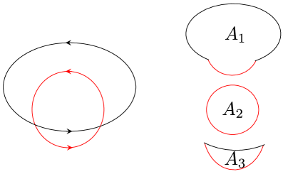
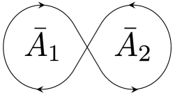
The result of our computation is a coupled system of multiple integrals and a Gaussian matrix model. For instance, the expectation value of the figure eight loop with areas A¯1subscript¯𝐴1\bar{A}_{1} and A¯2subscript¯𝐴2\bar{A}_{2} reads (see figure 1)

𝒲figure-eight=iπλ𝒞1𝒞2𝑑u1𝑑u2u1u2(u1u2)2+(λ4πN)2f4πA¯1(u1)fA¯2(u2)M.delimited-⟨⟩subscript𝒲figure-eight𝑖𝜋𝜆subscriptcontour-integralprecedessubscript𝒞1subscript𝒞2differential-dsubscript𝑢1differential-dsubscript𝑢2subscript𝑢1subscript𝑢2superscriptsubscript𝑢1subscript𝑢22superscript𝜆4𝜋𝑁2subscriptdelimited-⟨⟩subscript𝑓4𝜋subscript¯𝐴1subscript𝑢1subscript𝑓subscript¯𝐴2subscript𝑢2𝑀\langle\mathcal{W}_{\text{figure-eight}}\rangle=\frac{i}{\pi\lambda}\oint_{\mathcal{C}_{1}\prec\mathcal{C}_{2}}du_{1}du_{2}\frac{u_{1}-u_{2}}{(u_{1}-u_{2})^{2}+\left(\frac{\lambda}{4\pi N}\right)^{2}}\left<f_{4\pi-\bar{A}_{1}}(u_{1})f_{\bar{A}_{2}}(u_{2})\right>_{M}\,. (1.1)

Here λ:=gYM2Nassign𝜆superscriptsubscript𝑔YM2𝑁\lambda:=g_{\rm YM}^{2}N is the ’t Hooft coupling constant and the function fAsubscript𝑓𝐴f_{A} is defined by

fA(u):=eiA(uiλ8πN)det(uMiλ4πN)det(uM),assignsubscript𝑓𝐴𝑢superscript𝑒𝑖𝐴𝑢𝑖𝜆8𝜋𝑁𝑢𝑀𝑖𝜆4𝜋𝑁𝑢𝑀f_{A}(u):=e^{iA\left(u-\frac{i\lambda}{8\pi N}\right)}\frac{\det\left(u-M-\frac{i\lambda}{4\pi N}\right)}{\det(u-M)}\,, (1.2)

while Msubscriptdelimited-⟨⟩𝑀\langle\bullet\rangle_{M} denotes the expectation value of \bullet in the Gaussian matrix model of size N𝑁N,

M:=[dM]exp[8π2gYM2tr(M2)][dM]exp[8π2gYM2tr(M2)].assignsubscriptdelimited-⟨⟩𝑀delimited-[]𝑑𝑀8superscript𝜋2superscriptsubscript𝑔YM2trsuperscript𝑀2delimited-[]𝑑𝑀8superscript𝜋2superscriptsubscript𝑔YM2trsuperscript𝑀2\langle\bullet\rangle_{M}:=\frac{\int[dM]\,\bullet\,\exp\left[-\frac{8\pi^{2}}{g_{\rm YM}^{2}}{\rm tr}(M^{2})\right]}{\int[dM]\,\,\exp\left[-\frac{8\pi^{2}}{g_{\rm YM}^{2}}{\rm tr}(M^{2})\right]}\,. (1.3)

The integration contours 𝒞1,2subscript𝒞12\mathcal{C}_{1,2} encircle the eigenvalues of the Gaussian matrix model (1.3) and they are placed far apart from each other (see sections 2 and 3 for more details). The integral can be evaluated explicitly at large N𝑁N and it gives

𝒲figure-eight=N0a¯11a¯22πga¯2+k=1ρa¯1kka¯14πg[(ρa¯2k+1+(1)kρa¯2k+1)k+1a¯2+(ρa¯2k1+(1)kρa¯2k1)k1a¯2],delimited-⟨⟩subscript𝒲figure-eight𝑁superscriptsubscript0subscript¯𝑎1superscriptsubscript1subscript¯𝑎22𝜋subscript𝑔subscript¯𝑎2superscriptsubscript𝑘1superscriptsubscript𝜌subscript¯𝑎1𝑘superscriptsubscript𝑘subscript¯𝑎14𝜋𝑔delimited-[]superscriptsubscript𝜌subscript¯𝑎2𝑘1superscript1𝑘superscriptsubscript𝜌subscript¯𝑎2𝑘1superscriptsubscript𝑘1subscript¯𝑎2superscriptsubscript𝜌subscript¯𝑎2𝑘1superscript1𝑘superscriptsubscript𝜌subscript¯𝑎2𝑘1superscriptsubscript𝑘1subscript¯𝑎2\displaystyle\langle\mathcal{W}_{\text{figure-eight}}\rangle\overset{N\to\infty}{=}\frac{\mathcal{I}_{0}^{\bar{a}_{1}}\mathcal{I}_{1}^{\bar{a}_{2}}}{2\pi g_{\bar{a}_{2}}}+\sum_{k=1}^{\infty}\frac{\rho_{\bar{a}_{1}}^{k}\mathcal{I}_{k}^{\bar{a}_{1}}}{4\pi g}\left[\left(\rho_{\bar{a}_{2}}^{k+1}+\frac{(-1)^{k}}{\rho_{\bar{a}_{2}}^{k+1}}\right)\mathcal{I}_{k+1}^{\bar{a}_{2}}+\left(\rho_{\bar{a}_{2}}^{k-1}+\frac{(-1)^{k}}{\rho_{\bar{a}_{2}}^{k-1}}\right)\mathcal{I}_{k-1}^{\bar{a}_{2}}\right]\,,

where

g:=λ4π,a¯i:=A¯i2π2,ga¯:=g1a¯2π2,ρa¯:=π+a¯πa¯,formulae-sequenceassign𝑔𝜆4𝜋formulae-sequenceassignsubscript¯𝑎𝑖subscript¯𝐴𝑖2𝜋2formulae-sequenceassignsubscript𝑔¯𝑎𝑔1superscript¯𝑎2superscript𝜋2assignsubscript𝜌¯𝑎𝜋¯𝑎𝜋¯𝑎g:=\frac{\sqrt{\lambda}}{4\pi}\,,\quad\bar{a}_{i}:=\frac{\bar{A}_{i}-2\pi}{2}\,,\quad g_{\bar{a}}:=g\sqrt{1-\frac{\bar{a}^{2}}{\pi^{2}}}\,,\quad\rho_{\bar{a}}:=\sqrt{\frac{\pi+\bar{a}}{\pi-\bar{a}}}\,, (1.4)

and ka¯:=Ik(4πga¯)assignsuperscriptsubscript𝑘¯𝑎subscript𝐼𝑘4𝜋subscript𝑔¯𝑎\mathcal{I}_{k}^{\bar{a}}:=I_{k}(4\pi g_{\bar{a}}) is the modified Bessel function. The result at strong coupling reproduces the area of the minimal surface as we show in section 3.2.1.
Refer to caption

(a)𝑎(a)

Refer to caption

(b)𝑏(b)

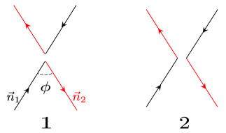
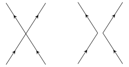
Figure 1: (a)𝑎(a) The figure eight Wilson loop with areas A¯1subscript¯𝐴1\bar{A}_{1} and A¯2subscript¯𝐴2\bar{A}_{2}. (b)𝑏(b) Two intersecting lines (left) and two touching lines (right) which mix under the renormalization group flow.

As an important application, we compute a small angle limit of the cross anomalous dimension of intersecting Wilson lines. The cross anomalous dimension controls the mixing of two different configurations of Wilson lines, two intersecting lines and two touching lines (see figure 1), under the renormalization group. It also describes the soft anomalous dimension, which controls how the soft gluons transfer the color degrees of freedom of partons in a scattering process. We generalize the analysis of the Bremsstrahlung function in [25, 26] and relate the small angle limit—and more generally the near-BPS limits—of these anomalous dimensions to our localization computations. The results are exact at finite λ𝜆\lambda and N𝑁N and reproduce the answers at weak coupling in the literature [27, 28, 29].

The formalism in this paper will be used in our upcoming paper [30] on the defect CFT correlators on the higher-rank Wilson loops. There, we consider a configuration in which multiple fundamental Wilson loops with different areas are joined together by a projector to a higher-rank representation. We compute its expectation value by taking an appropriate linear combination of multiply intersecting loops.

The rest of the paper is organized as follows. In section 2, we review the 1/8181/8 BPS Wilson loops and their relation to 2d YM. We then present a new integral representation for correlators of non-intersecting Wilson loops which simplifies the analysis of the loop equation in the subsequent sections. In section 3, we review the loop equation in 2d YM and solve it in the zero-instanton sector on S2superscript𝑆2S^{2}. As a result, we obtain a closed-form integral representation for intersecting loops. We then demonstrate how to evaluate the integral at large N𝑁N using examples of a figure eight loop and a two-intersection loop and study the weak- and strong-coupling limits. In section 4, we use these results to compute the small-angle and near-BPS limits of the cross anomalous dimension at finite λ𝜆\lambda and N𝑁N. We then discuss future directions in section 5. A few appendices are provided to explain technical details.

2 1/8 BPS Wilson Loop, 2d YM and Matrix Model

2.1 1/8 BPS Wilson loops and matrix model

In supersymmetric gauge theories, one can often define a supersymmetric generalization of the Wilson loop by coupling the loop to scalar fields. The 1/8181/8 BPS Wilson loop in 𝒩=4𝒩4\mathcal{N}=4 SYM is a special kind of such operators which can be defined for an arbitrary contour C𝐶C on S2superscript𝑆2S^{2} inside R4superscript𝑅4R^{4} or S4superscript𝑆4S^{4} (see figure 2):

𝒲1/8:=1NtrPexp(C(iAj+ϵkjlxkΦl)𝑑xj).assignsubscript𝒲181𝑁trPexpsubscriptcontour-integral𝐶𝑖subscript𝐴𝑗subscriptitalic-ϵ𝑘𝑗𝑙superscript𝑥𝑘superscriptΦ𝑙differential-dsuperscript𝑥𝑗\mathcal{W}_{1/8}:=\frac{1}{N}{\rm tr}\,{\rm Pexp}\left(\oint_{C}\left(iA_{j}+\epsilon_{kjl}x^{k}\Phi^{l}\right)dx^{j}\right)\,. (2.1)

Here all the indices run from 111 to 333 and xjsuperscript𝑥𝑗x^{j}’s are the coordinates of S2superscript𝑆2S^{2}, j=13(xj)2=1superscriptsubscript𝑗13superscriptsuperscript𝑥𝑗21\sum_{j=1}^{3}(x^{j})^{2}=1. Throughout this paper, we consider the U(N)𝑁(N) gauge group unless otherwise stated.

It was conjectured through the perturbative computations [12, 13] and later supported by the localization [11] that the computation of the 1/8181/8 BPS Wilson loop reduces to that of the standard Wilson loop in 2d YM on S2superscript𝑆2S^{2} in the zero-instanton sector,

𝒲1/8subscript𝒲18\displaystyle\mathcal{W}_{1/8} 𝒲2dYM:=1NtrPexp(CiAj𝑑xj),assignsubscript𝒲2dYM1𝑁trPexpsubscriptcontour-integral𝐶𝑖subscript𝐴𝑗differential-dsuperscript𝑥𝑗\displaystyle\longleftrightarrow\quad\mathcal{W}_{\text{2dYM}}:=\frac{1}{N}{\rm tr}\,{\rm Pexp}\left(\oint_{C}\,iA_{j}dx^{j}\right)\,, (2.2)

where the coupling constants of 2d YM (g2dsubscript𝑔2dg_{\rm 2d}) and 𝒩=4𝒩4\mathcal{N}=4 SYM (gYMsubscript𝑔YMg_{\rm YM}) are related by

g2d2=gYM22π,superscriptsubscript𝑔2d2superscriptsubscript𝑔YM22𝜋g_{\rm 2d}^{2}=-\frac{g_{\rm YM}^{2}}{2\pi}\,, (2.3)

and the action of 2d YM is

S2d=1g2d2d2σgtr(FμνFμν).subscript𝑆2𝑑1superscriptsubscript𝑔2d2superscript𝑑2𝜎𝑔trsubscript𝐹𝜇𝜈superscript𝐹𝜇𝜈S_{2d}=\frac{1}{g_{\rm 2d}^{2}}\int d^{2}\sigma\sqrt{g}{\rm tr}\left(F_{\mu\nu}F^{\mu\nu}\right)\,. (2.4)
Refer to caption
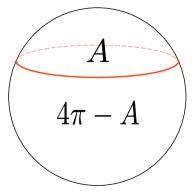
Figure 2: The 1/8181/8-BPS Wilson loop on S2superscript𝑆2S^{2}. The 1/8181/8-BPS loop can be defined on an arbitrary contour on S2superscript𝑆2S^{2} and its coupling to scalars is given by (2.1). A single loop divides S2superscript𝑆2S^{2} into two regions, one with area A𝐴A and the other with area 4πA4𝜋𝐴4\pi-A. Its expectation value depends only on the area A𝐴A owing to the relation to 2d YM.

The expectation value of a single 1/8181/8-BPS loop was computed by resumming the perturbative series in 2d YM and re-expressing it as a matrix integral111Z𝑍Z is a partition function of the matrix model, namely a matrix integral without the insertion of tr(eΦ)/Ntrsuperscript𝑒Φ𝑁{\rm tr}\left(e^{\Phi}\right)/N.,

𝒲1/8=1Z[dΦ]1Ntr(eΦ)e(4π)22A(4πA)gYM2tr(Φ2).delimited-⟨⟩subscript𝒲181𝑍delimited-[]𝑑Φ1𝑁trsuperscript𝑒Φsuperscript𝑒superscript4𝜋22𝐴4𝜋𝐴superscriptsubscript𝑔YM2trsuperscriptΦ2\displaystyle\langle\mathcal{W}_{1/8}\rangle=\frac{1}{Z}\int[d\Phi]\frac{1}{N}{\rm tr}\left(e^{\Phi}\right)e^{-\frac{(4\pi)^{2}}{2A(4\pi-A)g_{\rm YM}^{2}}{\rm tr}\left(\Phi^{2}\right)}\,. (2.5)

By evaluating this matrix integral, we get

𝒲1/8=1NLN11(λ4N)eλ8N,λ:=λ(1(A2π)24π2),formulae-sequencedelimited-⟨⟩subscript𝒲181𝑁superscriptsubscript𝐿𝑁11superscript𝜆4𝑁superscript𝑒superscript𝜆8𝑁assignsuperscript𝜆𝜆1superscript𝐴2𝜋24superscript𝜋2\langle\mathcal{W}_{1/8}\rangle=\frac{1}{N}L_{N-1}^{1}\left(-\frac{\lambda^{\prime}}{4N}\right)e^{\frac{\lambda^{\prime}}{8N}}\,,\qquad\lambda^{\prime}:=\lambda\left(1-\frac{(A-2\pi)^{2}}{4\pi^{2}}\right)\,, (2.6)

where λ:=gYM2Nassign𝜆superscriptsubscript𝑔YM2𝑁\lambda:=g_{\rm YM}^{2}N is the ’t Hooft coupling constant, LN11superscriptsubscript𝐿𝑁11L_{N-1}^{1} is an associated Laguerre polynomial and A𝐴A is the area of the region encircled by the Wilson loop. The large N𝑁N limit of this result gives a generalization of the famous result for the 1/2121/2-BPS Wilson loop,

𝒲1/8=N2λI1(λ),delimited-⟨⟩subscript𝒲18𝑁2superscript𝜆subscript𝐼1superscript𝜆\langle\mathcal{W}_{1/8}\rangle\overset{N\to\infty}{=}\frac{2}{\sqrt{\lambda^{\prime}}}I_{1}(\sqrt{\lambda^{\prime}})\,, (2.7)

with Insubscript𝐼𝑛I_{n} being the modified Bessel function.

As another application of the relation (2.2), a multi-matrix model for the correlation functions of 1/8181/8-BPS Wilson loops was derived in [17]. A heuristic way222See [17] for more rigorous discussions. to derive the matrix model is as follows: First we rewrite the action of 2d YM as a deformed BF theory,

S=tr(BF)g2d24d2σgtr(B2).𝑆tr𝐵𝐹superscriptsubscript𝑔2d24superscript𝑑2𝜎𝑔trsuperscript𝐵2S=\int{\rm tr}\left(B\wedge F\right)-\frac{g_{\rm 2d}^{2}}{4}\int d^{2}\sigma\sqrt{g}\,{\rm tr}\left(B^{2}\right)\,. (2.8)

If one integrates out B𝐵B, one recovers the standard 2d YM action. Second we use the fact that the theory reduces essentially to the abelian theory and localizes to configurations for which B𝐵B is piecewise constant with discontinuities across the Wilson loops. In such configurations, the first term of the action (2.8) becomes a boundary term

Σtr(BF)=tr[BΣA]=itr[BX],subscriptΣtr𝐵𝐹trdelimited-[]𝐵subscriptΣ𝐴𝑖trdelimited-[]𝐵𝑋\int_{\Sigma}{\rm tr}(B\wedge F)={\rm tr}\left[B\int_{\partial\Sigma}A\right]=-i{\rm tr}\left[BX\right]\,, (2.9)

where ΣΣ\Sigma is a subregion of S2superscript𝑆2S^{2} whose boundaries are given by the Wilson loops and X:=iΣAassign𝑋𝑖subscriptΣ𝐴X:=i\int_{\partial\Sigma}A is a boundary holonomy. On the other hand the second term simply gives

g2d24Σd2σgtr(B2)=g2d2AΣ4tr(B2)=gYM2AΣ8πtr(B2),superscriptsubscript𝑔2d24subscriptΣsuperscript𝑑2𝜎𝑔trsuperscript𝐵2superscriptsubscript𝑔2d2subscript𝐴Σ4trsuperscript𝐵2superscriptsubscript𝑔YM2subscript𝐴Σ8𝜋trsuperscript𝐵2-\frac{g_{\rm 2d}^{2}}{4}\int_{\Sigma}d^{2}\sigma\sqrt{g}\,{\rm tr}\left(B^{2}\right)=-\frac{g_{\rm 2d}^{2}A_{\Sigma}}{4}{\rm tr}(B^{2})=\frac{g_{\rm YM}^{2}A_{\Sigma}}{8\pi}{\rm tr}(B^{2})\,, (2.10)

where AΣsubscript𝐴ΣA_{\Sigma} is the area of the region ΣΣ\Sigma.

Performing such rewritings to each region ΣmsubscriptΣ𝑚\Sigma_{m}, we obtain the following multi-matrix model action:

S^^𝑆\displaystyle\hat{S} ={Σm}[itr(jΣmsj(m)B^ΣmX^j)+gYM2AΣm8πtr(B^Σm2)].absentsubscriptsubscriptΣ𝑚delimited-[]𝑖trsubscript𝑗subscriptΣ𝑚superscriptsubscript𝑠𝑗𝑚subscript^𝐵subscriptΣ𝑚subscript^𝑋𝑗superscriptsubscript𝑔YM2subscript𝐴subscriptΣ𝑚8𝜋trsuperscriptsubscript^𝐵subscriptΣ𝑚2\displaystyle=\sum_{\{\Sigma_{m}\}}\left[-i{\rm tr}\left(\sum_{j\in\partial\Sigma_{m}}s_{j}^{(m)}\hat{B}_{\Sigma_{m}}\hat{X}_{j}\right)+\frac{g_{\rm YM}^{2}A_{\Sigma_{m}}}{8\pi}{\rm tr}\left(\hat{B}_{\Sigma_{m}}^{2}\right)\right]\,. (2.11)

Here sj(m)superscriptsubscript𝑠𝑗𝑚s_{j}^{(m)} is an orientation factor which takes value +11+1 when the holonomy X^jsubscript^𝑋𝑗\hat{X}_{j} is oriented in the same direction as the boundary ΣmsubscriptΣ𝑚\partial\Sigma_{m}, and 11-1 otherwise. From this action, the correlator of the Wilson loops can be computed as follows,

k𝒲k=[dB^Σm][dX^j]ktrrk(eX^k)eS^[dB^Σm][dX^j]eS^,delimited-⟨⟩subscriptproduct𝑘subscript𝒲𝑘delimited-[]𝑑subscript^𝐵subscriptΣ𝑚delimited-[]𝑑subscript^𝑋𝑗subscriptproduct𝑘subscripttrsubscript𝑟𝑘superscript𝑒subscript^𝑋𝑘superscript𝑒^𝑆delimited-[]𝑑subscript^𝐵subscriptΣ𝑚delimited-[]𝑑subscript^𝑋𝑗superscript𝑒^𝑆\displaystyle\left<\prod_{k}\mathcal{W}_{k}\right>=\frac{\int[d\hat{B}_{\Sigma_{m}}][d\hat{X}_{j}]\prod_{k}{\rm tr}_{r_{k}}(e^{\hat{X}_{k}})e^{-\hat{S}}}{\int[d\hat{B}_{\Sigma_{m}}][d\hat{X}_{j}]e^{-\hat{S}}}\,, (2.12)

where rksubscript𝑟𝑘r_{k} is the representation of the k𝑘k-th Wilson loop 𝒲ksubscript𝒲𝑘\mathcal{W}_{k}. As was done in [17], one can integrate out B^Σmsubscript^𝐵subscriptΣ𝑚\hat{B}_{\Sigma_{m}}’s and obtain an action purely in terms of X^jsubscript^𝑋𝑗\hat{X}_{j}’s. This however is not convenient for analyzing the loop equation since the resulting action depends nonlinearly on the areas AΣmsubscript𝐴subscriptΣ𝑚A_{\Sigma_{m}}. In this paper, we instead integrate out X^jsubscript^𝑋𝑗\hat{X}_{j} and derive a new integral representation which is more convenient for the application of the loop equation.

2.2 A new integral representation for Wilson loop correlators

To derive an integral representation, it is convenient to first rescale the matrices as

Xj:=4πX^jgYM2,BΣm:=gYM2B^Σm4π.formulae-sequenceassignsubscript𝑋𝑗4𝜋subscript^𝑋𝑗superscriptsubscript𝑔YM2assignsubscript𝐵subscriptΣ𝑚superscriptsubscript𝑔YM2subscript^𝐵subscriptΣ𝑚4𝜋X_{j}:=\frac{4\pi\hat{X}_{j}}{g_{\rm YM}^{2}}\,,\qquad\qquad B_{\Sigma_{m}}:=\frac{g_{\rm YM}^{2}\hat{B}_{\Sigma_{m}}}{4\pi}\,. (2.13)

Then, the action and the correlator read

S={Σm}[itr(jΣmsj(m)BΣmXj)+2πAΣmgYM2tr(BΣm2)],𝑆subscriptsubscriptΣ𝑚delimited-[]𝑖trsubscript𝑗subscriptΣ𝑚superscriptsubscript𝑠𝑗𝑚subscript𝐵subscriptΣ𝑚subscript𝑋𝑗2𝜋subscript𝐴subscriptΣ𝑚superscriptsubscript𝑔YM2trsuperscriptsubscript𝐵subscriptΣ𝑚2\displaystyle S=\sum_{\{\Sigma_{m}\}}\left[-i{\rm tr}\left(\sum_{j\in\partial\Sigma_{m}}s_{j}^{(m)}B_{\Sigma_{m}}X_{j}\right)+\frac{2\pi A_{\Sigma_{m}}}{g_{\rm YM}^{2}}{\rm tr}\left(B_{\Sigma_{m}}^{2}\right)\right]\,, (2.14)
k𝒲k=[dBΣm][dXj]ktrrk(eϵXk)eS[dBΣm][dXj]eS,delimited-⟨⟩subscriptproduct𝑘subscript𝒲𝑘delimited-[]𝑑subscript𝐵subscriptΣ𝑚delimited-[]𝑑subscript𝑋𝑗subscriptproduct𝑘subscripttrsubscript𝑟𝑘superscript𝑒italic-ϵsubscript𝑋𝑘superscript𝑒𝑆delimited-[]𝑑subscript𝐵subscriptΣ𝑚delimited-[]𝑑subscript𝑋𝑗superscript𝑒𝑆\displaystyle\left<\prod_{k}\mathcal{W}_{k}\right>=\frac{\int[dB_{\Sigma_{m}}][dX_{j}]\prod_{k}{\rm tr}_{r_{k}}(e^{\epsilon X_{k}})e^{-S}}{\int[dB_{\Sigma_{m}}][dX_{j}]e^{-S}}\,,

with

ϵ:=gYM24π=λ4πN=4πg2N.assignitalic-ϵsuperscriptsubscript𝑔YM24𝜋𝜆4𝜋𝑁4𝜋superscript𝑔2𝑁\epsilon:=\frac{g_{\rm YM}^{2}}{4\pi}=\frac{\lambda}{4\pi N}=\frac{4\pi g^{2}}{N}\,. (2.15)

In the last equality, we used the notation for the ’t Hooft coupling constant commonly used in the integrability literature,

g2:=λ16π2.assignsuperscript𝑔2𝜆16superscript𝜋2g^{2}:=\frac{\lambda}{16\pi^{2}}\,. (2.16)

2.2.1 A single fundamental loop

Let us first discuss the expectation value of a single fundamental Wilson loop with no self-intersections. In the presence of a Wilson loop, S2superscript𝑆2S^{2} is divided into two regions, one with the area 4πA(=:A0)4\pi-A(=:A_{0}) and the other with the area A(=:A1)A(=:A_{1}) (see figure 2), and the action of the matrix model reads

S=2πA0gYM2tr(B02)+2πA1gYM2tr(B12)itr(X(B0B1)).𝑆2𝜋subscript𝐴0superscriptsubscript𝑔YM2trsuperscriptsubscript𝐵022𝜋subscript𝐴1superscriptsubscript𝑔YM2trsuperscriptsubscript𝐵12𝑖tr𝑋subscript𝐵0subscript𝐵1S=\frac{2\pi A_{0}}{g_{\rm YM}^{2}}{\rm tr}(B_{0}^{2})+\frac{2\pi A_{1}}{g_{\rm YM}^{2}}{\rm tr}(B_{1}^{2})-i{\rm tr}\left(X(B_{0}-B_{1})\right)\,. (2.17)

To compute the expectation value of the Wilson loop in this matrix model, we use the Harish-Chandra-Itzykson-Zuber identity

𝑑Ωeitr(ΩAΩB)=deteiaibjΔ(a)Δ(b),differential-dΩsuperscript𝑒𝑖trsuperscriptΩ𝐴Ω𝐵superscript𝑒𝑖subscript𝑎𝑖subscript𝑏𝑗Δ𝑎Δ𝑏\int d\Omega\,e^{i{\rm tr}\left(\Omega^{\dagger}A\Omega B\right)}=\frac{\det e^{ia_{i}b_{j}}}{\Delta(a)\Delta(b)}\,, (2.18)

where A𝐴A and B𝐵B are diagonal matrices with entries ajsubscript𝑎𝑗a_{j}’s and bjsubscript𝑏𝑗b_{j}’s respectively, 𝑑Ωdifferential-dΩ\int d\Omega is an integral over the unitary matrices and ΔΔ\Delta is the Vandermonde determinant Δ(a):=i<j(aiaj)assignΔ𝑎subscriptproduct𝑖𝑗subscript𝑎𝑖subscript𝑎𝑗\Delta(a):=\prod_{i<j}(a_{i}-a_{j}).

Using (2.18), we can reduce the partition function of the matrix model (2.17) to integrals of eigenvalues,

Z=[dX][dB0][dB1]eS=dNxdNb(0)dNb(1),𝑍delimited-[]𝑑𝑋delimited-[]𝑑subscript𝐵0delimited-[]𝑑subscript𝐵1superscript𝑒𝑆superscript𝑑𝑁𝑥superscript𝑑𝑁superscript𝑏0superscript𝑑𝑁superscript𝑏1Z=\int[dX][dB_{0}][dB_{1}]\,\,e^{-S}=\int d^{N}x\,d^{N}b^{(0)}\,d^{N}b^{(1)}\,\,\mathcal{I}\,, (2.19)

where the integrand \mathcal{I} is given by

\displaystyle\mathcal{I} =Δ2(x)Δ2(b(0))Δ2(b(1))deteixibj(0)deteixkbl(1)Δ2(x)Δ(b(0))Δ(b(1))e2πgYM2j(A0(bj(0))2+A1(bj(1))2)absentsuperscriptΔ2𝑥superscriptΔ2superscript𝑏0superscriptΔ2superscript𝑏1superscript𝑒𝑖subscript𝑥𝑖subscriptsuperscript𝑏0𝑗superscript𝑒𝑖subscript𝑥𝑘subscriptsuperscript𝑏1𝑙superscriptΔ2𝑥Δsuperscript𝑏0Δsuperscript𝑏1superscript𝑒2𝜋superscriptsubscript𝑔YM2subscript𝑗subscript𝐴0superscriptsuperscriptsubscript𝑏𝑗02subscript𝐴1superscriptsuperscriptsubscript𝑏𝑗12\displaystyle=\Delta^{2}(x)\Delta^{2}(b^{(0)})\Delta^{2}(b^{(1)})\frac{\det e^{ix_{i}b^{(0)}_{j}}\det e^{-ix_{k}b^{(1)}_{l}}}{\Delta^{2}(x)\Delta(b^{(0)})\Delta(b^{(1)})}\,\,e^{-\frac{2\pi}{g_{\rm YM}^{2}}\sum_{j}(A_{0}(b_{j}^{(0)})^{2}+A_{1}(b_{j}^{(1)})^{2})} (2.20)
=Δ(b(0))Δ(b(1))deteixibj(0)deteixkbl(1)e2πgYM2j(A0(bj(0))2+A1(bj(1))2).absentΔsuperscript𝑏0Δsuperscript𝑏1superscript𝑒𝑖subscript𝑥𝑖subscriptsuperscript𝑏0𝑗superscript𝑒𝑖subscript𝑥𝑘subscriptsuperscript𝑏1𝑙superscript𝑒2𝜋superscriptsubscript𝑔YM2subscript𝑗subscript𝐴0superscriptsuperscriptsubscript𝑏𝑗02subscript𝐴1superscriptsuperscriptsubscript𝑏𝑗12\displaystyle=\Delta(b^{(0)})\Delta(b^{(1)})\det e^{ix_{i}b^{(0)}_{j}}\det e^{-ix_{k}b^{(1)}_{l}}\,\,e^{-\frac{2\pi}{g_{\rm YM}^{2}}\sum_{j}(A_{0}(b_{j}^{(0)})^{2}+A_{1}(b_{j}^{(1)})^{2})}\,.

We next expand the determinants into a sum over permutations:

deteixibj(0)=σSN(1)σjeixibσj(0),deteixkbl(1)=σSN(1)σjeixibσj(1).formulae-sequencesuperscript𝑒𝑖subscript𝑥𝑖subscriptsuperscript𝑏0𝑗subscript𝜎subscript𝑆𝑁superscript1𝜎subscriptproduct𝑗superscript𝑒𝑖subscript𝑥𝑖subscriptsuperscript𝑏0subscript𝜎𝑗superscript𝑒𝑖subscript𝑥𝑘subscriptsuperscript𝑏1𝑙subscriptsuperscript𝜎subscript𝑆𝑁superscript1superscript𝜎subscriptproduct𝑗superscript𝑒𝑖subscript𝑥𝑖subscriptsuperscript𝑏1subscript𝜎𝑗\det e^{ix_{i}b^{(0)}_{j}}=\sum_{\sigma\in S_{N}}(-1)^{\sigma}\prod_{j}e^{ix_{i}b^{(0)}_{\sigma_{j}}}\,,\qquad\det e^{-ix_{k}b^{(1)}_{l}}=\sum_{\sigma^{\prime}\in S_{N}}(-1)^{\sigma^{\prime}}\prod_{j}e^{-ix_{i}b^{(1)}_{\sigma_{j}}}\,. (2.21)

Owing to the symmetry of the rest of the integrand, all these permutations give the same answer . We thus pick the simplest one (σj=jsubscript𝜎𝑗𝑗\sigma_{j}=j and σj=jsubscriptsuperscript𝜎𝑗𝑗\sigma^{\prime}_{j}=j) and multiply a factor (N!)2superscript𝑁2(N!)^{2}. After integrating out x𝑥x’s, we get

Z𝑍\displaystyle Z =(2π)N(N!)2(s=01dNb(s)Δ(b(s)))(kδ(bk(0)bk(1)))e2πgYM2j(A0(bj(0))2+A1(bj(1))2)absentsuperscript2𝜋𝑁superscript𝑁2superscriptsubscriptproduct𝑠01superscript𝑑𝑁superscript𝑏𝑠Δsuperscript𝑏𝑠subscriptproduct𝑘𝛿subscriptsuperscript𝑏0𝑘subscriptsuperscript𝑏1𝑘superscript𝑒2𝜋superscriptsubscript𝑔YM2subscript𝑗subscript𝐴0superscriptsuperscriptsubscript𝑏𝑗02subscript𝐴1superscriptsuperscriptsubscript𝑏𝑗12\displaystyle=(2\pi)^{N}(N!)^{2}\int\left(\prod_{s=0}^{1}d^{N}b^{(s)}\Delta(b^{(s)})\right)\left(\prod_{k}\delta(b^{(0)}_{k}-b^{(1)}_{k})\right)e^{-\frac{2\pi}{g_{\rm YM}^{2}}\sum_{j}(A_{0}(b_{j}^{(0)})^{2}+A_{1}(b_{j}^{(1)})^{2})} (2.22)
=(2π)N(N!)2dNbΔ2(b)e8π2gYM2j(bj)2.absentsuperscript2𝜋𝑁superscript𝑁2superscript𝑑𝑁𝑏superscriptΔ2𝑏superscript𝑒8superscript𝜋2superscriptsubscript𝑔YM2subscript𝑗superscriptsubscript𝑏𝑗2\displaystyle=(2\pi)^{N}(N!)^{2}\int d^{N}b\,\Delta^{2}(b)\,e^{-\frac{8\pi^{2}}{g_{\rm YM}^{2}}\sum_{j}(b_{j})^{2}}\,.

In the second line, we integrated out b(1)superscript𝑏1b^{(1)}’s and denoted the remaining variables bj(0)superscriptsubscript𝑏𝑗0b_{j}^{(0)} as bjsubscript𝑏𝑗b_{j}. We also used A0+A1=4πsubscript𝐴0subscript𝐴14𝜋A_{0}+A_{1}=4\pi to simplify the exponent.

Similarly, the expectation value of the fundamental Wilson loop can be reduced to the following eigenvalue integral:

𝒲delimited-⟨⟩𝒲\displaystyle\langle\mathcal{W}\rangle =1Z[dX][dB0][dB1]tr(eϵX)NeS=1ZdNxdNb(0)dNb(1)keϵxkN,absent1𝑍delimited-[]𝑑𝑋delimited-[]𝑑subscript𝐵0delimited-[]𝑑subscript𝐵1trsuperscript𝑒italic-ϵ𝑋𝑁superscript𝑒𝑆1𝑍superscript𝑑𝑁𝑥superscript𝑑𝑁superscript𝑏0superscript𝑑𝑁superscript𝑏1subscript𝑘superscript𝑒italic-ϵsubscript𝑥𝑘𝑁\displaystyle=\frac{1}{Z}\int[dX][dB_{0}][dB_{1}]\frac{{\rm tr}\left(e^{\epsilon X}\right)}{N}e^{-S}=\frac{1}{Z}\int d^{N}x\,d^{N}b^{(0)}\,d^{N}b^{(1)}\,\,\mathcal{I}\,\,\frac{\sum_{k}e^{\epsilon x_{k}}}{N}\,, (2.23)

with \mathcal{I} defined in (2.20). To evaluate this integral, we again expand the determinants and integrate out x𝑥x’s. The only modification is that one of the delta functions gets shifted by iϵ𝑖italic-ϵ-i\epsilon owing to the factor eϵxksuperscript𝑒italic-ϵsubscript𝑥𝑘e^{\epsilon x_{k}}. We then get

𝒲=delimited-⟨⟩𝒲absent\displaystyle\langle\mathcal{W}\rangle= (2π)N(N!)2Z(s=01dNb(s)Δ(b(s)))kδ(bk(0)bk(1)iϵ)Nsuperscript2𝜋𝑁superscript𝑁2𝑍superscriptsubscriptproduct𝑠01superscript𝑑𝑁superscript𝑏𝑠Δsuperscript𝑏𝑠subscript𝑘𝛿superscriptsubscript𝑏𝑘0superscriptsubscript𝑏𝑘1𝑖italic-ϵ𝑁\displaystyle\frac{(2\pi)^{N}(N!)^{2}}{Z}\int\left(\prod_{s=0}^{1}d^{N}b^{(s)}\Delta(b^{(s)})\right)\sum_{k}\frac{\delta(b_{k}^{(0)}-b_{k}^{(1)}-i\epsilon)}{N} (2.24)
×(jkδ(bj(0)bj(1)))e2πgYM2j(A0(bj(0))2+A1(bj(1))2)absentsubscriptproduct𝑗𝑘𝛿subscriptsuperscript𝑏0𝑗subscriptsuperscript𝑏1𝑗superscript𝑒2𝜋superscriptsubscript𝑔YM2subscript𝑗subscript𝐴0superscriptsuperscriptsubscript𝑏𝑗02subscript𝐴1superscriptsuperscriptsubscript𝑏𝑗12\displaystyle\times\left(\prod_{j\neq k}\delta(b^{(0)}_{j}-b^{(1)}_{j})\right)e^{-\frac{2\pi}{g_{\rm YM}^{2}}\sum_{j}(A_{0}(b_{j}^{(0)})^{2}+A_{1}(b_{j}^{(1)})^{2})}
=\displaystyle= (2π)N(N!)2ZdNbΔ2(b)e8π2gYM2j(bj)2keiA1(bkiϵ2)jkbkbjiϵbkbjN.superscript2𝜋𝑁superscript𝑁2𝑍superscript𝑑𝑁𝑏superscriptΔ2𝑏superscript𝑒8superscript𝜋2superscriptsubscript𝑔YM2subscript𝑗superscriptsubscript𝑏𝑗2subscript𝑘superscript𝑒𝑖subscript𝐴1subscript𝑏𝑘𝑖italic-ϵ2subscriptproduct𝑗𝑘subscript𝑏𝑘subscript𝑏𝑗𝑖italic-ϵsubscript𝑏𝑘subscript𝑏𝑗𝑁\displaystyle\frac{(2\pi)^{N}(N!)^{2}}{Z}\int d^{N}b\,\,\Delta^{2}(b)e^{-\frac{8\pi^{2}}{g_{\rm YM}^{2}}\sum_{j}(b_{j})^{2}}\frac{\sum_{k}e^{iA_{1}(b_{k}-\frac{i\epsilon}{2})}\prod_{j\neq k}\frac{b_{k}-b_{j}-i\epsilon}{b_{k}-b_{j}}}{N}\,.

Now the crucial observation is that the sum ksubscript𝑘\sum_{k} can be recast into a contour integral,

𝒲delimited-⟨⟩𝒲\displaystyle\langle\mathcal{W}\rangle =(2π)N(N!)2ZdNbΔ2(b)e8π2gYM2j(bj)2[𝒞du8π2g2eiA1(uiϵ2)jubjiϵubj].absentsuperscript2𝜋𝑁superscript𝑁2𝑍superscript𝑑𝑁𝑏superscriptΔ2𝑏superscript𝑒8superscript𝜋2superscriptsubscript𝑔YM2subscript𝑗superscriptsubscript𝑏𝑗2delimited-[]subscriptcontour-integral𝒞𝑑𝑢8superscript𝜋2superscript𝑔2superscript𝑒𝑖subscript𝐴1𝑢𝑖italic-ϵ2subscriptproduct𝑗𝑢subscript𝑏𝑗𝑖italic-ϵ𝑢subscript𝑏𝑗\displaystyle=\frac{(2\pi)^{N}(N!)^{2}}{Z}\int d^{N}b\,\,\Delta^{2}(b)e^{-\frac{8\pi^{2}}{g_{\rm YM}^{2}}\sum_{j}(b_{j})^{2}}\left[\oint_{\mathcal{C}}\frac{du}{8\pi^{2}g^{2}}e^{iA_{1}(u-\frac{i\epsilon}{2})}\prod_{j}\frac{u-b_{j}-i\epsilon}{u-b_{j}}\right]\,. (2.25)

We can then interpret this as an expectation value of a Gaussian matrix model and get

𝒲=𝒞du8π2g2fA1(u)M.delimited-⟨⟩𝒲subscriptdelimited-⟨⟩subscriptcontour-integral𝒞𝑑𝑢8superscript𝜋2superscript𝑔2subscript𝑓subscript𝐴1𝑢𝑀\langle\mathcal{W}\rangle=\left<\oint_{\mathcal{C}}\frac{du}{8\pi^{2}g^{2}}f_{A_{1}}(u)\right>_{M}\,. (2.26)

Here the integration contour 𝒞𝒞\mathcal{C} encircles all the eigenvalues bksubscript𝑏𝑘b_{k}’s and fAsubscript𝑓𝐴f_{A} is given by

fA(u):=eiA(uiϵ2)det[uMiϵuM].assignsubscript𝑓𝐴𝑢superscript𝑒𝑖𝐴𝑢𝑖italic-ϵ2delimited-[]𝑢𝑀𝑖italic-ϵ𝑢𝑀f_{A}(u):=e^{iA(u-\frac{i\epsilon}{2})}\det\left[\frac{u-M-i\epsilon}{u-M}\right]\,. (2.27)

The symbol Msubscriptdelimited-⟨⟩𝑀\left<\bullet\right>_{M} denotes the expectation value of \bullet in a Gaussian matrix model with the action SM:=8π2tr(M2)/gYM2assignsubscript𝑆𝑀8superscript𝜋2trsuperscript𝑀2superscriptsubscript𝑔YM2S_{M}:=8\pi^{2}{\rm tr}\left(M^{2}\right)/g_{\rm YM}^{2}:

M:=[dM]eSM[dM]eSM.assignsubscriptdelimited-⟨⟩𝑀delimited-[]𝑑𝑀superscript𝑒subscript𝑆𝑀delimited-[]𝑑𝑀superscript𝑒subscript𝑆𝑀\left<\bullet\right>_{M}:=\frac{\int[dM]\,\bullet\,e^{-S_{M}}}{\int[dM]\,e^{-S_{M}}}\,. (2.28)

The result (2.26) may appear more complicated than the expressions known in the literature [12, 13]. However, for the analysis of the loop equation, (2.26) is more convenient since the area-dependence is simple. See section 3 for more details.

2.2.2 Multiple fundamental loops

We now generalize the result (2.26) to correlators of multiple Wilson loops.
Refer to caption
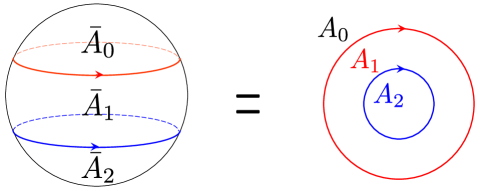
Figure 3: Two 1/8181/8-BPS loops with the same orientations. Left: The loops divide S2superscript𝑆2S^{2} into three disconnected regions with areas A¯0subscript¯𝐴0\bar{A}_{0}, A¯1subscript¯𝐴1\bar{A}_{1} and A¯2subscript¯𝐴2\bar{A}_{2}. Right: The same configuration viewed from the south pole. We denote the areas inside outer (red) and inner (blue) circles by A1subscript𝐴1A_{1} and A2subscript𝐴2A_{2} respectively and the area of the complement by A0subscript𝐴0A_{0}. The two sets of areas are related by A¯0=A0subscript¯𝐴0subscript𝐴0\bar{A}_{0}=A_{0}, A¯1=A1A2subscript¯𝐴1subscript𝐴1subscript𝐴2\bar{A}_{1}=A_{1}-A_{2} and A¯2=A2subscript¯𝐴2subscript𝐴2\bar{A}_{2}=A_{2}.

To see how it works, let us first consider the correlator of two fundamental Wilson loops with the same orientation. As depicted in figure 3, we denote the areas inside outer and inner loops by A1subscript𝐴1A_{1} and A2subscript𝐴2A_{2} respectively and the area of the complement by A0subscript𝐴0A_{0}. Then the matrix model action is given by

S=s=022πA¯sgYM2tr(Bs2)is=1,2tr(Xs(Bs1Bs)),𝑆superscriptsubscript𝑠022𝜋subscript¯𝐴𝑠superscriptsubscript𝑔YM2trsuperscriptsubscript𝐵𝑠2𝑖subscript𝑠12trsubscript𝑋𝑠subscript𝐵𝑠1subscript𝐵𝑠S=\sum_{s=0}^{2}\frac{2\pi\bar{A}_{s}}{g_{\rm YM}^{2}}{\rm tr}(B_{s}^{2})-i\sum_{s=1,2}{\rm tr}\left(X_{s}(B_{s-1}-B_{s})\right)\,, (2.29)

with A¯0:=A0assignsubscript¯𝐴0subscript𝐴0\bar{A}_{0}:=A_{0}, A¯1:=A1A2assignsubscript¯𝐴1subscript𝐴1subscript𝐴2\bar{A}_{1}:=A_{1}-A_{2} and A¯2:=A2assignsubscript¯𝐴2subscript𝐴2\bar{A}_{2}:=A_{2}. By reducing the matrix integral to the eigenvalues using the identity (2.18), we get

Z=(s=02[dBs])(s=1,2[dXs])eS=(s=02dNb(s))(s=1,2dNx(s))2,𝑍superscriptsubscriptproduct𝑠02delimited-[]𝑑subscript𝐵𝑠subscriptproduct𝑠12delimited-[]𝑑subscript𝑋𝑠superscript𝑒𝑆superscriptsubscriptproduct𝑠02superscript𝑑𝑁superscript𝑏𝑠subscriptproduct𝑠12superscript𝑑𝑁superscript𝑥𝑠subscript2Z=\int\left(\prod_{s=0}^{2}[dB_{s}]\right)\left(\prod_{s=1,2}[dX_{s}]\right)e^{-S}=\int\left(\prod_{s=0}^{2}d^{N}b^{(s)}\right)\left(\prod_{s=1,2}d^{N}x^{(s)}\right)\mathcal{I}_{2}\,, (2.30)

with

2=Δ(b(0))Δ(b(2))(s=12deteixi(s)bj(s1)deteixi(s)bj(s))e2πgYM2s=02jA¯s(bj(s))2subscript2Δsuperscript𝑏0Δsuperscript𝑏2superscriptsubscriptproduct𝑠12superscript𝑒𝑖superscriptsubscript𝑥𝑖𝑠superscriptsubscript𝑏𝑗𝑠1superscript𝑒𝑖superscriptsubscript𝑥𝑖𝑠superscriptsubscript𝑏𝑗𝑠superscript𝑒2𝜋superscriptsubscript𝑔YM2superscriptsubscript𝑠02subscript𝑗subscript¯𝐴𝑠superscriptsuperscriptsubscript𝑏𝑗𝑠2\displaystyle\mathcal{I}_{2}=\Delta(b^{(0)})\Delta(b^{(2)})\left(\prod_{s=1}^{2}\det e^{ix_{i}^{(s)}b_{j}^{(s-1)}}\det e^{-ix_{i}^{(s)}b_{j}^{(s)}}\right)e^{-\frac{2\pi}{g_{\rm YM}^{2}}\sum_{s=0}^{2}\sum_{j}\bar{A}_{s}(b_{j}^{(s)})^{2}} (2.31)

Expanding a product of determinants, we obtain a sum of permutations

s=12deteixi(s)bj(s1)deteixi(s)bj(s)=σ0,σ1,σ2,σ3(1)sσsjei(bσj0(0)bσj1(1))xj(1)ei(bσj2(1)bσj3(2))xj(2).superscriptsubscriptproduct𝑠12superscript𝑒𝑖superscriptsubscript𝑥𝑖𝑠superscriptsubscript𝑏𝑗𝑠1superscript𝑒𝑖superscriptsubscript𝑥𝑖𝑠superscriptsubscript𝑏𝑗𝑠subscriptsuperscript𝜎0superscript𝜎1superscript𝜎2superscript𝜎3superscript1subscript𝑠superscript𝜎𝑠subscriptproduct𝑗superscript𝑒𝑖subscriptsuperscript𝑏0subscriptsuperscript𝜎0𝑗subscriptsuperscript𝑏1subscriptsuperscript𝜎1𝑗superscriptsubscript𝑥𝑗1superscript𝑒𝑖subscriptsuperscript𝑏1subscriptsuperscript𝜎2𝑗subscriptsuperscript𝑏2subscriptsuperscript𝜎3𝑗superscriptsubscript𝑥𝑗2\displaystyle\prod_{s=1}^{2}\det e^{ix_{i}^{(s)}b_{j}^{(s-1)}}\det e^{-ix_{i}^{(s)}b_{j}^{(s)}}=\sum_{\sigma^{0},\sigma^{1},\sigma^{2},\sigma^{3}}(-1)^{\sum_{s}\sigma^{s}}\prod_{j}e^{i(b^{(0)}_{\sigma^{0}_{j}}-b^{(1)}_{\sigma^{1}_{j}})x_{j}^{(1)}}e^{i(b^{(1)}_{\sigma^{2}_{j}}-b^{(2)}_{\sigma^{3}_{j}})x_{j}^{(2)}}\,. (2.32)

Again all these permutations turn out to give the same result owing to the symmetry of the integrand. We can therefore replace the integrand 2subscript2\mathcal{I}_{2} with

2=(N!)4Δ(b(0))Δ(b(2))(jei(bj(0)bj(1))xj(1)ei(bj(1)bj(2))xj(2))e2πgYM2s=02jA¯s(bj(s))2.subscript2superscript𝑁4Δsuperscript𝑏0Δsuperscript𝑏2subscriptproduct𝑗superscript𝑒𝑖superscriptsubscript𝑏𝑗0superscriptsubscript𝑏𝑗1superscriptsubscript𝑥𝑗1superscript𝑒𝑖superscriptsubscript𝑏𝑗1superscriptsubscript𝑏𝑗2superscriptsubscript𝑥𝑗2superscript𝑒2𝜋superscriptsubscript𝑔YM2superscriptsubscript𝑠02subscript𝑗subscript¯𝐴𝑠superscriptsuperscriptsubscript𝑏𝑗𝑠2\displaystyle\mathcal{I}_{2}=(N!)^{4}\Delta(b^{(0)})\Delta(b^{(2)})\left(\prod_{j}e^{i(b_{j}^{(0)}-b_{j}^{(1)})x_{j}^{(1)}}e^{i(b_{j}^{(1)}-b_{j}^{(2)})x_{j}^{(2)}}\right)e^{-\frac{2\pi}{g_{\rm YM}^{2}}\sum_{s=0}^{2}\sum_{j}\bar{A}_{s}(b_{j}^{(s)})^{2}}\,. (2.33)

Plugging this expression into (2.30), we find that the integrals of xj(k)superscriptsubscript𝑥𝑗𝑘x_{j}^{(k)} give the delta functions δ(bj(0)bj(1))𝛿subscriptsuperscript𝑏0𝑗subscriptsuperscript𝑏1𝑗\delta(b^{(0)}_{j}-b^{(1)}_{j}) and δ(bj(1)bj(2))𝛿subscriptsuperscript𝑏1𝑗subscriptsuperscript𝑏2𝑗\delta(b^{(1)}_{j}-b^{(2)}_{j}). Performing the integrals of b(1)superscript𝑏1b^{(1)} and b(2)superscript𝑏2b^{(2)}, we get

Z=(2π)2N(N!)4dNbΔ2(b)e8π2gYM2j(bj)2.𝑍superscript2𝜋2𝑁superscript𝑁4superscript𝑑𝑁𝑏superscriptΔ2𝑏superscript𝑒8superscript𝜋2superscriptsubscript𝑔YM2subscript𝑗superscriptsubscript𝑏𝑗2Z=(2\pi)^{2N}(N!)^{4}\int d^{N}b\,\,\Delta^{2}(b)\,\,e^{-\frac{8\pi^{2}}{g_{\rm YM}^{2}}\sum_{j}(b_{j})^{2}}\,. (2.34)

Here we again denoted bj(0)subscriptsuperscript𝑏0𝑗b^{(0)}_{j} by bjsubscript𝑏𝑗b_{j} and used sAs=4πsubscript𝑠subscript𝐴𝑠4𝜋\sum_{s}A_{s}=4\pi.

To compute the correlator of the Wilson loops, we insert

1N2tr(eϵX1)tr(eϵX2)1N2n,meϵxn(1)+ϵxm(2),1superscript𝑁2trsuperscript𝑒italic-ϵsubscript𝑋1trsuperscript𝑒italic-ϵsubscript𝑋2maps-to1superscript𝑁2subscript𝑛𝑚superscript𝑒italic-ϵsuperscriptsubscript𝑥𝑛1italic-ϵsuperscriptsubscript𝑥𝑚2\frac{1}{N^{2}}{\rm tr}\left(e^{\epsilon X_{1}}\right){\rm tr}\left(e^{\epsilon X_{2}}\right)\quad\mapsto\quad\frac{1}{N^{2}}\sum_{n,m}e^{\epsilon x_{n}^{(1)}+\epsilon x_{m}^{(2)}}\,, (2.35)

to the partition function (2.30). We then obtain

𝒲1𝒲2=delimited-⟨⟩subscript𝒲1subscript𝒲2absent\displaystyle\langle\mathcal{W}_{1}\mathcal{W}_{2}\rangle= (2π)2N(N!)4Z(s=02dNb(s))Δ(b(0))Δ(b(2))e2πgYM2s=02jA¯s(bj(s))2superscript2𝜋2𝑁superscript𝑁4𝑍superscriptsubscriptproduct𝑠02superscript𝑑𝑁superscript𝑏𝑠Δsuperscript𝑏0Δsuperscript𝑏2superscript𝑒2𝜋superscriptsubscript𝑔YM2superscriptsubscript𝑠02subscript𝑗subscript¯𝐴𝑠superscriptsuperscriptsubscript𝑏𝑗𝑠2\displaystyle\frac{(2\pi)^{2N}(N!)^{4}}{Z}\int\left(\prod_{s=0}^{2}d^{N}b^{(s)}\right)\Delta(b^{(0)})\Delta(b^{(2)})e^{-\frac{2\pi}{g_{\rm YM}^{2}}\sum_{s=0}^{2}\sum_{j}\bar{A}_{s}(b_{j}^{(s)})^{2}} (2.36)
×n,mδ(bn(0)bn(1)iϵ)δ(bm(1)bm(2)iϵ)N2jnkmδ(bj(0)bj(1))δ(bk(1)bk(2)).\displaystyle\times\sum_{n,m}\frac{\delta(b_{n}^{(0)}-b_{n}^{(1)}-i\epsilon)\delta(b_{m}^{(1)}-b_{m}^{(2)}-i\epsilon)}{N^{2}}\prod_{\begin{subarray}{c}j\neq n\\ k\neq m\end{subarray}}\delta(b_{j}^{(0)}-b_{j}^{(1)})\delta(b_{k}^{(1)}-b_{k}^{(2)})\,.

To proceed, we split the sum into two parts,

n,m=nm+n=m,subscript𝑛𝑚subscript𝑛𝑚subscript𝑛𝑚\sum_{n,m}=\sum_{n\neq m}+\sum_{n=m}\,, (2.37)

integrate out bj(1,2)superscriptsubscript𝑏𝑗12b_{j}^{(1,2)}’s and recast the sums into integrals. The first term in (2.37) gives

𝒲1𝒲2nm=subscriptdelimited-⟨⟩subscript𝒲1subscript𝒲2𝑛𝑚absent\displaystyle\langle\mathcal{W}_{1}\mathcal{W}_{2}\rangle_{n\neq m}= (2π)2N(N!)4ZdNbΔ2(b)e8π2gYM2j(bj)2nmeiA1(bniϵ2)eiA2(bmiϵ2)N2superscript2𝜋2𝑁superscript𝑁4𝑍superscript𝑑𝑁𝑏superscriptΔ2𝑏superscript𝑒8superscript𝜋2superscriptsubscript𝑔YM2subscript𝑗superscriptsubscript𝑏𝑗2subscript𝑛𝑚superscript𝑒𝑖subscript𝐴1subscript𝑏𝑛𝑖italic-ϵ2superscript𝑒𝑖subscript𝐴2subscript𝑏𝑚𝑖italic-ϵ2superscript𝑁2\displaystyle\frac{(2\pi)^{2N}(N!)^{4}}{Z}\int d^{N}b\,\Delta^{2}(b)\,e^{-\frac{8\pi^{2}}{g_{\rm YM}^{2}}\sum_{j}(b_{j})^{2}}\sum_{n\neq m}\frac{e^{iA_{1}(b_{n}-\frac{i\epsilon}{2})}e^{iA_{2}(b_{m}-\frac{i\epsilon}{2})}}{N^{2}} (2.38)
×(bnbm)2(bnbm)2+ϵ2jnbnbjiϵbnbjkmbmbkiϵbmbk,absentsuperscriptsubscript𝑏𝑛subscript𝑏𝑚2superscriptsubscript𝑏𝑛subscript𝑏𝑚2superscriptitalic-ϵ2subscriptproduct𝑗𝑛subscript𝑏𝑛subscript𝑏𝑗𝑖italic-ϵsubscript𝑏𝑛subscript𝑏𝑗subscriptproduct𝑘𝑚subscript𝑏𝑚subscript𝑏𝑘𝑖italic-ϵsubscript𝑏𝑚subscript𝑏𝑘\displaystyle\times\frac{(b_{n}-b_{m})^{2}}{(b_{n}-b_{m})^{2}+\epsilon^{2}}\prod_{j\neq n}\frac{b_{n}-b_{j}-i\epsilon}{b_{n}-b_{j}}\prod_{k\neq m}\frac{b_{m}-b_{k}-i\epsilon}{b_{m}-b_{k}}\,,
=\displaystyle= (2π)2N(N!)4ZdNbΔ2(b)e8π2gYM2j(bj)2𝒞du1eiA1(u1iϵ2)8π2g2du2eiA2(u2iϵ2)8π2g2superscript2𝜋2𝑁superscript𝑁4𝑍superscript𝑑𝑁𝑏superscriptΔ2𝑏superscript𝑒8superscript𝜋2superscriptsubscript𝑔YM2subscript𝑗superscriptsubscript𝑏𝑗2subscriptcontour-integral𝒞𝑑subscript𝑢1superscript𝑒𝑖subscript𝐴1subscript𝑢1𝑖italic-ϵ28superscript𝜋2superscript𝑔2𝑑subscript𝑢2superscript𝑒𝑖subscript𝐴2subscript𝑢2𝑖italic-ϵ28superscript𝜋2superscript𝑔2\displaystyle\frac{(2\pi)^{2N}(N!)^{4}}{Z}\int d^{N}b\,\Delta^{2}(b)e^{-\frac{8\pi^{2}}{g_{\rm YM}^{2}}\sum_{j}(b_{j})^{2}}\oint_{\mathcal{C}}\frac{du_{1}\,e^{iA_{1}(u_{1}-\frac{i\epsilon}{2})}}{8\pi^{2}g^{2}}\frac{du_{2}\,e^{iA_{2}(u_{2}-\frac{i\epsilon}{2})}}{8\pi^{2}g^{2}}
×Δ¯(u1,u2)ju1bjiϵu1bjku2bkiϵu2bk,absent¯Δsubscript𝑢1subscript𝑢2subscriptproduct𝑗subscript𝑢1subscript𝑏𝑗𝑖italic-ϵsubscript𝑢1subscript𝑏𝑗subscriptproduct𝑘subscript𝑢2subscript𝑏𝑘𝑖italic-ϵsubscript𝑢2subscript𝑏𝑘\displaystyle\times\bar{\Delta}(u_{1},u_{2})\prod_{j}\frac{u_{1}-b_{j}-i\epsilon}{u_{1}-b_{j}}\prod_{k}\frac{u_{2}-b_{k}-i\epsilon}{u_{2}-b_{k}}\,,

where the “interaction term” Δ¯(u,v)¯Δ𝑢𝑣\bar{\Delta}(u,v) is given by

Δ¯(u,v):=(uv)2(uv)2+ϵ2.assign¯Δ𝑢𝑣superscript𝑢𝑣2superscript𝑢𝑣2superscriptitalic-ϵ2\bar{\Delta}(u,v):=\frac{(u-v)^{2}}{(u-v)^{2}+\epsilon^{2}}\,. (2.39)

Again (2.38) can be interpreted as an expectation value in the Gaussian matrix model

𝒲1𝒲2nm=𝒞du18π2g2du28π2g2Δ¯(u1,u2)fA1(u1)fA2(u2)M.subscriptdelimited-⟨⟩subscript𝒲1subscript𝒲2𝑛𝑚subscriptdelimited-⟨⟩subscriptcontour-integral𝒞𝑑subscript𝑢18superscript𝜋2superscript𝑔2𝑑subscript𝑢28superscript𝜋2superscript𝑔2¯Δsubscript𝑢1subscript𝑢2subscript𝑓subscript𝐴1subscript𝑢1subscript𝑓subscript𝐴2subscript𝑢2𝑀\langle\mathcal{W}_{1}\mathcal{W}_{2}\rangle_{n\neq m}=\left<\oint_{\mathcal{C}}\frac{du_{1}}{8\pi^{2}g^{2}}\frac{du_{2}}{8\pi^{2}g^{2}}\bar{\Delta}(u_{1},u_{2})f_{A_{1}}(u_{1})f_{A_{2}}(u_{2})\right>_{M}\,. (2.40)

Similarly, the second term in (2.37) gives333The term (2.41) resembles the “bound-state” contribution in the hexagon approach to the correlation functions [31, 32]. See also the comments below (2.47).

𝒲1𝒲2n=m=subscriptdelimited-⟨⟩subscript𝒲1subscript𝒲2𝑛𝑚absent\displaystyle\langle\mathcal{W}_{1}\mathcal{W}_{2}\rangle_{n=m}= (2π)2N(N!)4ZdNbΔ2(b)e8π2gYM2j(bj)2neiA1(bniϵ/2)eiA2(bn3iϵ/2)N2superscript2𝜋2𝑁superscript𝑁4𝑍superscript𝑑𝑁𝑏superscriptΔ2𝑏superscript𝑒8superscript𝜋2superscriptsubscript𝑔YM2subscript𝑗superscriptsubscript𝑏𝑗2subscript𝑛superscript𝑒𝑖subscript𝐴1subscript𝑏𝑛𝑖italic-ϵ2superscript𝑒𝑖subscript𝐴2subscript𝑏𝑛3𝑖italic-ϵ2superscript𝑁2\displaystyle\frac{(2\pi)^{2N}(N!)^{4}}{Z}\int d^{N}b\,\Delta^{2}(b)e^{-\frac{8\pi^{2}}{g_{\rm YM}^{2}}\sum_{j}(b_{j})^{2}}\sum_{n}\frac{e^{iA_{1}(b_{n}-i\epsilon/2)}e^{iA_{2}(b_{n}-3i\epsilon/2)}}{N^{2}} (2.41)
×jnbnbj2iϵbnbj\displaystyle\times\prod_{j\neq n}\frac{b_{n}-b_{j}-2i\epsilon}{b_{n}-b_{j}}
=\displaystyle= 12N𝒞du8π2g2fA1(u)fA2(uiϵ)M.12𝑁subscriptdelimited-⟨⟩subscriptcontour-integral𝒞𝑑𝑢8superscript𝜋2superscript𝑔2subscript𝑓subscript𝐴1𝑢subscript𝑓subscript𝐴2𝑢𝑖italic-ϵ𝑀\displaystyle\frac{1}{2N}\left<\oint_{\mathcal{C}}\frac{du}{8\pi^{2}g^{2}}f_{A_{1}}(u)f_{A_{2}}(u-i\epsilon)\right>_{M}\,.

Thus the sum of the two contributions (2.40) and (2.41) gives

𝒲1𝒲2=delimited-⟨⟩subscript𝒲1subscript𝒲2absent\displaystyle\langle\mathcal{W}_{1}\mathcal{W}_{2}\rangle= (2.42)
𝒞du18π2g2du28π2g2Δ¯(u1,u2)fA1(u1)fA2(u2)M+12N𝒞du8π2g2fA1(u)fA2(uiϵ)M.subscriptdelimited-⟨⟩subscriptcontour-integral𝒞𝑑subscript𝑢18superscript𝜋2superscript𝑔2𝑑subscript𝑢28superscript𝜋2superscript𝑔2¯Δsubscript𝑢1subscript𝑢2subscript𝑓subscript𝐴1subscript𝑢1subscript𝑓subscript𝐴2subscript𝑢2𝑀12𝑁subscriptdelimited-⟨⟩subscriptcontour-integral𝒞𝑑𝑢8superscript𝜋2superscript𝑔2subscript𝑓subscript𝐴1𝑢subscript𝑓subscript𝐴2𝑢𝑖italic-ϵ𝑀\displaystyle\left<\oint_{\mathcal{C}}\frac{du_{1}}{8\pi^{2}g^{2}}\frac{du_{2}}{8\pi^{2}g^{2}}\,\,\bar{\Delta}(u_{1},u_{2})\,\,f_{A_{1}}(u_{1})f_{A_{2}}(u_{2})\right>_{M}+\frac{1}{2N}\left<\oint_{\mathcal{C}}\frac{du}{8\pi^{2}g^{2}}f_{A_{1}}(u)f_{A_{2}}(u-i\epsilon)\right>_{M}\,.
Refer to caption
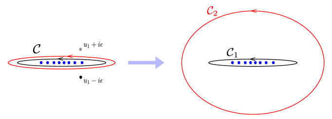
Figure 4: Deformation of the integration contours. Left: The integration contours for u1subscript𝑢1u_{1} (black) and u2subscript𝑢2u_{2} (red) in (2.42). The two contours are on top of each other and encircle the eigenvalues of M𝑀M (the blue dots in the figure). Right: The integration contours in (2.46). When we deform the contour of u2subscript𝑢2u_{2}, the integral picks up a contribution from poles at u2=u1±iϵsubscript𝑢2plus-or-minussubscript𝑢1𝑖italic-ϵu_{2}=u_{1}\pm i\epsilon (the gray and black dots). The residue at u1+iϵsubscript𝑢1𝑖italic-ϵu_{1}+i\epsilon turns out to vanish while the residue at u1iϵsubscript𝑢1𝑖italic-ϵu_{1}-i\epsilon cancels the second term in (2.42).

One can further simplify the expression by combining the two terms in (2.42): In the first term of (2.42), the integration contours of u1,2subscript𝑢12u_{1,2} are on top of each other and encircle all the eigenvalues of the matrix model (see figure 4). If one deforms the contour of u2subscript𝑢2u_{2} so that the two contours are far separated, the integral picks up a contribution from poles in the interaction term

Δ¯(u1,u2)=(u1u2)2(u1u2)2+ϵ2,¯Δsubscript𝑢1subscript𝑢2superscriptsubscript𝑢1subscript𝑢22superscriptsubscript𝑢1subscript𝑢22superscriptitalic-ϵ2\bar{\Delta}(u_{1},u_{2})=\frac{(u_{1}-u_{2})^{2}}{(u_{1}-u_{2})^{2}+\epsilon^{2}}\,, (2.43)

whose residues are

(Residue at u2=u1±iϵ)=±12N𝒞du8π2g2fA1(u)fA2(u±iϵ)MResidue at u2=u1±iϵplus-or-minus12𝑁subscriptdelimited-⟨⟩subscriptcontour-integral𝒞𝑑𝑢8superscript𝜋2superscript𝑔2subscript𝑓subscript𝐴1𝑢subscript𝑓subscript𝐴2plus-or-minus𝑢𝑖italic-ϵ𝑀\displaystyle(\text{Residue at $u_{2}=u_{1}\pm i\epsilon$})=\pm\frac{1}{2N}\left<\oint_{\mathcal{C}}\frac{du}{8\pi^{2}g^{2}}f_{A_{1}}(u)f_{A_{2}}(u\pm i\epsilon)\right>_{M} (2.44)

The residue at u2=u1+iϵsubscript𝑢2subscript𝑢1𝑖italic-ϵu_{2}=u_{1}+i\epsilon turns out to vanish since the product fA1(u)fA2(u+iϵ)subscript𝑓subscript𝐴1𝑢subscript𝑓subscript𝐴2𝑢𝑖italic-ϵf_{A_{1}}(u)f_{A_{2}}(u+i\epsilon) is

fA1(u)fA2(u+iϵ)detuMiϵuMdetuMuM+iϵ=detuMiϵuM+iϵ,proportional-tosubscript𝑓subscript𝐴1𝑢subscript𝑓subscript𝐴2𝑢𝑖italic-ϵ𝑢𝑀𝑖italic-ϵ𝑢𝑀𝑢𝑀𝑢𝑀𝑖italic-ϵ𝑢𝑀𝑖italic-ϵ𝑢𝑀𝑖italic-ϵf_{A_{1}}(u)f_{A_{2}}(u+i\epsilon)\propto\det\frac{u-M-i\epsilon}{u-M}\det\frac{u-M}{u-M+i\epsilon}=\det\frac{u-M-i\epsilon}{u-M+i\epsilon}\,, (2.45)

which is nonsingular inside the integration contour 𝒞𝒞\mathcal{C}. On the other hand, the residue at u2=u1iϵsubscript𝑢2subscript𝑢1𝑖italic-ϵu_{2}=u_{1}-i\epsilon precisely cancels the second term in (2.42). We therefore arrive at the following simple expression for the correlator of two fundamental loops:

𝒲1𝒲2=𝒞1𝒞2du18π2g2du28π2g2Δ¯(u1,u2)fA1(u1)fA2(u2)M.delimited-⟨⟩subscript𝒲1subscript𝒲2subscriptdelimited-⟨⟩subscriptcontour-integralprecedessubscript𝒞1subscript𝒞2𝑑subscript𝑢18superscript𝜋2superscript𝑔2𝑑subscript𝑢28superscript𝜋2superscript𝑔2¯Δsubscript𝑢1subscript𝑢2subscript𝑓subscript𝐴1subscript𝑢1subscript𝑓subscript𝐴2subscript𝑢2𝑀\langle\mathcal{W}_{1}\mathcal{W}_{2}\rangle=\left<\oint_{\mathcal{C}_{1}\prec\mathcal{C}_{2}}\frac{du_{1}}{8\pi^{2}g^{2}}\frac{du_{2}}{8\pi^{2}g^{2}}\bar{\Delta}(u_{1},u_{2})f_{A_{1}}(u_{1})f_{A_{2}}(u_{2})\right>_{M}\,. (2.46)

The notation 𝒞1𝒞2precedessubscript𝒞1subscript𝒞2\mathcal{C}_{1}\prec\mathcal{C}_{2} means that the contour 𝒞1subscript𝒞1\mathcal{C}_{1} is inside the contour 𝒞2subscript𝒞2\mathcal{C}_{2} and they are far separated from each other.
Refer to caption
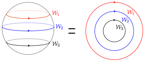
Figure 5: Multiple 1/8181/8-BPS loops with the same orientations. The left figure is a configuration drawn on S2superscript𝑆2S^{2} while the right figure is the same configuration viewed from the south pole and projected to a plane. We denote the area inside 𝒲jsubscript𝒲𝑗\mathcal{W}_{j} (in the right figure) by Ajsubscript𝐴𝑗A_{j}.

Carrying out the same analysis for correlators of more than two Wilson loops of the same orientations (see figure 5 for details of the setup), we obtain a simple generalization of (2.46),

j=1n𝒲j=𝒞1𝒞nj=1ndujfAj(uj)8π2g2j<kΔ¯(uj,uk)M.delimited-⟨⟩superscriptsubscriptproduct𝑗1𝑛subscript𝒲𝑗subscriptdelimited-⟨⟩subscriptcontour-integralprecedessubscript𝒞1precedessubscript𝒞𝑛superscriptsubscriptproduct𝑗1𝑛𝑑subscript𝑢𝑗subscript𝑓subscript𝐴𝑗subscript𝑢𝑗8superscript𝜋2superscript𝑔2subscriptproduct𝑗𝑘¯Δsubscript𝑢𝑗subscript𝑢𝑘𝑀\left<\prod_{j=1}^{n}\mathcal{W}_{j}\right>=\left<\oint_{\mathcal{C}_{1}\prec\cdots\prec\mathcal{C}_{n}}\prod_{j=1}^{n}\frac{du_{j}f_{A_{j}}(u_{j})}{8\pi^{2}g^{2}}\prod_{j<k}\bar{\Delta}(u_{j},u_{k})\right>_{M}\,. (2.47)

Interestingly this integral resembles multiparticle integrals [31, 32, 33, 34, 35, 36, 37, 38, 39, 40, 41] in the hexagon approach to the correlation functions and we will use this connection in our upcoming paper [30] to analyze the defect CFT correlators on the higher-rank Wilson loop.

3 Loop Equation and Intersecting Wilson Loops

We now discuss intersecting 1/8181/8 BPS Wilson loops. In section 3.1, we review the derivation of the loop equation in 2d YM in [5]. We then apply it to the results in the previous section and derive integral representations for the intersecting BPS Wilson loops in section 3.2.

Let us make a remark before we proceed: Below we consider the Wilson loops without the normalization factor 1/N1𝑁1/N since they are often more convenient for analyzing the loop equation. To distinguish them from a more standard definition (2.2), we will put a tilde as

𝒲~𝒞:=trPei𝒞Aμ𝑑yμ.assignsubscript~𝒲𝒞trPsuperscript𝑒𝑖subscriptcontour-integral𝒞subscript𝐴𝜇differential-dsuperscript𝑦𝜇\tilde{\mathcal{W}}_{\mathcal{C}}:={\rm tr}{\rm P}e^{i\oint_{\mathcal{C}}A_{\mu}dy^{\mu}}\,. (3.1)

3.1 Review of loop equation in 2d YM

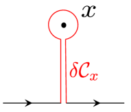
We consider an infinitesimal deformation of the contour 𝒞𝒞+δ𝒞x𝒞𝒞𝛿subscript𝒞𝑥\mathcal{C}\to\mathcal{C}+\delta\mathcal{C}_{x}. Specifically, we pick a point x𝑥x close to but not on top of the Wilson loop. We then add a small circle around x𝑥x and connect it the original contour as depicted in figure 6. This defines the area derivative

δ𝒲~𝒞δσμν(x):=limδσμν0𝒲~𝒞+δ𝒞x𝒲~𝒞δσμν.assign𝛿delimited-⟨⟩subscript~𝒲𝒞𝛿superscript𝜎𝜇𝜈𝑥subscript𝛿superscript𝜎𝜇𝜈0delimited-⟨⟩subscript~𝒲𝒞𝛿subscript𝒞𝑥delimited-⟨⟩subscript~𝒲𝒞𝛿superscript𝜎𝜇𝜈\frac{\delta\langle\tilde{\mathcal{W}}_{\mathcal{C}}\rangle}{\delta\sigma^{\mu\nu}(x)}:=\lim_{\delta\sigma^{\mu\nu}\to 0}\frac{\langle\tilde{\mathcal{W}}_{\mathcal{C}+\delta\mathcal{C}_{x}}\rangle-\langle\tilde{\mathcal{W}}_{\mathcal{C}}\rangle}{\delta\sigma^{\mu\nu}}\,. (3.2)

Here δσμν𝛿superscript𝜎𝜇𝜈\delta\sigma^{\mu\nu} is an area tensor of δ𝒞x𝛿subscript𝒞𝑥\delta\mathcal{C}_{x}, which is a product of the area |δσ|𝛿𝜎|\delta\sigma| and the orientation tensor nμνsuperscript𝑛𝜇𝜈n^{\mu\nu}:

δσμν:=|δσ|nμν.assign𝛿superscript𝜎𝜇𝜈𝛿𝜎superscript𝑛𝜇𝜈\delta\sigma^{\mu\nu}:=|\delta\sigma|n^{\mu\nu}\,. (3.3)

The orientation tensor is unit-normalized and parameterizes the orientation of δ𝒞x𝛿subscript𝒞𝑥\delta\mathcal{C}_{x},

12nμνnμν=1,|δσ|=12nμνδσμν.formulae-sequence12subscript𝑛𝜇𝜈superscript𝑛𝜇𝜈1𝛿𝜎12subscript𝑛𝜇𝜈𝛿superscript𝜎𝜇𝜈\frac{1}{2}n_{\mu\nu}n^{\mu\nu}=1\,,\qquad|\delta\sigma|=\frac{1}{2}n_{\mu\nu}\delta\sigma^{\mu\nu}\,. (3.4)
Refer to caption

(a)𝑎(a)

Refer to caption

(b)𝑏(b)

Figure 6: (a)𝑎(a) Deformation of the contour δ𝒞x𝛿subscript𝒞𝑥\delta\mathcal{C}_{x} denoted in red. We pick a point x𝑥x close to the Wilson loop, draw a small circle and connect it to the original contour. (b)𝑏(b) One-loop correction to 𝚂𝚢𝚖delimited-⟨⟩𝚂𝚢𝚖\langle{\tt Sym}\rangle coming from the gluon exchange. Here we used the double-line notation to make manifest the contraction of indices.

We then expand the path-ordered exponential to get

𝒲~𝒞+δ𝒞x𝒲~𝒞=trP[(eδ𝒞xiAμ𝑑yμ1)e𝒞iAμ𝑑yμ]delimited-⟨⟩subscript~𝒲𝒞𝛿subscript𝒞𝑥delimited-⟨⟩subscript~𝒲𝒞delimited-⟨⟩trPdelimited-[]superscript𝑒subscriptcontour-integral𝛿subscript𝒞𝑥𝑖subscript𝐴𝜇differential-dsuperscript𝑦𝜇1superscript𝑒subscriptcontour-integral𝒞𝑖subscript𝐴𝜇differential-dsuperscript𝑦𝜇\displaystyle\langle\tilde{\mathcal{W}}_{\mathcal{C}+\delta\mathcal{C}_{x}}\rangle-\langle\tilde{\mathcal{W}}_{\mathcal{C}}\rangle=\left<{\rm tr}{\rm P}\left[\left(e^{\oint_{\delta\mathcal{C}_{x}}iA_{\mu}dy^{\mu}}-1\right)e^{\oint_{\mathcal{C}}iA_{\mu}dy^{\mu}}\right]\right> (3.5)
=trP[(δ𝒞xiAμ𝑑yμ12δ𝒞x×δ𝒞xAμ(y1)Aν(y2)𝑑y1μ𝑑y2ν+)e𝒞iAμ𝑑yμ]absentdelimited-⟨⟩trPdelimited-[]subscriptcontour-integral𝛿subscript𝒞𝑥𝑖subscript𝐴𝜇differential-dsuperscript𝑦𝜇12subscriptcontour-integral𝛿subscript𝒞𝑥𝛿subscript𝒞𝑥subscript𝐴𝜇subscript𝑦1subscript𝐴𝜈subscript𝑦2differential-dsuperscriptsubscript𝑦1𝜇differential-dsuperscriptsubscript𝑦2𝜈superscript𝑒subscriptcontour-integral𝒞𝑖subscript𝐴𝜇differential-dsuperscript𝑦𝜇\displaystyle=\left<{\rm tr}{\rm P}\left[\left(\oint_{\delta\mathcal{C}_{x}}iA_{\mu}dy^{\mu}-\frac{1}{2}\oint_{\begin{subarray}{c}\delta\mathcal{C}_{x}\times\delta\mathcal{C}_{x}\end{subarray}}A_{\mu}(y_{1})A_{\nu}(y_{2})dy_{1}^{\mu}dy_{2}^{\nu}+\cdots\right)e^{\oint_{\mathcal{C}}iA_{\mu}dy^{\mu}}\right]\right>

To proceed, we use the Stokes theorem to the first term and write

δ𝒞xiAμ𝑑yμ=i(μAν(x)νAμ(x))2δσμν.subscriptcontour-integral𝛿subscript𝒞𝑥𝑖subscript𝐴𝜇differential-dsuperscript𝑦𝜇𝑖subscript𝜇subscript𝐴𝜈𝑥subscript𝜈subscript𝐴𝜇𝑥2𝛿superscript𝜎𝜇𝜈\oint_{\delta\mathcal{C}_{x}}iA_{\mu}dy^{\mu}=\frac{i\left(\partial_{\mu}A_{\nu}(x)-\partial_{\nu}A_{\mu}(x)\right)}{2}\delta\sigma^{\mu\nu}\,. (3.6)

For the second term, we split it into the symmetric and the antisymmetric parts

P(12δ𝒞x×δ𝒞xAμ(y1)Aν(y2)𝑑y1μ𝑑y2ν)=P12subscriptcontour-integral𝛿subscript𝒞𝑥𝛿subscript𝒞𝑥subscript𝐴𝜇subscript𝑦1subscript𝐴𝜈subscript𝑦2differential-dsuperscriptsubscript𝑦1𝜇differential-dsuperscriptsubscript𝑦2𝜈absent\displaystyle-{\rm P}\left(\frac{1}{2}\oint_{\begin{subarray}{c}\delta\mathcal{C}_{x}\times\delta\mathcal{C}_{x}\end{subarray}}A_{\mu}(y_{1})A_{\nu}(y_{2})dy_{1}^{\mu}dy_{2}^{\nu}\right)= (3.7)
12(δ𝒞xAμ(x)𝑑xμ)2𝚂𝚢𝚖12δ𝒞x×δ𝒞xy1>y2[Aμ(y1),Aν(y2)]𝑑y1μ𝑑y2ν𝙰𝚜𝚢𝚖.subscript12superscriptsubscriptcontour-integral𝛿subscript𝒞𝑥subscript𝐴𝜇𝑥differential-dsuperscript𝑥𝜇2𝚂𝚢𝚖subscript12subscriptcontour-integral𝛿subscript𝒞𝑥𝛿subscript𝒞𝑥subscript𝑦1subscript𝑦2subscript𝐴𝜇subscript𝑦1subscript𝐴𝜈subscript𝑦2differential-dsuperscriptsubscript𝑦1𝜇differential-dsuperscriptsubscript𝑦2𝜈𝙰𝚜𝚢𝚖\displaystyle\underbrace{-\frac{1}{2}\left(\oint_{\delta\mathcal{C}_{x}}A_{\mu}(x)dx^{\mu}\right)^{2}}_{\tt Sym}\underbrace{-\frac{1}{2}\oint_{\begin{subarray}{c}\delta\mathcal{C}_{x}\times\delta\mathcal{C}_{x}\\ y_{1}>y_{2}\end{subarray}}[A_{\mu}(y_{1}),A_{\nu}(y_{2})]dy_{1}^{\mu}dy_{2}^{\nu}}_{\tt Asym}\,.

Here y1>y2subscript𝑦1subscript𝑦2y_{1}>y_{2} means that the integral is path-ordered and y2subscript𝑦2y_{2} is always behind y1subscript𝑦1y_{1}. Since δ𝒞x𝛿subscript𝒞𝑥\delta\mathcal{C}_{x} is an infinitesimal contour around x𝑥x, the antisymmetric part can be approximated as

𝙰𝚜𝚢𝚖𝙰𝚜𝚢𝚖\displaystyle{\tt Asym} [Aμ(x),Aν(x)]2δ𝒞x×δ𝒞xy1>y2𝑑y1μ𝑑y2νsimilar-to-or-equalsabsentsubscript𝐴𝜇𝑥subscript𝐴𝜈𝑥2subscriptcontour-integral𝛿subscript𝒞𝑥𝛿subscript𝒞𝑥subscript𝑦1subscript𝑦2differential-dsuperscriptsubscript𝑦1𝜇differential-dsuperscriptsubscript𝑦2𝜈\displaystyle\simeq-\frac{[A_{\mu}(x),A_{\nu}(x)]}{2}\oint_{\begin{subarray}{c}\delta\mathcal{C}_{x}\times\delta\mathcal{C}_{x}\\ y_{1}>y_{2}\end{subarray}}dy_{1}^{\mu}dy_{2}^{\nu} (3.8)
=[Aμ(y),Aν(y)]2δ𝒞xy2μ𝑑y2ν=[Aμ(x),Aν(x)]2δσμν.absentsubscript𝐴𝜇𝑦subscript𝐴𝜈𝑦2subscriptcontour-integral𝛿subscript𝒞𝑥superscriptsubscript𝑦2𝜇differential-dsuperscriptsubscript𝑦2𝜈subscript𝐴𝜇𝑥subscript𝐴𝜈𝑥2𝛿superscript𝜎𝜇𝜈\displaystyle=\frac{[A_{\mu}(y),A_{\nu}(y)]}{2}\oint_{\delta\mathcal{C}_{x}}y_{2}^{\mu}dy_{2}^{\nu}=\frac{[A_{\mu}(x),A_{\nu}(x)]}{2}\delta\sigma^{\mu\nu}\,.

The sum of (3.6) and (3.8) gives iFμν(y)/2𝑖subscript𝐹𝜇𝜈𝑦2iF_{\mu\nu}(y)/2 with Fμν=μAνμAνi[Aμ,Aν]subscript𝐹𝜇𝜈subscript𝜇subscript𝐴𝜈subscript𝜇subscript𝐴𝜈𝑖subscript𝐴𝜇subscript𝐴𝜈F_{\mu\nu}=\partial_{\mu}A_{\nu}-\partial_{\mu}A_{\nu}-i[A_{\mu},A_{\nu}].

On the other hand, the symmetric part at one loop reads (see figure 6)

𝚂𝚢𝚖|1-loopevaluated-atdelimited-⟨⟩𝚂𝚢𝚖1-loop\displaystyle\left.\langle{\tt Sym}\rangle\right|_{\text{1-loop}} =N2δCx𝑑y1μδCx𝑑y2νGμν(y1y2)×𝟏absent𝑁2subscriptcontour-integral𝛿subscript𝐶𝑥differential-dsuperscriptsubscript𝑦1𝜇subscriptcontour-integral𝛿subscript𝐶𝑥differential-dsuperscriptsubscript𝑦2𝜈subscript𝐺𝜇𝜈subscript𝑦1subscript𝑦21\displaystyle=-\frac{N}{2}\oint_{\delta C_{x}}dy_{1}^{\mu}\oint_{\delta C_{x}}dy_{2}^{\nu}G_{\mu\nu}(y_{1}-y_{2})\times{\bf 1} (3.9)

Here 𝟏1{\bf 1} is the identity matrix for the color factors and Gμν(x1x2)subscript𝐺𝜇𝜈subscript𝑥1subscript𝑥2G_{\mu\nu}(x_{1}-x_{2}) is a propagator of gauge fields without color factors. In the axial gauge (A1=0subscript𝐴10A_{1}=0), it reads444Note that our normalization for the coupling constant in 2d YM is different from [5]: (g2d[5])2=(g2dours)2/2superscriptsuperscriptsubscript𝑔2d[5]2superscriptsubscriptsuperscript𝑔ours2d22(g_{\rm 2d}^{\text{\cite[cite]{[\@@bibref{}{Kazakov:1980zi}{}{}]}}})^{2}=(g^{\rm ours}_{\rm 2d})^{2}/2.

Gμν(xy)=δμ2δν2g2d24δ(x2y2)|x1y1|.subscript𝐺𝜇𝜈𝑥𝑦subscriptsuperscript𝛿2𝜇subscriptsuperscript𝛿2𝜈superscriptsubscript𝑔2d24𝛿superscript𝑥2superscript𝑦2superscript𝑥1superscript𝑦1\displaystyle G_{\mu\nu}(x-y)=-\delta^{2}_{\mu}\delta^{2}_{\nu}\frac{g_{\rm 2d}^{2}}{4}\delta(x^{2}-y^{2})|x^{1}-y^{1}|\,. (3.10)

Plugging this into (3.9), we get

𝚂𝚢𝚖|1-loop=g2d2N4|δσ|.evaluated-atdelimited-⟨⟩𝚂𝚢𝚖1-loopsuperscriptsubscript𝑔2d2𝑁4𝛿𝜎\left.\langle{\tt Sym}\rangle\right|_{\text{1-loop}}=-\frac{g_{\rm 2d}^{2}N}{4}|\delta\sigma|\,. (3.11)

A couple of comments are in order: First, the result (3.9) receives higher loop corrections. However since g2dsubscript𝑔2dg_{\rm 2d} has mass dimension 111, it follows from dimensional analysis that the loop corrections come with higher powers of δσμν𝛿superscript𝜎𝜇𝜈\delta\sigma^{\mu\nu} and therefore can be neglected in the small area limit δσμν0𝛿superscript𝜎𝜇𝜈0\delta\sigma^{\mu\nu}\to 0. Second, although (3.11) was computed in a specific gauge, the result is actually gauge-invariant. This is because the tree-level555As stated above, the higher-loop corrections can be neglected in the small area limit. gauge transformation

Aμ(y)Aμ(y)+μα(y),subscript𝐴𝜇𝑦maps-tosubscript𝐴𝜇𝑦subscript𝜇𝛼𝑦A_{\mu}(y)\quad\mapsto\quad A_{\mu}(y)+\partial_{\mu}\alpha(y)\,, (3.12)

only changes (3.9) by a term that integrates to zero:

δ𝚂𝚢𝚖δ𝒞x𝑑y1μμα(y1)δ𝒞x𝑑y2ννα(y2)=0.proportional-to𝛿𝚂𝚢𝚖subscriptcontour-integral𝛿subscript𝒞𝑥differential-dsuperscriptsubscript𝑦1𝜇subscript𝜇𝛼subscript𝑦1subscriptcontour-integral𝛿subscript𝒞𝑥differential-dsuperscriptsubscript𝑦2𝜈subscript𝜈𝛼subscript𝑦20\delta{\tt Sym}\propto\oint_{\delta\mathcal{C}_{x}}dy_{1}^{\mu}\partial_{\mu}\alpha(y_{1})\oint_{\delta\mathcal{C}_{x}}dy_{2}^{\nu}\partial_{\nu}\alpha(y_{2})=0\,. (3.13)

Third, the result (3.9) is for the U(N)𝑁(N) gauge group and the answer will be different for other gauge groups. It would be interesting to derive the loop equation for general gauge groups.

Now, combining the symmetric and antisymmetric parts, we arrive at the following expression for the first-order variation:

δ𝒲~𝒞δσμν(x)=trP[iFμν(x)e𝒞iAμ𝑑yμ]g2d2N4nμν(x)𝒲~𝒞.𝛿delimited-⟨⟩subscript~𝒲𝒞𝛿superscript𝜎𝜇𝜈𝑥delimited-⟨⟩trPdelimited-[]𝑖subscript𝐹𝜇𝜈𝑥superscript𝑒subscriptcontour-integral𝒞𝑖subscript𝐴𝜇differential-dsuperscript𝑦𝜇superscriptsubscript𝑔2d2𝑁4subscript𝑛𝜇𝜈𝑥delimited-⟨⟩subscript~𝒲𝒞\displaystyle\frac{\delta\langle\tilde{\mathcal{W}}_{\mathcal{C}}\rangle}{\delta\sigma^{\mu\nu}(x)}=\left<{\rm tr}{\rm P}\left[iF_{\mu\nu}(x)e^{\oint_{\mathcal{C}}iA_{\mu}dy^{\mu}}\right]\right>-\frac{g_{\rm 2d}^{2}N}{4}n_{\mu\nu}(x)\langle\tilde{\mathcal{W}}_{\mathcal{C}}\rangle\,. (3.14)

Let us make some clarification on the second term in (3.14): First, it contains the orientation tensor nμνsubscript𝑛𝜇𝜈n_{\mu\nu} and changes discontinuously across the contour. This property plays a crucial role in the derivation below. Second, it may appear to contradict a familar statement that the small deformation of the Wilson loop is simply given by the insertion of Fμνsubscript𝐹𝜇𝜈F_{\mu\nu}. This apparent contradiction comes from the difference of the regularizations: Normally we insert Fμνsubscript𝐹𝜇𝜈F_{\mu\nu} on top of the Wilson loop and regularize divergent diagrams which contract Fμνsubscript𝐹𝜇𝜈F_{\mu\nu} and the loop by the principal value prescription. On the other hand, Fμνsubscript𝐹𝜇𝜈F_{\mu\nu} in (3.14) is inserted slightly above or below the loop, which gives a different regularization. This alternative regularization produces a different answer, but one can show by the explicit computation666In the holomorphic gauge Az¯=0subscript𝐴¯𝑧0A_{\bar{z}}=0, the contraction of Fμνsubscript𝐹𝜇𝜈F_{\mu\nu} and the straight-line loop reads (see e.g. [23]) 𝑑yiFzz¯(x)iAz(y)=g2d2N4π𝑑yi1+y21+xyxy.superscriptsubscriptdifferential-d𝑦delimited-⟨⟩𝑖subscript𝐹𝑧¯𝑧𝑥𝑖subscript𝐴𝑧𝑦superscriptsubscript𝑔2d2𝑁4𝜋superscriptsubscriptdifferential-d𝑦𝑖1superscript𝑦21𝑥𝑦𝑥𝑦\int_{-\infty}^{\infty}dy\langle i\ast F_{z\bar{z}}(x)iA_{z}(y)\rangle=-\frac{g_{\rm 2d}^{2}N}{4\pi}\int_{-\infty}^{\infty}dy\frac{i}{1+y^{2}}\frac{1+xy}{x-y}\,. (3.15) In the principal value prescription, this integral vanishes while if we shift x𝑥x slightly above or below by adding ±iϵplus-or-minus𝑖italic-ϵ\pm i\epsilon, it gives ±g2d2N/(4π)plus-or-minussuperscriptsubscript𝑔2d2𝑁4𝜋\pm g_{\rm 2d}^{2}N/(4\pi), which are precisely canceled by the second term in (3.14). that the sum of the two terms in (3.14) reproduces the result in the principal value prescription. We thus have

δ𝒲~𝒞δσμν(x)=trP[iFμν(x)e𝒞iAμ𝑑yμ]|principal value,𝛿delimited-⟨⟩subscript~𝒲𝒞𝛿superscript𝜎𝜇𝜈𝑥evaluated-atdelimited-⟨⟩trPdelimited-[]𝑖subscript𝐹𝜇𝜈𝑥superscript𝑒subscriptcontour-integral𝒞𝑖subscript𝐴𝜇differential-dsuperscript𝑦𝜇principal value\frac{\delta\langle\tilde{\mathcal{W}}_{\mathcal{C}}\rangle}{\delta\sigma^{\mu\nu}(x)}=\left.\left<{\rm tr}{\rm P}\left[iF_{\mu\nu}(x)e^{\oint_{\mathcal{C}}iA_{\mu}dy^{\mu}}\right]\right>\right|_{\text{principal value}}\,, (3.16)

which is consistent with the familiar statement.

Now we derive the loop equation. First we differentiate (3.14) and get

μδW~𝒞δσμν(x)=trP[iμFμν(x)e𝒞iAμ𝑑yμ]g2d2N4μnμν(x)𝒲~𝒞.superscript𝜇𝛿delimited-⟨⟩subscript~𝑊𝒞𝛿superscript𝜎𝜇𝜈𝑥delimited-⟨⟩trPdelimited-[]𝑖superscript𝜇subscript𝐹𝜇𝜈𝑥superscript𝑒subscriptcontour-integral𝒞𝑖subscript𝐴𝜇differential-dsuperscript𝑦𝜇superscriptsubscript𝑔2d2𝑁4superscript𝜇subscript𝑛𝜇𝜈𝑥delimited-⟨⟩subscript~𝒲𝒞\partial^{\mu}\frac{\delta\langle\tilde{W}_{\mathcal{C}}\rangle}{\delta\sigma^{\mu\nu}(x)}=\left<{\rm tr}{\rm P}\left[i\nabla^{\mu}F_{\mu\nu}(x)e^{\oint_{\mathcal{C}}iA_{\mu}dy^{\mu}}\right]\right>-\frac{g_{\rm 2d}^{2}N}{4}\partial^{\mu}n_{\mu\nu}(x)\langle\tilde{\mathcal{W}}_{\mathcal{C}}\rangle\,. (3.17)

To evaluate μnμνsuperscript𝜇subscript𝑛𝜇𝜈\partial^{\mu}n_{\mu\nu} that appears in the second term, it is useful to go back to the definition

μδW~𝒞δσμν(x):=limε01ε(δ𝒲~𝒞δσμν(x+ϵμ/2)δ𝒲~𝒞δσμν(xϵμ/2)).assignsuperscript𝜇𝛿delimited-⟨⟩subscript~𝑊𝒞𝛿superscript𝜎𝜇𝜈𝑥subscript𝜀01𝜀𝛿delimited-⟨⟩subscript~𝒲𝒞𝛿superscript𝜎𝜇𝜈𝑥subscriptitalic-ϵ𝜇2𝛿delimited-⟨⟩subscript~𝒲𝒞𝛿superscript𝜎𝜇𝜈𝑥subscriptitalic-ϵ𝜇2\partial^{\mu}\frac{\delta\langle\tilde{W}_{\mathcal{C}}\rangle}{\delta\sigma^{\mu\nu}(x)}:=\lim_{\varepsilon\to 0}\frac{1}{\varepsilon}\left(\frac{\delta\langle\tilde{\mathcal{W}}_{\mathcal{C}}\rangle}{\delta\sigma^{\mu\nu}(x+\epsilon_{\mu}/2)}-\frac{\delta\langle\tilde{\mathcal{W}}_{\mathcal{C}}\rangle}{\delta\sigma^{\mu\nu}(x-\epsilon_{\mu}/2)}\right)\,. (3.18)

Here we take x𝑥x to be a point on the Wilson loop and ϵμsubscriptitalic-ϵ𝜇\epsilon_{\mu} to be a vector of length ε𝜀\varepsilon in the μ𝜇\mu direction; (ϵμ)ρ:=εδμρassignsuperscriptsubscriptitalic-ϵ𝜇𝜌𝜀subscriptsuperscript𝛿𝜌𝜇\left(\epsilon_{\mu}\right)^{\rho}:=\varepsilon\delta^{\rho}_{\mu}. Since the points x±ϵμ/2plus-or-minus𝑥subscriptitalic-ϵ𝜇2x\pm\epsilon_{\mu}/2 sit on different sides of the loop, we have nμν(x±ϵμ/2)=±1subscript𝑛𝜇𝜈plus-or-minus𝑥subscriptitalic-ϵ𝜇2plus-or-minus1n_{\mu\nu}(x\pm\epsilon_{\mu}/2)=\pm 1. Thus the derivative μnμνsuperscript𝜇subscript𝑛𝜇𝜈\partial^{\mu}n_{\mu\nu} picks up a contribution from a delta function

μnμν(x)=2Ix𝑑xνδ(2)(xx),superscript𝜇subscript𝑛𝜇𝜈𝑥2subscriptsubscript𝐼𝑥differential-dsubscriptsuperscript𝑥𝜈superscript𝛿2superscript𝑥𝑥\partial^{\mu}n_{\mu\nu}(x)=2\int_{I_{x}}dx^{\prime}_{\nu}\,\delta^{(2)}(x^{\prime}-x)\,, (3.19)

where the contour Ixsubscript𝐼𝑥I_{x} is an infinitesimal one-dimensional segment which passes through x𝑥x. Second we use the fact that μFμνsuperscript𝜇subscript𝐹𝜇𝜈\nabla^{\mu}F_{\mu\nu} is proportional to the equation of motion777S2dsubscript𝑆2dS_{\text{2d}} is the Euclidean action for 2d YM given by (2.4).

μFμν=g2d22δS2dδAν.superscript𝜇subscript𝐹𝜇𝜈superscriptsubscript𝑔2d22𝛿subscript𝑆2d𝛿superscript𝐴𝜈\nabla^{\mu}F_{\mu\nu}=-\frac{g_{\text{2d}}^{2}}{2}\frac{\delta S_{\text{2d}}}{\delta A^{\nu}}\,. (3.20)

We can then replace it inside the expectation value as

<(μFμν(x))ab>g2d22δδ(Aν(x))ba().\Big{<}\left(\nabla^{\mu}F_{\mu\nu}(x)\right)^{a}{}_{b}\cdots\Big{>}\mapsto-\frac{g_{\text{2d}}^{2}}{2}\left<\frac{\delta}{\delta\left(A^{\nu}(x)\right)^{b}{}_{a}}\left(\cdots\right)\right>\,. (3.21)

Here we wrote the gauge indices a𝑎a and b𝑏b explicitly for convenience. As a result we get (see also figure 7)

trP[iμFμν(x)e𝒞iAμ𝑑yμ]=ig2d22δδ(Aν(x))ba[Pe𝒞iAμ𝑑yμ]ba\displaystyle\left<{\rm tr}{\rm P}\left[i\nabla^{\mu}F_{\mu\nu}(x)e^{\oint_{\mathcal{C}}iA_{\mu}dy^{\mu}}\right]\right>=-i\frac{g_{\rm 2d}^{2}}{2}\left<\frac{\delta}{\delta\left(A^{\nu}(x)\right)^{b}{}_{a}}\left[{\rm P}e^{\oint_{\mathcal{C}}iA_{\mu}dy^{\mu}}\right]^{b}{}_{a}\right> (3.22)
=g2d22𝒞𝑑xνδ(2)(xx)trP[exxiAμ𝑑yμ]trP[exxiAμ𝑑yμ].absentsuperscriptsubscript𝑔2d22subscriptcontour-integral𝒞differential-dsubscriptsuperscript𝑥𝜈superscript𝛿2superscript𝑥𝑥delimited-⟨⟩trPdelimited-[]superscript𝑒superscriptsubscriptcontour-integral𝑥superscript𝑥𝑖subscript𝐴𝜇differential-dsuperscript𝑦𝜇trPdelimited-[]superscript𝑒superscriptsubscriptcontour-integralsuperscript𝑥𝑥𝑖subscript𝐴𝜇differential-dsuperscript𝑦𝜇\displaystyle=\frac{g_{\rm 2d}^{2}}{2}\oint_{\mathcal{C}}dx^{\prime}_{\nu}\,\,\delta^{(2)}(x^{\prime}-x)\left<{\rm tr}{\rm P}\left[e^{\oint_{x}^{x^{\prime}}iA_{\mu}dy^{\mu}}\right]{\rm tr}{\rm P}\left[e^{\oint_{x^{\prime}}^{x}iA_{\mu}dy^{\mu}}\right]\right>\,.
Refer to caption
Figure 7: The Ward identity on the Wilson loop. The insertion of μFμνsuperscript𝜇subscript𝐹𝜇𝜈\nabla^{\mu}F_{\mu\nu} on the loop can be replaced with the functional derivative δ/δAν𝛿𝛿subscript𝐴𝜈\delta/\delta A_{\nu}. When it acts on other parts of the contour, it cuts the loop and reconnects it as shown in the figure.

The integral (3.22) is nonzero even for nonintersecting Wilson loops since it receives a contribution from a “self contraction”, namely a contribution from a trivial coincidence point x=xsuperscript𝑥𝑥x^{\prime}=x on the loop. It can be evaluated as

(self-contraction)self-contraction\displaystyle\left(\text{self-contraction}\right) =g2d22Ix𝑑xνδ(2)(xx)trP[e𝒞iAμ𝑑yμ]tr[𝟏]absentsuperscriptsubscript𝑔2d22subscriptsubscript𝐼𝑥differential-dsubscriptsuperscript𝑥𝜈superscript𝛿2superscript𝑥𝑥delimited-⟨⟩trPdelimited-[]superscript𝑒subscriptcontour-integral𝒞𝑖subscript𝐴𝜇differential-dsuperscript𝑦𝜇trdelimited-[]1\displaystyle=\frac{g_{\rm 2d}^{2}}{2}\int_{I_{x}}dx^{\prime}_{\nu}\delta^{(2)}(x^{\prime}-x)\left<{\rm tr}{\rm P}\left[e^{\oint_{\mathcal{C}}iA_{\mu}dy^{\mu}}\right]{\rm tr}\left[{\bf 1}\right]\right> (3.23)
=g2d2N2Ix𝑑xνδ(2)(xx)trP[e𝒞iAμ𝑑yμ].absentsuperscriptsubscript𝑔2d2𝑁2subscriptsubscript𝐼𝑥differential-dsubscriptsuperscript𝑥𝜈superscript𝛿2superscript𝑥𝑥delimited-⟨⟩trPdelimited-[]superscript𝑒subscriptcontour-integral𝒞𝑖subscript𝐴𝜇differential-dsuperscript𝑦𝜇\displaystyle=\frac{g_{\rm 2d}^{2}N}{2}\int_{I_{x}}dx^{\prime}_{\nu}\,\delta^{(2)}(x^{\prime}-x)\left<{\rm tr}{\rm P}\left[e^{\oint_{\mathcal{C}}iA_{\mu}dy^{\mu}}\right]\right>\,.

As can be seen from (3.19), this turns out to cancel the second term in (3.17). Thus, when the two terms in (3.17) are combined, we are left with contributions only from intersecting points and obtain the loop equation

μδW~𝒞δσμν(x)=g2d22𝒞𝑑xνδ(2)(xx)trP[exxiAμ𝑑yμ]trP[exxiAμ𝑑yμ],superscript𝜇𝛿delimited-⟨⟩subscript~𝑊𝒞𝛿superscript𝜎𝜇𝜈𝑥superscriptsubscript𝑔2d22subscript𝒞differential-dsubscriptsuperscript𝑥𝜈superscript𝛿2superscript𝑥𝑥delimited-⟨⟩trPdelimited-[]superscript𝑒superscriptsubscriptcontour-integral𝑥superscript𝑥𝑖subscript𝐴𝜇differential-dsuperscript𝑦𝜇trPdelimited-[]superscript𝑒superscriptsubscriptcontour-integralsuperscript𝑥𝑥𝑖subscript𝐴𝜇differential-dsuperscript𝑦𝜇\partial^{\mu}\frac{\delta\langle\tilde{W}_{\mathcal{C}}\rangle}{\delta\sigma^{\mu\nu}(x)}=\frac{g_{\rm 2d}^{2}}{2}{{\rm-}\!\!\!\!\!\!\int_{\mathcal{C}}}dx^{\prime}_{\nu}\,\,\delta^{(2)}(x^{\prime}-x)\left<{\rm tr}{\rm P}\left[e^{\oint_{x}^{x^{\prime}}iA_{\mu}dy^{\mu}}\right]{\rm tr}{\rm P}\left[e^{\oint_{x^{\prime}}^{x}iA_{\mu}dy^{\mu}}\right]\right>\,, (3.24)

where the symbol 𝒞subscript𝒞{\rm-}\!\!\!\!\!\int_{\mathcal{C}} means that we remove an infinitesimal segment around x𝑥x when we perform the integral. For the actual application, it is useful to choose ν𝜈\nu to be the direction of the Wilson loop near the intersection and μ𝜇\mu to be the direction orthogonal to it. In addition, we integrate (3.24) along a small path in the μ𝜇\mu direction. For the left hand side, this is basically equivalent to going back to the definition (3.18) and removing 1/ε1𝜀1/\varepsilon, which can be pictorially represented as888In the last equality, we used δσμν(x+ϵμ/2)=δσμν(xϵμ/2)=|δσ|𝛿superscript𝜎𝜇𝜈𝑥subscriptitalic-ϵ𝜇2𝛿superscript𝜎𝜇𝜈𝑥subscriptitalic-ϵ𝜇2𝛿𝜎\delta\sigma^{\mu\nu}(x+\epsilon_{\mu}/2)=-\delta\sigma^{\mu\nu}(x-\epsilon_{\mu}/2)=|\delta\sigma|.

L^x𝒲~𝒞:=limε0δ𝒲~𝒞δσμν(x+ϵμ/2)δ𝒲~𝒞δσμν(xϵμ/2)assignsubscript^𝐿𝑥delimited-⟨⟩subscript~𝒲𝒞subscript𝜀0𝛿delimited-⟨⟩subscript~𝒲𝒞𝛿superscript𝜎𝜇𝜈𝑥subscriptitalic-ϵ𝜇2𝛿delimited-⟨⟩subscript~𝒲𝒞𝛿superscript𝜎𝜇𝜈𝑥subscriptitalic-ϵ𝜇2\displaystyle\hat{L}_{x}\langle\tilde{\mathcal{W}}_{\mathcal{C}}\rangle:=\lim_{\varepsilon\to 0}\frac{\delta\langle\tilde{\mathcal{W}}_{\mathcal{C}}\rangle}{\delta\sigma^{\mu\nu}(x+\epsilon_{\mu}/2)}-\frac{\delta\langle\tilde{\mathcal{W}}_{\mathcal{C}}\rangle}{\delta\sigma^{\mu\nu}(x-\epsilon_{\mu}/2)}
=1δσμν(x+ϵμ2)([Uncaptioned image][Uncaptioned image])1δσμν(xϵμ2)([Uncaptioned image][Uncaptioned image])absent1𝛿superscript𝜎𝜇𝜈𝑥subscriptitalic-ϵ𝜇2[Uncaptioned image][Uncaptioned image]1𝛿superscript𝜎𝜇𝜈𝑥subscriptitalic-ϵ𝜇2[Uncaptioned image][Uncaptioned image]\displaystyle=\frac{1}{\delta\sigma^{\mu\nu}(x+\frac{\epsilon_{\mu}}{2})}\left(\raisebox{-19.91684pt}{\includegraphics[clip,height=42.67912pt]{def1.pdf}}-\raisebox{-19.91684pt}{\includegraphics[clip,height=42.67912pt]{def2.pdf}}\right)-\frac{1}{\delta\sigma^{\mu\nu}(x-\frac{\epsilon_{\mu}}{2})}\left(\raisebox{-19.91684pt}{\includegraphics[clip,height=42.67912pt]{def3.pdf}}-\raisebox{-19.91684pt}{\includegraphics[clip,height=42.67912pt]{def4.pdf}}\right)
=1|δσ|([Uncaptioned image]+[Uncaptioned image]2[Uncaptioned image]).absent1𝛿𝜎[Uncaptioned image][Uncaptioned image]2[Uncaptioned image]\displaystyle=\frac{1}{|\delta\sigma|}\left(\raisebox{-19.91684pt}{\includegraphics[clip,height=42.67912pt]{def1.pdf}}+\raisebox{-19.91684pt}{\includegraphics[clip,height=42.67912pt]{def3.pdf}}-2\raisebox{-19.91684pt}{\includegraphics[clip,height=42.67912pt]{def2.pdf}}\right)\,. (3.25)

We then get

L^x𝒲~𝒞=g2d22𝒲~𝒞1𝒲~𝒞2,subscript^𝐿𝑥delimited-⟨⟩subscript~𝒲𝒞superscriptsubscript𝑔2d22delimited-⟨⟩subscript~𝒲subscript𝒞1subscript~𝒲subscript𝒞2\hat{L}_{x}\langle\tilde{\mathcal{W}}_{\mathcal{C}}\rangle=\frac{g_{\rm 2d}^{2}}{2}\left<\tilde{\mathcal{W}}_{\mathcal{C}_{1}}\tilde{\mathcal{W}}_{\mathcal{C}_{2}}\right>\,, (3.26)

where 𝒞1,2subscript𝒞12\mathcal{C}_{1,2} are the two contours obtained by reconnecting the loop 𝒞𝒞\mathcal{C} at the point x𝑥x. Here we assumed that only two lines intersect at the point x𝑥x. When more than two lines intersect, the right hand side of (3.26) is replaced by a sum of all possible reconnections.

Using the fact that the Wilson loops in 2d YM only depend on the area, we can convert (3.26) to area derivatives (see figure 8),

L^x𝒲~𝒞=(S1+S3S2S4)𝒲~𝒞=g2d22𝒲~𝒞1𝒲~𝒞2.subscript^𝐿𝑥delimited-⟨⟩subscript~𝒲𝒞subscriptsubscript𝑆1subscriptsubscript𝑆3subscriptsubscript𝑆2subscriptsubscript𝑆4delimited-⟨⟩subscript~𝒲𝒞superscriptsubscript𝑔2d22delimited-⟨⟩subscript~𝒲subscript𝒞1subscript~𝒲subscript𝒞2\hat{L}_{x}\langle\tilde{\mathcal{W}}_{\mathcal{C}}\rangle=\left(\partial_{S_{1}}+\partial_{S_{3}}-\partial_{S_{2}}-\partial_{S_{4}}\right)\langle\tilde{\mathcal{W}}_{\mathcal{C}}\rangle=\frac{g_{\rm 2d}^{2}}{2}\left<\tilde{\mathcal{W}}_{\mathcal{C}_{1}}\tilde{\mathcal{W}}_{\mathcal{C}_{2}}\right>\,. (3.27)

This formula can be applied straightforwardly when the loop is on R2superscript𝑅2R^{2}. For loops on S2superscript𝑆2S^{2}, not all the areas (Sisubscript𝑆𝑖S_{i}’s) are independent. In such a case, we go back to the pictorial definition of L^xsubscript^𝐿𝑥\hat{L}_{x} given in (3.25) and translate it into area derivatives as we see in the next subsection.

Refer to caption
Figure 8: The area derivatives and the loop laplacian L^xsubscript^𝐿𝑥\hat{L}_{x}. The left hand side is the definition of L^xsubscript^𝐿𝑥\hat{L}_{x} which can be easily translated into area derivatives. (Adapted from [5].)

3.2 Intersecting BPS loops in 𝒩=4𝒩4\mathcal{N}=4 SYM

We now apply the loop equation (3.27) and compute the expectation value of intersecting 1/8181/8-BPS loops in 𝒩=4𝒩4\mathcal{N}=4 SYM.

3.2.1 Figure eight loop

The simplest intersecting loop is the “figure eight” loop. Since the figure eight loop on S2superscript𝑆2S^{2} is equivalent to a one-intersection loop (see figure 9), we start with the latter, and the result for the figure-eight can be simply obtained by relating the areas as in figure 9.

Under the action of L^xsubscript^𝐿𝑥\hat{L}_{x}, the one-intersection loop 𝒲~A1,A2subscript~𝒲subscript𝐴1subscript𝐴2\tilde{\mathcal{W}}_{A_{1},A_{2}} reconnects to a product of two disconnected loops 𝒲1,2subscript𝒲12\mathcal{W}_{1,2} with areas A1,2subscript𝐴12A_{1,2}. Using (3.25), this can be translated into area derivatives as follows999To derive this, one simply needs to note that the first term (3.25) decreases A2subscript𝐴2A_{2} while the second term increases A1subscript𝐴1A_{1} when applied to the one-intersection loop.:

(A1A2)𝒲~A1,A2=4πg2N𝒲~1𝒲~2.subscriptsubscript𝐴1subscriptsubscript𝐴2delimited-⟨⟩subscript~𝒲subscript𝐴1subscript𝐴24𝜋superscript𝑔2𝑁delimited-⟨⟩subscript~𝒲1subscript~𝒲2(\partial_{A_{1}}-\partial_{A_{2}})\langle\tilde{\mathcal{W}}_{A_{1},A_{2}}\rangle=-\frac{4\pi g^{2}}{N}\langle\tilde{\mathcal{W}}_{1}\tilde{\mathcal{W}}_{2}\rangle\,. (3.28)

Here we rewrote g2dsubscript𝑔2dg_{\rm 2d} in terms of the coupling in 𝒩=4𝒩4\mathcal{N}=4 SYM using (2.3) and (2.16): g2d2=gYM2/(2π)=8πg2/Nsuperscriptsubscript𝑔2d2superscriptsubscript𝑔YM22𝜋8𝜋superscript𝑔2𝑁g_{\rm 2d}^{2}=-g_{\rm YM}^{2}/(2\pi)=-8\pi g^{2}/N. Dividing both sides by N𝑁N, we get the equation for the normalizaed expectation value

(A1A2)𝒲A1,A2=4πg𝒲1𝒲2.subscriptsubscript𝐴1subscriptsubscript𝐴2delimited-⟨⟩subscript𝒲subscript𝐴1subscript𝐴24𝜋𝑔delimited-⟨⟩subscript𝒲1subscript𝒲2(\partial_{A_{1}}-\partial_{A_{2}})\langle\mathcal{W}_{A_{1},A_{2}}\rangle=-4\pi g\langle\mathcal{W}_{1}\mathcal{W}_{2}\rangle\,. (3.29)

This can be solved by replacing the right hand side with the integrals (2.42). The result reads

𝒲A1,A2=delimited-⟨⟩subscript𝒲subscript𝐴1subscript𝐴2absent\displaystyle\langle\mathcal{W}_{A_{1},A_{2}}\rangle= (3.30)
4πg2idu18π2g2du28π2g2Δ¯(u1,u2)fA1(u1)fA2(u2)u1u2+12du8π2g2fA1(u)fA2(uiϵ)M.subscriptdelimited-⟨⟩4𝜋superscript𝑔2𝑖contour-integral𝑑subscript𝑢18superscript𝜋2superscript𝑔2𝑑subscript𝑢28superscript𝜋2superscript𝑔2¯Δsubscript𝑢1subscript𝑢2subscript𝑓subscript𝐴1subscript𝑢1subscript𝑓subscript𝐴2subscript𝑢2subscript𝑢1subscript𝑢212contour-integral𝑑𝑢8superscript𝜋2superscript𝑔2subscript𝑓subscript𝐴1𝑢subscript𝑓subscript𝐴2𝑢𝑖italic-ϵ𝑀\displaystyle\left<4\pi g^{2}i\oint\frac{du_{1}}{8\pi^{2}g^{2}}\frac{du_{2}}{8\pi^{2}g^{2}}\bar{\Delta}(u_{1},u_{2})\frac{f_{A_{1}}(u_{1})f_{A_{2}}(u_{2})}{u_{1}-u_{2}}+\frac{1}{2}\oint\frac{du}{8\pi^{2}g^{2}}f_{A_{1}}(u)f_{A_{2}}(u-i\epsilon)\right>_{M}\,.

Alternatively, one can use (2.46) to write

𝒲A1,A2=4πg2i𝒞1𝒞2du18π2g2du28π2g2Δ¯(u1,u2)fA1(u1)fA2(u2)u1u2M.delimited-⟨⟩subscript𝒲subscript𝐴1subscript𝐴2subscriptdelimited-⟨⟩4𝜋superscript𝑔2𝑖subscriptcontour-integralprecedessubscript𝒞1subscript𝒞2𝑑subscript𝑢18superscript𝜋2superscript𝑔2𝑑subscript𝑢28superscript𝜋2superscript𝑔2¯Δsubscript𝑢1subscript𝑢2subscript𝑓subscript𝐴1subscript𝑢1subscript𝑓subscript𝐴2subscript𝑢2subscript𝑢1subscript𝑢2𝑀\langle\mathcal{W}_{A_{1},A_{2}}\rangle=\left<4\pi g^{2}i\oint_{\mathcal{C}_{1}\prec\mathcal{C}_{2}}\frac{du_{1}}{8\pi^{2}g^{2}}\frac{du_{2}}{8\pi^{2}g^{2}}\bar{\Delta}(u_{1},u_{2})\frac{f_{A_{1}}(u_{1})f_{A_{2}}(u_{2})}{u_{1}-u_{2}}\right>_{M}\,. (3.31)

Translating this to the figure eight loop using the relation (see figure 9),

A1=4πA¯1A2=A¯2,formulae-sequencesubscript𝐴14𝜋subscript¯𝐴1subscript𝐴2subscript¯𝐴2A_{1}=4\pi-\bar{A}_{1}\qquad A_{2}=\bar{A}_{2}\,, (3.32)

we obtain (1.1) in the introduction. A simple consistency check of (3.30) is to consider the special case A2=A1subscript𝐴2subscript𝐴1A_{2}=A_{1}, which yields a doubly-wound fundamental Wilson loop. For A2=A1subscript𝐴2subscript𝐴1A_{2}=A_{1}, the double-integral in (3.30) vanishes due to antisymmetry of the integrand, and the single integral reproduces the expected result for the doubly-wound loop, which is given by (2.26) with gYM2gYMsubscript𝑔YM2subscript𝑔YMg_{\rm YM}\rightarrow 2g_{\rm YM}.101010For a k𝑘k-wound fundamental loop, it is easy to see from the Gaussian matrix model (2.5) that Wkwound=Wsingle|gYMkgYM.delimited-⟨⟩subscript𝑊kwoundevaluated-atdelimited-⟨⟩subscript𝑊singlesubscript𝑔YM𝑘subscript𝑔YM\langle W_{\rm k-wound}\rangle=\langle W_{\rm single}\rangle|_{g_{\rm YM}\rightarrow kg_{\rm YM}}.

Refer to caption
Figure 9: The figure eight loop and the one-intersection loop. On S2superscript𝑆2S^{2}, one can continuously deform one to the other. In the right figure, the areas of the outer and inner circles are denoted by A1,2subscript𝐴12A_{1,2} respectively. The areas are related by A1=4πA¯1subscript𝐴14𝜋subscript¯𝐴1A_{1}=4\pi-\bar{A}_{1} and A2=A¯2subscript𝐴2subscript¯𝐴2A_{2}=\bar{A}_{2}.
Large N

In the large N𝑁N limit, one can evaluate the integral (3.31) explicitly. To do so, we first replace the expectation values of fAsubscript𝑓𝐴f_{A}’s with their large N𝑁N results,

kfAk(uk)M=keiAk(ukiϵ2)det(ukMiϵ)det(ukM)M=Nk𝔣Ak(uk),subscriptdelimited-⟨⟩subscriptproduct𝑘subscript𝑓subscript𝐴𝑘subscript𝑢𝑘𝑀subscriptdelimited-⟨⟩subscriptproduct𝑘superscript𝑒𝑖subscript𝐴𝑘subscript𝑢𝑘𝑖italic-ϵ2subscript𝑢𝑘𝑀𝑖italic-ϵsubscript𝑢𝑘𝑀𝑀𝑁subscriptproduct𝑘subscript𝔣subscript𝐴𝑘subscript𝑢𝑘\displaystyle\left<\prod_{k}f_{A_{k}}(u_{k})\right>_{M}=\left<\prod_{k}e^{iA_{k}(u_{k}-\frac{i\epsilon}{2})}\frac{\det\left(u_{k}-M-i\epsilon\right)}{\det\left(u_{k}-M\right)}\right>_{M}\overset{N\to\infty}{=}\prod_{k}\mathfrak{f}_{A_{k}}(u_{k})\,, (3.33)

where 𝔣Asubscript𝔣𝐴\mathfrak{f}_{A} is given by

𝔣A(u):=eiAu4πig2G(u),assignsubscript𝔣𝐴𝑢superscript𝑒𝑖𝐴𝑢4𝜋𝑖superscript𝑔2𝐺𝑢\mathfrak{f}_{A}(u):=e^{iAu-4\pi ig^{2}G(u)}\,, (3.34)

and G(u)𝐺𝑢G(u) is the large N𝑁N resolvent

G(u):=limN1Ntr(1uM)M=12g2(uu24g2).assign𝐺𝑢subscript𝑁1𝑁subscriptdelimited-⟨⟩tr1𝑢𝑀𝑀12superscript𝑔2𝑢superscript𝑢24superscript𝑔2G(u):=\lim_{N\to\infty}\frac{1}{N}\left<{\rm tr}\left(\frac{1}{u-M}\right)\right>_{M}=\frac{1}{2g^{2}}\left(u-\sqrt{u^{2}-4g^{2}}\right)\,. (3.35)

We then get

𝒲A1,A2=N4πg2i𝒞1𝒞2du18π2g2du28π2g2𝔣A1(u1)𝔣A2(u2)u1u2.delimited-⟨⟩subscript𝒲subscript𝐴1subscript𝐴2𝑁4𝜋superscript𝑔2𝑖subscriptcontour-integralprecedessubscript𝒞1subscript𝒞2𝑑subscript𝑢18superscript𝜋2superscript𝑔2𝑑subscript𝑢28superscript𝜋2superscript𝑔2subscript𝔣subscript𝐴1subscript𝑢1subscript𝔣subscript𝐴2subscript𝑢2subscript𝑢1subscript𝑢2\displaystyle\langle\mathcal{W}_{A_{1},A_{2}}\rangle\overset{N\to\infty}{=}4\pi g^{2}i\oint_{\mathcal{C}_{1}\prec\mathcal{C}_{2}}\frac{du_{1}}{8\pi^{2}g^{2}}\frac{du_{2}}{8\pi^{2}g^{2}}\frac{\mathfrak{f}_{A_{1}}(u_{1})\mathfrak{f}_{A_{2}}(u_{2})}{u_{1}-u_{2}}\,. (3.36)

Here we replaced Δ¯/(u1u2)¯Δsubscript𝑢1subscript𝑢2\bar{\Delta}/(u_{1}-u_{2}) with its large N𝑁N limit, 1/(u1u2)1subscript𝑢1subscript𝑢21/(u_{1}-u_{2}). This coincides with the expression obtained in [8] for the figure eight loop at large N𝑁N (after the redefinition of the areas (3.32)). Below we evaluate this integral explicitly in terms of the Bessel functions.

To proceed, we introduce the Zhukowski variable111111As shown in [26, 42], the expressions obtained from localization often coincide with the ones from integrability when expressed in terms of x𝑥x. This suggests that our integration variable u𝑢u is related to the rapidity of magnons, defined by urapidity=g(x+1/x)subscript𝑢rapidity𝑔𝑥1𝑥u_{\rm rapidity}=g(x+1/x), by urapidity=4g2u2subscript𝑢rapidity4superscript𝑔2superscript𝑢2u_{\rm rapidity}=\sqrt{4g^{2}-u^{2}}..

u=ig(x1x),𝑢𝑖𝑔𝑥1𝑥u=-ig\left(x-\frac{1}{x}\right)\,, (3.37)

and express 𝔣Asubscript𝔣𝐴\mathfrak{f}_{A} as

𝔣A(x)=e2gπ(x+1/x)e2ga(x1/x),a:=A2π2.formulae-sequencesubscript𝔣𝐴𝑥superscript𝑒2𝑔𝜋𝑥1𝑥superscript𝑒2𝑔𝑎𝑥1𝑥assign𝑎𝐴2𝜋2\mathfrak{f}_{A}(x)=e^{2g\pi(x+1/x)}e^{2ga(x-1/x)}\,,\qquad\qquad a:=\frac{A-2\pi}{2}\,. (3.38)

Substituting this into (3.36), we get

𝒲A1,A2=N14πg𝒞1𝒞2dx1(x1+x11)2πix1dx2(x2+x21)2πix2𝔣A1(x1)𝔣A2(x2)(x1x2)(1+1/x1x2).delimited-⟨⟩subscript𝒲subscript𝐴1subscript𝐴2𝑁14𝜋𝑔subscriptcontour-integralprecedessubscript𝒞1subscript𝒞2𝑑subscript𝑥1subscript𝑥1superscriptsubscript𝑥112𝜋𝑖subscript𝑥1𝑑subscript𝑥2subscript𝑥2superscriptsubscript𝑥212𝜋𝑖subscript𝑥2subscript𝔣subscript𝐴1subscript𝑥1subscript𝔣subscript𝐴2subscript𝑥2subscript𝑥1subscript𝑥211subscript𝑥1subscript𝑥2\displaystyle\langle\mathcal{W}_{A_{1},A_{2}}\rangle\overset{N\to\infty}{=}-\frac{1}{4\pi g}\oint_{\mathcal{C}_{1}\prec\mathcal{C}_{2}}\frac{dx_{1}(x_{1}+x_{1}^{-1})}{2\pi ix_{1}}\frac{dx_{2}(x_{2}+x_{2}^{-1})}{2\pi ix_{2}}\frac{\mathfrak{f}_{A_{1}}(x_{1})\mathfrak{f}_{A_{2}}(x_{2})}{(x_{1}-x_{2})(1+1/x_{1}x_{2})}\,. (3.39)

We then expand 1/(x1x2)(1+1/x1x2)1subscript𝑥1subscript𝑥211subscript𝑥1subscript𝑥21/(x_{1}-x_{2})(1+1/x_{1}x_{2}), close the contour 𝒞1subscript𝒞1\mathcal{C}_{1} at the origin, and then close the contour 𝒞2subscript𝒞2\mathcal{C}_{2} at infinity using the formula [43, 26]

ρakIk(4πga)=dx2πixk+1e2πg(x+1/x)e2ga(x1/x),superscriptsubscript𝜌𝑎𝑘subscript𝐼𝑘4𝜋subscript𝑔𝑎𝑑𝑥2𝜋𝑖superscript𝑥𝑘1superscript𝑒2𝜋𝑔𝑥1𝑥superscript𝑒2𝑔𝑎𝑥1𝑥\rho_{a}^{k}\,I_{k}(4\pi g_{a})=\int\frac{dx}{2\pi ix^{k+1}}e^{2\pi g(x+1/x)}e^{2ga(x-1/x)}\,, (3.40)

with

ga:=g1a2π2,ρa:=π+aπa.formulae-sequenceassignsubscript𝑔𝑎𝑔1superscript𝑎2superscript𝜋2assignsubscript𝜌𝑎𝜋𝑎𝜋𝑎g_{a}:=g\sqrt{1-\frac{a^{2}}{\pi^{2}}}\,,\qquad\qquad\rho_{a}:=\sqrt{\frac{\pi+a}{\pi-a}}\,. (3.41)

As a result, we arrive at the following expression for the one-intersection loop,

𝒲A1,A2=N0a11a22πga2+k=1ρa1kka14πg[(ρa2k+1+(1)kρa2k+1)k+1a2+(ρa2k1+(1)kρa2k1)k1a2],delimited-⟨⟩subscript𝒲subscript𝐴1subscript𝐴2𝑁superscriptsubscript0subscript𝑎1superscriptsubscript1subscript𝑎22𝜋subscript𝑔subscript𝑎2superscriptsubscript𝑘1superscriptsubscript𝜌subscript𝑎1𝑘superscriptsubscript𝑘subscript𝑎14𝜋𝑔delimited-[]superscriptsubscript𝜌subscript𝑎2𝑘1superscript1𝑘superscriptsubscript𝜌subscript𝑎2𝑘1superscriptsubscript𝑘1subscript𝑎2superscriptsubscript𝜌subscript𝑎2𝑘1superscript1𝑘superscriptsubscript𝜌subscript𝑎2𝑘1superscriptsubscript𝑘1subscript𝑎2\displaystyle\!\langle\mathcal{W}_{A_{1},A_{2}}\rangle\!\overset{N\to\infty}{=}\!\frac{\mathcal{I}_{0}^{a_{1}}\mathcal{I}_{1}^{a_{2}}}{2\pi g_{a_{2}}}+\sum_{k=1}^{\infty}\frac{\rho_{a_{1}}^{-k}\mathcal{I}_{k}^{a_{1}}}{4\pi g}\left[\left(\rho_{a_{2}}^{k+1}+\frac{(-1)^{k}}{\rho_{a_{2}}^{k+1}}\right)\mathcal{I}_{k+1}^{a_{2}}+\left(\rho_{a_{2}}^{k-1}+\frac{(-1)^{k}}{\rho_{a_{2}}^{k-1}}\right)\mathcal{I}_{k-1}^{a_{2}}\right], (3.42)

where we used a shorthand notation

ka:=Ik(4πga).assignsuperscriptsubscript𝑘𝑎subscript𝐼𝑘4𝜋subscript𝑔𝑎\mathcal{I}_{k}^{a}:=I_{k}(4\pi g_{a})\,. (3.43)

Using the relation (3.32), one can translate this to the result for the figure-eight loop,

𝒲figure-eight=N0a¯11a¯22πga¯2+k=1ρa¯1kka¯14πg[(ρa¯2k+1+(1)kρa¯2k+1)k+1a¯2+(ρa¯2k1+(1)kρa¯2k1)k1a¯2].missing-subexpressiondelimited-⟨⟩subscript𝒲figure-eight𝑁missing-subexpressionsuperscriptsubscript0subscript¯𝑎1superscriptsubscript1subscript¯𝑎22𝜋subscript𝑔subscript¯𝑎2superscriptsubscript𝑘1superscriptsubscript𝜌subscript¯𝑎1𝑘superscriptsubscript𝑘subscript¯𝑎14𝜋𝑔delimited-[]superscriptsubscript𝜌subscript¯𝑎2𝑘1superscript1𝑘superscriptsubscript𝜌subscript¯𝑎2𝑘1superscriptsubscript𝑘1subscript¯𝑎2superscriptsubscript𝜌subscript¯𝑎2𝑘1superscript1𝑘superscriptsubscript𝜌subscript¯𝑎2𝑘1superscriptsubscript𝑘1subscript¯𝑎2\displaystyle\begin{aligned} &\langle\mathcal{W}_{\text{figure-eight}}\rangle\overset{N\to\infty}{=}\\ &\frac{\mathcal{I}_{0}^{\bar{a}_{1}}\mathcal{I}_{1}^{\bar{a}_{2}}}{2\pi g_{\bar{a}_{2}}}+\sum_{k=1}^{\infty}\frac{\rho_{\bar{a}_{1}}^{k}\mathcal{I}_{k}^{\bar{a}_{1}}}{4\pi g}\left[\left(\rho_{\bar{a}_{2}}^{k+1}+\frac{(-1)^{k}}{\rho_{\bar{a}_{2}}^{k+1}}\right)\mathcal{I}_{k+1}^{\bar{a}_{2}}+\left(\rho_{\bar{a}_{2}}^{k-1}+\frac{(-1)^{k}}{\rho_{\bar{a}_{2}}^{k-1}}\right)\mathcal{I}_{k-1}^{\bar{a}_{2}}\right]\,.\end{aligned} (3.44)

Two remarks are in order. First, the expression (3.44) is not manifestly symmetric under A¯1A¯2subscript¯𝐴1subscript¯𝐴2\bar{A}_{1}\leftrightarrow\bar{A}_{2}. One can bring it into a symmetric form using the identities for the infinite sum of the Bessel functions. See Appendix A. Second, the infinite sum in (3.44) is convergent at finite coupling owing to the large k𝑘k behavior of Ik(z)subscript𝐼𝑘𝑧I_{k}(z)

Ik(z)k(z/2)kk!,z fixed.subscript𝐼𝑘𝑧𝑘similar-tosuperscript𝑧2𝑘𝑘𝑧 fixedI_{k}(z)\overset{k\to\infty}{\sim}\frac{(z/2)^{k}}{k!}\,,\qquad\qquad z~{}\text{ fixed}\,. (3.45)

However, there is a subtlety in the strong-coupling expansion: The asymptotic expansion of the modified Bessel function reads

Ik(z)=ez2πx(1+14k28z+940k2+16k4128x2+),subscript𝐼𝑘𝑧superscript𝑒𝑧2𝜋𝑥114superscript𝑘28𝑧940superscript𝑘216superscript𝑘4128superscript𝑥2I_{k}(z)=\frac{e^{z}}{\sqrt{2\pi x}}\left(1+\frac{1-4k^{2}}{8z}+\frac{9-40k^{2}+16k^{4}}{128x^{2}}+\cdots\right)\,, (3.46)

and it gives a polynomial in k𝑘k at each order. This leads to a divergence of the infinite sum when ρa¯1>ρa¯2subscript𝜌subscript¯𝑎1subscript𝜌subscript¯𝑎2\rho_{\bar{a}_{1}}>\rho_{\bar{a}_{2}} (i.e. A¯1>A¯2subscript¯𝐴1subscript¯𝐴2\bar{A}_{1}>\bar{A}_{2}). A more reliable approach at strong coupling is to perform the saddle-point analysis to the integral (3.39) as we see below.

Weak coupling expansion

Here we present the weak-coupling expansion (up to two loops) of the figure eight loop obtained from (3.44):

𝒲figure-eight=N1+g22[(A¯1A¯2)2+4π(A¯1+A¯2)]+g412[(A¯1A¯2)48π(A¯13+A¯23)+16π2(A¯12+4A¯1A¯2+A¯22)]+O(g6),missing-subexpressiondelimited-⟨⟩subscript𝒲figure-eight𝑁1superscript𝑔22delimited-[]superscriptsubscript¯𝐴1subscript¯𝐴224𝜋subscript¯𝐴1subscript¯𝐴2missing-subexpressionsuperscript𝑔412delimited-[]superscriptsubscript¯𝐴1subscript¯𝐴248𝜋superscriptsubscript¯𝐴13superscriptsubscript¯𝐴2316superscript𝜋2superscriptsubscript¯𝐴124subscript¯𝐴1subscript¯𝐴2superscriptsubscript¯𝐴22𝑂superscript𝑔6\displaystyle\begin{aligned} &\langle\mathcal{W}_{\text{figure-eight}}\rangle\overset{N\to\infty}{=}1+\frac{g^{2}}{2}\left[-(\bar{A}_{1}-\bar{A}_{2})^{2}+4\pi(\bar{A}_{1}+\bar{A}_{2})\right]\\ &\qquad+\frac{g^{4}}{12}\left[(\bar{A}_{1}-\bar{A}_{2})^{4}-8\pi(\bar{A}_{1}^{3}+\bar{A}_{2}^{3})+16\pi^{2}(\bar{A}_{1}^{2}+4\bar{A}_{1}\bar{A}_{2}+\bar{A}_{2}^{2})\right]+O(g^{6})\,,\end{aligned} (3.47)

As expected, the result is symmetric under the exchange A¯1A¯2subscript¯𝐴1subscript¯𝐴2\bar{A}_{1}\leftrightarrow\bar{A}_{2} and reduces to the one for a single Wilson loop when A¯2=0subscript¯𝐴20\bar{A}_{2}=0. The result for the one-intersection loop can be obtained by the replacement A¯1=4πA1subscript¯𝐴14𝜋subscript𝐴1\bar{A}_{1}=4\pi-A_{1} and A¯2=A2subscript¯𝐴2subscript𝐴2\bar{A}_{2}=A_{2}.

Strong coupling expansion

To perform the strong coupling expansion of the figure eight loop, we do the saddle point analysis to the integral (3.36) with the replacement (3.32). For definiteness, we assume121212Since the result (3.44) is symmetric under the exchange of A¯1,2subscript¯𝐴12\bar{A}_{1,2}, the result for the other case A¯1A¯2subscript¯𝐴1subscript¯𝐴2\bar{A}_{1}\geq\bar{A}_{2} can be obtained by a simple replacement A¯1A¯2subscript¯𝐴1subscript¯𝐴2\bar{A}_{1}\leftrightarrow\bar{A}_{2}. A¯1<A¯2subscript¯𝐴1subscript¯𝐴2\bar{A}_{1}<\bar{A}_{2} below.

The saddle points are determined purely by the exponent of 𝔣Asubscript𝔣𝐴\mathfrak{f}_{A}’s and we find two saddle points for each variable

x1=±ρa¯1,x2=±1/ρa¯2.formulae-sequencesubscript𝑥1plus-or-minussubscript𝜌subscript¯𝑎1subscript𝑥2plus-or-minus1subscript𝜌subscript¯𝑎2x_{1}=\pm\rho_{\bar{a}_{1}}\,,\qquad x_{2}=\pm 1/\rho_{\bar{a}_{2}}\,. (3.48)

Owing to the geometrical constraint A¯1+A¯24πsubscript¯𝐴1subscript¯𝐴24𝜋\bar{A}_{1}+\bar{A}_{2}\leq 4\pi and the assumption A¯1<A¯2subscript¯𝐴1subscript¯𝐴2\bar{A}_{1}<\bar{A}_{2}, we have |ρa¯1|<|1/ρa¯2|subscript𝜌subscript¯𝑎11subscript𝜌subscript¯𝑎2|\rho_{\bar{a}_{1}}|<|1/\rho_{\bar{a}_{2}}|. Thus, the saddle points can be reached by deforming the original contours 𝒞1𝒞2precedessubscript𝒞1subscript𝒞2\mathcal{C}_{1}\prec\mathcal{C}_{2} without making the contours pass through131313When the contours pass through each other, the saddle point approximation can potentially fail owing to the term 1/(x1x2)(1+1/x1x2)1subscript𝑥1subscript𝑥211subscript𝑥1subscript𝑥21/(x_{1}-x_{2})(1+1/x_{1}x_{2}) in the integrand. each other. Among those four saddle points, the ones with plus signs are always dominant. Expanding the integral around the saddle point using the coordinates x1=it1+ρa¯1subscript𝑥1𝑖subscript𝑡1subscript𝜌subscript¯𝑎1x_{1}=it_{1}+\rho_{\bar{a}_{1}} and x2=it2+1/ρa¯2subscript𝑥2𝑖subscript𝑡21subscript𝜌subscript¯𝑎2x_{2}=it_{2}+1/\rho_{\bar{a}_{2}}, we get

𝒲figure-eightdelimited-⟨⟩subscript𝒲figure-eight\displaystyle\langle\mathcal{W}_{\text{figure-eight}}\rangle =Ne4π(ga¯1+ga¯2)4πg(π+a¯1)(πa¯2)(ρa¯11ρa¯2)(1+ρa¯1ρa¯2)𝚜𝚊𝚍𝚍𝚕𝚎𝑑t1e2πga¯1ρa¯12t12𝑑t2e2πga¯2ρa¯22t221-loop𝑁subscriptsuperscript𝑒4𝜋subscript𝑔subscript¯𝑎1subscript𝑔subscript¯𝑎24𝜋𝑔𝜋subscript¯𝑎1𝜋subscript¯𝑎2subscript𝜌subscript¯𝑎11subscript𝜌subscript¯𝑎21subscript𝜌subscript¯𝑎1subscript𝜌subscript¯𝑎2𝚜𝚊𝚍𝚍𝚕𝚎subscriptdifferential-dsubscript𝑡1superscript𝑒2𝜋subscript𝑔subscript¯𝑎1superscriptsubscript𝜌subscript¯𝑎12superscriptsubscript𝑡12differential-dsubscript𝑡2superscript𝑒2𝜋subscript𝑔subscript¯𝑎2superscriptsubscript𝜌subscript¯𝑎22superscriptsubscript𝑡221-loop\displaystyle\overset{N\to\infty}{=}\underbrace{\frac{-e^{4\pi(g_{\bar{a}_{1}}+g_{\bar{a}_{2}})}}{4\pi g(\pi+\bar{a}_{1})(\pi-\bar{a}_{2})(\rho_{\bar{a}_{1}}-\frac{1}{\rho_{\bar{a}_{2}}})(1+\frac{\rho_{\bar{a}_{1}}}{\rho_{\bar{a}_{2}}})}}_{{\tt saddle}}\underbrace{\int dt_{1}\,e^{-\frac{2\pi g_{\bar{a}_{1}}}{\rho_{\bar{a}_{1}}^{2}}t_{1}^{2}}\int dt_{2}\,e^{-2\pi g_{\bar{a}_{2}}\rho_{\bar{a}_{2}}^{2}t_{2}^{2}}}_{\text{\tt 1-loop}}
=e4π(ga¯1+ga¯2)16π2(ga¯1a¯2+ga¯2a¯1)ga¯1ga¯2+.absentsuperscript𝑒4𝜋subscript𝑔subscript¯𝑎1subscript𝑔subscript¯𝑎216superscript𝜋2subscript𝑔subscript¯𝑎1subscript¯𝑎2subscript𝑔subscript¯𝑎2subscript¯𝑎1subscript𝑔subscript¯𝑎1subscript𝑔subscript¯𝑎2\displaystyle=-\frac{e^{4\pi(g_{\bar{a}_{1}}+g_{\bar{a}_{2}})}}{16\pi^{2}(g_{\bar{a}_{1}}\bar{a}_{2}+g_{\bar{a}_{2}}\bar{a}_{1})\sqrt{g_{\bar{a}_{1}}g_{\bar{a}_{2}}}}+\cdots\,. (3.49)

Performing similar analysis to other saddle points, we get a sum

𝒲figure-eight=Ndelimited-⟨⟩subscript𝒲figure-eight𝑁\displaystyle\langle\mathcal{W}_{\text{figure-eight}}\rangle\overset{N\to\infty}{=} (3.50)
116π2ga¯1ga¯2[e4π(ga¯1+ga¯2)e4π(ga¯1+ga¯2)ga¯1a¯2+ga¯2a¯1e4π(ga¯1+ga¯2)e4π(ga¯1ga¯2)ga¯1a¯2ga¯2a¯1].116superscript𝜋2subscript𝑔subscript¯𝑎1subscript𝑔subscript¯𝑎2delimited-[]superscript𝑒4𝜋subscript𝑔subscript¯𝑎1subscript𝑔subscript¯𝑎2superscript𝑒4𝜋subscript𝑔subscript¯𝑎1subscript𝑔subscript¯𝑎2subscript𝑔subscript¯𝑎1subscript¯𝑎2subscript𝑔subscript¯𝑎2subscript¯𝑎1superscript𝑒4𝜋subscript𝑔subscript¯𝑎1subscript𝑔subscript¯𝑎2superscript𝑒4𝜋subscript𝑔subscript¯𝑎1subscript𝑔subscript¯𝑎2subscript𝑔subscript¯𝑎1subscript¯𝑎2subscript𝑔subscript¯𝑎2subscript¯𝑎1\displaystyle\frac{-1}{16\pi^{2}\sqrt{g_{\bar{a}_{1}}g_{\bar{a}_{2}}}}\left[\frac{e^{4\pi(g_{\bar{a}_{1}}+g_{\bar{a}_{2}})}-e^{-4\pi(g_{\bar{a}_{1}}+g_{\bar{a}_{2}})}}{g_{\bar{a}_{1}}\bar{a}_{2}+g_{\bar{a}_{2}}\bar{a}_{1}}-\frac{e^{4\pi(-g_{\bar{a}_{1}}+g_{\bar{a}_{2}})}-e^{4\pi(g_{\bar{a}_{1}}-g_{\bar{a}_{2}})}}{g_{\bar{a}_{1}}\bar{a}_{2}-g_{\bar{a}_{2}}\bar{a}_{1}}\right]\,.
Refer to caption

(a)𝑎(a)

Refer to caption

(b)𝑏(b)

Figure 10: (a)𝑎(a) The classical string configuration for the connected part of 𝒲A1𝒲A2delimited-⟨⟩subscript𝒲subscript𝐴1subscript𝒲subscript𝐴2\langle\mathcal{W}_{A_{1}}\mathcal{W}_{A_{2}}\rangle. It consists of two disconnected surfaces joined together by an infinitesimal tube. (b)𝑏(b) The classical string configuration for the figure eight loop. In this case, two disconnected surfaces are connected by an infinitesimal strip. This explains the difference of the prefactors in (3.51) and (3.52).

To understand (3.50) from the string worldsheet, it is useful to recall the connected correlator of two Wilson loops 𝒲A1𝒲A2delimited-⟨⟩subscript𝒲subscript𝐴1subscript𝒲subscript𝐴2\langle\mathcal{W}_{A_{1}}\mathcal{W}_{A_{2}}\rangle analyzed in [18]. In that case, the BPS equation of the string worldsheet does not allow any connected surface and the only allowed surface is a degenerate cylinder made of two disks connected by a zero-area tube (see figure 10). Physically the zero-area tube corresponds to a propagator of a graviton and gives a factor of 1/N21superscript𝑁21/N^{2}. Combined with a factor g2superscript𝑔2g^{2} which comes from integrating over the endpoints of the propagator, we obtain the correct g𝑔g-dependence at strong coupling,

𝒲A1𝒲A2e4πga1g3/2e4πga2g3/2disconnected disks×1N2propagator×g2endpoints=e4π(ga1+ga2)gN2.similar-todelimited-⟨⟩subscript𝒲subscript𝐴1subscript𝒲subscript𝐴2subscriptsuperscript𝑒4𝜋subscript𝑔subscript𝑎1superscript𝑔32superscript𝑒4𝜋subscript𝑔subscript𝑎2superscript𝑔32disconnected diskssubscript1superscript𝑁2propagatorsubscriptsuperscript𝑔2endpointssuperscript𝑒4𝜋subscript𝑔subscript𝑎1subscript𝑔subscript𝑎2𝑔superscript𝑁2\langle\mathcal{W}_{A_{1}}\mathcal{W}_{A_{2}}\rangle\sim\underbrace{\frac{e^{4\pi g_{a_{1}}}}{g^{3/2}}\frac{e^{4\pi g_{a_{2}}}}{g^{3/2}}}_{\text{disconnected disks}}\times\underbrace{\frac{1}{N^{2}}}_{\rm propagator}\times\underbrace{g^{2}}_{\rm endpoints}=\frac{e^{4\pi(g_{a_{1}}+g_{a_{2}})}}{gN^{2}}\,. (3.51)

A similar argument seems to hold for (3.50): The idea is to consider a degenerate disk made of two disconnected worldsheet with disk topology (ending on the two loops of the figure-eight), joined together by a zero-area strip (see figure 10). The zero-area strip can be viewed as a propagator of an open string and gives a factor of 1/g1𝑔1/g. Combined with other factors, it gives

𝒲figure-eighte4πga¯1g3/2e4πga¯2g3/2disconnected disks×1gpropagator×g2endpoints=e4π(ga¯1+ga¯2)g2,similar-todelimited-⟨⟩subscript𝒲figure-eightsubscriptsuperscript𝑒4𝜋subscript𝑔subscript¯𝑎1superscript𝑔32superscript𝑒4𝜋subscript𝑔subscript¯𝑎2superscript𝑔32disconnected diskssubscript1𝑔propagatorsubscriptsuperscript𝑔2endpointssuperscript𝑒4𝜋subscript𝑔subscript¯𝑎1subscript𝑔subscript¯𝑎2superscript𝑔2\langle\mathcal{W}_{\text{figure-eight}}\rangle\sim\underbrace{\frac{e^{4\pi g_{\bar{a}_{1}}}}{g^{3/2}}\frac{e^{4\pi g_{\bar{a}_{2}}}}{g^{3/2}}}_{\text{disconnected disks}}\times\underbrace{\frac{1}{g}}_{\rm propagator}\times\underbrace{g^{2}}_{\rm endpoints}=\frac{e^{4\pi(g_{\bar{a}_{1}}+g_{\bar{a}_{2}})}}{g^{2}}\,, (3.52)

which is the correct g𝑔g-dependence in (3.50). The other three saddle points can be interpreted similarly as contributions from stable/unstable disk solutions [44, 18] joined by a zero-area strip. It would be interesting to perform more detailed analysis and reproduce the full one-loop answer including the numerical coefficients. (See [45, 46] for recent progress on the one-loop computation on the worldsheet for a single Wilson loop.)

3.2.2 Two-intersection loop

We now generalize the analysis to the two-intersection loop 𝒲~A1,A2,A3subscript~𝒲subscript𝐴1subscript𝐴2subscript𝐴3\tilde{\mathcal{W}}_{A_{1},A_{2},A_{3}} depicted in figure 11. Applying the loop equation to the intersection shown in figure 12, we obtain

(A1+A3)𝒲~A1,A2,A3=4πg2N𝒲~A1,(A2A3),subscriptsubscript𝐴1subscriptsubscript𝐴3delimited-⟨⟩subscript~𝒲subscript𝐴1subscript𝐴2subscript𝐴34𝜋superscript𝑔2𝑁delimited-⟨⟩subscript~𝒲subscript𝐴1subscript𝐴2subscript𝐴3\left(\partial_{A_{1}}+\partial_{A_{3}}\right)\langle\tilde{\mathcal{W}}_{A_{1},A_{2},A_{3}}\rangle=-\frac{4\pi g^{2}}{N}\langle\tilde{\mathcal{W}}_{A_{1},(A_{2}-A_{3})}\rangle\,, (3.53)

where 𝒲~A1,(A2A3)subscript~𝒲subscript𝐴1subscript𝐴2subscript𝐴3\tilde{\mathcal{W}}_{A_{1},(A_{2}-A_{3})} is a one-intersection loop with areas A1subscript𝐴1A_{1} and A2A3subscript𝐴2subscript𝐴3A_{2}-A_{3}. Solving this equation using (3.31) and normalizing it as141414The normalization is chosen such that the expectation value is O(1)𝑂1O(1) in the large N𝑁N limit.

𝒲A1,A2,A3:=𝒲~A1,A2,A3N2,assignsubscript𝒲subscript𝐴1subscript𝐴2subscript𝐴3subscript~𝒲subscript𝐴1subscript𝐴2subscript𝐴3superscript𝑁2\mathcal{W}_{A_{1},A_{2},A_{3}}:=\frac{\tilde{\mathcal{W}}_{A_{1},A_{2},A_{3}}}{N^{2}}\,, (3.54)

we get

𝒲A1,A2,A3=delimited-⟨⟩subscript𝒲subscript𝐴1subscript𝐴2subscript𝐴3absent\displaystyle\langle\mathcal{W}_{A_{1},A_{2},A_{3}}\rangle= F(A1A3,A2)(4πg2)2N2𝒞1𝒞2du18π2g2du28π2g2Δ¯fA1(u1)fA2A3(u2)(u1u2)2M,𝐹subscript𝐴1subscript𝐴3subscript𝐴2superscript4𝜋superscript𝑔22superscript𝑁2subscriptdelimited-⟨⟩subscriptcontour-integralprecedessubscript𝒞1subscript𝒞2𝑑subscript𝑢18superscript𝜋2superscript𝑔2𝑑subscript𝑢28superscript𝜋2superscript𝑔2¯Δsubscript𝑓subscript𝐴1subscript𝑢1subscript𝑓subscript𝐴2subscript𝐴3subscript𝑢2superscriptsubscript𝑢1subscript𝑢22𝑀\displaystyle F(A_{1}-A_{3},A_{2})-\frac{(4\pi g^{2})^{2}}{N^{2}}\left<\oint_{\mathcal{C}_{1}\prec\mathcal{C}_{2}}\frac{du_{1}}{8\pi^{2}g^{2}}\frac{du_{2}}{8\pi^{2}g^{2}}\bar{\Delta}\frac{f_{A_{1}}(u_{1})f_{A_{2}-A_{3}}(u_{2})}{(u_{1}-u_{2})^{2}}\right>_{M}\,,

where F(A1A3,A2)𝐹subscript𝐴1subscript𝐴3subscript𝐴2F(A_{1}-A_{3},A_{2}) is the integration constant. To determine F𝐹F, we consider the limit A30subscript𝐴30A_{3}\to 0, in which the two-intersection Wilson loop reduces to two disconnected Wilson loops with areas A1subscript𝐴1A_{1} and A2subscript𝐴2A_{2} respectively. We then get the constraint

𝒲A1,A2,A3|A3=0=𝒞1𝒞2du18π2g2du28π2g2Δ¯fA1(u1)fA2(u2)M,evaluated-atdelimited-⟨⟩subscript𝒲subscript𝐴1subscript𝐴2subscript𝐴3subscript𝐴30subscriptdelimited-⟨⟩subscriptcontour-integralprecedessubscript𝒞1subscript𝒞2𝑑subscript𝑢18superscript𝜋2superscript𝑔2𝑑subscript𝑢28superscript𝜋2superscript𝑔2¯Δsubscript𝑓subscript𝐴1subscript𝑢1subscript𝑓subscript𝐴2subscript𝑢2𝑀\displaystyle\left.\langle\mathcal{W}_{A_{1},A_{2},A_{3}}\rangle\right|_{A_{3}=0}=\left<\oint_{\mathcal{C}_{1}\prec\mathcal{C}_{2}}\frac{du_{1}}{8\pi^{2}g^{2}}\frac{du_{2}}{8\pi^{2}g^{2}}\bar{\Delta}f_{A_{1}}(u_{1})f_{A_{2}}(u_{2})\right>_{M}\,, (3.55)

which allows us to compute F𝐹F. As a result, we get

𝒲A1,A2,A3=𝒞1𝒞2du18π2g2du28π2g2Δ¯fA1A3(u1)fA2(u2)Mdelimited-⟨⟩subscript𝒲subscript𝐴1subscript𝐴2subscript𝐴3subscriptdelimited-⟨⟩subscriptcontour-integralprecedessubscript𝒞1subscript𝒞2𝑑subscript𝑢18superscript𝜋2superscript𝑔2𝑑subscript𝑢28superscript𝜋2superscript𝑔2¯Δsubscript𝑓subscript𝐴1subscript𝐴3subscript𝑢1subscript𝑓subscript𝐴2subscript𝑢2𝑀\displaystyle\langle\mathcal{W}_{A_{1},A_{2},A_{3}}\rangle=\left<\oint_{\mathcal{C}_{1}\prec\mathcal{C}_{2}}\frac{du_{1}}{8\pi^{2}g^{2}}\frac{du_{2}}{8\pi^{2}g^{2}}\bar{\Delta}f_{A_{1}-A_{3}}(u_{1})f_{A_{2}}(u_{2})\right>_{M} (3.56)
+(4πg2N)2𝒞1𝒞2du18π2g2du28π2g2Δ¯fA1A3(u1)fA2(u2)fA1(u1)fA2A3(u2)(u1u2)2M.superscript4𝜋superscript𝑔2𝑁2subscriptdelimited-⟨⟩subscriptcontour-integralprecedessubscript𝒞1subscript𝒞2𝑑subscript𝑢18superscript𝜋2superscript𝑔2𝑑subscript𝑢28superscript𝜋2superscript𝑔2¯Δsubscript𝑓subscript𝐴1subscript𝐴3subscript𝑢1subscript𝑓subscript𝐴2subscript𝑢2subscript𝑓subscript𝐴1subscript𝑢1subscript𝑓subscript𝐴2subscript𝐴3subscript𝑢2superscriptsubscript𝑢1subscript𝑢22𝑀\displaystyle+\left(\frac{4\pi g^{2}}{N}\right)^{2}\left<\oint_{\mathcal{C}_{1}\prec\mathcal{C}_{2}}\frac{du_{1}}{8\pi^{2}g^{2}}\frac{du_{2}}{8\pi^{2}g^{2}}\bar{\Delta}\frac{f_{A_{1}-A_{3}}(u_{1})f_{A_{2}}(u_{2})-f_{A_{1}}(u_{1})f_{A_{2}-A_{3}}(u_{2})}{(u_{1}-u_{2})^{2}}\right>_{M}\,.
Refer to caption
Figure 11: The two intersection loop and the definition of the areas. A1subscript𝐴1A_{1} is the area of the whole regions inside the loop while A2subscript𝐴2A_{2} is the area inside the red circle. A3subscript𝐴3A_{3} is the area inside a small subregion in the bottom bounded by the red and black curves.
Refer to caption
Figure 12: The action of the loop equation on the two intersection loop. After using the loop equation to the point colored in blue, we obtain a one-intersection loop with areas A1subscript𝐴1A_{1} and A2A3subscript𝐴2subscript𝐴3A_{2}-A_{3}.
Large N

Let us next discuss the large N𝑁N expansion of (3.56). For later purposes, we compute it up to the first subleading order in 1/N1𝑁1/N.

First we consider the first term of (3.56) (to be denoted by W1subscript𝑊1W_{1}). It coincides with the integral representation of the two disconnected Wilson loops with areas A1A3subscript𝐴1subscript𝐴3A_{1}-A_{3} and A2subscript𝐴2A_{2} (see (2.46)). Thus, using the result in the literature, we get the large N𝑁N expansion

W1=N1a131a24π2ga13ga2+π6N2[ga221a132a2ga13+ga1321a22a13ga2]+1N2k=1k(ρa2ρa13)kka13ka2,subscript𝑊1𝑁superscriptsubscript1subscript𝑎13superscriptsubscript1subscript𝑎24superscript𝜋2subscript𝑔subscript𝑎13subscript𝑔subscript𝑎2𝜋6superscript𝑁2delimited-[]superscriptsubscript𝑔subscript𝑎22superscriptsubscript1subscript𝑎13superscriptsubscript2subscript𝑎2subscript𝑔subscript𝑎13superscriptsubscript𝑔subscript𝑎132superscriptsubscript1subscript𝑎2superscriptsubscript2subscript𝑎13subscript𝑔subscript𝑎21superscript𝑁2superscriptsubscript𝑘1𝑘superscriptsubscript𝜌subscript𝑎2subscript𝜌subscript𝑎13𝑘superscriptsubscript𝑘subscript𝑎13superscriptsubscript𝑘subscript𝑎2\displaystyle\begin{aligned} \!W_{1}\!\overset{N\to\infty}{=}\!&\frac{\mathcal{I}_{1}^{a_{13}}\mathcal{I}_{1}^{a_{2}}}{4\pi^{2}g_{a_{13}}g_{a_{2}}}+\frac{\pi}{6N^{2}}\left[\frac{g_{a_{2}}^{2}\mathcal{I}_{1}^{a_{13}}\mathcal{I}_{2}^{a_{2}}}{g_{a_{13}}}+\frac{g_{a_{13}}^{2}\mathcal{I}_{1}^{a_{2}}\mathcal{I}_{2}^{a_{13}}}{g_{a_{2}}}\right]+\frac{1}{N^{2}}\sum_{k=1}^{\infty}k\left(\frac{\rho_{a_{2}}}{\rho_{a_{13}}}\right)^{k}\mathcal{I}_{k}^{a_{13}}\mathcal{I}_{k}^{a_{2}},\end{aligned} (3.57)

with aij:=(AiAj2π)/2assignsubscript𝑎𝑖𝑗subscript𝐴𝑖subscript𝐴𝑗2𝜋2a_{ij}:=(A_{i}-A_{j}-2\pi)/2. Here the first two terms come from the disconnected part, which is a product of the expectation values of a single loop151515The expectation value of a single loop up to O(1/N2)𝑂1superscript𝑁2O(1/N^{2}) is given by [15] 𝒲A=I1(4πga)2πga+π2ga23N2I2(4πga)+.delimited-⟨⟩subscript𝒲𝐴subscript𝐼14𝜋subscript𝑔𝑎2𝜋subscript𝑔𝑎superscript𝜋2superscriptsubscript𝑔𝑎23superscript𝑁2subscript𝐼24𝜋subscript𝑔𝑎\langle\mathcal{W}_{A}\rangle=\frac{I_{1}(4\pi g_{a})}{2\pi g_{a}}+\frac{\pi^{2}g_{a}^{2}}{3N^{2}}I_{2}(4\pi g_{a})+\cdots\,. (3.58) [15], while the last term is the connected part computed in [18].

The second line of (3.56) (to be denoted by W2subscript𝑊2W_{2}) can be evaluated in a manner similar to the figure eight loop: Namely we replace fAsubscript𝑓𝐴f_{A} and Δ¯/(u1u2)2¯Δsuperscriptsubscript𝑢1subscript𝑢22\bar{\Delta}/(u_{1}-u_{2})^{2} with 𝔣Asubscript𝔣𝐴\mathfrak{f}_{A} and 1/(u1u2)21superscriptsubscript𝑢1subscript𝑢221/(u_{1}-u_{2})^{2} respectively, rewrite it in terms of the Zhukowski variables and perform the integrals by closing the contour 𝒞1subscript𝒞1\mathcal{C}_{1} at the origin and 𝒞2subscript𝒞2\mathcal{C}_{2} at infinity. The result reads

W2=N1N2k=1k[ka1ka23ρa1k(ρa23k(1)kρa23k)ka13ka2ρa13k(ρa2k(1)kρa2k)].subscript𝑊2𝑁1superscript𝑁2superscriptsubscript𝑘1𝑘delimited-[]superscriptsubscript𝑘subscript𝑎1superscriptsubscript𝑘subscript𝑎23superscriptsubscript𝜌subscript𝑎1𝑘superscriptsubscript𝜌subscript𝑎23𝑘superscript1𝑘superscriptsubscript𝜌subscript𝑎23𝑘superscriptsubscript𝑘subscript𝑎13superscriptsubscript𝑘subscript𝑎2superscriptsubscript𝜌subscript𝑎13𝑘superscriptsubscript𝜌subscript𝑎2𝑘superscript1𝑘superscriptsubscript𝜌subscript𝑎2𝑘\displaystyle W_{2}\overset{N\to\infty}{=}\frac{1}{N^{2}}\sum_{k=1}^{\infty}k\left[\frac{\mathcal{I}_{k}^{a_{1}}\mathcal{I}_{k}^{a_{23}}}{\rho_{a_{1}}^{k}}\left(\rho_{a_{23}}^{k}-\frac{(-1)^{k}}{\rho_{a_{23}}^{k}}\right)-\frac{\mathcal{I}_{k}^{a_{13}}\mathcal{I}_{k}^{a_{2}}}{\rho_{a_{13}}^{k}}\left(\rho_{a_{2}}^{k}-\frac{(-1)^{k}}{\rho_{a_{2}}^{k}}\right)\right]\,.

Adding the two contributions, we get the large N𝑁N answer

𝒲A1,A2,A3=N1a131a24π2ga13ga2+π6N2(ga221a132a2ga13+ga1321a22a13ga2)delimited-⟨⟩subscript𝒲subscript𝐴1subscript𝐴2subscript𝐴3𝑁superscriptsubscript1subscript𝑎13superscriptsubscript1subscript𝑎24superscript𝜋2subscript𝑔subscript𝑎13subscript𝑔subscript𝑎2𝜋6superscript𝑁2superscriptsubscript𝑔subscript𝑎22superscriptsubscript1subscript𝑎13superscriptsubscript2subscript𝑎2subscript𝑔subscript𝑎13superscriptsubscript𝑔subscript𝑎132superscriptsubscript1subscript𝑎2superscriptsubscript2subscript𝑎13subscript𝑔subscript𝑎2\displaystyle\langle\mathcal{W}_{A_{1},A_{2},A_{3}}\rangle\overset{N\to\infty}{=}\frac{\mathcal{I}_{1}^{a_{13}}\mathcal{I}_{1}^{a_{2}}}{4\pi^{2}g_{a_{13}}g_{a_{2}}}+\frac{\pi}{6N^{2}}\left(\frac{g_{a_{2}}^{2}\mathcal{I}_{1}^{a_{13}}\mathcal{I}_{2}^{a_{2}}}{g_{a_{13}}}+\frac{g_{a_{13}}^{2}\mathcal{I}_{1}^{a_{2}}\mathcal{I}_{2}^{a_{13}}}{g_{a_{2}}}\right) (3.59)
+1N2k=1k[ka1ka23ρa1k(ρa23k(1)kρa23k)+(1)kka13ka2(ρa13ρa2)k].1superscript𝑁2superscriptsubscript𝑘1𝑘delimited-[]superscriptsubscript𝑘subscript𝑎1superscriptsubscript𝑘subscript𝑎23superscriptsubscript𝜌subscript𝑎1𝑘superscriptsubscript𝜌subscript𝑎23𝑘superscript1𝑘superscriptsubscript𝜌subscript𝑎23𝑘superscript1𝑘superscriptsubscript𝑘subscript𝑎13superscriptsubscript𝑘subscript𝑎2superscriptsubscript𝜌subscript𝑎13subscript𝜌subscript𝑎2𝑘\displaystyle+\frac{1}{N^{2}}\sum_{k=1}^{\infty}k\left[\frac{\mathcal{I}_{k}^{a_{1}}\mathcal{I}_{k}^{a_{23}}}{\rho_{a_{1}}^{k}}\left(\rho_{a_{23}}^{k}-\frac{(-1)^{k}}{\rho_{a_{23}}^{k}}\right)+(-1)^{k}\frac{\mathcal{I}_{k}^{a_{13}}\mathcal{I}_{k}^{a_{2}}}{(\rho_{a_{13}}\rho_{a_{2}})^{k}}\right]\,.
Weak coupling expansion

From (LABEL:eq:largeNdoubleinter), the weak coupling expansion can be obtained straightforwardly by expanding each term in powers of g2superscript𝑔2g^{2}. The result up to one loop reads

𝒲A1,A2,A3=Ndelimited-⟨⟩subscript𝒲subscript𝐴1subscript𝐴2subscript𝐴3𝑁\displaystyle\langle\mathcal{W}_{A_{1},A_{2},A_{3}}\rangle\overset{N\to\infty}{=} (3.60)
1+g2(4π(A1+A2A3)A12A22A32+2A1A32+4π(A2A3)A2(A1A3)N2).1superscript𝑔24𝜋subscript𝐴1subscript𝐴2subscript𝐴3superscriptsubscript𝐴12superscriptsubscript𝐴22superscriptsubscript𝐴322subscript𝐴1subscript𝐴324𝜋subscript𝐴2subscript𝐴3subscript𝐴2subscript𝐴1subscript𝐴3superscript𝑁2\displaystyle 1+g^{2}\left(\frac{4\pi(A_{1}+A_{2}-A_{3})-A_{1}^{2}-A_{2}^{2}-A_{3}^{2}+2A_{1}A_{3}}{2}+\frac{4\pi(A_{2}-A_{3})-A_{2}(A_{1}-A_{3})}{N^{2}}\right)\,.

One can check that the result reproduces the one for the two disconnected loops [15, 18] in the limit A30subscript𝐴30A_{3}\to 0.

Strong coupling expansion

We now evaluate the strong-coupling limit of (3.56). The first term, W1subscript𝑊1W_{1}, is easy to evaluate since it coincides with the correlator of disconnected Wilson loops with areas A1A3subscript𝐴1subscript𝐴3A_{1}-A_{3} and A2subscript𝐴2A_{2}. Using the result in the literature [15, 18], we get

W1=NW1,disc+W1,conn,subscript𝑊1𝑁subscript𝑊1discsubscript𝑊1conn\displaystyle W_{1}\overset{N\to\infty}{=}W_{1,{\rm disc}}+W_{1,{\rm conn}}\,, (3.61)
W1,disc=e4π(ga13+ga2)8π2(ga13ga2)3/2(1+2(πga13)33N2)(1+2(πga2)33N2),subscript𝑊1discsuperscript𝑒4𝜋subscript𝑔subscript𝑎13subscript𝑔subscript𝑎28superscript𝜋2superscriptsubscript𝑔subscript𝑎13subscript𝑔subscript𝑎23212superscript𝜋subscript𝑔subscript𝑎1333superscript𝑁212superscript𝜋subscript𝑔subscript𝑎233superscript𝑁2\displaystyle W_{1,{\rm disc}}=\frac{e^{4\pi(g_{a_{13}}+g_{a_{2}})}}{8\pi^{2}(g_{a_{13}}g_{a_{2}})^{3/2}}\left(1+\frac{2(\pi g_{a_{13}})^{3}}{3N^{2}}\right)\left(1+\frac{2(\pi g_{a_{2}})^{3}}{3N^{2}}\right)\,,
W1,conn=e4π(ga13+ga2)8π2N2ga13ga2ρa13ρa2(ρa13ρa2)2,subscript𝑊1connsuperscript𝑒4𝜋subscript𝑔subscript𝑎13subscript𝑔subscript𝑎28superscript𝜋2superscript𝑁2subscript𝑔subscript𝑎13subscript𝑔subscript𝑎2subscript𝜌subscript𝑎13subscript𝜌subscript𝑎2superscriptsubscript𝜌subscript𝑎13subscript𝜌subscript𝑎22\displaystyle W_{1,{\rm conn}}=\frac{e^{4\pi(g_{a_{13}}+g_{a_{2}})}}{8\pi^{2}N^{2}\sqrt{g_{a_{13}}g_{a_{2}}}}\frac{\rho_{a_{13}}\rho_{a_{2}}}{(\rho_{a_{13}}-\rho_{a_{2}})^{2}}\,,

where we kept only the leading exponential. W1,discsubscript𝑊1discW_{1,{\rm disc}} and W1,connsubscript𝑊1connW_{1,{\rm conn}} are the contributions from the disconnected part and the connected part respectively. The second term in (3.56), W2subscript𝑊2W_{2}, can be evaluated by the saddle point analysis. The result reads

W2=N18N2(ga1ga23e4π(ga1+ga23)(ga1a23+ga23a1)2ga13ga2e4π(ga13+ga2)(ga13a2+ga2a13)2).subscript𝑊2𝑁18superscript𝑁2subscript𝑔subscript𝑎1subscript𝑔subscript𝑎23superscript𝑒4𝜋subscript𝑔subscript𝑎1subscript𝑔subscript𝑎23superscriptsubscript𝑔subscript𝑎1subscript𝑎23subscript𝑔subscript𝑎23subscript𝑎12subscript𝑔subscript𝑎13subscript𝑔subscript𝑎2superscript𝑒4𝜋subscript𝑔subscript𝑎13subscript𝑔subscript𝑎2superscriptsubscript𝑔subscript𝑎13subscript𝑎2subscript𝑔subscript𝑎2subscript𝑎132W_{2}\overset{N\to\infty}{=}\frac{1}{8N^{2}}\left(\frac{\sqrt{g_{a_{1}}g_{a_{23}}}e^{4\pi(g_{a_{1}}+g_{a_{23}})}}{(g_{a_{1}}a_{23}+g_{a_{23}}a_{1})^{2}}-\frac{\sqrt{g_{a_{13}}g_{a_{2}}}e^{4\pi(g_{a_{13}}+g_{a_{2}})}}{(g_{a_{13}}a_{2}+g_{a_{2}}a_{13})^{2}}\right)\,. (3.62)

Let us discuss the worldsheet interpretation. W1,discsubscript𝑊1discW_{1,{\rm disc}} is simply a product of the contributions from two disconnected surfaces whose worldsheet interpretation is already discussed in [15]. The rest (W1,discsubscript𝑊1discW_{1,{\rm disc}} and W2subscript𝑊2W_{2}) scales as W1.disc,W2e4πg/(gN2)similar-tosubscript𝑊formulae-sequence1discsubscript𝑊2superscript𝑒4𝜋𝑔𝑔superscript𝑁2W_{1.{\rm disc}},W_{2}\sim e^{4\pi g}/(gN^{2}), which coincides with (3.51). This shows that the relevant worldsheet configurations are again two disconnected surfaces connected by a zero-area tube. The only complication here is that there are two different disconnected surfaces ending on the Wilson loop, corresponding to two different exponentials in (3.62). The first one ends on the closed loops with areas A1subscript𝐴1A_{1} and A2A3subscript𝐴2subscript𝐴3A_{2}-A_{3} while the second one ends on the closed loops with areas A1A3subscript𝐴1subscript𝐴3A_{1}-A_{3} and A2subscript𝐴2A_{2} (see also figure 11). However owing to the geometrical constraint A1>A2>A3subscript𝐴1subscript𝐴2subscript𝐴3A_{1}>A_{2}>A_{3}, we have ga13+ga2ga1+ga23subscript𝑔subscript𝑎13subscript𝑔subscript𝑎2subscript𝑔subscript𝑎1subscript𝑔subscript𝑎23g_{a_{13}}+g_{a_{2}}\geq g_{a_{1}}+g_{a_{23}}. Thus the leading strong coupling answer is always given by e4π(ga13+ga2)similar-toabsentsuperscript𝑒4𝜋subscript𝑔subscript𝑎13subscript𝑔subscript𝑎2\sim e^{4\pi(g_{a_{13}}+g_{a_{2}})}.

4 Cross Anomalous Dimension at Small Angle

We now apply the results in the previous sections to the computation of the cross anomalous dimension. The cross anomalous dimension is a quantity which governs the UV divergence associated to an intersection of two Wilson lines. In some respects, it is similar to the cusp anomalous dimension, which governs the UV divergence associated to a cusp of the Wilson line. However, one notable difference is that the cross anomalous dimension is a 2×2222\times 2 matrix since the intersecting Wilson lines mix with the “touching” Wilson lines (depicted in figure 13-(a)𝑎(a)) under the renormalization group flow.

Note that there is another cross anomalous dimension which governs the mixing of two different touching Wilson lines depicted in figure 13-(b)𝑏(b). As we show in Appendix B, our formalism can be applied to this quantity as well.
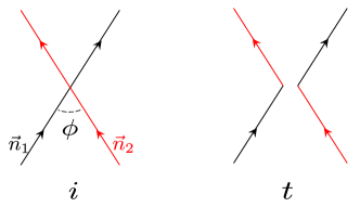
Refer to caption

(a)𝑎(a)

Refer to caption

(b)𝑏(b)

Figure 13: (a)𝑎(a) Intersecting lines (denoted by i𝑖i) and “touching” lines (denoted by t𝑡t). They are characterized by a geometrical angle ϕitalic-ϕ\phi and mix under the renormalization. In 𝒩=4𝒩4\mathcal{N}=4 SYM, we can consider the generalization of these lines which couple also to scalars. In that case, the black lines couple to n1Φsubscript𝑛1Φ\vec{n}_{1}\cdot\vec{\Phi} and the red lines couple to n2Φsubscript𝑛2Φ\vec{n}_{2}\cdot\vec{\Phi}. This introduces an additional angle cosθ=n1n2𝜃subscript𝑛1subscript𝑛2\cos\theta=\vec{n}_{1}\cdot\vec{n}_{2}. (b)𝑏(b) Two touching configurations (111 and 222) whose cross anomalous dimension will be computed in Appendix B.

4.1 Cross anomalous dimension in 𝒩=4𝒩4\mathcal{N}=4 SYM

Definition and the relation to amplitudes

The cross anomalous dimension matrix ΓcrosssubscriptΓcross\Gamma_{\rm cross} determines the renormalization group (RG) property of the Wilson lines with an intersection [28, 29]:

(μμ+β(g)g)𝒲AR+(Γcross)A𝒲BRB=0(A,B=i,t),\left(\mu\frac{\partial}{\partial\mu}+\beta(g)\frac{\partial}{\partial g}\right)\mathcal{W}^{\rm R}_{A}+\left(\Gamma_{\rm cross}\right)_{A}{}^{B}\mathcal{W}^{\rm R}_{B}=0\qquad(A,B=i,t)\,, (4.1)

Here μ𝜇\mu is the RG scale and 𝒲isubscript𝒲𝑖\mathcal{W}_{i} and 𝒲tsubscript𝒲𝑡\mathcal{W}_{t} denote the intersecting and the touching configurations respectively. The superscript R signifies the fact that the Wilson lines are renormalized and are related to the bare Wilson lines 𝒲Asubscript𝒲𝐴\mathcal{W}_{A} by the multiplicative renormalziation,

𝒲AR=(Z(μ,ϵ))A𝒲BB.superscriptsubscript𝒲𝐴Rsubscript𝑍𝜇italic-ϵ𝐴superscriptsubscript𝒲𝐵𝐵\mathcal{W}_{A}^{\rm R}=\left(Z(\mu,\epsilon)\right)_{A}{}^{B}\mathcal{W}_{B}\,. (4.2)

with ϵitalic-ϵ\epsilon being the UV cut-off. As we discuss in more detail later, in conformal field theories one can compute the cross anomalous dimension more directly from the expectation value of the bare Wilson lines by reading off the coefficient of logϵitalic-ϵ\log\epsilon, 𝒲eΓcrosslogϵsimilar-todelimited-⟨⟩𝒲superscript𝑒subscriptΓcrossitalic-ϵ\langle\mathcal{W}\rangle\sim e^{\Gamma_{\rm cross}\log\epsilon}.

The cross anomalous dimension is a function of the angle ϕitalic-ϕ\phi between the two intersecting lines. When the angle is analytically continued as ϕiφitalic-ϕ𝑖𝜑\phi\to i\varphi, it gives the so-called soft anomalous dimension. The soft anomalous dimension controls the IR divergence of the scattering amplitude of two massive quarks in the Regge kinematics, s,m2tΛQCD2much-greater-than𝑠superscript𝑚2𝑡much-greater-thansuperscriptsubscriptΛQCD2s,m^{2}\gg-t\gg\Lambda_{\rm QCD}^{2}, and describes how the soft gluons transfer the color degrees of freedom of the quarks. In that context, φ𝜑\varphi is the boost angle between the two quarks defined by

coshφ:=p1p2p12p22,assign𝜑subscript𝑝1subscript𝑝2superscriptsubscript𝑝12superscriptsubscript𝑝22\cosh\varphi:=-\frac{p_{1}\cdot p_{2}}{\sqrt{p_{1}^{2}p_{2}^{2}}}\,, (4.3)

with p1,2subscript𝑝12p_{1,2} being the four-momenta of the quarks. See [28, 29] for more details.

For the application to QCD, the limit φ𝜑\varphi\to\infty is of particular interest since it describes the high energy scattering of light partons. On the Wilson line side, this corresponds to an intersection of two light-like lines, see for instance [47, 48, 49]. The limit was studied also in 𝒩=4𝒩4\mathcal{N}=4 SYM: In [50], the self-crossing lightlike loop was analyzed up to nine loops. The analysis was pushed further in [51] in which the anomalous dimensions relevant for the limit were determined exactly in the large N𝑁N limit using the pentagon OPE decomposition [52]. In this paper, we focus on different limits, namely ϕφ0similar-toitalic-ϕ𝜑similar-to0\phi\sim\varphi\sim 0 and the near BPS limit, and compute the anomalous dimension exactly at finite N𝑁N.

Generalization in 𝒩=4𝒩4\mathcal{N}=4 SYM

In 𝒩=4𝒩4\mathcal{N}=4 SYM, one can consider a generalization of the cross anomalous dimension Γcross(ϕ,θ)subscriptΓcrossitalic-ϕ𝜃\Gamma_{\rm cross}(\phi,\theta) which depends on another angle θ𝜃\theta. To do so, we consider an intersection of the supersymmetric Wilson lines,

𝒲trPexp((iAμx˙μ+nΦ|x˙|)𝑑τ),similar-to𝒲trP𝑖subscript𝐴𝜇superscript˙𝑥𝜇𝑛Φ˙𝑥differential-d𝜏\mathcal{W}\sim{\rm tr}{\rm P}\exp\left(\int(iA_{\mu}\dot{x}^{\mu}+\vec{n}\cdot\vec{\Phi}|\dot{x}|)d\tau\right)\,, (4.4)

where the R-symmetry polarization n𝑛\vec{n} is a six-component unit vector which dictates the coupling to the scalars Φ=(Φ1,,Φ6)ΦsubscriptΦ1subscriptΦ6\vec{\Phi}=(\Phi_{1},\ldots,\Phi_{6}). The intersection of such lines can be characterized by the geometric angle ϕitalic-ϕ\phi and the R-symmetry angle θ𝜃\theta which is defined by

cosθ:=n1n2,assign𝜃subscript𝑛1subscript𝑛2\cos\theta:=\vec{n}_{1}\cdot\vec{n}_{2}\,, (4.5)

where n1,2subscript𝑛12\vec{n}_{1,2} are the R-symmetry polarizations of the two lines at the intersection point.

The supersymmetric Wilson line (4.4) naturally arises from the worldline action of the W𝑊W-boson in the Coulomb branch of 𝒩=4𝒩4\mathcal{N}=4 SYM. To be concrete, let us consider the symmetry breaking phase U(N+2)U(1)×U(1)×U(N)U𝑁2U1U1U𝑁{\rm U}(N+2)\to{\rm U}(1)\times{\rm U}(1)\times{\rm U}(N) dictated by the scalar expectation value

Φ=diag(m1n1,m2n2,0,,0N).delimited-⟨⟩Φdiagsubscript𝑚1subscript𝑛1subscript𝑚2subscript𝑛2subscript00𝑁\langle\vec{\Phi}\rangle={\rm diag}\left(m_{1}\vec{n}_{1}\,,m_{2}\vec{n}_{2},\underbrace{0,\ldots,0}_{N}\right)\,. (4.6)

In this phase, we have two kinds of W𝑊W-bosons, one coming from the (1,k)1𝑘(1,k) (or (k,1)𝑘1(k,1)) component and the other coming from the (2,k)2𝑘(2,k) (or (k,2)𝑘2(k,2)) component of the gauge field. In the limit m1,21much-greater-thansubscript𝑚121m_{1,2}\gg 1, they can be treated as classical probe particles and their coupling to the unbroken U(N)𝑁(N) degrees of freedom is given precisely by (4.4). Thus Γcross(ϕ,θ)subscriptΓcrossitalic-ϕ𝜃\Gamma_{\rm cross}(\phi,\theta) gives a natural generalization of the cross anomalous dimension in QCD and it characterizes the IR divergence of the scattering of massive W𝑊W-bosons after the analytic continuation ϕiφitalic-ϕ𝑖𝜑\phi\to i\varphi.

When ϕ=θitalic-ϕ𝜃\phi=\theta, the whole configuration becomes BPS and the anomalous dimension Γcross(ϕ,θ)subscriptΓcrossitalic-ϕ𝜃\Gamma_{\rm cross}(\phi,\theta) vanishes. Expanding Γcross(ϕ,θ)subscriptΓcrossitalic-ϕ𝜃\Gamma_{\rm cross}(\phi,\theta) around this limit, we obtain161616The relation between ΓcrosssubscriptΓcross\Gamma_{\rm cross} and γ^crosssubscript^𝛾cross\hat{\gamma}_{\rm cross} parallels the relation between the cusp anomalous dimension and the Bremsstralung function [25].

Γcross(ϕ,θ)=(ϕθ)γcross(θ)+O((ϕθ)2).subscriptΓcrossitalic-ϕ𝜃italic-ϕ𝜃subscript𝛾cross𝜃𝑂superscriptitalic-ϕ𝜃2\Gamma_{\rm cross}(\phi,\theta)=(\phi-\theta)\gamma_{\rm cross}(\theta)+O((\phi-\theta)^{2})\,. (4.7)

In what follows, we compute the first coefficient γcross(θ)subscript𝛾cross𝜃\gamma_{\rm cross}(\theta) exactly as a function of λ𝜆\lambda and N𝑁N.

4.2 Two-point function of intersections

Let us explain in more detail how to extract the cross anomalous dimension from the expectation values of the bare Wilson lines. The key idea is to regard them as the two-point functions of intersections.

To be concrete, consider the intersection of the following two Wilson lines on R4superscript𝑅4R^{4},

𝒲1,2=Pexp𝑑τ(iAx˙1,2+Φn1,2|x˙1,2|),subscript𝒲12Psubscriptsuperscriptdifferential-d𝜏𝑖𝐴subscript˙𝑥12Φsubscript𝑛12subscript˙𝑥12\mathcal{W}_{1,2}={\rm P}\exp\int^{\infty}_{-\infty}d\tau\left(iA\cdot\dot{x}_{1,2}+\vec{\Phi}\cdot\vec{n}_{1,2}|\dot{x}_{1,2}|\right)\,, (4.8)

with

x˙1=(1,0,0,0),subscript˙𝑥11000\displaystyle\dot{x}_{1}=(1,0,0,0)\,,\qquad x˙2=(cosϕ,sinϕ,0,0),subscript˙𝑥2italic-ϕitalic-ϕ00\displaystyle\dot{x}_{2}=(\cos\phi,\sin\phi,0,0)\,, (4.9)
n1=(1,0,0,0,0,0),subscript𝑛1100000\displaystyle n_{1}=(1,0,0,0,0,0)\,,\qquad n2=(cosθ,sinθ,0,0,0,0).subscript𝑛2𝜃𝜃0000\displaystyle n_{2}=(\cos\theta,\sin\theta,0,0,0,0)\,.

In addition to the obvious intersection at the origin, the lines intersect also at infinity. This is easier to see if one maps the configuration to S2superscript𝑆2S^{2} using the conformal transformation

X1=2x11+x12+x22,X2=2x11+x12+x22,X3=1x12x221+x12+x22.formulae-sequencesubscript𝑋12subscript𝑥11superscriptsubscript𝑥12superscriptsubscript𝑥22formulae-sequencesubscript𝑋22subscript𝑥11superscriptsubscript𝑥12superscriptsubscript𝑥22subscript𝑋31superscriptsubscript𝑥12superscriptsubscript𝑥221superscriptsubscript𝑥12superscriptsubscript𝑥22X_{1}=\frac{2x_{1}}{1+x_{1}^{2}+x_{2}^{2}}\,,\quad X_{2}=\frac{-2x_{1}}{1+x_{1}^{2}+x_{2}^{2}}\,,\quad X_{3}=\frac{1-x_{1}^{2}-x_{2}^{2}}{1+x_{1}^{2}+x_{2}^{2}}\,. (4.10)

Here X𝑋X’s are the embedding coordinates of S2superscript𝑆2S^{2} while x𝑥x’s are the coordinates on R2superscript𝑅2R^{2} inside R4superscript𝑅4R^{4}. The two intersections are mapped to the north and the south poles of S2superscript𝑆2S^{2}, see figure 14.

Refer to caption
Figure 14: Intersecting lines mapped onto S2superscript𝑆2S^{2}. The black and the red lines denote 𝒲1subscript𝒲1\mathcal{W}_{1} and 𝒲2subscript𝒲2\mathcal{W}_{2} respectively. On S2superscript𝑆2S^{2}, the configuration contains two intersections, one at the north pole and the other at the south pole. At each intersection (denoted by white circles), one can make either of the two choices, i𝑖i and t𝑡t. This leads to the 2×2222\times 2 matrix structure of the cross anomalous dimension.

To extract the cross anomalous dimension, one has to consider the operator mixing: For each intersection, we can either let the lines intersect (to be denoted by i𝑖i) or resolve the intersection and make the lines touching (to be denoted by t𝑡t). Since there are two intersections, we have in total four different configurations of the Wilson lines which we denote by 𝒲iisubscript𝒲𝑖𝑖\mathcal{W}_{ii}, 𝒲itsubscript𝒲𝑖𝑡\mathcal{W}_{it}, 𝒲tisubscript𝒲𝑡𝑖\mathcal{W}_{ti} and 𝒲ttsubscript𝒲𝑡𝑡\mathcal{W}_{tt}. They can be regarded as two-point functions of “operators”, labeled by i𝑖i and t𝑡t, sitting at the intersections.

These four choices of two-point functions can be naturally organized into a 2×2222\times 2 matrix

𝕎:=(𝒲ii𝒲it𝒲ti𝒲tt)=(i|exp(DlogϵUVrIR)|ii|exp(DlogϵUVrIR)|tt|exp(DlogϵUVrIR)|it|exp(DlogϵUVrIR)|t).assign𝕎delimited-⟨⟩subscript𝒲𝑖𝑖delimited-⟨⟩subscript𝒲𝑖𝑡delimited-⟨⟩subscript𝒲𝑡𝑖delimited-⟨⟩subscript𝒲𝑡𝑡quantum-operator-product𝑖𝐷subscriptitalic-ϵUVsubscript𝑟IR𝑖quantum-operator-product𝑖𝐷subscriptitalic-ϵUVsubscript𝑟IR𝑡quantum-operator-product𝑡𝐷subscriptitalic-ϵUVsubscript𝑟IR𝑖quantum-operator-product𝑡𝐷subscriptitalic-ϵUVsubscript𝑟IR𝑡\mathbb{W}:=\left(\begin{array}[]{cc}\langle\mathcal{W}_{ii}\rangle&\langle\mathcal{W}_{it}\rangle\\ \langle\mathcal{W}_{ti}\rangle&\langle\mathcal{W}_{tt}\rangle\end{array}\right)=\left(\begin{array}[]{cc}\langle i|\exp\left(D\log\frac{\epsilon_{\rm UV}}{r_{\rm IR}}\right)|i\rangle&\langle i|\exp\left(D\log\frac{\epsilon_{\rm UV}}{r_{\rm IR}}\right)|t\rangle\\ \langle t|\exp\left(D\log\frac{\epsilon_{\rm UV}}{r_{\rm IR}}\right)|i\rangle&\langle t|\exp\left(D\log\frac{\epsilon_{\rm UV}}{r_{\rm IR}}\right)|t\rangle\end{array}\right)\,. (4.11)

Here i,t|bra𝑖𝑡\langle i,t| and |i,tket𝑖𝑡|i,t\rangle denote the intersections at the origin and infinity respectively and D𝐷D is the dilatation operator. ϵUVsubscriptitalic-ϵUV\epsilon_{\rm UV} and rIRsubscript𝑟IRr_{\rm IR} are the UV and the IR cutoffs. 𝕎𝕎\mathbb{W} can be expressed alternatively in terms of the cross anomalous dimension ΓcrosssubscriptΓcross\Gamma_{\rm cross} and the overlap η𝜂\eta as

𝕎=eΓcrosslog(ϵUV/rIR)η,𝕎superscript𝑒subscriptΓcrosssubscriptitalic-ϵUVsubscript𝑟IR𝜂\mathbb{W}=e^{\Gamma_{\rm cross}\log(\epsilon_{\rm UV}/r_{\rm IR})}\cdot\eta\,, (4.12)

where ΓcrosssubscriptΓcross\Gamma_{\rm cross} and η𝜂\eta are 2×2222\times 2 matrices defined by

(i|,t|)Γcross:=(i|D,t|D),η:=(i|ii|tt|it|t).formulae-sequenceassignbra𝑖bra𝑡subscriptΓcrossbra𝑖𝐷bra𝑡𝐷assign𝜂inner-product𝑖𝑖inner-product𝑖𝑡inner-product𝑡𝑖inner-product𝑡𝑡\displaystyle\left(\begin{array}[]{cc}\langle i|\,,&\langle t|\end{array}\right)\Gamma_{\rm cross}:=\left(\begin{array}[]{cc}\langle i|D\,,&\langle t|D\end{array}\right)\,,\qquad\quad\eta:=\left(\begin{array}[]{cc}\langle i|i\rangle&\langle i|t\rangle\\ \langle t|i\rangle&\langle t|t\rangle\end{array}\right)\,. (4.13)

In the near BPS limit θϕsimilar-to𝜃italic-ϕ\theta\sim\phi, both η𝜂\eta and ΓcrosssubscriptΓcross\Gamma_{\rm cross} can be expanded in powers of (ϕθ)italic-ϕ𝜃(\phi-\theta),

η=η0+(ϕθ)η1+,Γcross=(ϕθ)γcross+.formulae-sequence𝜂subscript𝜂0italic-ϕ𝜃subscript𝜂1subscriptΓcrossitalic-ϕ𝜃subscript𝛾cross\eta=\eta_{0}+(\phi-\theta)\eta_{1}+\cdots\,,\qquad\Gamma_{\rm cross}=(\phi-\theta)\gamma_{\rm cross}+\cdots\,. (4.14)

We then obtain the following expansion of the two-point function matrix 𝕎𝕎\mathbb{W}:

𝕎=𝕎0+(ϕθ)𝕎1+,𝕎subscript𝕎0italic-ϕ𝜃subscript𝕎1\displaystyle\mathbb{W}=\mathbb{W}_{0}+(\phi-\theta)\mathbb{W}_{1}+\cdots\,, (4.15)
𝕎0=η0,𝕎1=η1+(γcrossη0)log(ϵUV/rIR).formulae-sequencesubscript𝕎0subscript𝜂0subscript𝕎1subscript𝜂1subscript𝛾crosssubscript𝜂0subscriptitalic-ϵUVsubscript𝑟IR\displaystyle\mathbb{W}_{0}=\eta_{0}\,,\qquad\mathbb{W}_{1}=\eta_{1}+(\gamma_{\rm cross}\cdot\eta_{0})\log(\epsilon_{\rm UV}/r_{\rm IR})\,.

Thus γcrosssubscript𝛾cross\gamma_{\rm cross} is given by the coefficient of the logarithm in 𝕎1subscript𝕎1\mathbb{W}_{1}, multiplied by (𝕎0)1superscriptsubscript𝕎01(\mathbb{W}_{0})^{-1},

γcross=(𝕎1|logϵUVrIR)(𝕎0)1,subscript𝛾crossevaluated-atsubscript𝕎1subscriptitalic-ϵUVsubscript𝑟IRsuperscriptsubscript𝕎01\gamma_{\rm cross}=\left(\left.\mathbb{W}_{1}\right|_{\log\frac{\epsilon_{\rm UV}}{r_{\rm IR}}}\right)\cdot(\mathbb{W}_{0})^{-1}\,, (4.16)

where 𝕎0subscript𝕎0\mathbb{W}_{0} is nothing but the expectation value in the BPS limit:

𝕎0(θ)=(𝒲ii𝒲it𝒲ti𝒲tt)|ϕ=θ.subscript𝕎0𝜃evaluated-atdelimited-⟨⟩subscript𝒲𝑖𝑖delimited-⟨⟩subscript𝒲𝑖𝑡delimited-⟨⟩subscript𝒲𝑡𝑖delimited-⟨⟩subscript𝒲𝑡𝑡italic-ϕ𝜃\mathbb{W}_{0}(\theta)=\left.\left(\begin{array}[]{cc}\langle\mathcal{W}_{ii}\rangle&\langle\mathcal{W}_{it}\rangle\\ \langle\mathcal{W}_{ti}\rangle&\langle\mathcal{W}_{tt}\rangle\end{array}\right)\right|_{\phi=\theta}\,. (4.17)

4.3 Cross anomalous dimension from localization

We now relate γcrosssubscript𝛾cross\gamma_{\rm cross} given in (4.16) to the localization computation. This can be done by following the arguments in [25, 23, 26], which we briefly review below171717See section 4.2 of [26] for more detailed explanation..

The first step is to start with the BPS limit θ=ϕ𝜃italic-ϕ\theta=\phi of (4.8) and deform θ𝜃\theta slightly. This amounts to inserting a scalar on the second Wilson line

δ𝒲2=δθ×𝑑τP[Φ(τ)𝒲2],𝛿subscript𝒲2𝛿𝜃superscriptsubscriptdifferential-d𝜏Pdelimited-[]superscriptΦ𝜏subscript𝒲2\delta\mathcal{W}_{2}=\delta\theta\times\int_{-\infty}^{\infty}d\tau\,{\rm P}\left[\Phi^{\prime}(\tau)\mathcal{W}_{2}\right]\,, (4.18)

with

Φ(τ)=sinθΦ1+cosθΦ2|xμ=(τcosθ,τsinθ,0,0,0,0).superscriptΦ𝜏𝜃subscriptΦ1evaluated-at𝜃subscriptΦ2superscript𝑥𝜇𝜏𝜃𝜏𝜃0000\Phi^{\prime}(\tau)=\left.-\sin\theta\Phi_{1}+\cos\theta\Phi_{2}\right|_{x^{\mu}=(\tau\cos\theta,\tau\sin\theta,0,0,0,0)}\,. (4.19)

Now, using the invariance under the dilatation around the origin, we can determine the position dependence of the scalar insertion as

Φ(τ)=1|τ|Φ(τ=1),delimited-⟨⟩superscriptΦ𝜏1𝜏delimited-⟨⟩superscriptΦ𝜏1\langle\Phi^{\prime}(\tau)\cdots\rangle=\frac{1}{|\tau|}\langle\Phi^{\prime}(\tau=1)\cdots\rangle\,, (4.20)

where we denoted all the other parts (the Wilson lines 𝒲1,2subscript𝒲12\mathcal{W}_{1,2} and possible resolutions of the intersections etc.) by \cdots. From this, one can see that the integral of τ𝜏\tau produces the logarithmic divergence and its coefficient is given by the expectation value of the Wilson loops with the ΦsuperscriptΦ\Phi^{\prime} insertion. More explicitly, we have the relation

𝕎1|logϵUVrIR=2(𝒲ii𝒲it𝒲ti𝒲tt)|ϕ=θ,evaluated-atsubscript𝕎1subscriptitalic-ϵUVsubscript𝑟IRevaluated-at2delimited-⟨⟩subscriptsuperscript𝒲𝑖𝑖delimited-⟨⟩subscriptsuperscript𝒲𝑖𝑡delimited-⟨⟩subscriptsuperscript𝒲𝑡𝑖delimited-⟨⟩subscriptsuperscript𝒲𝑡𝑡italic-ϕ𝜃\displaystyle\left.\mathbb{W}_{1}\right|_{\log\frac{\epsilon_{\rm UV}}{r_{\rm IR}}}=2\left.\left(\begin{array}[]{cc}\langle\mathcal{W}^{\prime}_{ii}\rangle&\langle\mathcal{W}^{\prime}_{it}\rangle\\ \langle\mathcal{W}^{\prime}_{ti}\rangle&\langle\mathcal{W}^{\prime}_{tt}\rangle\end{array}\right)\right|_{\phi=\theta}\,, (4.21)

where 𝒲ABsubscriptsuperscript𝒲𝐴𝐵\mathcal{W}^{\prime}_{AB} is the Wilson line 𝒲ABsubscript𝒲𝐴𝐵\mathcal{W}_{AB} with ΦsuperscriptΦ\Phi^{\prime} inserted at (cosθ,sinθ,0,0,0,0)𝜃𝜃0000(\cos\theta,\sin\theta,0,0,0,0). The factor of 222 comes from summing up contributions from 0𝑑τsubscriptsuperscript0differential-d𝜏\int^{\infty}_{0}d\tau and 0𝑑τsubscriptsuperscript0differential-d𝜏\int^{0}_{-\infty}d\tau.

The second step is to map the whole configuration to S2superscript𝑆2S^{2} using (4.10). We then get two great circles whose contour are given by

(x1,x2,x3)={(0,sint,cost)(𝒲1)(sinθsint,cosθsint,cost)(𝒲2),subscript𝑥1subscript𝑥2subscript𝑥3cases0𝑡𝑡subscript𝒲1𝜃𝑡𝜃𝑡𝑡subscript𝒲2(x_{1},x_{2},x_{3})=\begin{cases}(0,\sin t,-\cos t)\qquad&(\mathcal{W}_{1})\\ (-\sin\theta\sin t,\cos\theta\sin t,-\cos t)\qquad&(\mathcal{W}_{2})\end{cases}\,, (4.22)

with t(π,π)𝑡𝜋𝜋t\in(-\pi,\pi). They couple to Φ1superscriptΦ1\Phi^{1} and cosθΦ1+sinθΦ2𝜃superscriptΦ1𝜃superscriptΦ2\cos\theta\Phi^{1}+\sin\theta\Phi^{2} respectively and satisfy the 1/8181/8 BPS condition (2.1). Under this map, the insertion Φ(τ=1)superscriptΦ𝜏1\Phi^{\prime}(\tau=1) is mapped to the insertion at a point tesubscript𝑡𝑒t_{e} where 𝒲2subscript𝒲2\mathcal{W}_{2} intersects with the equator of S2superscript𝑆2S^{2} (see figure 14).

The third step is to replace ΦsuperscriptΦ\Phi^{\prime} at tesubscript𝑡𝑒t_{e} with ΦiΦ4=:Φ~\Phi^{\prime}-i\Phi_{4}=:-\tilde{\Phi}. This replacement does not affect the expectation values since the correlator with Φ4subscriptΦ4\Phi_{4} vanishes owing to the charge conservation. We then use the fact that the insertion of Φ~~Φ\tilde{\Phi} corresponds to the insertion of the field strength in 2d YM [11, 16]. Therefore its expectation value can be computed by taking the area derivative. In our setup there are two regions with area 2(πθ)2𝜋𝜃2(\pi-\theta), and changing θ𝜃\theta by δθ𝛿𝜃\delta\theta leads to a total change (decrease) of the area by 4δθ4𝛿𝜃4\delta\theta. We thus have the relation

(𝒲ii𝒲it𝒲ti𝒲tt)|ϕ=θ=14θ𝕎0(θ),evaluated-atdelimited-⟨⟩subscriptsuperscript𝒲𝑖𝑖delimited-⟨⟩subscriptsuperscript𝒲𝑖𝑡delimited-⟨⟩subscriptsuperscript𝒲𝑡𝑖delimited-⟨⟩subscriptsuperscript𝒲𝑡𝑡italic-ϕ𝜃14subscript𝜃subscript𝕎0𝜃\left.\left(\begin{array}[]{cc}\langle\mathcal{W}^{\prime}_{ii}\rangle&\langle\mathcal{W}^{\prime}_{it}\rangle\\ \langle\mathcal{W}^{\prime}_{ti}\rangle&\langle\mathcal{W}^{\prime}_{tt}\rangle\end{array}\right)\right|_{\phi=\theta}=\frac{1}{4}\partial_{\theta}\mathbb{W}_{0}(\theta)\,, (4.23)

with 𝕎0subscript𝕎0\mathbb{W}_{0} is the expectation value in the BPS limit (4.17). Combined with (4.21), it gives

𝕎1|logϵUVrIR=12θ𝕎0(θ).evaluated-atsubscript𝕎1subscriptitalic-ϵUVsubscript𝑟IR12subscript𝜃subscript𝕎0𝜃\left.\mathbb{W}_{1}\right|_{\log\frac{\epsilon_{\rm UV}}{r_{\rm IR}}}=\frac{1}{2}\partial_{\theta}\mathbb{W}_{0}(\theta)\,. (4.24)

Using (4.16), we get the formula relating γcrosssubscript𝛾cross\gamma_{\rm cross} to the BPS Wilson loops

γcross=12(θ𝕎0)(𝕎0)1.subscript𝛾cross12subscript𝜃subscript𝕎0superscriptsubscript𝕎01\gamma_{\rm cross}=\frac{1}{2}\left(\partial_{\theta}\mathbb{W}_{0}\right)\cdot\left(\mathbb{W}_{0}\right)^{-1}\,. (4.25)

Before we proceed, let us comment on the normalization. In what follows, we normalize 𝕎0subscript𝕎0\mathbb{W}_{0} by dividing the path-ordered exponentials by a common factor N2superscript𝑁2N^{2}. This is a natural normalization for discussing the renormalization of open intersecting lines (see [27, 28, 29]) and makes ΓcrosssubscriptΓcross\Gamma_{\rm cross} more symmetric. However it does not coincide with the normalization used in some of the literature in which they discuss the renormalization of closed loops. We will later translate the final result to such a normalization.

The last step is to compute 𝕎0subscript𝕎0\mathbb{W}_{0}. Let us first consider 𝒲ttdelimited-⟨⟩subscript𝒲𝑡𝑡\langle\mathcal{W}_{tt}\rangle. Since both intersections are resolved, it coincides with a correlator of two disconnected loops. Thus, setting A1=2(π+θ)subscript𝐴12𝜋𝜃A_{1}=2(\pi+\theta) and A2=2(πθ)subscript𝐴22𝜋𝜃A_{2}=2(\pi-\theta) in (2.46), we get

𝒲tt|ϕ=θ=𝒞1𝒞2du18π2g2du28π2g2Δ¯(u1,u2)f2(π+θ)(u1)f2(πθ)(u2)M.evaluated-atdelimited-⟨⟩subscript𝒲𝑡𝑡italic-ϕ𝜃subscriptdelimited-⟨⟩subscriptcontour-integralprecedessubscript𝒞1subscript𝒞2𝑑subscript𝑢18superscript𝜋2superscript𝑔2𝑑subscript𝑢28superscript𝜋2superscript𝑔2¯Δsubscript𝑢1subscript𝑢2subscript𝑓2𝜋𝜃subscript𝑢1subscript𝑓2𝜋𝜃subscript𝑢2𝑀\left.\langle\mathcal{W}_{tt}\rangle\right|_{\phi=\theta}=\left<\oint_{\mathcal{C}_{1}\prec\mathcal{C}_{2}}\frac{du_{1}}{8\pi^{2}g^{2}}\frac{du_{2}}{8\pi^{2}g^{2}}\bar{\Delta}(u_{1},u_{2})f_{2(\pi+\theta)}(u_{1})f_{2(\pi-\theta)}(u_{2})\right>_{M}\,. (4.26)

Using the result in the literature, we can compute its large N𝑁N limit as181818The result (4.27) can be obtained from (3.57) by setting A1A3=2(π+θ)subscript𝐴1subscript𝐴32𝜋𝜃A_{1}-A_{3}=2(\pi+\theta) and A2=2(πθ)subscript𝐴22𝜋𝜃A_{2}=2(\pi-\theta).

𝒲tt|ϕ=θ=N(1θ2πgθ)2+πgθ1θ2θ3N2+1N2k=1k(kθ)2(ρθ)2k.evaluated-atdelimited-⟨⟩subscript𝒲𝑡𝑡italic-ϕ𝜃𝑁superscriptsuperscriptsubscript1𝜃2𝜋subscript𝑔𝜃2𝜋subscript𝑔𝜃superscriptsubscript1𝜃superscriptsubscript2𝜃3superscript𝑁21superscript𝑁2superscriptsubscript𝑘1𝑘superscriptsuperscriptsubscript𝑘𝜃2superscriptsubscript𝜌𝜃2𝑘\left.\langle\mathcal{W}_{tt}\rangle\right|_{\phi=\theta}\overset{N\to\infty}{=}\left(\frac{\mathcal{I}_{1}^{\theta}}{2\pi g_{\theta}}\right)^{2}+\frac{\pi g_{\theta}\mathcal{I}_{1}^{\theta}\mathcal{I}_{2}^{\theta}}{3N^{2}}+\frac{1}{N^{2}}\sum_{k=1}^{\infty}\frac{k(\mathcal{I}_{k}^{\theta})^{2}}{(\rho_{\theta})^{2k}}\,. (4.27)

Second, 𝒲ti(=𝒲it)annotateddelimited-⟨⟩subscript𝒲𝑡𝑖absentdelimited-⟨⟩subscript𝒲𝑖𝑡\langle\mathcal{W}_{ti}\rangle(=\langle\mathcal{W}_{it}\rangle) is a single-intersection loop with areas A1=2(π+θ)subscript𝐴12𝜋𝜃A_{1}=2(\pi+\theta) and A2=2(πθ)subscript𝐴22𝜋𝜃A_{2}=2(\pi-\theta) (or equivalently, a figure-eight loop with areas A¯1=A¯2=2(πθ)subscript¯𝐴1subscript¯𝐴22𝜋𝜃\bar{A}_{1}=\bar{A}_{2}=2(\pi-\theta)). We thus get from (3.31)

𝒲ti|ϕ=θ=4πg2iN𝒞1𝒞2du18π2g2du28π2g2Δ¯(u1,u2)f2(π+θ)(u1)f2(πθ)(u2)u1u2M.evaluated-atdelimited-⟨⟩subscript𝒲𝑡𝑖italic-ϕ𝜃4𝜋superscript𝑔2𝑖𝑁subscriptdelimited-⟨⟩subscriptcontour-integralprecedessubscript𝒞1subscript𝒞2𝑑subscript𝑢18superscript𝜋2superscript𝑔2𝑑subscript𝑢28superscript𝜋2superscript𝑔2¯Δsubscript𝑢1subscript𝑢2subscript𝑓2𝜋𝜃subscript𝑢1subscript𝑓2𝜋𝜃subscript𝑢2subscript𝑢1subscript𝑢2𝑀\left.\langle\mathcal{W}_{ti}\rangle\right|_{\phi=\theta}=\frac{4\pi g^{2}i}{N}\left<\oint_{\mathcal{C}_{1}\prec\mathcal{C}_{2}}\frac{du_{1}}{8\pi^{2}g^{2}}\frac{du_{2}}{8\pi^{2}g^{2}}\bar{\Delta}(u_{1},u_{2})\frac{f_{2(\pi+\theta)}(u_{1})f_{2(\pi-\theta)}(u_{2})}{u_{1}-u_{2}}\right>_{M}\,. (4.28)

Here the extra factor 1/N1𝑁1/N comes from the normalization that we adopted. The large N𝑁N limit can be computed from (3.42) as

𝒲ti|ϕ=θ=N12πN(0θ1θgθ+k=1kθk+1θg(ρθ2k1+(1)kρθρθ12)).evaluated-atdelimited-⟨⟩subscript𝒲𝑡𝑖italic-ϕ𝜃𝑁12𝜋𝑁superscriptsubscript0𝜃superscriptsubscript1𝜃subscript𝑔𝜃superscriptsubscript𝑘1superscriptsubscript𝑘𝜃superscriptsubscript𝑘1𝜃𝑔superscriptsubscript𝜌𝜃2𝑘1superscript1𝑘subscript𝜌𝜃superscriptsubscript𝜌𝜃12\displaystyle\left.\langle\mathcal{W}_{ti}\rangle\right|_{\phi=\theta}\overset{N\to\infty}{=}\frac{1}{2\pi N}\left(\frac{\mathcal{I}_{0}^{\theta}\mathcal{I}_{1}^{\theta}}{g_{\theta}}+\sum_{k=1}^{\infty}\frac{\mathcal{I}_{k}^{\theta}\mathcal{I}_{k+1}^{\theta}}{g}\left(\rho_{\theta}^{-2k-1}+(-1)^{k}\frac{\rho_{\theta}-\rho_{\theta}^{-1}}{2}\right)\right)\,. (4.29)

Finally, 𝒲iidelimited-⟨⟩subscript𝒲𝑖𝑖\langle\mathcal{W}_{ii}\rangle is a two-intersection loop which we computed in (3.56). Setting A1=2(π+θ)subscript𝐴12𝜋𝜃A_{1}=2(\pi+\theta), A2=2πsubscript𝐴22𝜋A_{2}=2\pi and A3=2θsubscript𝐴32𝜃A_{3}=2\theta, we get

𝒲ii|ϕ=θ=𝒞1𝒞2du18π2g2du28π2g2Δ¯f2π(u1)f2π(u2)Mevaluated-atdelimited-⟨⟩subscript𝒲𝑖𝑖italic-ϕ𝜃subscriptdelimited-⟨⟩subscriptcontour-integralprecedessubscript𝒞1subscript𝒞2𝑑subscript𝑢18superscript𝜋2superscript𝑔2𝑑subscript𝑢28superscript𝜋2superscript𝑔2¯Δsubscript𝑓2𝜋subscript𝑢1subscript𝑓2𝜋subscript𝑢2𝑀\displaystyle\left.\langle\mathcal{W}_{ii}\rangle\right|_{\phi=\theta}=\left<\oint_{\mathcal{C}_{1}\prec\mathcal{C}_{2}}\frac{du_{1}}{8\pi^{2}g^{2}}\frac{du_{2}}{8\pi^{2}g^{2}}\bar{\Delta}f_{2\pi}(u_{1})f_{2\pi}(u_{2})\right>_{M} (4.30)
+(4πg2)2N2𝒞1𝒞2du18π2g2du28π2g2Δ¯f2π(u1)f2π(u2)f2(π+θ)(u1)f2(πθ)(u2)(u1u2)2M.superscript4𝜋superscript𝑔22superscript𝑁2subscriptdelimited-⟨⟩subscriptcontour-integralprecedessubscript𝒞1subscript𝒞2𝑑subscript𝑢18superscript𝜋2superscript𝑔2𝑑subscript𝑢28superscript𝜋2superscript𝑔2¯Δsubscript𝑓2𝜋subscript𝑢1subscript𝑓2𝜋subscript𝑢2subscript𝑓2𝜋𝜃subscript𝑢1subscript𝑓2𝜋𝜃subscript𝑢2superscriptsubscript𝑢1subscript𝑢22𝑀\displaystyle+\frac{(4\pi g^{2})^{2}}{N^{2}}\left<\oint_{\mathcal{C}_{1}\prec\mathcal{C}_{2}}\frac{du_{1}}{8\pi^{2}g^{2}}\frac{du_{2}}{8\pi^{2}g^{2}}\bar{\Delta}\frac{f_{2\pi}(u_{1})f_{2\pi}(u_{2})-f_{2(\pi+\theta)}(u_{1})f_{2(\pi-\theta)}(u_{2})}{(u_{1}-u_{2})^{2}}\right>_{M}\,.

The large N𝑁N limit can be computed from (LABEL:eq:largeNdoubleinter), and the result reads

𝒲ii|ϕ=θ=N(102πg)2+gπ10203N2+k=1k[(ρθ2k(1)k)(kθ)2+(1)k(k0)2]N2.evaluated-atdelimited-⟨⟩subscript𝒲𝑖𝑖italic-ϕ𝜃𝑁superscriptsuperscriptsubscript102𝜋𝑔2𝑔𝜋superscriptsubscript10superscriptsubscript203superscript𝑁2superscriptsubscript𝑘1𝑘delimited-[]superscriptsubscript𝜌𝜃2𝑘superscript1𝑘superscriptsuperscriptsubscript𝑘𝜃2superscript1𝑘superscriptsuperscriptsubscript𝑘02superscript𝑁2\displaystyle\left.\langle\mathcal{W}_{ii}\rangle\right|_{\phi=\theta}\overset{N\to\infty}{=}\left(\frac{\mathcal{I}_{1}^{0}}{2\pi g}\right)^{2}+\frac{g\pi\mathcal{I}_{1}^{0}\mathcal{I}_{2}^{0}}{3N^{2}}+\sum_{k=1}^{\infty}\frac{k\left[\left(\rho_{\theta}^{-2k}-(-1)^{k}\right)(\mathcal{I}_{k}^{\theta})^{2}+(-1)^{k}(\mathcal{I}_{k}^{0})^{2}\right]}{N^{2}}\,. (4.31)

Note that these expectation values satisfy the following relation (at finite N𝑁N)

θ𝒲ii|ϕ=θ=8πg2N𝒲ti|ϕ=θ,θ𝒲ti|ϕ=θ=8πg2N𝒲tt|ϕ=θ.formulae-sequenceevaluated-atsubscript𝜃delimited-⟨⟩subscript𝒲𝑖𝑖italic-ϕ𝜃evaluated-at8𝜋superscript𝑔2𝑁delimited-⟨⟩subscript𝒲𝑡𝑖italic-ϕ𝜃evaluated-atsubscript𝜃delimited-⟨⟩subscript𝒲𝑡𝑖italic-ϕ𝜃evaluated-at8𝜋superscript𝑔2𝑁delimited-⟨⟩subscript𝒲𝑡𝑡italic-ϕ𝜃\partial_{\theta}\left.\langle\mathcal{W}_{ii}\rangle\right|_{\phi=\theta}=-\frac{8\pi g^{2}}{N}\left.\langle\mathcal{W}_{ti}\rangle\right|_{\phi=\theta}\,,\qquad\partial_{\theta}\left.\langle\mathcal{W}_{ti}\rangle\right|_{\phi=\theta}=-\frac{8\pi g^{2}}{N}\left.\langle\mathcal{W}_{tt}\rangle\right|_{\phi=\theta}\,. (4.32)

They are simply the loop equations written in terms of θ𝜃\theta-derivatives, but one can also verify them directly from (4.26), (4.28) and (4.30).

These expressions, together with the relation (4.25), give the exact cross anomalous dimension in the near BPS limit of the U(N)𝑁(N) theory. Using the relations (4.32), we get

γcrosssubscript𝛾cross\displaystyle\gamma_{\rm cross} =1det𝕎0(04πg2Ndet𝕎0𝒲tiθ𝒲tt24πg2𝒲tt2N𝒲iiθ𝒲tt2+4πg2𝒲ti𝒲ttN)|ϕ=θ.absentevaluated-at1subscript𝕎004𝜋superscript𝑔2𝑁subscript𝕎0delimited-⟨⟩subscript𝒲𝑡𝑖subscript𝜃delimited-⟨⟩subscript𝒲𝑡𝑡24𝜋superscript𝑔2superscriptdelimited-⟨⟩subscript𝒲𝑡𝑡2𝑁delimited-⟨⟩subscript𝒲𝑖𝑖subscript𝜃delimited-⟨⟩subscript𝒲𝑡𝑡24𝜋superscript𝑔2delimited-⟨⟩subscript𝒲𝑡𝑖delimited-⟨⟩subscript𝒲𝑡𝑡𝑁italic-ϕ𝜃\displaystyle=\left.\frac{1}{\det\mathbb{W}_{0}}\left(\begin{array}[]{cc}0&-\frac{4\pi g^{2}}{N}\det\mathbb{W}_{0}\\ -\frac{\langle\mathcal{W}_{ti}\rangle\partial_{\theta}\langle\mathcal{W}_{tt}\rangle}{2}-\frac{4\pi g^{2}\langle\mathcal{W}_{tt}\rangle^{2}}{N}&\frac{\langle\mathcal{W}_{ii}\rangle\partial_{\theta}\langle\mathcal{W}_{tt}\rangle}{2}+\frac{4\pi g^{2}\langle\mathcal{W}_{ti}\rangle\langle\mathcal{W}_{tt}\rangle}{N}\end{array}\right)\right|_{\phi=\theta}\,. (4.33)

Note in particular that the entries in the first row are 00 and 4πg2/N4𝜋superscript𝑔2𝑁-4\pi g^{2}/N at all orders in λ𝜆\lambda and N𝑁N. Epanding the result at large N𝑁N, we get

γcrosssubscript𝛾cross\displaystyle\gamma_{\rm cross} =N(04πg2N4πg2h1+h0h2Nh0+4πg2h2+h0(h2)2h1h0h3+h4N2),𝑁04𝜋superscript𝑔2𝑁4𝜋superscript𝑔2subscript1subscript0subscript2𝑁subscript04𝜋superscript𝑔2subscript2subscript0superscriptsubscript22subscript1subscript0subscript3subscript4superscript𝑁2\displaystyle\overset{N\to\infty}{=}\left(\begin{array}[]{cc}0&-\frac{4\pi g^{2}}{N}\\ -\frac{4\pi g^{2}h_{1}+h_{0}h_{2}}{N}&h_{0}+\frac{4\pi g^{2}h_{2}+\frac{h_{0}(h_{2})^{2}}{h_{1}}-h_{0}h_{3}+h_{4}}{N^{2}}\end{array}\right)\,, (4.34)

with

h0=4πθgθθ2π22θ1θ,h1=(g1θgθ10)2,formulae-sequencesubscript04𝜋𝜃subscript𝑔𝜃superscript𝜃2superscript𝜋2superscriptsubscript2𝜃superscriptsubscript1𝜃subscript1superscript𝑔superscriptsubscript1𝜃subscript𝑔𝜃superscriptsubscript102\displaystyle h_{0}=\frac{4\pi\theta g_{\theta}}{\theta^{2}-\pi^{2}}\frac{\mathcal{I}_{2}^{\theta}}{\mathcal{I}_{1}^{\theta}}\,,\qquad h_{1}=\left(\frac{g\mathcal{I}_{1}^{\theta}}{g_{\theta}\mathcal{I}_{1}^{0}}\right)^{2}\,, (4.35)
h2=2π(g10)2(0θ1θgθ+k=1kθk+1θg(ρθ2k1+(1)kρθρθ12)),subscript22𝜋superscript𝑔superscriptsubscript102superscriptsubscript0𝜃superscriptsubscript1𝜃subscript𝑔𝜃superscriptsubscript𝑘1superscriptsubscript𝑘𝜃superscriptsubscript𝑘1𝜃𝑔superscriptsubscript𝜌𝜃2𝑘1superscript1𝑘subscript𝜌𝜃superscriptsubscript𝜌𝜃12\displaystyle h_{2}=2\pi\left(\frac{g}{\mathcal{I}_{1}^{0}}\right)^{2}\left(\frac{\mathcal{I}_{0}^{\theta}\mathcal{I}_{1}^{\theta}}{g_{\theta}}+\sum_{k=1}^{\infty}\frac{\mathcal{I}_{k}^{\theta}\mathcal{I}_{k+1}^{\theta}}{g}\left(\rho_{\theta}^{-2k-1}+(-1)^{k}\frac{\rho_{\theta}-\rho_{\theta}^{-1}}{2}\right)\right)\,,
h3=(2πgθ1θ)2(gπ10203+k=1k[(ρθ2k(1)k)(kθ)2+(1)k(k0)2]),subscript3superscript2𝜋subscript𝑔𝜃superscriptsubscript1𝜃2𝑔𝜋superscriptsubscript10superscriptsubscript203superscriptsubscript𝑘1𝑘delimited-[]superscriptsubscript𝜌𝜃2𝑘superscript1𝑘superscriptsuperscriptsubscript𝑘𝜃2superscript1𝑘superscriptsuperscriptsubscript𝑘02\displaystyle h_{3}=\left(\frac{2\pi g_{\theta}}{\mathcal{I}_{1}^{\theta}}\right)^{2}\left(\frac{g\pi\mathcal{I}_{1}^{0}\mathcal{I}_{2}^{0}}{3}+\sum_{k=1}^{\infty}k\left[\left(\rho_{\theta}^{-2k}-(-1)^{k}\right)(\mathcal{I}_{k}^{\theta})^{2}+(-1)^{k}(\mathcal{I}_{k}^{0})^{2}\right]\right)\,,
h4=(2πgθ1θ)2k=1k2θ[(ρθ2k(1)k)(kθ)2].subscript4superscript2𝜋subscript𝑔𝜃superscriptsubscript1𝜃2superscriptsubscript𝑘1𝑘2subscript𝜃delimited-[]superscriptsubscript𝜌𝜃2𝑘superscript1𝑘superscriptsuperscriptsubscript𝑘𝜃2\displaystyle h_{4}=\left(\frac{2\pi g_{\theta}}{\mathcal{I}_{1}^{\theta}}\right)^{2}\sum_{k=1}^{\infty}\frac{k}{2}\partial_{\theta}\left[\left(\rho_{\theta}^{-2k}-(-1)^{k}\right)(\mathcal{I}_{k}^{\theta})^{2}\right]\,.

Here h0subscript0h_{0} is related to the Bremsstrahlung function B(λ)𝐵𝜆B(\lambda) in [25] by

h0=4π2θθ2π2B(16π2gθ2).subscript04superscript𝜋2𝜃superscript𝜃2superscript𝜋2𝐵16superscript𝜋2superscriptsubscript𝑔𝜃2h_{0}=\frac{4\pi^{2}\theta}{\theta^{2}-\pi^{2}}B(16\pi^{2}g_{\theta}^{2})\,. (4.36)

The eigenvalues (γ±subscript𝛾plus-or-minus\gamma_{\pm}) of γcrosssubscript𝛾cross\gamma_{\rm cross} are given (up to O(1/N2)𝑂1superscript𝑁2O(1/N^{2})) by

γ+=h0+1N2(h0(h2)2h1+h0h3+h4+8πg2h2+16π2g4h1h0),subscript𝛾subscript01superscript𝑁2subscript0superscriptsubscript22subscript1subscript0subscript3subscript48𝜋superscript𝑔2subscript216superscript𝜋2superscript𝑔4subscript1subscript0\displaystyle\gamma_{+}=h_{0}+\frac{1}{N^{2}}\left(\frac{h_{0}(h_{2})^{2}}{h_{1}}+h_{0}h_{3}+h_{4}+8\pi g^{2}h_{2}+\frac{16\pi^{2}g^{4}h_{1}}{h_{0}}\right)\,, (4.37)
γ=1N2(4πg2h2+16π2g4h1h0).subscript𝛾1superscript𝑁24𝜋superscript𝑔2subscript216superscript𝜋2superscript𝑔4subscript1subscript0\displaystyle\gamma_{-}=-\frac{1}{N^{2}}\left(4\pi g^{2}h_{2}+\frac{16\pi^{2}g^{4}h_{1}}{h_{0}}\right)\,.

4.4 U(1) factor and weak- and strong-coupling expansions

We now expand our results and compare them with the perturbative data. However, since the results in the literature are for the SU(N)SU𝑁{\rm SU}(N) gauge group, we first need to strip off the U(1)U1{\rm U}(1) factor from our results, which are for the U(N)U𝑁{\rm U}(N) gauge group. This can be done by computing the expectation values in the U(1)U1{\rm U}(1) theory since the Wilson loop in the U(N)U𝑁{\rm U}(N) theory factorizes as

𝒲U(N)=𝒲U(1)𝒲SU(N).subscript𝒲U𝑁subscript𝒲U1subscript𝒲SU𝑁\mathcal{W}_{{\rm U}(N)}=\mathcal{W}_{{\rm U}(1)}\mathcal{W}_{{\rm SU}(N)}\,. (4.38)

Since the U(1)U1{\rm U}(1) theory is free, the computation is rather straightforward. In addition, as the gauge group is Abelian, the path-ordering is unnecessary and all the four entries of 𝕎𝕎\mathbb{W} become identical. The result can be read off from the Appendix A of [17], or from the two-matrix model in [18] specialized to U(1)𝑈1U(1). For the two disconnected loops with areas defined as in figure 3, this gives

𝒲1𝒲2|U(1)=exp(g2N24π(4πA1+A2)(4πA1A2)22).evaluated-atdelimited-⟨⟩subscript𝒲1subscript𝒲2U1superscript𝑔2superscript𝑁24𝜋4𝜋subscript𝐴1subscript𝐴2superscript4𝜋subscript𝐴1subscript𝐴222\left.\langle\mathcal{W}_{1}\mathcal{W}_{2}\rangle\right|_{{\rm U}(1)}=\exp\left(\frac{g^{2}}{N^{2}}\frac{4\pi(4\pi-A_{1}+A_{2})-(4\pi-A_{1}-A_{2})^{2}}{2}\right)\,. (4.39)

Setting A1=2(π+θ)subscript𝐴12𝜋𝜃A_{1}=2(\pi+\theta) and A2=2(πθ)subscript𝐴22𝜋𝜃A_{2}=2(\pi-\theta), we get

𝒲tt|U(1)evaluated-atdelimited-⟨⟩subscript𝒲𝑡𝑡U1\displaystyle\left.\langle\mathcal{W}_{tt}\rangle\right|_{{\rm U}(1)} =𝒲ti|U(1)=𝒲it|U(1)=𝒲ii|U(1)=e8π2g2N2(1θπ)(=:wU(1)).\displaystyle=\left.\langle\mathcal{W}_{ti}\rangle\right|_{{\rm U}(1)}=\left.\langle\mathcal{W}_{it}\rangle\right|_{{\rm U}(1)}=\left.\langle\mathcal{W}_{ii}\rangle\right|_{{\rm U}(1)}=e^{\frac{8\pi^{2}g^{2}}{N^{2}}\left(1-\frac{\theta}{\pi}\right)}\left(=:w_{{\rm U}(1)}\right)\,. (4.40)

We then obtain

γcrossSU(N)=γcrossθwU(1)2wU(1)𝟏=γcross+4πg2N2𝟏,superscriptsubscript𝛾crossSU𝑁subscript𝛾crosssubscript𝜃subscript𝑤U12subscript𝑤U11subscript𝛾cross4𝜋superscript𝑔2superscript𝑁21\gamma_{\rm cross}^{{\rm SU}(N)}=\gamma_{\rm cross}-\frac{\partial_{\theta}w_{{\rm U}(1)}}{2w_{{\rm U}(1)}}{\bf 1}=\gamma_{\rm cross}+\frac{4\pi g^{2}}{N^{2}}{\bf 1}\,, (4.41)

where γcrosssubscript𝛾cross\gamma_{\rm cross} is the result for the U(N)𝑁(N) theory (4.25) and 𝟏1{\bf 1} is the 2×2222\times 2 identity matrix.

Weak coupling

Expanding (4.25) and (4.41) at weak coupling, we get the following result for γcrosssubscript𝛾cross\gamma_{\rm cross} up to three loops:

γcrossSU(N)=g2γ(1)+g4γ(2)+g6γ(3)+,superscriptsubscript𝛾crossSUNsuperscript𝑔2subscript𝛾1superscript𝑔4subscript𝛾2superscript𝑔6subscript𝛾3\displaystyle\gamma_{\rm cross}^{\rm SU(N)}=g^{2}\gamma_{(1)}+g^{4}\gamma_{(2)}+g^{6}\gamma_{(3)}+\cdots\,, (4.42)
γ(1)=(4πN24πN4(θπ)N4θ+4πN2),γ(2)=(008θ(θπ)(θ5π)3N8θ(π2θ2)3+16πθ(θπ)N2),formulae-sequencesubscript𝛾14𝜋superscript𝑁24𝜋𝑁4𝜃𝜋𝑁4𝜃4𝜋superscript𝑁2subscript𝛾2008𝜃𝜃𝜋𝜃5𝜋3𝑁8𝜃superscript𝜋2superscript𝜃2316𝜋𝜃𝜃𝜋superscript𝑁2\displaystyle\gamma_{(1)}=\left(\begin{array}[]{cc}\frac{4\pi}{N^{2}}&-\frac{4\pi}{N}\\ \frac{4(\theta-\pi)}{N}&-4\theta+\frac{4\pi}{N^{2}}\end{array}\right)\,,\quad\gamma_{(2)}=\left(\begin{array}[]{cc}0&0\\ \frac{8\theta(\theta-\pi)(\theta-5\pi)}{3N}&\frac{8\theta(\pi^{2}-\theta^{2})}{3}+\frac{16\pi\theta(\theta-\pi)}{N^{2}}\end{array}\right)\,,
γ(3)=(008(θπ)θ(5π3+π2θπθ2+θ3)3N8θ(π2θ2)23+16πθ(θπ)(π29πθ+5θ2)3N2).subscript𝛾3008𝜃𝜋𝜃5superscript𝜋3superscript𝜋2𝜃𝜋superscript𝜃2superscript𝜃33𝑁8𝜃superscriptsuperscript𝜋2superscript𝜃22316𝜋𝜃𝜃𝜋superscript𝜋29𝜋𝜃5superscript𝜃23superscript𝑁2\displaystyle\gamma_{(3)}=\left(\begin{array}[]{cc}0&0\\ \frac{8(\theta-\pi)\theta(5\pi^{3}+\pi^{2}\theta-\pi\theta^{2}+\theta^{3})}{3N}&-\frac{8\theta(\pi^{2}-\theta^{2})^{2}}{3}+\frac{16\pi\theta(\theta-\pi)(\pi^{2}-9\pi\theta+5\theta^{2})}{3N^{2}}\end{array}\right)\,.
Closed-loop normalization

As mentioned below (4.25), the normalization we used is suited for the renomalization of open intersecting lines. To translate our result into the normalization commonly used for the renormalization of closed loops, we simply need to perform the following conjugation as explained in [27]191919In [27], ΓcrosssubscriptΓcross\Gamma_{\rm cross} and ΓcrossclosedsuperscriptsubscriptΓcrossclosed\Gamma_{\rm cross}^{\rm closed} were denoted as Γ^crosssubscript^Γcross\widehat{\Gamma}_{\rm cross} and ΓcrosssubscriptΓcross\Gamma_{\rm cross} respectively.

Γcrossclosed=SΓcrossS1,γcrossclosed=SγcrossS1,formulae-sequencesuperscriptsubscriptΓcrossclosed𝑆subscriptΓcrosssuperscript𝑆1superscriptsubscript𝛾crossclosed𝑆subscript𝛾crosssuperscript𝑆1\Gamma_{\rm cross}^{\rm closed}=S\Gamma_{\rm cross}S^{-1}\,,\qquad\gamma_{\rm cross}^{\rm closed}=S\gamma_{\rm cross}S^{-1}\,, (4.43)

with S:=diag(N,1/N)assign𝑆diag𝑁1𝑁S:={\rm diag}(\sqrt{N},1/\sqrt{N}). We then get

γcrossSU(N),closed=g2γ(1)closed+g4γ(2)closed+g6γ(3)closed+,superscriptsubscript𝛾crossSU(N),closedsuperscript𝑔2subscriptsuperscript𝛾closed1superscript𝑔4subscriptsuperscript𝛾closed2superscript𝑔6subscriptsuperscript𝛾closed3\displaystyle\gamma_{\rm cross}^{\text{SU(N),closed}}=g^{2}\gamma^{\rm closed}_{(1)}+g^{4}\gamma^{\rm closed}_{(2)}+g^{6}\gamma^{\rm closed}_{(3)}+\cdots\,, (4.44)
γ(1)closed=(4πN24π4(θπ)N24θ+4πN2),γ(2)closed=(008θ(θπ)(θ5π)3N28θ(π2θ2)3+16πθ(θπ)N2),formulae-sequencesubscriptsuperscript𝛾closed14𝜋superscript𝑁24𝜋4𝜃𝜋superscript𝑁24𝜃4𝜋superscript𝑁2subscriptsuperscript𝛾closed2008𝜃𝜃𝜋𝜃5𝜋3superscript𝑁28𝜃superscript𝜋2superscript𝜃2316𝜋𝜃𝜃𝜋superscript𝑁2\displaystyle\gamma^{\rm closed}_{(1)}=\left(\begin{array}[]{cc}\frac{4\pi}{N^{2}}&-4\pi\\ \frac{4(\theta-\pi)}{N^{2}}&-4\theta+\frac{4\pi}{N^{2}}\end{array}\right)\,,\,\,\,\gamma^{\rm closed}_{(2)}=\left(\begin{array}[]{cc}0&0\\ \frac{8\theta(\theta-\pi)(\theta-5\pi)}{3N^{2}}&\frac{8\theta(\pi^{2}-\theta^{2})}{3}+\frac{16\pi\theta(\theta-\pi)}{N^{2}}\end{array}\right)\,, (4.49)
γ(3)closed=(008(θπ)θ(5π3+π2θπθ2+θ3)3N28θ(π2θ2)23+16πθ(θπ)(π29πθ+5θ2)3N2).superscriptsubscript𝛾3closed008𝜃𝜋𝜃5superscript𝜋3superscript𝜋2𝜃𝜋superscript𝜃2superscript𝜃33superscript𝑁28𝜃superscriptsuperscript𝜋2superscript𝜃22316𝜋𝜃𝜃𝜋superscript𝜋29𝜋𝜃5superscript𝜃23superscript𝑁2\displaystyle\gamma_{(3)}^{\rm closed}=\left(\begin{array}[]{cc}0&0\\ \frac{8(\theta-\pi)\theta(5\pi^{3}+\pi^{2}\theta-\pi\theta^{2}+\theta^{3})}{3N^{2}}&-\frac{8\theta(\pi^{2}-\theta^{2})^{2}}{3}+\frac{16\pi\theta(\theta-\pi)(\pi^{2}-9\pi\theta+5\theta^{2})}{3N^{2}}\end{array}\right)\,. (4.52)

γ(1,2)closedsuperscriptsubscript𝛾12closed\gamma_{(1,2)}^{\rm closed} are in perfect agreement202020[27] uses a slightly non-standard convention in which the cross anomalous dimension is defined with an extra minus sign. (This can be seen by comparing (4.1) of our paper and (2.3) of [27]). Thus, to compare with our results, we need to consider ΓcrosssubscriptΓcross-\Gamma_{\rm cross} in [27]. with the near-BPS limit of the two-loop results in [27]. It would be interesting to perform a direct three-loop computation and reproduce γ(3)closedsuperscriptsubscript𝛾3closed\gamma_{(3)}^{\rm closed}.

Strong coupling

The strong coupling limit of γcrosssubscript𝛾cross\gamma_{\rm cross} can be computed from the results for intersecting loops in section 3.2. The result in the planar limit reads

𝕎0((c0+c1N2)e8πg+c2(θ)e8πgθN2c3(θ)e8πgθNc3(θ)e8πgθNc4(θ)e8πgθ),similar-tosubscript𝕎0subscript𝑐0subscript𝑐1superscript𝑁2superscript𝑒8𝜋𝑔subscript𝑐2𝜃superscript𝑒8𝜋subscript𝑔𝜃superscript𝑁2subscript𝑐3𝜃superscript𝑒8𝜋subscript𝑔𝜃𝑁subscript𝑐3𝜃superscript𝑒8𝜋subscript𝑔𝜃𝑁subscript𝑐4𝜃superscript𝑒8𝜋subscript𝑔𝜃\displaystyle\mathbb{W}_{0}\sim\left(\begin{array}[]{cc}(c_{0}+\frac{c_{1}}{N^{2}})e^{8\pi g}+\frac{c_{2}(\theta)e^{8\pi g_{\theta}}}{N^{2}}&\frac{c_{3}(\theta)e^{8\pi g_{\theta}}}{N}\\ \frac{c_{3}(\theta)e^{8\pi g_{\theta}}}{N}&c_{4}(\theta)e^{8\pi g_{\theta}}\end{array}\right)\,, (4.53)
𝕎01(e8πgc0c3(θ)e8πgc0c4(θ)Nc3(θ)e8πgc0c4(θ)Ne8πgθc4(θ)),similar-tosuperscriptsubscript𝕎01superscript𝑒8𝜋𝑔subscript𝑐0subscript𝑐3𝜃superscript𝑒8𝜋𝑔subscript𝑐0subscript𝑐4𝜃𝑁subscript𝑐3𝜃superscript𝑒8𝜋𝑔subscript𝑐0subscript𝑐4𝜃𝑁superscript𝑒8𝜋subscript𝑔𝜃subscript𝑐4𝜃\displaystyle\mathbb{W}_{0}^{-1}\sim\left(\begin{array}[]{cc}\frac{e^{-8\pi g}}{c_{0}}&-\frac{c_{3}(\theta)e^{-8\pi g}}{c_{0}c_{4}(\theta)N}\\ -\frac{c_{3}(\theta)e^{-8\pi g}}{c_{0}c_{4}(\theta)N}&\frac{e^{-8\pi g_{\theta}}}{c_{4}(\theta)}\end{array}\right)\,,

where c0subscript𝑐0c_{0} and c1subscript𝑐1c_{1} are θ𝜃\theta-independent while c2subscript𝑐2c_{2}-c4subscript𝑐4c_{4} are θ𝜃\theta-dependent prefactors, among which c3subscript𝑐3c_{3} and c4subscript𝑐4c_{4} are relevant for the analysis:

c3(θ)=132π2(gθ2θ)(1+O(g1)),c4(θ)=18π2(gθ)3(1+O(g1)).formulae-sequencesubscript𝑐3𝜃132superscript𝜋2superscriptsubscript𝑔𝜃2𝜃1𝑂superscript𝑔1subscript𝑐4𝜃18superscript𝜋2superscriptsubscript𝑔𝜃31𝑂superscript𝑔1c_{3}(\theta)=-\frac{1}{32\pi^{2}(g_{\theta}^{2}\theta)}\left(1+O(g^{-1})\right)\,,\qquad c_{4}(\theta)=\frac{1}{8\pi^{2}(g_{\theta})^{3}}\left(1+O(g^{-1})\right)\,. (4.54)

We then get the following result in the planar limit:

γcrossSU(N),closed=4πθgθ(0c3c401)+12(0θc3c40θc4c4)+O(N2).superscriptsubscript𝛾crossSU(N),closed4𝜋subscript𝜃subscript𝑔𝜃0subscript𝑐3subscript𝑐401120subscript𝜃subscript𝑐3subscript𝑐40subscript𝜃subscript𝑐4subscript𝑐4𝑂superscript𝑁2\gamma_{\rm cross}^{\text{SU(N),closed}}=4\pi\partial_{\theta}g_{\theta}\left(\begin{array}[]{cc}0&\frac{c_{3}}{c_{4}}\\ 0&1\end{array}\right)+\frac{1}{2}\left(\begin{array}[]{cc}0&\frac{\partial_{\theta}c_{3}}{c_{4}}\\ 0&\frac{\partial_{\theta}c_{4}}{c_{4}}\end{array}\right)+O(N^{-2})\,. (4.55)

The leading strong-coupling answer for the lower-diagonal component 4πθgθ4𝜋subscript𝜃subscript𝑔𝜃-4\pi\partial_{\theta}g_{\theta} reproduces the prediction made in [27] using the classical worldsheet. By contrast, the leading strong-coupling answer for the upper-right component is given by

4πθgθc3c4g2π,similar-to4𝜋subscript𝜃subscript𝑔𝜃subscript𝑐3subscript𝑐4superscript𝑔2𝜋4\pi\partial_{\theta}g_{\theta}\frac{c_{3}}{c_{4}}\sim\frac{g^{2}}{\pi}\,, (4.56)

and does not match with the one in [27], which predicts the same answer as the lower-diagonal component, 4πθgθ4𝜋subscript𝜃subscript𝑔𝜃4\pi\partial_{\theta}g_{\theta}. This however does not immediately imply contradiction: As is well-known, the individual matrix elements of the anomalous dimension depend on the choice of the basis of operators. It is likely that the choice we made here for supersymmetric localization is different from the choice implicitly made in the analysis of the classical worldsheet. To avoid such ambiguities, we should compare the eigenvalues of the anomalous dimension matrix, which in fact agree with the ones in [27]. It would be important to understand this point further and also perform a comparison at the nonplanar level.

5 Conclusion

In this paper, we computed the expectation values of intersecting 1/8181/8 BPS Wilson loops in 𝒩=4𝒩4\mathcal{N}=4 SYM at finite λ𝜆\lambda and N𝑁N using supersymmetric localization and the loop equation. The results are given by a coupled system of the Gaussian matrix model and multiple contour integrals, which in the planar limit give an infinite sum of products of modified Bessel functions. Applying the formalism to near-BPS limits of the cross anomalous dimension, we reproduced the perturbative data in [27].

The main message of this paper is that the loop equation provides a powerful computational tool in 𝒩=4𝒩4\mathcal{N}=4 SYM when combined with localization.212121See [53, 54, 55] for previous attempts to analyze the loop equation in 𝒩=4𝒩4\mathcal{N}=4 SYM and gauge/string duality. It would be interesting to explore the connection with other nonperturbative techniques such as integrability and the conformal bootstrap222222See [56, 57] for interesting proposals on (different) bootstrap approaches to the loop equation.: The intersecting lightlike Wilson lines were studied in the planar limit [51] from integrability by the pentagon OPE [52]. However the relation to the loop equation was not explored. Studying them through the lens of the loop equation may lead to stronger results, or at least would lead to a deeper understanding of the pentagon OPE.

The 1/2121/2 BPS Wilson loop in 𝒩=4𝒩4\mathcal{N}=4 SYM is an example of a conformal defect [58, 59, 60]. The insertion of Fμνsubscript𝐹𝜇𝜈F_{\mu\nu}—which plays the central role in the derivation of the loop equation—is a displacement operator, which is present in any conformal defect. Rephrasing the loop equation in the language of the defect CFT may allow us to use it as a dynamical input232323Here we have in mind the loop equation for the non-intersecting line, for which the right hand side of the loop equation vanishes. for the conformal bootstrap. This would be perhaps useful for the nonsupersymmetric Wilson line discussed in [61, 62, 63]. Of course, in the absence of supersymmetric localization, one would need to study in this case the loop equation in the 4d gauge theory. Another direction is to analyze intersecting conformal defects in general CFTs. For the case of two intersecting 1d defects, one should be able to interpret them as a conformal two-point function of intersections as discussed in section 4.2.

Regarding the cross anomalous dimension, the simplest next step would be to generalize our computation to multiple lines intersecting at a point. This would shed light on the structure of the soft anomalous dimension of multileg amplitudes, studied for instance in [64]. Of course, our analysis only applies to a small angle (or near-BPS) limit but it might be possible to combine it with the bootstrap approach in [65] and constrain the full answer.

Another interesting direction is to perform the computation in different setups. For instance, the exact Bremsstrahlung function in 𝒩=2𝒩2\mathcal{N}=2 SCFT was studied in [66, 67, 68]. Generalizing it to the small angle limit of the cross anomalous dimension is an important problem. It would also be interesting to study the ladder limit of the Wilson loop in 𝒩=4𝒩4\mathcal{N}=4 SYM, in which the R-symmetry angle θ𝜃\theta is sent to i𝑖i\infty while the combination λ^:=λeiθassign^𝜆𝜆superscript𝑒𝑖𝜃\hat{\lambda}:=\lambda e^{-i\theta} is held fixed. This limit selects the ladder diagrams which can be resummed analytically [69, 70, 71, 72, 73, 74]. Last but not least, it is important to further study the cross anomalous dimension in perturbation theory. In particular, it would be desirable to generalize the result for the supersymmetric Wilson lines in [27] to nonsupersymmetric Wilson lines.

Acknowledgement

We thank Jiaqi Jiang for collaboration on a related topic, and Hagen Münkler for discussions and comments on the draft. SK thanks Lance Dixon, Grigory Korchemsky, Enrico Herrmann, and Ian Moult for discussions on the cross anomalous dimension. We thank CERN for hospitality during completion of this work. The work of SG is supported in part by the US NSF under Grants No. PHY-1620542 and PHY-1914860. The work of SK is supported by DOE grant number DE-SC0009988.

Appendix A Infinite Sum of Modified Bessel Functions

In this appendix, we derive identities for the infinite sum of modified Bessel functions and apply it to (3.44) to rewrite it in a more symmetric form. The starting point is the integral representation

In(z)=dx2πixez2(x+1/x)xn.subscript𝐼𝑛𝑧contour-integral𝑑𝑥2𝜋𝑖𝑥superscript𝑒𝑧2𝑥1𝑥superscript𝑥𝑛I_{n}(z)=\oint\frac{dx}{2\pi ix}\frac{e^{\frac{z}{2}(x+1/x)}}{x^{n}}\,. (A.1)

We then rescale the integration variable xαx𝑥𝛼𝑥x\to\alpha x to get

In(z)=1αndx2πixez2(αx+1/(αx))xn.subscript𝐼𝑛𝑧1superscript𝛼𝑛contour-integral𝑑𝑥2𝜋𝑖𝑥superscript𝑒𝑧2𝛼𝑥1𝛼𝑥superscript𝑥𝑛I_{n}(z)=\frac{1}{\alpha^{n}}\oint\frac{dx}{2\pi ix}\frac{e^{\frac{z}{2}(\alpha x+1/(\alpha x))}}{x^{n}}\,. (A.2)

We now factorize the exponential into two pieces

exp[z2(αx+1αx)]=exp[z12(x+1x)]×exp[z22(βx+1βx)],𝑧2𝛼𝑥1𝛼𝑥subscript𝑧12𝑥1𝑥subscript𝑧22𝛽𝑥1𝛽𝑥\exp\left[\frac{z}{2}\left(\alpha x+\frac{1}{\alpha x}\right)\right]=\exp\left[\frac{z_{1}}{2}\left(x+\frac{1}{x}\right)\right]\times\exp\left[\frac{z_{2}}{2}\left(\beta x+\frac{1}{\beta x}\right)\right]\,, (A.3)

with

z=z12+z22+(β+1β)z1z2,α=z1+z2βz1+z2β1.formulae-sequence𝑧superscriptsubscript𝑧12superscriptsubscript𝑧22𝛽1𝛽subscript𝑧1subscript𝑧2𝛼subscript𝑧1subscript𝑧2𝛽subscript𝑧1subscript𝑧2superscript𝛽1z=\sqrt{z_{1}^{2}+z_{2}^{2}+\left(\beta+\frac{1}{\beta}\right)z_{1}z_{2}}\,,\qquad\alpha=\sqrt{\frac{z_{1}+z_{2}\beta}{z_{1}+z_{2}\beta^{-1}}}\,. (A.4)

and use the generating function representation for each exponential:

ey2(x+1/x)=k=Ik(y)yk.superscript𝑒𝑦2𝑥1𝑥superscriptsubscript𝑘subscript𝐼𝑘𝑦superscript𝑦𝑘e^{\frac{y}{2}(x+1/x)}=\sum_{k=-\infty}^{\infty}I_{k}(y)y^{k}\,. (A.5)

After performing the integral of x𝑥x, we get

In(z)=1αnk=βkInk(z1)Ik(z2).subscript𝐼𝑛𝑧1superscript𝛼𝑛superscriptsubscript𝑘superscript𝛽𝑘subscript𝐼𝑛𝑘subscript𝑧1subscript𝐼𝑘subscript𝑧2I_{n}(z)=\frac{1}{\alpha^{n}}\sum_{k=-\infty}^{\infty}\beta^{k}I_{n-k}(z_{1})I_{k}(z_{2})\,. (A.6)

Specifying n𝑛n to be 111 and using Ik=Iksubscript𝐼𝑘subscript𝐼𝑘I_{-k}=I_{k}, we get the identity

I1(z)=1αk=0βk+1Ik(z1)Ik+1(z2)+βkIk+1(z1)Ik(z2).subscript𝐼1𝑧1𝛼superscriptsubscript𝑘0superscript𝛽𝑘1subscript𝐼𝑘subscript𝑧1subscript𝐼𝑘1subscript𝑧2superscript𝛽𝑘subscript𝐼𝑘1subscript𝑧1subscript𝐼𝑘subscript𝑧2I_{1}(z)=\frac{1}{\alpha}\sum_{k=0}^{\infty}\beta^{k+1}I_{k}(z_{1})I_{k+1}(z_{2})+\beta^{-k}I_{k+1}(z_{1})I_{k}(z_{2})\,. (A.7)

Now applying this identity (A.7), we can exchange A¯1,2subscript¯𝐴12\bar{A}_{1,2} in (3.44):

𝒲figure-eight=N0a¯21a¯12πga¯1+k=1ρa¯2kka¯24πg[(ρa¯1k+1+(1)kρa¯1k+1)k+1a¯1+(ρa¯1k1+(1)kρa¯1k1)k1a¯1].missing-subexpressiondelimited-⟨⟩subscript𝒲figure-eight𝑁missing-subexpressionsuperscriptsubscript0subscript¯𝑎2superscriptsubscript1subscript¯𝑎12𝜋subscript𝑔subscript¯𝑎1superscriptsubscript𝑘1superscriptsubscript𝜌subscript¯𝑎2𝑘superscriptsubscript𝑘subscript¯𝑎24𝜋𝑔delimited-[]superscriptsubscript𝜌subscript¯𝑎1𝑘1superscript1𝑘superscriptsubscript𝜌subscript¯𝑎1𝑘1superscriptsubscript𝑘1subscript¯𝑎1superscriptsubscript𝜌subscript¯𝑎1𝑘1superscript1𝑘superscriptsubscript𝜌subscript¯𝑎1𝑘1superscriptsubscript𝑘1subscript¯𝑎1\displaystyle\begin{aligned} &\langle\mathcal{W}_{\text{figure-eight}}\rangle\overset{N\to\infty}{=}\\ &\frac{\mathcal{I}_{0}^{\bar{a}_{2}}\mathcal{I}_{1}^{\bar{a}_{1}}}{2\pi g_{\bar{a}_{1}}}+\sum_{k=1}^{\infty}\frac{\rho_{\bar{a}_{2}}^{k}\mathcal{I}_{k}^{\bar{a}_{2}}}{4\pi g}\left[\left(\rho_{\bar{a}_{1}}^{k+1}+\frac{(-1)^{k}}{\rho_{\bar{a}_{1}}^{k+1}}\right)\mathcal{I}_{k+1}^{\bar{a}_{1}}+\left(\rho_{\bar{a}_{1}}^{k-1}+\frac{(-1)^{k}}{\rho_{\bar{a}_{1}}^{k-1}}\right)\mathcal{I}_{k-1}^{\bar{a}_{1}}\right]\,.\end{aligned} (A.8)

It is also possible to make it manifestly symmetric under A¯1A¯2subscript¯𝐴1subscript¯𝐴2\bar{A}_{1}\leftrightarrow\bar{A}_{2}:

𝒲figure-eight=NI1a¯1a¯22(2g)4πg+12πgk=1(Ik+1a¯1(g)Ika¯2(g)+Ik+1a¯2(g)Ika¯1(g)),delimited-⟨⟩subscript𝒲figure-eight𝑁superscriptsubscript𝐼1subscript¯𝑎1subscript¯𝑎222𝑔4𝜋𝑔12𝜋𝑔superscriptsubscript𝑘1superscriptsubscript𝐼𝑘1subscript¯𝑎1𝑔superscriptsubscript𝐼𝑘subscript¯𝑎2𝑔superscriptsubscript𝐼𝑘1subscript¯𝑎2𝑔superscriptsubscript𝐼𝑘subscript¯𝑎1𝑔\displaystyle\langle\mathcal{W}_{\text{figure-eight}}\rangle\overset{N\to\infty}{=}\frac{I_{1}^{\frac{\bar{a}_{1}-\bar{a}_{2}}{2}}(2g)}{4\pi g}+\frac{1}{2\pi g}\sum_{k=1}^{\infty}\left(I_{k+1}^{\bar{a}_{1}}(g)I_{k}^{\bar{a}_{2}}(g)+I_{k+1}^{\bar{a}_{2}}(g)I_{k}^{\bar{a}_{1}}(g)\right)\,, (A.9)

Here Iθ(g)superscript𝐼𝜃𝑔I^{\theta}(g) is the modified Bessel function introduced in [43],

Ikθ(g)superscriptsubscript𝐼𝑘𝜃𝑔\displaystyle I_{k}^{\theta}(g) :=Ik(4πgθ)2[(π+θπθ)k2(1)k(πθπ+θ)k2].assignabsentsubscript𝐼𝑘4𝜋subscript𝑔𝜃2delimited-[]superscript𝜋𝜃𝜋𝜃𝑘2superscript1𝑘superscript𝜋𝜃𝜋𝜃𝑘2\displaystyle:=\frac{I_{k}(4\pi g_{\theta})}{2}\left[\left(\frac{\pi+\theta}{\pi-\theta}\right)^{\frac{k}{2}}-(-1)^{k}\left(\frac{\pi-\theta}{\pi+\theta}\right)^{\frac{k}{2}}\right]\,. (A.10)

Appendix B Cross Anomalous Dimension of Two Touching Lines

In this appendix, we compute the cross anomalous dimension of two touching Wilson lines. The basic strategy is the same as in section 4: We map it to a sphere, view it as two-point functions of intersections and differentiate it with respect to the angle θ𝜃\theta.

In this case, the analogue of (4.17) is given by

𝕎¯0=(𝒲11𝒲12𝒲21𝒲22)|ϕ=θ,subscript¯𝕎0evaluated-atdelimited-⟨⟩subscript𝒲11delimited-⟨⟩subscript𝒲12delimited-⟨⟩subscript𝒲21delimited-⟨⟩subscript𝒲22italic-ϕ𝜃\bar{\mathbb{W}}_{0}=\left.\left(\begin{array}[]{cc}\langle\mathcal{W}_{11}\rangle&\langle\mathcal{W}_{12}\rangle\\ \langle\mathcal{W}_{21}\rangle&\langle\mathcal{W}_{22}\rangle\end{array}\right)\right|_{\phi=\theta}\,, (B.1)

where 𝒲ijsubscript𝒲𝑖𝑗\mathcal{W}_{ij} denotes a Wilson loop whose intersections at the north and the south poles are resolved into configurations i𝑖i and j𝑗j in figure 13-(b)𝑏(b). The formula (4.25) applies also to this case and the computation boils down to computing the BPS loops 𝒲ij|ϕ=θevaluated-atdelimited-⟨⟩subscript𝒲𝑖𝑗italic-ϕ𝜃\langle\mathcal{W}_{ij}\rangle|_{\phi=\theta}. The main difference from section 4 is that all the relevant loops are non-intersecting and one can simply use the results in the literature.

Let us first consider 𝒲11delimited-⟨⟩subscript𝒲11\langle\mathcal{W}_{11}\rangle. It corresponds to two oppositely-oriented Wilson loops with areas A1=4π2θsubscript𝐴14𝜋2𝜃A_{1}=4\pi-2\theta and A2=2θsubscript𝐴22𝜃A_{2}=2\theta. Using the result in [18], we find242424In this appendix, we focus on the large N𝑁N limit for simplicity. The result at finite N𝑁N can be obtained using matrix models in [17].

𝒲11|ϕ=θ=(1πθ2πgπθ)2+πgπθ1πθ2πθ3N2+1N2k=1k(1)k(kπθ)2(ρπθ)2k+O(1/N4).evaluated-atdelimited-⟨⟩subscript𝒲11italic-ϕ𝜃superscriptsuperscriptsubscript1𝜋𝜃2𝜋subscript𝑔𝜋𝜃2𝜋subscript𝑔𝜋𝜃superscriptsubscript1𝜋𝜃superscriptsubscript2𝜋𝜃3superscript𝑁21superscript𝑁2superscriptsubscript𝑘1𝑘superscript1𝑘superscriptsuperscriptsubscript𝑘𝜋𝜃2superscriptsubscript𝜌𝜋𝜃2𝑘𝑂1superscript𝑁4\left.\langle\mathcal{W}_{11}\rangle\right|_{\phi=\theta}=\left(\frac{\mathcal{I}_{1}^{\pi-\theta}}{2\pi g_{\pi-\theta}}\right)^{2}+\frac{\pi g_{\pi-\theta}\mathcal{I}_{1}^{\pi-\theta}\mathcal{I}_{2}^{\pi-\theta}}{3N^{2}}+\frac{1}{N^{2}}\sum_{k=1}^{\infty}\frac{k(-1)^{k}(\mathcal{I}_{k}^{\pi-\theta})^{2}}{(\rho_{\pi-\theta})^{2k}}+O(1/N^{4})\,. (B.2)

On the other hand, 𝒲12subscript𝒲12\mathcal{W}_{12} and 𝒲21subscript𝒲21\mathcal{W}_{21} are single Wilson loops with areas 4θ4𝜃4\theta and 4(πθ)4𝜋𝜃4(\pi-\theta) respectively. They have the same expectation values given by252525As in section 4, here we normalized the Wilson loops by dividing by a common factor N2superscript𝑁2N^{2}. This is the origin of the extra factor of 1/N1𝑁1/N in (B.2).

𝒲12|ϕ=θ=𝒲21|ϕ=θ=1N(12θπ2πg2θπ+π2g2θπ222θπ3N2)+O(1/N4).evaluated-atdelimited-⟨⟩subscript𝒲12italic-ϕ𝜃evaluated-atdelimited-⟨⟩subscript𝒲21italic-ϕ𝜃1𝑁superscriptsubscript12𝜃𝜋2𝜋subscript𝑔2𝜃𝜋superscript𝜋2superscriptsubscript𝑔2𝜃𝜋2superscriptsubscript22𝜃𝜋3superscript𝑁2𝑂1superscript𝑁4\left.\langle\mathcal{W}_{12}\rangle\right|_{\phi=\theta}=\left.\langle\mathcal{W}_{21}\rangle\right|_{\phi=\theta}=\frac{1}{N}\left(\frac{\mathcal{I}_{1}^{2\theta-\pi}}{2\pi g_{2\theta-\pi}}+\frac{\pi^{2}g_{2\theta-\pi}^{2}\mathcal{I}_{2}^{2\theta-\pi}}{3N^{2}}\right)+O(1/N^{4})\,. (B.3)

Finally 𝒲22subscript𝒲22\mathcal{W}_{22} corresponds to two oppositely-oriented loops with areas A1=2(π+θ)subscript𝐴12𝜋𝜃A_{1}=2(\pi+\theta) and A2=2(πθ)subscript𝐴22𝜋𝜃A_{2}=2(\pi-\theta). We then have

𝒲22|ϕ=θ=(1θ2πgθ)2+πgθ1θ2θ3N2+1N2k=1k(1)k(kθ)2(ρθ)2k+O(1/N4).evaluated-atdelimited-⟨⟩subscript𝒲22italic-ϕ𝜃superscriptsuperscriptsubscript1𝜃2𝜋subscript𝑔𝜃2𝜋subscript𝑔𝜃superscriptsubscript1𝜃superscriptsubscript2𝜃3superscript𝑁21superscript𝑁2superscriptsubscript𝑘1𝑘superscript1𝑘superscriptsuperscriptsubscript𝑘𝜃2superscriptsubscript𝜌𝜃2𝑘𝑂1superscript𝑁4\displaystyle\left.\langle\mathcal{W}_{22}\rangle\right|_{\phi=\theta}=\left(\frac{\mathcal{I}_{1}^{\theta}}{2\pi g_{\theta}}\right)^{2}+\frac{\pi g_{\theta}\mathcal{I}_{1}^{\theta}\mathcal{I}_{2}^{\theta}}{3N^{2}}+\frac{1}{N^{2}}\sum_{k=1}^{\infty}\frac{k(-1)^{k}(\mathcal{I}_{k}^{\theta})^{2}}{(\rho_{\theta})^{2k}}+O(1/N^{4})\,. (B.4)

From 𝕎¯0subscript¯𝕎0\bar{\mathbb{W}}_{0}, the near-BPS limit of the cross anomalous dimension Γ¯cross=(ϕθ)γ¯cross+O((ϕθ)2)subscript¯Γcrossitalic-ϕ𝜃subscript¯𝛾cross𝑂superscriptitalic-ϕ𝜃2\bar{\Gamma}_{\rm cross}=(\phi-\theta)\bar{\gamma}_{\rm cross}+O((\phi-\theta)^{2}) can be computed by γ¯cross=12(θ𝕎¯0)(𝕎¯0)1subscript¯𝛾cross12subscript𝜃subscript¯𝕎0superscriptsubscript¯𝕎01\bar{\gamma}_{\rm cross}=\frac{1}{2}(\partial_{\theta}\bar{\mathbb{W}}_{0})\cdot(\bar{\mathbb{W}}_{0})^{-1}. The result reads

γ¯cross=subscript¯𝛾crossabsent\displaystyle\bar{\gamma}_{\rm cross}= (B.5)
(h¯0+1N2(h¯0h¯1h¯22(h¯0++h¯0)h¯3h¯3)(h¯0++h¯0)h¯3N(h¯0+h¯0)h¯3Nh¯0+1N2(h¯0h¯1+h¯22(h¯0+h¯0)h¯3h¯3)),superscriptsubscript¯01superscript𝑁2superscriptsubscript¯0superscriptsubscript¯1superscriptsubscript¯22superscriptsubscript¯0superscriptsubscript¯0superscriptsubscript¯3subscript¯3superscriptsubscript¯0superscriptsubscript¯0subscript¯3𝑁superscriptsubscript¯0subscript¯0superscriptsubscript¯3𝑁subscript¯01superscript𝑁2subscript¯0subscript¯1subscript¯22superscriptsubscript¯0subscript¯0superscriptsubscript¯3subscript¯3\displaystyle\left(\begin{array}[]{cc}-\bar{h}_{0}^{-}+\frac{1}{N^{2}}\left(\bar{h}_{0}^{-}\bar{h}_{1}^{-}-\frac{\bar{h}_{2}^{-}}{2}-(\bar{h}_{0}^{+}+\bar{h}_{0}^{-})\bar{h}_{3}^{-}\bar{h}_{3}\right)&\frac{(\bar{h}_{0}^{+}+\bar{h}_{0}^{-})\bar{h}_{3}}{N}\\ \frac{(\bar{h}_{0}^{+}-\bar{h}_{0})\bar{h}_{3}^{-}}{N}&\bar{h}_{0}+\frac{1}{N^{2}}\left(-\bar{h}_{0}\bar{h}_{1}+\frac{\bar{h}_{2}}{2}-(\bar{h}_{0}^{+}-\bar{h}_{0})\bar{h}_{3}^{-}\bar{h}_{3}\right)\end{array}\right)\,, (B.8)

with h¯k:=h¯k(θ)assignsubscript¯𝑘subscript¯𝑘𝜃\bar{h}_{k}:=\bar{h}_{k}(\theta), h¯k:=h¯k(πθ)assignsuperscriptsubscript¯𝑘subscript¯𝑘𝜋𝜃\bar{h}_{k}^{-}:=\bar{h}_{k}(\pi-\theta) and h¯k+:=h¯k(2θπ)assignsuperscriptsubscript¯𝑘subscript¯𝑘2𝜃𝜋\bar{h}_{k}^{+}:=\bar{h}_{k}(2\theta-\pi) and

h¯0(θ)=4πθgθθ2π22θ1θ,h¯1(θ)=(1θ2πgθ)2[πgθ1θ2θ3+k=1k(1)k(kθ)2(ρθ)2k],formulae-sequencesubscript¯0𝜃4𝜋𝜃subscript𝑔𝜃superscript𝜃2superscript𝜋2superscriptsubscript2𝜃superscriptsubscript1𝜃subscript¯1𝜃superscriptsuperscriptsubscript1𝜃2𝜋subscript𝑔𝜃2delimited-[]𝜋subscript𝑔𝜃superscriptsubscript1𝜃superscriptsubscript2𝜃3superscriptsubscript𝑘1𝑘superscript1𝑘superscriptsuperscriptsubscript𝑘𝜃2superscriptsubscript𝜌𝜃2𝑘\displaystyle\bar{h}_{0}(\theta)=\frac{4\pi\theta g_{\theta}}{\theta^{2}-\pi^{2}}\frac{\mathcal{I}_{2}^{\theta}}{\mathcal{I}_{1}^{\theta}}\,,\qquad\bar{h}_{1}(\theta)=\left(\frac{\mathcal{I}_{1}^{\theta}}{2\pi g_{\theta}}\right)^{2}\left[\frac{\pi g_{\theta}\mathcal{I}_{1}^{\theta}\mathcal{I}_{2}^{\theta}}{3}+\sum_{k=1}^{\infty}\frac{k(-1)^{k}(\mathcal{I}_{k}^{\theta})^{2}}{(\rho_{\theta})^{2k}}\right]\,, (B.9)
h¯2(θ)=2πgθ212θπ(1θ)2,h¯3(θ)=(1θ2πgθ)2θ[πgθ1θ2θ3+k=1k(1)k(kθ)2(ρθ)2k].formulae-sequencesubscript¯2𝜃2𝜋superscriptsubscript𝑔𝜃2superscriptsubscript12𝜃𝜋superscriptsuperscriptsubscript1𝜃2subscript¯3𝜃superscriptsuperscriptsubscript1𝜃2𝜋subscript𝑔𝜃2subscript𝜃delimited-[]𝜋subscript𝑔𝜃superscriptsubscript1𝜃superscriptsubscript2𝜃3superscriptsubscript𝑘1𝑘superscript1𝑘superscriptsuperscriptsubscript𝑘𝜃2superscriptsubscript𝜌𝜃2𝑘\displaystyle\bar{h}_{2}(\theta)=\frac{2\pi g_{\theta}^{2}\mathcal{I}_{1}^{2\theta-\pi}}{(\mathcal{I}_{1}^{\theta})^{2}}\,,\qquad\bar{h}_{3}(\theta)=\left(\frac{\mathcal{I}_{1}^{\theta}}{2\pi g_{\theta}}\right)^{2}\partial_{\theta}\left[\frac{\pi g_{\theta}\mathcal{I}_{1}^{\theta}\mathcal{I}_{2}^{\theta}}{3}+\sum_{k=1}^{\infty}\frac{k(-1)^{k}(\mathcal{I}_{k}^{\theta})^{2}}{(\rho_{\theta})^{2k}}\right]\,.

The eigenvalue (γ¯±subscript¯𝛾plus-or-minus\bar{\gamma}_{\pm}) are given by

γ¯+subscript¯𝛾\displaystyle\bar{\gamma}_{+} =h¯0+(h¯0+h¯0)(2h¯0h¯1+h¯2)+2(h¯0h¯0)2h¯3h¯32N2(h¯0+h¯0),absentsubscript¯0subscript¯0superscriptsubscript¯02subscript¯0subscript¯1superscriptsubscript¯22superscriptsubscript¯0superscriptsubscript¯02subscript¯3superscriptsubscript¯32superscript𝑁2subscript¯0superscriptsubscript¯0\displaystyle=\bar{h}_{0}+\frac{(\bar{h}_{0}+\bar{h}_{0}^{-})(-2\bar{h}_{0}\bar{h}_{1}+\bar{h}_{2}^{-})+2(\bar{h}_{0}-\bar{h}_{0}^{-})^{2}\bar{h}_{3}\bar{h}_{3}^{-}}{2N^{2}(\bar{h}_{0}+\bar{h}_{0}^{-})}\,, (B.10)
γ¯subscript¯𝛾\displaystyle\bar{\gamma}_{-} =h¯0+(h¯0+h¯0)(2h¯0h¯1h¯2)2(h¯0+h¯0+)2h¯3h¯32N2(h¯0+h¯0).absentsuperscriptsubscript¯0subscript¯0superscriptsubscript¯02superscriptsubscript¯0superscriptsubscript¯1superscriptsubscript¯22superscriptsuperscriptsubscript¯0superscriptsubscript¯02subscript¯3superscriptsubscript¯32superscript𝑁2subscript¯0superscriptsubscript¯0\displaystyle=-\bar{h}_{0}^{-}+\frac{(\bar{h}_{0}+\bar{h}_{0}^{-})(2\bar{h}_{0}^{-}\bar{h}_{1}^{-}-\bar{h}_{2}^{-})-2(\bar{h}_{0}^{-}+\bar{h}_{0}^{+})^{2}\bar{h}_{3}\bar{h}_{3}^{-}}{2N^{2}(\bar{h}_{0}+\bar{h}_{0}^{-})}\,.

To perform a comparison with the results in [27], one needs to consider the SU(N)SU𝑁{\rm SU}(N) theory by stripping off the U(1)1(1) factor

γ¯crossSU(N)=γ¯crossθw¯U(1)2w¯U(1)𝟏.superscriptsubscript¯𝛾crossSU𝑁subscript¯𝛾crosssubscript𝜃subscript¯𝑤U12subscript¯𝑤U11\bar{\gamma}_{\rm cross}^{{{\rm SU}(N)}}=\bar{\gamma}_{\rm cross}-\frac{\partial_{\theta}\bar{w}_{{\rm U}(1)}}{2\bar{w}_{{\rm U}(1)}}{\bf 1}\,. (B.11)

Here w¯U(1)subscript¯𝑤U1\bar{w}_{{\rm U}(1)} is the U(1)U1{\rm U}(1) factor which in this case is the expectation value of the Wilson loop with area 4θ4𝜃4\theta (see [17]),

w¯U(1)=exp(8g2θ(πθ)N2).subscript¯𝑤U18superscript𝑔2𝜃𝜋𝜃superscript𝑁2\bar{w}_{{\rm U}(1)}=\exp\left(\frac{8g^{2}\theta(\pi-\theta)}{N^{2}}\right)\,. (B.12)

Converting the result to the closed-loop normalization by γ¯crossclosed=Sγ¯crossS1superscriptsubscript¯𝛾crossclosed𝑆subscript¯𝛾crosssuperscript𝑆1\bar{\gamma}_{\rm cross}^{\rm closed}=S\bar{\gamma}_{\rm cross}S^{-1} with S=diag(N,1/N)𝑆diag𝑁1𝑁S={\rm diag}(\sqrt{N},1/\sqrt{N}), and expanding the result at weak coupling, we get

γ¯crossSU(N),closed=g2γ¯(1)closed+g4γ¯(2)closed+g6γ¯(3)closed+,superscriptsubscript¯𝛾crossSU(N),closedsuperscript𝑔2subscriptsuperscript¯𝛾closed1superscript𝑔4subscriptsuperscript¯𝛾closed2superscript𝑔6subscriptsuperscript¯𝛾closed3\displaystyle\bar{\gamma}_{\rm cross}^{\text{SU(N),closed}}=g^{2}\bar{\gamma}^{\rm closed}_{(1)}+g^{4}\bar{\gamma}^{\rm closed}_{(2)}+g^{6}\bar{\gamma}^{\rm closed}_{(3)}+\cdots\,, (B.13)
γ¯(1)closed=4((θπ)+π2θN2θθπN2θ+π2θN2),subscriptsuperscript¯𝛾closed14𝜃𝜋𝜋2𝜃superscript𝑁2𝜃𝜃𝜋superscript𝑁2𝜃𝜋2𝜃superscript𝑁2\displaystyle\bar{\gamma}^{\rm closed}_{(1)}=-4\left(\begin{array}[]{cc}(\theta-\pi)+\frac{\pi-2\theta}{N^{2}}&\theta\\ \frac{\theta-\pi}{N^{2}}&\theta+\frac{\pi-2\theta}{N^{2}}\end{array}\right)\,, (B.16)
γ¯(2)closed=83(θ(θπ)(θ2π)+2θ(π2θ2)N2θ(θπ)(θ+4π)θ(θπ)(θ5π)N2(θ2π2)2θ(θπ)(θ2π)N2),subscriptsuperscript¯𝛾closed283𝜃𝜃𝜋𝜃2𝜋2𝜃superscript𝜋2superscript𝜃2superscript𝑁2𝜃𝜃𝜋𝜃4𝜋𝜃𝜃𝜋𝜃5𝜋superscript𝑁2superscript𝜃2superscript𝜋22𝜃𝜃𝜋𝜃2𝜋superscript𝑁2\displaystyle\bar{\gamma}^{\rm closed}_{(2)}=-\frac{8}{3}\left(\begin{array}[]{cc}\theta(\theta-\pi)(\theta-2\pi)+\frac{2\theta(\pi^{2}-\theta^{2})}{N^{2}}&\theta(\theta-\pi)(\theta+4\pi)\\ \frac{\theta(\theta-\pi)(\theta-5\pi)}{N^{2}}&(\theta^{2}-\pi^{2})-\frac{2\theta(\theta-\pi)(\theta-2\pi)}{N^{2}}\end{array}\right)\,, (B.19)
γ¯(3)closed=83((θπ)(θ2π)2θ2+2θ(θπ)(3π33π2θ+5πθ2θ3)N2θ(θπ)(θ3+2πθ2+2π2θ6π3)θ(θπ)(π3+9π2θ5πθ2+θ3)N2θ(π2θ2)22θ(θπ)(4π34π2θ+2πθ2+θ3)N2).subscriptsuperscript¯𝛾closed383𝜃𝜋superscript𝜃2𝜋2superscript𝜃22𝜃𝜃𝜋3superscript𝜋33superscript𝜋2𝜃5𝜋superscript𝜃2superscript𝜃3superscript𝑁2𝜃𝜃𝜋superscript𝜃32𝜋superscript𝜃22superscript𝜋2𝜃6superscript𝜋3𝜃𝜃𝜋superscript𝜋39superscript𝜋2𝜃5𝜋superscript𝜃2superscript𝜃3superscript𝑁2𝜃superscriptsuperscript𝜋2superscript𝜃222𝜃𝜃𝜋4superscript𝜋34superscript𝜋2𝜃2𝜋superscript𝜃2superscript𝜃3superscript𝑁2\displaystyle\bar{\gamma}^{\rm closed}_{(3)}=-\frac{8}{3}\left(\begin{array}[]{cc}(\theta-\pi)(\theta-2\pi)^{2}\theta^{2}+\frac{2\theta(\theta-\pi)(3\pi^{3}-3\pi^{2}\theta+5\pi\theta^{2}-\theta^{3})}{N^{2}}&\theta(\theta-\pi)(\theta^{3}+2\pi\theta^{2}+2\pi^{2}\theta-6\pi^{3})\\ \frac{\theta(\theta-\pi)(\pi^{3}+9\pi^{2}\theta-5\pi\theta^{2}+\theta^{3})}{N^{2}}&\theta(\pi^{2}-\theta^{2})^{2}-\frac{2\theta(\theta-\pi)(4\pi^{3}-4\pi^{2}\theta+2\pi\theta^{2}+\theta^{3})}{N^{2}}\end{array}\right)\,. (B.22)

The results up to two loops reproduce the perturbative computation in [27].

The strong coupling expansion can be obtained from the results in section 3.2. In the planar limit, we have

𝕎¯0(c¯1e8πgπθc¯2e4πg2θπNc¯2e4πg2θπNc¯3e8πgθ),𝕎¯01(e8πgπθc¯1c¯2e4π(g2θπ2gθ2gπθ)c¯1c¯3Nc¯2e4π(g2θπ2gθ2gπθ)c¯1c¯3Ne8πgθc¯3),formulae-sequencesimilar-tosubscript¯𝕎0subscript¯𝑐1superscript𝑒8𝜋subscript𝑔𝜋𝜃subscript¯𝑐2superscript𝑒4𝜋subscript𝑔2𝜃𝜋𝑁subscript¯𝑐2superscript𝑒4𝜋subscript𝑔2𝜃𝜋𝑁subscript¯𝑐3superscript𝑒8𝜋subscript𝑔𝜃similar-tosuperscriptsubscript¯𝕎01superscript𝑒8𝜋subscript𝑔𝜋𝜃subscript¯𝑐1subscript¯𝑐2superscript𝑒4𝜋subscript𝑔2𝜃𝜋2subscript𝑔𝜃2subscript𝑔𝜋𝜃subscript¯𝑐1subscript¯𝑐3𝑁subscript¯𝑐2superscript𝑒4𝜋subscript𝑔2𝜃𝜋2subscript𝑔𝜃2subscript𝑔𝜋𝜃subscript¯𝑐1subscript¯𝑐3𝑁superscript𝑒8𝜋subscript𝑔𝜃subscript¯𝑐3\displaystyle\bar{\mathbb{W}}_{0}\sim\left(\begin{array}[]{cc}\bar{c}_{1}e^{8\pi g_{\pi-\theta}}&\frac{\bar{c}_{2}e^{4\pi g_{2\theta-\pi}}}{N}\\ \frac{\bar{c}_{2}e^{4\pi g_{2\theta-\pi}}}{N}&\bar{c}_{3}e^{8\pi g_{\theta}}\end{array}\right)\,,\quad\bar{\mathbb{W}}_{0}^{-1}\sim\left(\begin{array}[]{cc}\frac{e^{-8\pi g_{\pi-\theta}}}{\bar{c}_{1}}&-\frac{\bar{c}_{2}e^{4\pi(g_{2\theta-\pi}-2g_{\theta}-2g_{\pi-\theta})}}{\bar{c}_{1}\bar{c}_{3}N}\\ -\frac{\bar{c}_{2}e^{4\pi(g_{2\theta-\pi}-2g_{\theta}-2g_{\pi-\theta})}}{\bar{c}_{1}\bar{c}_{3}N}&\frac{e^{-8\pi g_{\theta}}}{\bar{c}_{3}}\end{array}\right)\,,

where the prefactors all depend on θ𝜃\theta and are given (at strong coupling) by

c¯1=18π2(gπθ)3,c¯2=1π(2g2θπ)3/2,c¯3=18π2gθ3.formulae-sequencesubscript¯𝑐118superscript𝜋2superscriptsubscript𝑔𝜋𝜃3formulae-sequencesubscript¯𝑐21𝜋superscript2subscript𝑔2𝜃𝜋32subscript¯𝑐318superscript𝜋2superscriptsubscript𝑔𝜃3\bar{c}_{1}=\frac{1}{8\pi^{2}(g_{\pi-\theta})^{3}}\,,\qquad\bar{c}_{2}=\frac{1}{\pi(2g_{2\theta-\pi})^{3/2}}\,,\qquad\bar{c}_{3}=\frac{1}{8\pi^{2}g_{\theta}^{3}}\,. (B.23)

Then the leading answer at strong coupling is given by

γcrossSU(N),closed=(4πθgπθ2πc¯2c¯3(θg2θπ2θgπθ)e4π(g2θπ2gθ)04πθgθ)+.superscriptsubscript𝛾crossSU(N),closed4𝜋subscript𝜃subscript𝑔𝜋𝜃2𝜋subscript¯𝑐2subscript¯𝑐3subscript𝜃subscript𝑔2𝜃𝜋2subscript𝜃subscript𝑔𝜋𝜃superscript𝑒4𝜋subscript𝑔2𝜃𝜋2subscript𝑔𝜃04𝜋subscript𝜃subscript𝑔𝜃\gamma_{\rm cross}^{\text{SU(N),closed}}=\left(\begin{array}[]{cc}4\pi\partial_{\theta}g_{\pi-\theta}&\frac{2\pi\bar{c}_{2}}{\bar{c}_{3}}(\partial_{\theta}g_{2\theta-\pi}-2\partial_{\theta}g_{\pi-\theta})e^{4\pi(g_{2\theta-\pi}-2g_{\theta})}\\ 0&4\pi\partial_{\theta}g_{\theta}\end{array}\right)+\cdots\,. (B.24)

As in section 4.4, the diagonal components reproduce the results in [27] while the upper off-diagonal component does not match with the one in [27]. However the off-diagonal component is exponentially suppressed at strong coupling since g2θπ<2g2θsubscript𝑔2𝜃𝜋2subscript𝑔2𝜃g_{2\theta-\pi}<2g_{2\theta}. Thus the eigenvalues of the matrix do coincide with the ones in [27]. (See the discussion below (4.56)).

References