Topological Born-Infeld charged black holes in Einsteinian cubic gravity

Abstract

In this paper, we study four-dimensional topological black hole solutions of Einsteinian cubic gravity in the presence of nonlinear Born-Infeld electrodynamics and a bare cosmological constant. First, we obtain the field equations which govern our solutions. Employing Abbott-Deser-Tekin and Gauss formulas, we present the expressions of conserved quantities, namely total mass and total charge of our topological black solutions. We disclose the conditions under which the model is unitary and perturbatively free of ghosts with asymptotically (A)dS and flat solutions. We find that, for vanishing bare cosmological constant, the model is unitary just for asymptotically flat solutions, which only allow horizons with spherical topology. We compute the temperature for these solutions and show that it always has a maximum value, which decreases as the values of charge, nonlinear coupling or cubic coupling grows. Next, we calculate the entropy and electric potential. We show that the first law of thermodynamics is satisfied for spherical asymptotically flat solutions. Finally, we peruse the effects of model parameters on thermal stability of these solutions in both canonical and grand canonical ensembles.

I introduction

General relativity has passed all tests successfully. The latest one was the detection of gravitational wave 1602.03837 , almost one hundred years after Einstein predicted it. Despite these achievements, it is unavoidable to modify general relativity when spacetime curvature becomes extremely large, say, near a singularity. The most natural modification is to take into account the higher-order curvature terms. The well-known higher-order Lovelock terms provide this kind of modification while they respect the constraints of early version of general relativity Lovelock1 ; Lovelock2 . However, these terms have no contribution in four dimensions. Recently, a cubic order curvature model with contribution in four dimensions called Einsteinian cubic gravity (ECG) has been proposed 1607.06463 . This model has attracted a lot of attention 1609.02290 ; 1610.06675 ; 1610.08019 ; 1703.01631 ; 1703.04625 ; 1704.02967 ; 1801.03223 ; 1802.00018 ; 1808.01671 ; 1901.03349 ; 1903.10907 ; 1909.07983 ; 1910.10721 ; 1910.11618 ; 2002.04071 . ECG respects some of the constraints that Lovelock theories have. For example, on a maximally symmetric background, it just propagates a transverse and massless graviton and in all dimensions it has the same relative coefficients of the different curvature invariants involved. The nontrivial contribution in four dimensions along with other features have made this model intriguing and important. The latter property allows us to see the effects of higher-order curvature modifications on ($2+1$)-dimensional holographic duals of gravity theory solutions.

The solutions in the context of ECG have been explored from different points of view. In 1609.02290 , by constructing perturbative five-dimensional black hole solutions of ECG, the holographic entanglement Rényi entropy has been computed in the dual field theory. The first examples of black hole solutions in ECG have been obtained in 1610.06675 , and thermal behaviors of them have been explored. In 1610.08019 , the static and spherically symmetric generalizations of four-dimensional linearly charged and uncharged black hole solutions in ECG have been constructed and their thermodynamics has been studied. The most general theory of gravity to cubic order in curvature called Generalized Quasi-Topological Gravity (GQTG) whose static spherically symmetric vacuum solutions are fully described by a single field equation has been constructed in 1703.01631 . In this theory, the ECG as well as Lovelock and quasi-topological gravities have been recovered in four dimensions as special cases. General results corresponding to static and spherically symmetric black hole solutions of general higher-derivative gravities including GQTG have also been established 1703.04625 . It has been proved as well that the four-dimensional black hole solutions corresponding to an infinite family of ghost-free higher-order theories are universally stable below a certain mass 1704.02967 . In 1801.03223 , by employing the continued fraction approximation, some interesting properties of ECG black hole solutions such as the innermost stable circular orbit of massive test bodies near a black hole and the shadow of a black hole have been obtained. Some properties of a nonsupersymmetric conformal field theory in three dimensions which could be a holographic dual to four-dimensional ECG model has been explored in 1802.00018 . Euclidean AdS-Taub-NUT and bolt solutions with various base spaces in four- and six-dimensions constructed respectively in the context of ECG and GQTG have been studied as well and their thermodynamics features have been explored 1808.01671 .

In this paper, we study four-dimensional topological black hole solutions of ECG in the presence of nonlinear Born-Infeld (BI) electrodynamics and a bare cosmological constant. To the best of our knowledge, this is the first consideration of nonlinearly charged topological solutions in ECG. The importance of considering nonlinear BI electrodynamics is at least two fold. On the one hand, it resolves the singularity problem of Maxwell electrodynamics at the place of point charge born1934foundations . On the other hand, it comes from the low energy limit of open superstring theory fradkin1985effective ; metsaev1987born ; bergshoeff1987born . In addition, photon-photon interaction experiments have suggested that there is a nonlinear theory of electrodynamics in vacuum nonlin . Black holes with different horizon’s topologies show drastically different thermodynamical properties as well. For instance, whereas Schwarzschild black holes with spherical horizon are not thermally stable, it has been argued that Schwarzschild-AdS black holes whose horizons have either planar or hyperbolic topologies are thermally stable and do not underlie Hawking-Page phase transition Birmingham1999 . From holographic point of view, topological solutions are described as duals to thermal states of conformal field theories as well top .

This paper proceeds as follows. In the next section, we will introduce the action of theory and its field equations. Then, we will calculate conserved quantities in section III. In section IV, we will compute thermodynamical quantities and check the satisfaction of thermodynamics first law. We will explore thermal stability of our solutions in section V. Last section is devoted to summary and concluding remarks.

II Action and field equations

The Einsteinian cubic gravity (ECG), which is the most general dimension-independent gravity theory that consists of metric and Riemann tensor contractions for which linearized spectrum coincides with Einstein gravity one, in the presence of nonlinear electrodynamics could be written as 1607.06463 ; 1610.08019

$$\mathcal{S}=\frac{1}{16\pi}\int_{\mathcal{M}}d^{4}x\sqrt{-g}\bigg{(}R+\sum_{i=2}^{3}\alpha_{i}L_{i}-2\Lambda_{0}-\lambda\mathcal{P}+\mathcal{L}\left(F\right)\bigg{)},$$ (1)

up to cubic order in curvature. We write action (1) in Planck units where we set $G=c=1$. In the action above, $\Lambda_{0}$, $\lambda$ and $\alpha_{i}$’s are bare cosmological constant, cubic coupling constant and Lovelock coefficients, respectively. We will assume $\lambda\geq 0$ throughout this paper. Also, $L_{i}$’s stand for $i$th-order Lovelock terms Lovelock1 ; Lovelock2 . Note that $L_{2}$ is topological and $L_{3}$ vanishes identically in four dimensions. The additional cubic contribution $\mathcal{P}$ is defined as 1607.06463

$$\mathcal{P}= 12R_{a\text{ }b}^{\ c\text{ }d}R_{c\ d}^{\ e\ f}R_{e\ f}^{\ a\ b}+R_{ab}^{cd}R_{cd}^{ef}R_{ef}^{ab}$$

$$-12R_{abcd}R^{ac}R^{bd}+8R_{a}^{b}R_{b}^{c}R_{c}^{a}\,.$$ (2)

In this paper, we intend to consider Born-Infeld (BI) nonlinear electrodynamics for which

$$\mathcal{L}\left(F\right)=b^{2}\left(1-\sqrt{1+\frac{F}{2b^{2}}}\right),$$ (3)

where $b$ is a nonlinear parameter and $F=F_{ab}F^{ab}$ in which $F_{ab}=2\partial_{[a}A_{b]}$ and $A_{a}$ is the electromagnetic potential. As $b$ tends to infinity, $\mathcal{L}$ reduces to the linear Maxwell case i.e. $-F/4$. Whereas the second- and third-order Lovelock terms are respectively topological and trivial in four-dimensions, the new cubic term $\mathcal{P}$ has contribution in field equations 1610.08019 .

We make the following ansatz for four-dimensional topological nonlinearly charged black solutions

$$ds^{2} = -N^{2}(r)f(r)dt^{2}+\frac{dr^{2}}{f(r)}+r^{2}d\Omega_{k}^{2}\,,$$ (4)

$$A = h\left(r\right)dt,$$ (5)

where

$$d\Omega_{k}^{2}=\left\{\begin{tabular}[]{ll}$d\theta^{2}+\sin^{2}(\theta)d\phi^{2}$&$k=1$\\ $d\theta^{2}+d\phi^{2}$&$k=0$\\ $d\theta^{2}+\sinh^{2}(\theta)d\phi^{2}$&$k=-1$\end{tabular}\right.,$$ (6)

represents a $2$-dimensional hypersurface with constant curvature $2k$ and area $A_{k}$. $k=1$, $0$ and $-1$ represent two-sphere $S^{2}$, plane $\mathbb{R}^{2}$ and hyperbolic $H^{2}$ topologies for the event horizon, respectively. Varying the action (1) with respect to $N(r)$, $f(r)$ and $h(r)$, we are left with three field equations. One of these field equations which arises from variation with respect to $f(r)$, is satisfied by $N(r)=const$. Then, we have two field equations

$$0 =-r^{4}\mathcal{H}-2r^{2}\left(k-\Lambda_{0}r^{2}-rf^{\prime}-f\right)$$

$$-\frac{12\lambda}{r}(r^{3}ff^{\prime\prime 2}+2kr^{2}ff^{\prime\prime\prime}-4krff^{\prime\prime}$$

$$+r^{3}ff^{\prime}f^{\prime\prime}f^{\prime\prime\prime 2}+4kff^{\prime}+4rff^{\prime 2}-krf^{\prime 2}$$

$$-4f^{2}f^{\prime}-2rf^{2}\left(rf^{\prime\prime\prime}-2f^{\prime\prime}\right)),$$ (7)

$$0 =2h^{\prime 3}-b^{2}(2h^{\prime}+rh^{\prime\prime}),$$ (8)

where $\mathcal{H}=b^{2}-b^{2}\left(1-h^{\prime 2}/b^{2}\right)^{-1/2}$, which is reduced to $-h^{\prime 2}/2$ for Maxwell case. Note that prime denotes the derivative with respect to $r$. One could immediately solve the electrodynamic field equation (8) as

$$h(r)=-\frac{q}{r}\,\mathbf{F}\left(\frac{1}{2},\frac{1}{4},\frac{5}{4},-\frac{q^{2}}{b^{2}r^{4}}\right),$$ (9)

where $\mathbf{F}\left(x,y,z,w\right)$ is the Gauss hypergeometric function and $q$ is an integration constant related to total electric charge of black hole. Expanding $h(r)$ about infinity $b$, the potential of Maxwell electrodynamics can be reproduced as $h(r)=-q/r+\mathcal{O}\left(b^{-1}\right)$. Substituting $h(r)$ from Eq. (9) to Einstein field equation (7) and then dividing expressions by $2r^{2}$, one can integrate Einstein field equation once. After some manipulation, the result could be simplified as follows

$$kr-m-\frac{r^{3}\Lambda_{0}}{3}-rf+\frac{1}{6}b^{2}r^{3}$$

$$\times\left[1-\,\mathbf{F}\left(-\frac{1}{2},-\frac{3}{4},\frac{1}{4},-\frac{q^{2}}{b^{2}r^{4}}\right)\right]$$

$$+\frac{\lambda}{r^{2}}\Big{[}6rff^{\prime\prime}\left(2k+rf^{\prime}-2f\right)$$

$$-2rf^{\prime 2}\left(3k+rf^{\prime}\right)-12f^{\prime}f\left(k-f\right)\Big{]}=0,$$ (10)

where $m$ is an integration constant related to total mass of black hole. For BI-(A)dS gravity in four dimensions ($\lambda=0$), $f(r)$ could be obtained from above equation as adsbi1

$$f(r)=k-\frac{m}{r}-\frac{r^{2}\Lambda_{0}}{3}+\frac{1}{6}b^{2}r^{2}\left[1-\,\mathbf{F}\left(-\frac{1}{2},-\frac{3}{4},\frac{1}{4},-\frac{q^{2}}{b^{2}r^{4}}\right)\right].$$ (11)

In this case, the total mass per unit area $A_{k}$ is adsbi1 ; adsbi

$$M_{E}=\frac{m}{8\pi}.$$ (12)

In the next section, we turn to calculate the conserved quantities related to our solutions, namely total mass and total charge.

III Conserved quantities

In the present section, we intend to compute the total mass and the total charge of our black solutions. In order to find the total mass, we follow the Abbott-Deser-Tekin method adt1 of finding conserved quantities for higher-order curvature gravities adt2 . According to which, we have to find an equivalent quadratic curvature action of the form

$$\mathcal{S}_{\text{EQCA}}=\int d^{4}x\sqrt{-g}\,\left[\tilde{\kappa}^{-1}\left(R-2\tilde{\Lambda}_{0}\right)+\tilde{\alpha}R^{2}\right.~{}~{}$$

$$\left.+\tilde{\beta}R_{ab}R^{ab}+\tilde{\gamma}L_{2}\right],$$ (13)

where $L_{2}=R_{abcd}R^{abcd}-4R_{ab}R^{ab}+R^{2}$ is the second-order Lovelock term known as the Gauss-Bonnet term. Note that equivalent quadratic curvature action has the same vacuum solution and the same linearized field equations as the corresponding higher-order gravity theory. We can write the gravity part of our action (1) which is cubic-order as

$$\mathcal{S}_{G}=\int_{\mathcal{M}}d^{4}x\sqrt{-g}f\left(R_{cd}^{ab}\right),$$

$$f\left(R_{cd}^{ab}\right)=\kappa^{-1}\left[R+\alpha_{2}L_{2}-2{\Lambda_{0}}-\lambda\mathcal{P}\right],$$ (14)

in which additional cubic contribution $\mathcal{P}$ defined in Eq. (2) can be re-written as

$$\mathcal{P}= 12R_{cd}^{ab}R_{af}^{ce}R_{be}^{df}+4R_{cd}^{ab}R_{ab}^{ef}R_{ef}^{cd}$$

$$-12R_{cd}^{ab}R_{a}^{c}R_{b}^{d}+8R_{b}^{a}R_{a}^{c}R_{c}^{b}\,.$$ (15)

In appendix A, we show how one can obtain Eq. (15). We suppose that action (14) has an asymptotically (A)dS solution around $\bar{g}_{ab}$ for which

$$\bar{R}_{cd}^{ab}=\frac{\Lambda}{3}\left(\delta_{c}^{a}\delta_{d}^{b}-\delta_{d}^{a}\delta_{c}^{b}\right),$$ (16)

where $\Lambda$ is the effective cosmological constant. Indeed, for $\Lambda=0$, we have an asymptotically flat solution. Comparing Eq. (14), with the most general cubic curvature action constructed from Riemann tensor contractions riempol

$$\mathcal{S}_{\text{GCCA}}=\int d^{4}x\sqrt{-g}\,\left[\kappa^{-1}\left(R-2\Lambda_{0}\right)+\alpha R^{2}+\beta R_{ab}R^{ab}\right.~{}~{}$$

$$\left.+\gamma L_{2}+F\left(R_{cd}^{ab}\right)\right],$$

(17)

in which

$$F\left(R_{cd}^{ab}\right) \equiv a_{1}R_{cd}^{ab}R_{af}^{ce}R_{be}^{df}+a_{2}R_{cd}^{ab}R_{ab}^{ef}R_{ef}^{cd}+a_{3}R_{b}^{a}R_{ea}^{cd}R_{cd}^{eb}$$

$$+a_{4}RR_{cd}^{ab}R_{ab}^{cd}+a_{5}R_{b}^{a}R_{d}^{c}R_{ac}^{bd}+a_{6}R_{b}^{a}R_{a}^{c}R_{c}^{b}$$

$$+a_{7}RR_{b}^{a}R_{a}^{b}+a_{8}R^{3},$$

one can find that

$$\gamma=\frac{\alpha_{2}}{\kappa},\text{ \ }a_{1}=-\frac{12\lambda}{\kappa},\text{ \ \ }$$

$$\text{ \ }a_{2}=-\frac{4\lambda}{\kappa},\text{ \ }a_{5}=\frac{12\lambda}{\kappa},\text{ \ }a_{6}=-\frac{8\lambda}{\kappa},$$

$$\alpha=\beta=a_{3}=a_{4}=a_{7}=a_{8}=0.$$ (18)

In addition, parameters in actions (13) and (17) are related to each other, so that, in four dimensions adt2

$$\frac{1}{\tilde{\kappa}}\equiv \frac{1}{\kappa}-\frac{\Lambda^{2}}{3}\left[a_{1}+4a_{2}+6\left(a_{3}+4a_{4}\right)\right.$$

$$\left.\text{ \ \ \ \ \ \ \ }+9\left(a_{5}+a_{6}+4a_{7}+16a_{8}\right)\right],$$ (19)

$$\tilde{\Lambda}_{0}\equiv \frac{\tilde{\kappa}}{\kappa}\Lambda_{0}+\frac{2\Lambda}{3}\left(1-\frac{\tilde{\kappa}}{\kappa}\right),$$ (20)

$$\tilde{\alpha}\equiv \alpha+\frac{\Lambda}{3}\left[3a_{1}-6a_{2}-8a_{4}+a_{5}\right.$$

$$\left.\text{ \ \ \ \ \ \ \ \ \ \ \ }+3\left(-a_{3}+2a_{7}+12a_{8}\right)\right],$$ (21)

$$\tilde{\beta}\equiv \beta+\frac{\Lambda}{3}\left[-9a_{1}+24a_{2}+16a_{3}+5a_{5}\right.$$

$$\left.\text{ \ \ \ \ \ \ \ \ \ \ \ \ }+3\left(16a_{4}+3a_{6}+4a_{7}\right)\right],$$ (22)

$$\tilde{\gamma}\equiv \gamma+\frac{\Lambda}{3}\left[-3a_{1}+6a_{2}+3\left(a_{3}+4a_{4}\right)\right].$$ (23)

Using Eq. (18), one obtains

$$\frac{\kappa}{\tilde{\kappa}}=1-\frac{8\lambda\Lambda^{2}}{3},$$ (24)

$$\Lambda_{0}=\tilde{\Lambda}_{0}\left(1-\frac{8\lambda\Lambda^{2}}{3}\right)+\frac{16\lambda\Lambda^{3}}{9},$$ (25)

$$\kappa\tilde{\gamma}=\left(\alpha_{2}+4\lambda\Lambda\right),$$ (26)

$$\tilde{\alpha}=\tilde{\beta}=0.$$ (27)

Moreover, in four dimensions, we have $\Lambda=\tilde{\Lambda}_{0}$ adt2 . Therefore, Eq. (25) leads to

$$\frac{8\lambda}{9}\Lambda^{3}-\Lambda+\Lambda_{0}=0,$$ (28)

whose solution is the effective cosmological constant $\Lambda$. As Eq. (28) shows, $\Lambda=\Lambda_{0}$ for BI-(A)dS gravity ($\lambda=0$). One also needs to calculate the equivalent effective Newton’s constant as

$$\frac{1}{\tilde{\kappa}_{e}}\equiv\frac{1}{\tilde{\kappa}}+8\Lambda\tilde{\alpha}+\frac{4\Lambda}{3}\tilde{\beta}.$$ (29)

Putting $\tilde{\alpha}=\tilde{\beta}=0$ from Eq. (27) to above relation, we find

$$\tilde{\kappa}_{e}=\tilde{\kappa}.$$ (30)

The total mass per unit area $A_{k}$ is given by adt2

$$M=\frac{\kappa}{\tilde{\kappa}_{e}}M_{E},$$ (31)

where $M_{E}$ is the total mass in Einstein gravity which can be found as $M_{E}=m/8\pi$ in four dimensions (see Eq. (12)). Thus, using Eqs. (24) and (30), we have

$$\frac{\kappa}{\tilde{\kappa}_{e}}=\frac{\kappa}{\tilde{\kappa}}=1-\frac{8\lambda\Lambda^{2}}{3},$$ (32)

which leads to

$$M=\left(1-\frac{8\lambda\Lambda^{2}}{3}\right)\frac{m}{8\pi}.$$ (33)

For model to be unitary and free of ghost, it is necessary to have $\kappa/\tilde{\kappa}_{e}>0$ adt2 . Here, it is remarkable to discuss about the restricts imposed by Eq. (28) as well. This equation is cubic in $\Lambda$ and its discriminant $\Delta$ is

$$\Delta=\frac{32\lambda}{9}\left(1-6\lambda\Lambda_{0}^{2}\right).$$

So, it has three real roots if

$$\Delta\geq 0\rightarrow\lambda\left(1-6\lambda\Lambda_{0}^{2}\right)\geq 0.$$

One of the possibilities is $\Lambda_{0}=0$ for which

$$\Lambda=0\text{ and }\Lambda=\pm\frac{3}{2\sqrt{2\lambda}}.$$

Note that we have assumed $\lambda$ to be positive throughout the paper. For $\Lambda=\pm 3/2\sqrt{2\lambda}$, $\kappa/\tilde{\kappa}_{e}$ given by Eq. (32) is negative. As a result, for vanishing bare cosmological constant $\Lambda_{0}$, we have just a unitary model with asymptotically flat solution ($\Lambda=0$). Another possibility is $\Lambda_{0}^{2}=1/6\lambda$ for which $\Delta=0$. In this case, we have

$$\text{For }\Lambda_{0} = +\frac{1}{\sqrt{6\lambda}}:\text{ }\Lambda=-\sqrt{\frac{3}{2\lambda}}\text{ and }\Lambda=+\frac{1}{2}\sqrt{\frac{3}{2\lambda}},$$

$$\text{For }\Lambda_{0} = -\frac{1}{\sqrt{6\lambda}}:\text{ }\Lambda=+\sqrt{\frac{3}{2\lambda}}\text{ and }\Lambda=-\frac{1}{2}\sqrt{\frac{3}{2\lambda}},$$

where the second one in both cases is a double root. One could check that for all these roots $\kappa/\tilde{\kappa}_{e}\leq 0$ and therefore the model is not unitary. For some other values of parameters including ones for which $\Delta<0$, one can find some vacuum solutions within a unitary model as well. Note that for $\Delta<0$ ($1-6\lambda\Lambda_{0}^{2}<0$), the cubic equation (28) has two imaginary complex conjugate roots and just one real root for $\Lambda$. In our thermodynamical studies which will be presented in next sections, we focus on vanishing bare cosmological constant case ($\Lambda_{0}=0$). As discussed above, in this case, an asymptotically flat solution ($\Lambda=0$) is just allowed. So, the mass per unit area reads

$$M=\frac{m}{8\pi},$$ (34)

according to Eq. (33).

Here, we turn to calculate the total charge of our black solutions via Gauss law. Using (9), one can show that $F_{rt}=h^{\prime}(r)$ is

$$F_{rt}=\frac{q}{r^{2}\sqrt{1+q^{2}/b^{2}r^{4}}}.$$ (35)

Then, using Gauss law, the total charge is given by

$$Q=\frac{\,{1}}{4\pi}\int r^{2}\mathcal{L}_{F}F_{\mu\nu}n^{\mu}u^{\nu}d{\Omega}_{k},$$ (36)

where $\mathcal{L}_{F}=\partial\mathcal{L}/\partial F$ and $\mathcal{L}$ is the Lagrangian of BI nonlinear electrodynamics expressed in Eq. (3). Also, $n^{\mu}$ and $u^{\nu}$ are the unit spacelike and timelike normals to the hypersurface of radius $r$ given as $n^{\mu}=\left(\sqrt{-g_{tt}}\right)^{-1}dt=\left(\sqrt{f(r)}\right)^{-1}dt$ and $u^{\nu}=\left(\sqrt{g_{rr}}\right)^{-1}dr=\sqrt{f(r)}dr$. Using Eqs. (35) and (36), we can obtain the total charge of black solutions per unit area as

$$Q=\frac{q}{16\pi}.$$ (37)

In the next section, we will obtain thermodynamical quantities corresponding to our solutions and check the first law of thermodynamics for them.

IV Thermodynamical quantities and Thermodynamics first law

In this section, we intend to calculate thermodynamical quantities and check the first law of thermodynamics. For this purpose, we first have to compute field equations near the black hole horizon. Taylor expansion of metric function $f\left(r\right)$ near the black hole horizon $r_{h}$ is

$$f(r)=\sum_{n=0}^{\infty}a_{n}(r-r_{h})^{n}\,,$$ (38)

in which $a_{n}=f^{(n)}(r_{h})/n!$. Note that $a_{0}=f(r_{h})=0$ and $a_{1}=f^{\prime}(r_{h})=2\kappa_{g}$ where $\kappa_{g}$ is surface gravity on the horizon and $f^{\prime}(r_{h})\geq 0$. Plugging above expansion into field equation (10), one receives the following equation up to quadratic order of $r-r_{h}$:

$$kr_{h}-m-8\lambda\kappa_{g}^{2}(2\kappa_{g}+\frac{3k}{r_{h}})-\frac{\Lambda_{0}}{3}r_{h}^{3}$$

$$+\frac{1}{6}r_{h}^{3}b^{2}\left[1-\mathbf{F}\left(-\frac{1}{2},-\frac{3}{4},\frac{1}{4},-\frac{q^{2}}{b^{2}r_{h}^{4}}\right)\right]\,+\Bigg{[}k-\Lambda_{0}r_{h}^{2}$$

$$-2\kappa_{g}r_{h}-24\lambda k\frac{\kappa_{g}^{2}}{r_{h}^{2}}+\frac{1}{2}r_{h}^{2}b^{2}\left(1-\sqrt{1+\frac{q^{2}}{b^{2}r_{h}^{4}}}\right)\Bigg{]}(r-r_{h})$$

$$+\Bigg{[}72a_{3}\lambda\kappa_{g}(\kappa_{g}+\frac{k}{r_{h}})+24a_{2}^{2}\lambda\kappa_{g}-a_{2}r_{h}-2\kappa_{g}-\Lambda_{0}r_{h}$$

$$-\frac{24a_{2}\lambda\kappa_{g}}{r_{h}}\left(4\kappa_{g}+\frac{3k}{r_{h}}\right)+\frac{1}{2}r_{h}b^{2}\left[1-\left(1+\frac{q^{2}}{b^{2}r_{h}^{4}}\right)^{-\frac{1}{2}}\right]$$

$$+\frac{72\lambda\kappa_{g}^{2}}{r_{h}^{3}}k+\frac{96\lambda\kappa_{g}^{3}}{r_{h}^{2}}\Bigg{]}(r-r_{h})^{2}+\mathcal{O}((r-r_{h})^{3})=0.$$ (39)

Solving the above equation order by order in terms of $r-r_{h}$ powers, up to second term, we get:

$$kr_{h}-m-8\lambda\kappa_{g}^{2}\left(2\kappa_{g}+\frac{3k}{r_{h}}\right)-\frac{\Lambda_{0}}{3}r_{h}^{3}$$

$$+\frac{1}{6}b^{2}r_{h}^{3}\left[1-\,\mathbf{F}\left(-\frac{1}{2},-\frac{3}{4},\frac{1}{4},-\frac{q^{2}}{b^{2}r_{h}^{4}}\right)\right]=0,$$ (40)

$$k+\frac{1}{2}r_{h}^{2}b^{2}\left(1-\sqrt{1+\frac{q^{2}}{b^{2}r_{h}^{4}}}\right)-\Lambda_{0}r_{h}^{2}$$

$$-2\kappa_{g}r_{h}-24\lambda\frac{\kappa_{g}^{2}}{r_{h}^{2}}k=0.$$ (41)

As expected, these relations reproduce the following ECG-Maxwell results if $b\rightarrow\infty$ 1610.08019

$$kr_{h}-m-8\lambda\kappa_{g}^{2}\left(2\kappa_{g}+\frac{3k}{r_{h}}\right)-\frac{\Lambda_{0}}{3}r_{h}^{3}+\frac{q^{2}}{4r_{h}} =0\,,$$ (42)

$$k-\frac{q^{2}}{4r_{h}^{2}}-\Lambda_{0}r_{h}^{2}-2\kappa_{g}r_{h}-24\lambda\frac{\kappa_{g}^{2}}{r_{h}^{2}}k =0\,.$$ (43)

It is notable to mention that since the third term in (39) is linear in terms of $a_{3}$, we can compute that in terms of $a_{2}$. Also, other higher order terms are linear with respect to other coefficients and therefore, all of them could finally be determined in terms of $a_{2}$. Consequently, the family of solutions have only one free parameter, $a_{2}$. This fact shows that the present model allows black solutions which have regular horizons where the regularity condition reduces the number of solutions from a two-parameter family to a one-parameter one.

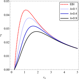
(a)  $q=1.5$ and $b=1.4$

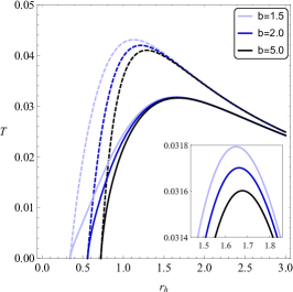
(b)  $q=1.5$ and $\lambda=0.4$

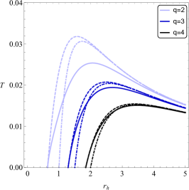
(c)  $b=1.3$ and $\lambda=0.8$

Figure 1: The behavior of $T$ versus $r_{h}$ for spherical asymptotically flat solutions with various values of $\lambda$, $b$ and $q$. Note that the solid (dashed) curves show the temperature in the presence (absence) of cubic terms. In the right panel, dot-dashed curves show the temperature for Einstein-Maxwell regime.

From Eqs. (40) and (41), we could determine $m$ and surface gravity $\kappa_{g}$ as functions of model parameters:

$$\kappa_{g}= \frac{r_{h}^{3}}{24\lambda k}\Bigg{[}1+\frac{12k\lambda b^{2}}{r_{h}^{2}}\left(1-\sqrt{1+\frac{q^{2}}{b^{2}r_{h}^{4}}}\right)$$

$$-\frac{24k\lambda\Lambda_{0}}{r_{h}^{2}}+\frac{24k^{2}\lambda}{r_{h}^{4}}\Bigg{]}^{\frac{1}{2}}-\frac{r_{h}^{3}}{24\lambda k},$$ (44)

$$\frac{m}{r_{h}} =k-\frac{24\lambda\kappa_{g}^{2}}{r_{h}^{2}}k-\frac{\Lambda_{0}r_{h}^{2}}{3}-\frac{16\lambda\kappa_{g}^{3}}{r_{h}}$$

$$+\frac{b^{2}r_{h}^{2}}{6}\left[1-\,\mathbf{F}\left(-\frac{1}{2},-\frac{3}{4},\frac{1}{4},-\frac{q^{2}}{b^{2}r_{h}^{4}}\right)\right].$$ (45)

It is notable to point out that $m$ is related to total mass $M$ via Eq. (33). If $\lambda$ and $b$ tends to zero and infinity, respectively, the above equations reduce to RN-(A)ds black hole ones:

$$\kappa_{g} =\frac{k}{2r_{h}}-\frac{q^{2}}{8r_{h}^{3}}-\frac{\Lambda_{0}r_{h}}{2},$$ (46)

$$\frac{m}{r_{h}} =k-\frac{\Lambda_{0}r_{h}^{2}}{3}+\frac{q^{2}}{4r_{h}^{2}}.$$ (47)

The Hawking temperature of our solution can be written in terms of surface gravity HawTemp

$$T=\frac{\kappa_{g}}{2\pi},$$ (48)

where $\kappa_{g}$ has been given in Eq. (44). Using (44) and (48), one could find the temperature as

$$T =\frac{r_{h}^{3}}{48\pi\lambda k}\Bigg{[}1+\frac{12k\lambda b^{2}}{r_{h}^{2}}\left(1-\sqrt{1+\frac{q^{2}}{b^{2}r_{h}^{4}}}\right)+\frac{24k^{2}\lambda}{r_{h}^{4}}\Bigg{]}^{\frac{1}{2}}$$

$$\text{\ \ \ }-\frac{r_{h}^{3}}{48\pi\lambda k},$$ (49)

where we set $\Lambda_{0}=0$. Note that, according to discussions presented in section III, we study thermodynamics of asymptotically flat solutions ($\Lambda=0$) with vanishing bare cosmological constant $\Lambda_{0}$.

Here, it is worthwhile to discuss about the allowed values of $k$ for asymptotically flat solutions. We know that for Einstein-Maxwell gravity case, the metric function of asymptotically flat topological solution is $f(r)=k-m/r+q^{2}/r^{2}$, which obviously does not present viable black holes if $k=0$ and $k=-1$ since that would imply a wrong sign for the metric for large values of radial coordinate $r$ where $-m/r$ or $-1$ would dominate. It is exactly the case for bare ECG because the contributions from the cubic piece are very small, asymptotically (for large $r$) as well. For the BI charged black holes in ECG, this reasoning holds since the term related to nonlinear electrodynamics in metric function (as appears in Eq. (11)) is asymptotically proportional to $r^{-2}$. So, we focus on spherically symmetric black hole solutions ($k=1$) because those are the only ones which could exist in asymptotically flat space. One also could check that in hyperbolic and planar cases, the temperature given by Eq. (49) is negative and from this point of view, as well, these cases are not physically meaningful. Therefore, we study the thermodynamics of asymptotically flat solutions with spherical topology on horizon.

Now, we are going to discuss the effects of each model parameter $\lambda$, $b$ and $q$ on the temperature of spherical asymptotically flat solutions. From Eq. (49), one can see that for $k=1$, the first term of temperature formula is positive while the second term is negative. Increasing parameters $b$ and $q$ enhances the magnitude of

$$\frac{12k\lambda b^{2}}{r_{h}^{2}}\left(1-\sqrt{1+\frac{q^{2}}{b^{2}r_{h}^{4}}}\right),$$

in Eq. (49). This term is negative for $k=1$, so, as $b$ or $q$ increases, the temperature $T$ of spherical asymptotically flat solutions decreases. In order to exhibit these effects, we have plotted $T$ versus $r_{h}$ for different values of $b$, $q$ and $\lambda$ in Fig. 1. This figure shows that as each one of parameters $b$, $q$ or $\lambda$ grows, the temperature value becomes lower. This means that as the effect of the cubic term grows (or equivalently, as the nonlinearity of electrodynamics weakens), the temperature of spherical black holes decreases. Fig. 1 shows that for spherical asymptotically flat solutions, there is a maximum temperature $T_{\text{max}}$.  The behavior of $T_{\text{max}}$ in terms of model parameters is exhibited in table 1 as well. One can find that the value of $T_{\text{max}}$ decreases as each of the parameters $\lambda$, $b$ and $q$ increases.

Table 1: The behavior of maximum temperature $T_{\text{max}}$ for various values of model parameters.

$\lambda$	$b$	$q$	$T_{\text{max}}$
0.01			0.10
0.02	0.2	0.5	0.08
0.05			0.06
	0.01		0.10
0.01	0.50	1	0.08
	0.95		0.07
		0.8	0.08
0.01	0.6	1.2	0.07
		1.6	0.06

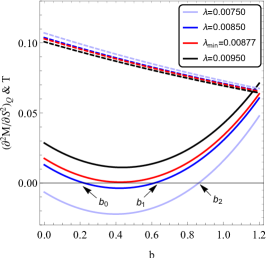
(a)  

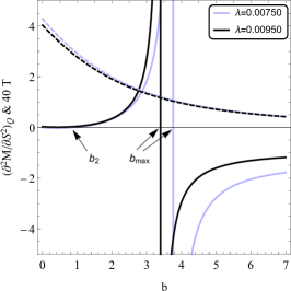
(b)  

Figure 2: The behaviors of $(\partial^{2}M/\partial S^{2})_{Q}$ and $T$ (dashed) versus $b$ for different values of $\lambda$ with $q=1$ and $r_{h}=0.5$.

Let us now calculate the entropy of our black holes. The entropy of black solutions in higher-order gravities could be computed by Wald’s formula given by entropy

$$S=-2\pi\int_{H}d^{2}x\sqrt{h}\frac{\delta\mathcal{L}_{G}}{\delta R_{abcd}}\epsilon_{ab}\epsilon_{cd}\,,$$ (50)

where $h$ is the determinant of the induced metric on the horizon, $\delta\mathcal{L}_{G}/\delta R_{abcd}$ is the Euler-Lagrange derivative of gravitational Lagrangian and $\epsilon_{ab}$ is the binormal of the horizon normalized as $\epsilon_{ab}\epsilon^{ab}=-2$. Applying the above formula on our theory introduced by action (1), we receive

$$S= \frac{1}{4}\int_{H}d^{2}x\sqrt{h}\Big{[}1+2\alpha_{2}R_{(2)}+\lambda\Big{(}36R_{b\ d}^{\ e\ f}R_{aecf}$$

$$+3R_{ab}^{\ \ ef}R_{cdef}-12R_{ac}R_{db}-24R^{ef}R_{ebfc}g_{bd}$$

$$+24g_{bd}R_{ce}R_{\ a}^{e}\Big{)}\epsilon^{ab}\epsilon^{cd}\Big{]}\,,$$ (51)

in which $R_{(2)}$ is the Ricci scalar of the induced metric on the horizon. This term comes from the Gauss-Bonnet term $L_{2}=R^{2}-4R_{ab}R^{ab}+R_{abcd}R^{abcd}$ in the action (1). As we have pointed out before, this term is topological and hence has no effect in our calculations so far. However, it contributes to the entropy. Using the metric (4) with $N=1$, one determines the entropy per unit area as

$$S=\frac{r_{h}^{2}}{4}\left[1-24\lambda\frac{\kappa_{g}^{2}}{r_{h}^{2}}\left(\frac{2k}{\kappa_{g}r_{h}}+1\right)\right]+k\alpha_{2}\,,$$ (52)

in which $\kappa_{g}$ could be replaced by Eq. (44). It is remarkable to mention that, the above relation reduces to $r_{h}^{2}/4$ adsbi1 if the higher-order terms disappear ($\lambda=\alpha_{2}=0$).

Now, we turn to calculate the electric potential. The electric potential $U$, measured at infinity with respect to horizon is defined by

$$U=A_{\mu}\chi^{\mu}\left|{}_{r\rightarrow\infty}-A_{\mu}\chi^{\mu}\right|_{r=r_{h}},$$ (53)

where $\chi=\partial_{t}$ is the null generator of the horizon. Using (9) and (53), one finds

$$U=\frac{q}{r_{h}}\,\mathbf{F}\left(\frac{1}{2},\frac{1}{4},\frac{5}{4},-\frac{q^{2}}{b^{2}r_{h}^{4}}\right).$$ (54)

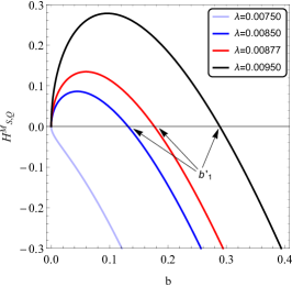
(a)  

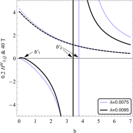
(b)  

Figure 3: The behavior of $\mathbf{H}_{S,Q}^{M}$ and $T$ (dashed) versus $b$ for different values of $\lambda$ with $q=1$ and $r_{h}=0.5$.

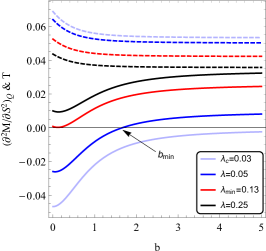
(a)  $(\partial^{2}M/\partial S^{2})_{Q}$ and $T$ vs $b$

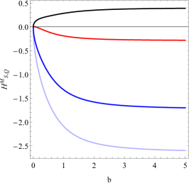
(b)  $\mathbf{H}_{S,Q}^{M}$ vs $b$

Figure 4: The behaviors of $(\partial^{2}M/\partial S^{2})_{Q}$, $\mathbf{H}_{S,Q}^{M}$ and $T$ (dashed) versus $b$ for different values of $\lambda$ with $q=1$ and $r_{h}=1$.

In order to check the first law of thermodynamics, we first write a Smarr-type formula. Using Eqs. (34), (37) and (45), the Smarr-type formula $M\left(r_{h},Q\right)$ can be written as

$$M\left(r_{h},Q\right) =\frac{1}{8\pi}\Bigg{[}kr_{h}-\frac{4\lambda\kappa_{g}^{2}}{r_{h}}\left(6k+4\kappa_{g}r_{h}\right)$$

$$+\frac{1}{6}b^{2}r_{h}^{3}\left(1-\,\mathbf{F}\left(-\frac{1}{2},-\frac{3}{4},\frac{1}{4},-\frac{\left(16\pi Q\right)^{2}}{b^{2}A_{k}^{2}r_{h}^{4}}\right)\right)\Bigg{]}.$$ (55)

According to Eq. (52), $r_{h}=r_{h}(S,Q)$ and in general $M=M(S,Q)$. We can then consider $S$ and $Q$ as a complete set of extensive quantities for mass. Therefore, temperature $T$ and electric potential $U$ are defined as conjugate intensive quantities for $S$ and $Q$, respectively and

$$T=\left(\frac{\partial M}{\partial S}\right)_{Q},\text{ \ \ \ \ }U=\left(\frac{\partial M}{\partial Q}\right)_{S}.$$

These intensive quantities can be calculated using Eqs. (37),  (52) and (55) where

$$T = \left(\frac{\partial M}{\partial S}\right)_{Q}=\left(\frac{\partial M}{\partial r_{h}}\right)_{Q}\left(\frac{\partial S}{\partial r_{h}}\right)_{Q}^{-1},$$ (56)

$$U = \left(\frac{\partial M}{\partial Q}\right)_{S}=\left(\frac{\partial M}{\partial Q}\right)_{r_{h}}+\left(\frac{\partial M}{\partial r_{h}}\right)_{Q}\left(\frac{\partial r_{h}}{\partial Q}\right)_{S}$$ (57)

$$= \left(\frac{\partial M}{\partial Q}\right)_{r_{h}}-\frac{\left(\frac{\partial S}{\partial Q}\right)_{r_{h}}\left(\frac{\partial M}{\partial r_{h}}\right)_{Q}}{\left(\frac{\partial S}{\partial r_{h}}\right)_{Q}}$$

$$= \left(\frac{\partial M}{\partial Q}\right)_{r_{h}}-T\left(\frac{\partial S}{\partial Q}\right)_{r_{h}}.$$

Our calculations show that $T$ and $U$ computed by Eqs. (56) and (57) coincide with ones obtained from Eqs. (49) and (54) for nonlinearly charged spherical ($k=1$) asymptotically flat solutions. Thus, the first law of thermodynamics

$$dM=TdS+UdQ,$$ (58)

is satisfied by these quantities.

In next section, we will study the thermal stability of spherical solutions in both canonical and grand canonical ensembles.

V Thermal stability

In this section, we intend to study thermal stability of the four-dimensional nonlinearly charged asymptotically flat solutions of ECG with spherical horizon in both canonical and grand canonical ensembles. In canonical ensemble where the charge is a fixed parameter, the positivity of heat capacity $C=T/(\partial T/\partial S)_{Q}=T/(\partial^{2}M/\partial S^{2})_{Q}$ guarantees the local stability stab . Therefore, it is sufficient to check that $(\partial^{2}M/\partial S^{2})_{Q}$ is positive in order to explore the stability of solutions in the ranges where temperature is positive as well. Charge $Q$ is no longer fixed in the grand canonical ensemble. In this ensemble, the system is locally stable provided that the determinant of Hessian matrix $\mathbf{H}_{S,Q}^{M}=\left[\partial^{2}M/\partial S\partial Q\right]$ is positive, in positive temperature ranges. Since the explicit forms of $(\partial^{2}M/\partial S^{2})_{Q}$ and $\mathbf{H}_{S,Q}^{M}$ are complicated, we avoid writing them here. However, the main results are depicted in Figs. 2-4.

Let us now turn to study the stability of black hole solutions in canonical and grand canonical ensembles. Our investigations show that the values of charge $q$ and horizon radius $r_{h}$ determine how thermal stability is influenced by the other parameters. We study thermal stability in canonical ensemble for two different types of solutions (Figs. 2 and 4(a)). Let us focus on the first type exhibited in Fig. 2. As Fig. 2(a) shows, in highly nonlinear electrodynamics regime (small nonlinearity parameter $b$ values), there is a minimum value for cubic coupling $\lambda$ ($\lambda_{\min}$) that for values greater than it, the system is stable up to $b_{\max}$ (Fig. 2(b)). For $\lambda$ values a bit smaller than $\lambda_{\min}$, the system is stable except for $b$ values between $b_{0}$ and $b_{1}$ (Fig. 2(a)). As $\lambda$ becomes smaller, $b_{0}$ tends to zero and $b_{1}$ becomes greater. So, the instability interval becomes larger. In this case, the system is stable for $b$ values between $b_{2}$ and $b_{\max}$ (Fig. 2(b)). $b_{2}$ and $b_{\max}$ increase as $\lambda$ decreases. Also, for $b$ values greater than $b_{\max}$ (including linear Maxwell case), the system is unstable. Note that we plot the curves in Fig. 2(b) just for two $\lambda$ values in order not to have a messy plot. For other $\lambda$ values, the qualitative behavior is the same. In addition, we plot the temperature in Figs. 2-4 as well, to ensure it is positive in the regions under study. One could see that the behavior of temperature in terms of $\lambda$ and $b$ coincides with what we have discussed before i.e. temperature decreases as each of the latter parameters increases. In second type displayed in Fig. 4(a), we again have a minimum value for $\lambda$. However, in this case, there is no upper bound for $b$ and the system is stable for all $b$ values if $\lambda\geq\lambda_{\min}$. For $\lambda$ values a bit smaller than $\lambda_{\min}$, there is a minimum value for $b$ ($b_{\min}$) as well, that for $b>b_{\min}$, we have a stable system. As $\lambda$ becomes smaller, we have a critical value $\lambda_{c}$ that for $\lambda<\lambda_{c}$, the system is unstable for all $b$ values.

We continue by discussing the thermal stability in grand canonical ensemble. For the first type represented in Fig. 3, in highly nonlinear electrodynamics regime (Fig. 3(a)), the system is unstable for some cubic couplings, however for some greater ones, the system becomes stable up to a specific value of $b$ ($b_{1}^{\prime}$). For $b$ values greater than $b_{1}^{\prime}$, we have an unstable system between $b_{1}^{\prime}$ and $b_{2}^{\prime}$ (Fig. 3(b)). For $b>b_{2}^{\prime}$ (including linear Maxwell case), the system becomes thermally stable. $b_{1}^{\prime}$ ($b_{2}^{\prime}$) is greater (smaller) for greater values of $\lambda$. In second type displayed in Fig. 4(b), whereas the system is unstable for some values of $\lambda$, it becomes totally stable as $\lambda$ grows.

VI Summary and concluding remarks

In the present paper, we studied four-dimensional topological Born-Infeld (BI) charged black hole solutions in the context of Einsteinian cubic gravity (ECG) in the presence of a bare cosmological constant. ECG is the most general gravity up to cubic order in curvature which is independent of dimension and its linearized spectrum coincides with general relativity one. Also, both theoretical (open superstring theory) and experimental (photon-photon interaction experiments) evidences suggest nonlinear theories of electrodynamics such as BI model. On the other hand, topological black hole solutions are known to be dual to some thermal states in the holographic settings, with quite different thermodynamical features depending on the specific topology. To the best of our knowledge, this is the first study of topological black hole solutions in ECG with nonlinear electrodynamics.

We first introduced the action of the theory and obtained its corresponding field equations. Integrating these field equations, we obtained the electromagnetic potential as well as a second order differential equation for the metric function. Then, we presented the total mass $M$ formula by employing Abbott-Deser-Tekin method and showed that the total mass depends on cubic coupling in general. We obtain the total charge $Q$ via Gauss formula as well. Moreover, we discussed the conditions under which the model is unitary and perturbatively ghost-free and explored different possible cases. We found that if the bare cosmological constant vanishes, then the model is unitary only if the solution is asymptotically flat. Therefore, we focused on studying the thermodynamics of asymptotically flat solutions. These are necessarily of spherical topology. Expanding the metric function at the near horizon region up to second order in the field equations, we obtained the temperature $T$ and the total mass as functions of horizon radius $r_{h}$ and charge $q$. Next, we revealed the influences of cubic coupling $\lambda$, nonlinearity parameter $b$ and black hole charge on the behavior of the temperature. We found that the temperature decreases as the values of these parameters increase. It is remarkable to mention that, as $b$ grows, the linear Maxwell electrodynamics is reproduced. In addition, the temperature of spherical asymptotically flat solutions have a maximum value as horizon radius changes. This maximum temperature is smaller for greater values of $\lambda$, $b$ and $q$. In order to check the satisfaction of thermodynamics first law, we turned to compute the entropy and the electric potential. We used the Wald formula in order to obtain the entropy of our solutions. We showed that the first law of thermodynamics is satisfied for spherical BI charged asymptotically flat solutions of ECG.

Finally, we analysed thermal stability of our solutions in both canonical and grand canonical ensembles. We showed that the values of $q$ and $r_{h}$ specify how the stability is affected by other parameters, in both ensembles. For one type of solutions, the system is unstable for $b$ values larger than a maximum value $b_{\max}$ (including linear Maxwell case) in canonical ensemble. In the small $b$ regime (highly nonlinear electrodynamics), there is also a minimum $\lambda$ value. The system is stable if $\lambda\geq\lambda_{\min}$ for $b$ in the range $0$ to $b_{\max}$. There exists another type of solution with $\lambda_{\min}$ defined as before, but in which, black solutions are stable if $\lambda\geq\lambda_{\min}$ with no upper bound for $b$. Furthermore, for $\lambda$ values a bit smaller than $\lambda_{\min}$, the system is stable for $b>b_{\min}$. There is also a critical value for $\lambda$ that if $\lambda<\lambda_{c}$, the black hole solutions are thermally unstable for all $b$ values. In grand canonical ensemble, the first type system is stable for large $b$ values (including linear Maxwell case). Nevertheless, in small $b$ regime, it is unstable for some $\lambda$ values. In this regime, the system becomes stable for $b$ values between $0$ and an upper bound, as $\lambda$ grows. The second type system, in grand canonical ensemble, is totally unstable for some $\lambda$ values. However, it becomes totally stable, as $\lambda$ increases.

In the present work, we focused on asymptotically flat solutions with vanishing bare cosmological constant according to discussions given in Sec. III. In such a scenario, the higher curvature terms have no contribution in the total mass formula. However, if one considers possible (A)dS vacuum solutions in a unitary model, a correction due to cubic curvature terms appears in the total mass formula (see Eq. (33)). This fact may affect the thermdoynamical studies, drastically. It is fascinating to explore these kinds of charged solutions in future works. In addition, here, we considered Born-Infeld model as nonlinear electrodynamics. It is interesting to study the effects of other known nonlinear models of electrodynamics on ECG solutions. Moreover, it is worthwhile to explore the critical behavior of nonlinearly charged solutions of ECG in both extended ext and non-extended nonext thermodynamics phase spaces. Some of these issues are under investigation and the results will appear elsewhere.

Appendix A Calculation of $\mathcal{P}$

Here, we present the detailed calculations for obtaining $\mathcal{P}$ in Eq. (15). From Eq. (2), we have

$$\mathcal{P}= 12R_{a\ b}^{\ c\ d}R_{c\ d}^{\ e\ f}R_{e\ f}^{\ a\ b}+R_{ab}^{cd}R_{cd}^{ef}R_{ef}^{ab}$$

$$-12R_{abcd}R^{ac}R^{bd}+8R_{a}^{b}R_{b}^{c}R_{c}^{a}\,.$$ (59)

The above equation, can be re-written as

$$\mathcal{P}= 12R^{acbd}R_{cedf}R_{a\text{ }b}^{\text{ }e\text{ }f}+R_{ab}^{cd}R_{cd}^{ef}R_{ef}^{ab}$$

$$-12R_{cd}^{ab}R_{a}^{c}R_{b}^{d}+8R_{a}^{b}R_{b}^{c}R_{c}^{a}\,.$$ (60)

Then, using

$$R^{acbd}R_{cedf}R_{a\text{ }b}^{\text{ }e\text{ }f}=R^{acbd}R_{a\text{ }b}^{\text{ }e\text{ }f}R_{cfde}+\frac{1}{4}R^{acbd}R_{ac}^{\text{ \ \ \ }ef}R_{bdef},$$

Eq. (60) can be expressed as

$$\mathcal{P}= 12R^{acbd}R_{a\text{ }b}^{\text{ }e\text{ }f}R_{cfde}+3R^{acbd}R_{ac}^{\text{ \ \ \ }ef}R_{bdef}+R_{ab}^{cd}R_{cd}^{ef}R_{ef}^{ab}$$

$$-12R_{cd}^{ab}R_{a}^{c}R_{b}^{d}+8R_{a}^{b}R_{b}^{c}R_{c}^{a}\,.$$ (61)

Rearranging the above equation yields

$$\mathcal{P}= 12R_{cd}^{ab}R_{af}^{ce}R_{be}^{df}+4R_{cd}^{ab}R_{ab}^{ef}R_{ef}^{cd}$$

$$-12R_{cd}^{ab}R_{a}^{c}R_{b}^{d}+8R_{b}^{a}R_{a}^{c}R_{c}^{b}\,,$$ (62)

which is what we expressed in Eq. (15).

References

- (1) B. P. Abbott, et al. (LIGO Scientific Collaboration, Virgo Collaboration), Observation of gravitational waves from a binary black hole merger, Phys. Rev. Lett. 116, 061102 (2016), [arXiv:1602.03837].
- (2) D. Lovelock, Divergence-free tensorial concomitants, Aequationes mathematicae 4, 127 (1970).
- (3) D. Lovelock, The Einstein Tensor and Its Generalizations, J. Math. Phys. (N.Y.) 12, 498 (1971).
- (4) P. Bueno and P. A. Cano, Einsteinian cubic gravity, Phys. Rev. D 94, 104005 (2016), [arXiv:1607.06463].
- (5) A. Dey, P. Roy, and T. Sarkar, On holographic Renyi entropy in some modified theories of gravity, J. High Energy Physics 04, 098 (2018), [arXiv:1609.02290].
- (6) R. A. Hennigar and R. B. Mann, Black holes in Einsteinian cubic gravity, Phys. Rev. D 95, 064055 (2017), [arXiv:1610.06675].
- (7) P. Bueno and P. A. Cano, Four-dimensional black holes in Einsteinian cubic gravity, Phys. Rev. D 94, 124051 (2016), [arXiv:1610.08019].
- (8) R. A. Hennigar, D. Kubiznak, and R. B. Mann, Generalized quasitopological gravity, Phys. Rev. D 95, 104042 (2017), [arXiv:1703.01631].
- (9) P. Bueno and P. A. Cano, On black holes in higher-derivative gravities, Class. Quant. Grav. 34, 175008 (2017), [arXiv:1703.04625].
- (10) P. Bueno and P. A. Cano, Universal black hole stability in four dimensions, Phys. Rev. D 96, 024034 (2017), [arXiv:1704.02967].
- (11) R. A. Hennigar, M. B. J. Poshteh, and R. B. Mann, Shadows, Signals, and Stability in Einsteinian Cubic Gravity, Phys. Rev. D 97, 064041 (2018), [arXiv:1801.03223].
- (12) P. Bueno, P. A. Cano, and A. Ruiperez, Holographic studies of Einsteinian cubic gravity, J. High Energy Physics 03, 150 (2018), [arXiv:1802.00018].
- (13) P. Bueno, P. A. Cano, R. A. Hennigar, and R. B. Mann, NUTs and bolts beyond Lovelock, J. High Energy Physics 10, 095 (2018), [arXiv:1808.01671].
- (14) Y.-Z. Li, Holographic Studies of The Generic Massless Cubic Gravities, Phys. Rev. D 99, 066014 (2019), [arXiv:1901.03349].
- (15) M. R. Mehdizadeh and A. H. Ziaie, Traversable wormholes in Einsteinian cubic gravity, Modern Physics Letters A, 2050017 (2019), [arXiv;1903.10907].
- (16) P. Bueno, P. A. Cano, and R. A. Hennigar, (Generalized) quasi-topological gravities at all orders, Class. Quant. Grav. 37, 015002 (2020), [arXiv:1909.07983].
- (17) P. A. Cano and D. Pereiguez, Extremal Rotating Black Holes in Einsteinian Cubic Gravity, Phys. Rev. D 101 , 044016 (2020), [arXiv:1910.10721].
- (18) D. J. Burger, W. T. Emond, and N. Moynihan, Rotating Black Holes in Cubic Gravity, Phys. Rev. D 101 , 084009 (2020), [arXiv:1910.11618].
- (19) A. M. Frassino and J. V. Rocha, Charged black holes in Einsteinian cubic gravity and non-uniqueness, [arXiv:2002.04071].
- (20) M. Born and L. Infeld, Foundations of the new field theory, Proc. R. Soc. A 144, 425 (1934).
- (21) E. S. Fradkin and A. A. Tseytlin, Effective field theory from quantized string, Phys. Lett. B 163, 123 (1985).
- (22) R. R. Metsaev, M. A. Rakhmanov and A. A. Tseytlin, The Born-Infeld action as the effective action in the open superstring theory, Phys. Lett. B 193, 207 (1987).
- (23) E. Bergshoeff, E. Sezgin, C. Pope and P. Townsend, The Born-lnfeld action from conformal invariance of the open superstring, Phys. Lett. B 188, 70 (1987).
-
(24)
D. L. Burke et al., Positron Production in Multiphoton
Light-by-Light Scattering, Phys. Rev. Lett. 79, 1626 (1997);
C. Bamber et al., Studies of nonlinear QED in collisions of 46.6-GeV electrons with intense laser pulses, Phys. Rev. D 60, 092004 (1999);
D.Tommasini, A. Ferrando, H. Michinel and M.Seco, Detecting photon-photon scattering in vacuum at exawatt lasers, Phys. Rev. A 77, 042101 (2008) , [arXiv:0802.0101];
D. Tommasini, A. Ferrando, H. Michinel and M. Seco, Precision tests of QED and non-standard models by searching photon-photon scattering in vacuum with high power lasers, J. High Energy Phys. 0911, 043 (2009), [arXiv:0909.4663];
O. J. Pike, F. Mackenroth, E. G. Hill and S. J. Rose, A photon–photon collider in a vacuum hohlraum, Nature Photonics 8, 434 (2014). - (25) D. Birmingham, Topological Black Holes in Anti-de Sitter Space, Class. Quant. Grav. 16, 1197 (1999), [hep-th/9808032].
- (26) R. Emparan, AdS/CFT Duals of Topological Black Holes and the Entropy of Zero-Energy States, J. High Energy Physics 9906, 036 (1999), [hep-th/9906040].
- (27) A. Sheykhi, Topological Born-Infeld-dilaton black holes, Phys. Lett. B 662, 7 (2008), [arXiv:0710.3827].
- (28) T. K. Dey, Born-Infeld black holes in the presence of a cosmological constant, Phys. Lett. B 595, 484 (2004), [hep-th/0406169]; R. G. Cai, D. W. Pang and A. Wang, Born-Infeld Black Holes in (A)dS Spaces, Phys. Rev. D 70, 124034 (2004), [hep-th/0410158]; D. C. Zou, Z. Y. Yang, R. H. Yue and P. Li, Thermodynamics of Gauss-Bonnet-Born-Infeld black holes in AdS space, Mod. Phys. Lett. A 26, 515 (2011), [arXiv:1011.3184]; P. Li, R. H. Yue and D. C. Zou, Thermodynamics of Third Order Lovelock-Born-Infeld Black Holes, Commun. Theor. Phys. 56, 845 (2011), [arXiv:1110.0064].
-
(29)
S. Deser and B. Tekin, Gravitational energy in quadratic
curvature gravities, Phys. Rev. Lett. 89, 101101 (2002), [hep-th/0205318];
S. Deser and B. Tekin, Energy in generic higher curvature gravity theories, Phys. Rev. D 67, 084009 (2003), [hep-th/0212292];
L. F. Abbott and S. Deser, Stability of gravity with a cosmological constant, Nucl. Phys. B 195, 76 (1982). -
(30)
T. C. Sisman, I. Gullu and B. Tekin, All unitary cubic
curvature gravities in D dimensions, Class. Quant. Grav. 28, 195004 (2011), [arXiv:1103.2307];
C. Senturk, T. C. Sisman and B. Tekin, Energy and Angular Momentum in Generic F(Riemann) Theories, Phys. Rev. D 86, 124030 (2012), [arXiv:1209.2056];
H. Adami, M. R. Setare, T. C. Sisman and B. Tekin, Conserved Charges in Extended Theories of Gravity,Phys. Rept. 834, 1 (2019), [arXiv:1710.07252]. - (31) S. A. Fulling, R. C. King, B. G. Wybourne and C. J. Cummins, Normal forms for tensor polynomials. I. The Riemann tensor, Class. Quant. Grav. 9, 1151 (1992).
- (32) S. W. Hawking, Black hole explosions?, Nature 248, 30 (1974).
- (33) R. M. Wald, Black Hole Entropy is Noether Charge, Phys. Rev. D 48, 3427 (1993), [gr-qc/9307038]; V. Iyer and R. M. Wald, Some Properties of Noether Charge and a Proposal for Dynamical Black Hole Entropy, Phys. Rev. D 50, 846 (1994), [gr-qc/9403028]; T. Jacobson, G. Kang and R. C. Myers, On Black Hole Entropy, Phys. Rev. D 49, 6587 (1994), [gr-qc/9312023].
-
(34)
M. Cvetic and S. S. Gubser, Phases of R-charged Black Holes,
Spinning Branes and Strongly Coupled Gauge Theories, J. High Energy Phys. 04, 024 (1999), [hep-th/9902195];
M. M. Caldarelli, G. Cognola and D. Klemm, Thermodynamics of Kerr-Newman-AdS
Black Holes and Conformal Field Theories, Class. Quant. Gravit. 17, 399 (2000), [hep-th/9908022];
S. S. Gubser and I. Mitra, The evolution of unstable black holes in anti-de Sitter space, J. High Energy Phys., 08, 018 (2001). - (35) D. Kubiznak and R. B. Mann, P-V criticality of charged AdS black holes, J. High Energy Physics 1207, 033 (2012), [arXiv:1205.0559].
- (36) A. Dehyadegari, A. Sheykhi and A. Montakhab, Critical behaviour and microscopic structure of charged AdS black holes via an alternative phase space, Phys. Lett. B 768, 235 (2017), [arXiv:1607.05333].