${\cal N}=4$ SYM Quantum Spectral Curve in BFKL regime

Abstract

We review the applications of the Quantum Spectral Curve (QSC) method to the Regge (BFKL) limit in $\mathcal{N}=4$ supersymmetric Yang-Mills theory. QSC, based on quantum integrability of the AdS₅/CFT₄ duality, was initially developed as a tool for the study of the spectrum of anomalous dimensions of local operators in the $\mathcal{N}=4$ SYM in the planar, $N_{c}\to\infty$ limit. We explain how to apply the QSC for the BFKL limit, which requires non-trivial analytic continuation in spin $S$ and extends the initial construction to non-local light-ray operators. We give a brief review of high precision non-perturbative numerical solutions and analytic perturbative data resulting from this approach. We also describe as a simple example of the QSC construction the leading order in the BFKL limit. We show that the QSC substantially simplifies in this limit and reduces to the Faddeev-Korchemsky Baxter equation for Q-functions. Finally, we review recent results for the Fishnet CFT, which carries a number of similarities with the Lipatov’s integrable spin chain for interacting reggeized gluons.

1 Introduction

The Balitsky-Fadin-Kuraev-Lipatov (BFKL) approximation Kuraev:1977fs ; Balitsky:1978ic in Quantum Chromodynamics (QCD) has marked the beginning of a new era in the study of the properties of hadron collisions at high energy. Among various important results following BFKL approach, the Pomeron spectrum was calculated in the leading Kuraev:1977fs ; Balitsky:1978ic ; Lipatov:1985uk , and then, 20 years later, in the next-to-leading Fadin:1998py logarithmic approximations (LO and NLO). The complexity of the conventional Feynman perturbation theory increases dramatically at each order and it is unlikely that the NNLO calculation in QCD is reachable with the currently available techniques.

The history of integrability in gauge theories starts from the renowned Lev Lipatov’s work Lipatov:1993yb , where the effective Lagrangian for reggeized gluons in QCD was shown to be integrable. Lipatov was also the first to notice the equivalence of this system to the $SL(2,\mathbb{C})$ integrable quantum spin chain Lipatov:1993qn . Following the seminal paper Faddeev:1994zg , the integrability approach to Lipatov’s model has been substantially advanced in Derkachov:2001yn ; DeVega:2001pu ; Derkachov:2002wz ; Derkachov:2002pb .

The BFKL approximation was then successfully applied to the study of the spectrum of anomalous dimensions of certain operators in $\mathcal{N}=4$ SYM theory Kotikov:2000pm . The result of this calculation appears to be slightly less complex than the original Regge limit in QCD, possibly due to the super-symmetry. As it was noticed in Kotikov:2000pm ; Kotikov:2002ab the result follows the so-called maximal transcendentality selection principle – only the most complicated in transcedentality parts of the QCD result are present in its $\mathcal{N}=4$ SYM counterpart, with exactly the same coefficients. Even in this, maximally super-symmetric theory the complexity of the traditional Feynman perturbation technique increases factorially at each order. However, a powerful alternative method is available in this theory: due to the quantum integrability of planar $\mathcal{N}=4$ SYM theory it became possible to compute the spectrum of the planar $\mathcal{N}=4$ SYM theory at any value of the ’t Hooft coupling $\lambda=16\pi^{2}g^{2}=g_{YM}^{2}N_{c}$! This integrability was discovered at one loop in the seminal Minahan-Zarembo paper Minahan:2002ve  , then it was demonstrated at two-loops Beisert:2003tq , then at strong coupling in Bena:2003wd ; Kazakov:2004qf ; Beisert:2005bm , via AdS/CFT correspondence, then generalized up to wrapping order in  Janik:2006dc ; Beisert:2005if ; Beisert:2006ez ; Ambjorn:2005wa , and finally to all loops, first in terms of the exact Y-system Gromov:2009bc , and then of the TBA equations Bombardelli:2009ns ; Gromov:2009tv ; Arutyunov:2009ur for the simplest Konishi-like operators. A few years ago, this line of research resulted in the final formulation of the solution of the spectral problem – the Quantum Spectral Curve (QSC) of the AdS₅/CFT₄ duality Gromov:2014caa ; Gromov:2015dfa .

The QSC equations can be formulated as a finite system of Riemann-Hilbert-type equations on 4+4 Baxter Q-functions. The QSC formalism has led to the tremendous progress in high precision numerical and multi-loop computations in a multitude of particular physical quantities (see the reviews Gromov:2017blm ; Kazakov:2018hrh and citations therein). Notably, the dimension $\Delta$ of twist-2 operator of the type ${\rm tr}(Z\nabla_{+}^{S}Z)$ was computed for virtually arbitrary coupling and arbitrary complex values of spin $S$ Gromov:2015wca  (see the Figure 1 and Figure 2). The particular corner of this picture, when $S\simeq-1+{\cal O}(g^{2})$ at weak coupling $g^{2}\to 0$, corresponds to the BFKL regime. The loop expansion of $S$ can be written as follows

$$S=-1+g^{2}\chi_{\textrm{LO}}(\Delta)+g^{4}\chi_{\textrm{NLO}}(\Delta)+g^{6}\chi_{\textrm{NNLO}}(\Delta)+g^{8}\chi_{\textrm{NNNLO}}(\Delta)+\mathcal{O}(g^{8})\;,$$ (1)

where $\chi_{\textrm{N}^{k}\textrm{LO}}(\Delta)$ is the BFKL kernel eigenvalue at the $(k+1)$-st loop. The BFKL limit of QSC was first explored in Alfimov:2014bwa and the LO BFKL spectrum $\chi_{\textrm{LO}}(\Delta)$ with zero conformal spin was reproduced there. The coefficient $\chi_{\textrm{NLO}}(\Delta)$ calculated in Kotikov:2000pm was successfully reproduced by the QSC calculations in Gromov:2015vua . Then, significant progress was made in the same work Gromov:2015vua , where QSC allowed to derive the NNLO BFKL kernel eigenvalue $\chi_{\textrm{NNLO}}(\Delta)$, which was later confirmed by the other method in Caron-Huot:2016tzz . It should be noted that all the BFKL kernel eigenvalues up to NNLO included can be written in terms of nested harmonic sums and multiple zeta values. Moreover, the high precision QSC numerical technique Gromov:2015wca is currently adapted in Alfimov:2018cms : for any order $\chi_{\textrm{N}^{k}\textrm{LO}}(\Delta)$ can be analyzed by the QSC numerical algorithm. Moreover, the QSC approach allowed to compute anomalous dimensions of the length-2 operators with both non-zero spins, including the conformal one $n$, ${\rm tr}(Z\nabla_{+}^{S}\nabla_{\perp}^{n}Z)$ Alfimov:2018cms .

In this short review, we give a concise formulation of the QSC and its reduction in the case of BFKL limit. We will briefly review the ideas of numerical and perturbative approaches to the solution of the QSC equations. We also shortly describe the most important numerical and perturbative analytic results for the BFKL limit of $\mathcal{N}=4$ SYM theory.

The BFKL also gave an inspiration for a number of other research directions over the years. In particular, we will explain here how the BFKL limit influenced the currently being actively developed so-called fishnet conformal field theory (FCFT) proposed in Gurdogan:2015csr as a double scaling limit combining weak coupling and strong $gamma$-deformation of $\mathcal{N}=4$ SYM  theory. Fishnet CFT attracted much of attention in the last few years Caetano:2016ydc ; Chicherin:2017cns ; Gromov:2017cja ; Chicherin:2017frs ; Grabner:2017pgm ; Mamroud:2017uyz ; Kazakov:2018qez ; Karananas:2019fox ; Gromov:2018hut ; Derkachov:2018rot ; Kazakov:2018gcy ; Basso:2018cvy ; Korchemsky:2018hnb ; Chowdhury:2019hns ; Gromov:2019jfh ; Basso:2019xay ; Derkachov:2019tzo ; Adamo:2019lor ; deMelloKoch:2019ywq ; Pittelli:2019ceq. It was generalized to any dimension $D$ Kazakov:2018qez , and for $D=2$ and a specific representation for conformal spins this model can be identified (for certain physical quantities) with the Lipatov’s $SL(2,\mathbb{R})$ spin chain for LO approximation of BFKL. As Fishnet CFT has a significant interplay with the initial ideas of BFKL integrability, we briefly review here the construction and integrability properties of fishnet CFT.

2 Integrability in $\mathcal{N}=4$ SYM

In the present Section we briefly review the integrable structure of $\mathcal{N}=4$ SYM. We connect the BFKL kernel eigenvalues to the dimensions of the twist-2 operators following Kotikov:2000pm , which allows us to apply the QSC to the study of the BFKL spectrum. This step requires certain generalisation of the gluing condition in QSC for the local operators, allowing for non-integer spins. As an example we demonstrate how to reproduce the Baxter equation, which initially appeared in the problem of diagonalization of the LO BFKL kernal.

2.1 BFKL spectrum and maximal transcendentality principle

Let us start from briefly describing the relation of the BFKL spectrum in $\mathcal{N}=4$ SYM to those in QCD. The key statement governing this connection is the so-called principle of maximal transcendentality Kotikov:2000pm ; Kotikov:2002ab . One can find a detailed description of this principle in Kotikov:2019xyg . Below we demonstrate this principle in application to the BFKL kernel eigenvalues. In what follows we use the extension of the formula (1) for the case of non-zero conformal spin $n$

$$S = -1+g^{2}\chi_{\textrm{LO}}(\Delta,n)+g^{4}\chi_{\textrm{NLO}}(\Delta,n)+$$

$$+ g^{6}\chi_{\textrm{NNLO}}(\Delta,n)+g^{8}\chi_{\textrm{NNNLO}}(\Delta,n)+\mathcal{O}(g^{10})\;.$$

Consider first the LO BFKL Pomeron kernel eigenvalues for QCD and $\mathcal{N}=4$ SYM  which can be found in Kuraev:1977fs ; Balitsky:1978ic and Kotikov:2000pm respectively. We see that the answers are identical and are given by

$$\chi_{\textrm{LO}}(\Delta,n)=-4\left(\psi\left(\frac{1+n+\Delta}{2}\right)+\psi\left(\frac{1+n-\Delta}{2}\right)-2\psi(1)\right)\;,$$ (3)

where $\Delta$ is the dimension of the state and $n$ is the conformal spin. Moreover, in the LO the BFKL kernel eigenvalues coincide for all 4D gauge theories Kotikov:2000pm .

For the next order in perturbation theory the situation is more subtle. The NLO BFKL kernel eigenvalue for QCD was calculated in Fadin:1998py

$$\chi_{\textrm{NLO}}^{\textrm{QCD}}(\Delta,n)=4\left[-2\Phi\left(n,\frac{1-\Delta}{2}\right)-2\Phi\left(n,\frac{1+\Delta}{2}\right)+6\zeta(3)+\right.$$

$$+ \left(\frac{67}{9}-2\zeta(2)-\frac{10n_{f}}{9N_{c}}\right)\frac{\chi_{\textrm{LO}}(\Delta,n)}{4}+\psi^{\prime\prime}\left(\frac{1+n-\Delta}{2}\right)+\psi^{\prime\prime}\left(\frac{1+n+\Delta}{2}\right)-$$

$$- \frac{1}{2}\left(\frac{11}{3}-\frac{2}{3}\frac{n_{f}}{N_{c}}\right)\left(\frac{\chi_{\textrm{LO}}^{2}(\Delta,n)}{16}-\psi^{\prime}\left(\frac{1+n+\Delta}{2}\right)+\psi^{\prime}\left(\frac{1+n-\Delta}{2}\right)\right)+$$

$$+ \frac{\pi^{2}\cos\frac{\pi(1+\Delta)}{2}}{\Delta\sin^{2}\frac{\pi(1+\Delta)}{2}}\left.\left(\left(3+\left(1+\frac{n_{f}}{N_{c}^{3}}\right)\frac{3\Delta^{2}-11}{4(\Delta^{2}-4)}\right)\delta^{0}_{n}-\left(1+\frac{n_{f}}{N_{c}^{3}}\right)\frac{\Delta^{2}-1}{8(\Delta^{2}-4)}\delta^{2}_{n}\right)\right]\;,$$

where $N_{c}$ is the number of colors and $n_{f}$ is the number of flavours of the fermions in the considered version of QCD. The same quantity in $\mathcal{N}=4$ SYM was first presented in Kotikov:2000pm . We write it down here from Kotikov:2002ab

$$\chi_{\textrm{NLO}}^{\mathcal{N}=4}(\Delta,n) = 4\left[-2\Phi\left(n,\frac{1-\Delta}{2}\right)-2\Phi\left(n,\frac{1+\Delta}{2}\right)+6\zeta(3)+\right.$$

$$+ \left.\frac{1}{4}\left(\frac{1}{3}-2\zeta(2)\right)\chi_{\textrm{LO}}(\Delta,n)+\psi^{\prime\prime}\left(\frac{1+n-\Delta}{2}\right)+\psi^{\prime\prime}\left(\frac{1+n+\Delta}{2}\right)\right]\;.$$

The function $\Phi(n,x)$ in the eigenvalues (2.1) and (2.1) is equal to

$$\Phi(n,x) = \sum\limits_{k=0}^{\infty}\frac{(-1)^{k+1}}{k+x+n/2}\left[\psi^{\prime}(k+n+1)-\psi^{\prime}(k+1)+(-1)^{k+1}(\beta^{\prime}(k+n+1)+\right.$$ (6)

$$+ \left.\beta^{\prime}(k+1))+\frac{1}{k+x+n/2}\left(\psi(k+n+1)-\psi(k+1)\right)\right]$$

and

$$\beta^{\prime}(z)=\frac{1}{4}\left[\psi^{\prime}\left(\frac{z+1}{2}\right)-\psi^{\prime}\left(\frac{z}{2}\right)\right]=\sum_{k=0}^{+\infty}\frac{(-1)^{k+1}}{(z+k)^{2}}\;.$$ (7)

Now we are going to explain the maximal transcendentality principle with the example of NLO BFKL kernel eigenvalue. There is a way to rewrite both $\chi_{\textrm{LO}}(\Delta,n)$ (3) and $\chi_{\textrm{NLO}}(\Delta,n)$ for both QCD (2.1) and $\mathcal{N}=4$ SYM (2.1) in terms of nested harmonic sums. In the LO we get simple result

$$\chi_{\textrm{LO}}(\Delta,n)=-4\left(S_{1}\left(\frac{1+\Delta+n}{2}-1\right)+S_{1}\left(\frac{1+n-\Delta}{2}-1\right)\right)\;,$$ (8)

from which we see that the LO BFKL kernel eigenvalues in QCD and $\mathcal{N}=4$ SYM have transcendentality $1$, where the transcendentality of a harmonic sum $S_{n_{1},\dots,n_{m}}$ is defined to be $|n_{1}|+\dots+|n_{m}|$, transcendentality of a product is given by a sum of the transcendentalities of the multipliers. In the same way one defines the transcendentality of the MZV $\zeta_{n_{1},\dots,n_{m}}$, which is given by the sum $n_{1}+\dots+n_{m}$. In particular, $\pi$ and $\log 2$ have transcedentality $1$.

To express (2.1) and (2.1) through nested harmonic sums we need to introduce some additional formulas. In Costa:2012cb it was shown, that for $n=0$ we can represent the NLO BFKL kernel eigenvalue for $\mathcal{N}=4$ SYM as follows

$$\chi_{\textrm{NLO}}^{\mathcal{N}=4}(\Delta,0)=F_{2}\left(\frac{1+\Delta}{2}\right)+F_{2}\left(\frac{1-\Delta}{2}\right)\;,$$ (9)

where

$$F_{2}(x) = 4\left(-\frac{3}{2}\zeta(3)+\pi^{2}\log 2+\frac{\pi^{2}}{3}S_{1}(x-1)+\right.$$

$$+ \left.\pi^{2}S_{-1}(x-1)+2S_{3}(x-1)-4S_{-2,1}(x-1)\right)\;.$$

Utilizing (9) and (2.1), we are able to rewrite (2.1) in the following way

$$\chi_{\textrm{NLO}}^{\mathcal{N}=4}(\Delta,n) = \frac{1}{2}\left(F_{2}\left(\frac{1+\Delta+n}{2}\right)+F_{2}\left(\frac{1-\Delta-n}{2}\right)+F_{2}\left(\frac{1+\Delta-n}{2}\right)+\right.$$ (11)

$$+ \left.F_{2}\left(\frac{1-\Delta+n}{2}\right)\right)+4\left(R_{n}\left(\frac{1-\Delta}{2}\right)+R_{n}\left(\frac{1+\Delta}{2}\right)\right)\;,$$

where

$$R_{n}(\gamma)=-8\left(S_{-2}\left(\gamma+\frac{n}{2}-1\right)+\frac{\pi^{2}}{12}\right)\left(S_{1}\left(\gamma+\frac{n}{2}-1\right)-S_{1}\left(\gamma-\frac{n}{2}-1\right)\right)\;.$$ (12)

Therefore, from (8), (9), (2.1), (11) and (12) we see that all the contributions to (11) have transcendentality $3$. Furthermore, we see that all the terms of the QCD result with the maximal transcendentality $3$ coincide exactly with the result of $\mathcal{N}=4$ SYM !

In the next part we will explain the relation of the BFKL kernel eigenvalues to the spectrum of length-2 (twist-2 in the case of zero conformal spin) operators in $\mathcal{N}=4$ SYM. Then we will explain how to adapt the QSC for the local operators to describe non-integer spin and conformal spin, which would then lead to the BFKL kernel eigenvalue.

2.2 Analytic structure of the twist-2 operator anomalous dimensions

In this part we describe the analytic structure of the length-2 operators with conformal spin in $\mathcal{N}=4$ SYM. Namely, we restrict ourselves to the states with the quantum numbers $J_{1}=2$, $J_{2}=J_{3}=0$. Let us first consider the case of zero conformal spin $S_{2}=0$, which are called the twist-2 $\mathfrak{sl}(2)$ operators

$$\mathcal{O}=\textrm{tr}ZD_{+}^{S}Z+(\textrm{permutations})\;.$$ (13)

In the gauge theory the physical operators should have even number of derivatives to be conformal primaries. The dimensions of these physical operators $\Delta$ were calculated for arbitrary even integer $S$ up to several loops order Lipatov:2001fs ; Kotikov:2002ab ; Kotikov:2003fb . In Gromov:2013pga it was understood how to describe these operators with integer spins within the QSC approach to the leading order in the perturbation theory. This technique was then generalised to the higher orders in Marboe:2014gma ; Marboe:2014sya ; Marboe:2016igj ; Marboe:2017dmb ; Marboe:2018ugv .

As we explain below in order to make a connection with the Regge regime one needs to be able to analytically continue in $S$. In the works GromovKazakovunpublished ; Janik:2013nqa it was understood how to remove the constraint of integer even spin $S$ from the integrable description, leading to the analytic continuation of the anomalous dimension of the twist-2 $\mathfrak{sl}(2)$ operators. At the 1-loop order one gets the following result Kotikov:2002ab ; Kotikov:2005gr

$$\Delta=2+S+8g^{2}\left(\psi(S+1)-\psi(1)\right)+\mathcal{O}(g^{2})\;.$$ (14)

As we can see the formula above (14) is regular for all $S>-1$, but has a simple pole at $S=-1$. In fact as now both $S$ and $\Delta$ are allowed to be non-integer we can invert the function for the range where it is regular and instead consider $S(\Delta)$ which is a more convenient function Kotikov:2002ab ; Brower:2006ea ; Costa:2012cb ; Costa:2013zra ; Brower:2013jga . In particular (14) leads to

$$S_{\Delta>1}(\Delta)=\Delta-2-8g^{2}\left(\psi(\Delta-1)-\psi(1)\right)+\mathcal{O}(g^{4})\;.$$ (15)

Below we describe the method which would allow us to compute this function in $\mathcal{N}=4$ SYM at finite coupling (see the Figure 1 for $n=0$). At the moment we only need to know its main features. We see that $S(\Delta)$ is an even function of $\Delta$. At finite $g$ it has a smooth parabolic shape, however, at weak coupling it becomes piece-wise linear: $S=|\Delta|-2$ for $|\Delta|>1$ and $S=-1$ for $|\Delta|<1$. Thus the $g\to 0$ limit breaks the analyticity and analytic continuation in $S$ does not commute with the $g\to 0$ limit. This implies that even though $S(\Delta)$ is a smooth function at finite $g$, it generates two different series expansions in $g$, depending on the range of $\Delta$. Within this picture the BFKL expansion is the series expansion of $S(\Delta)$ for $|\Delta|<1$ in powers of $g^{2}$. Note that all physical operators belong to the opposite region $\Delta>1$ (the physical operator with the smallest protected dimension $2$ is ${\rm tr}(Z^{2})$), and thus the equation (15) is only valid for $\Delta>1$. At the same time for $|\Delta|<1$ one can use (3) to get

$$S_{|\Delta|<1}(\Delta)=-1+4g^{2}\left(-\psi\left(\frac{1+\Delta}{2}\right)-\psi\left(\frac{1-\Delta}{2}\right)+2\psi(1)\right)+\mathcal{O}(g^{4})\;.$$ (16)

To understand how (15) and (16) are related to each other we have to complexify $\Delta$ and $S$. We explain below how this can be done using QSC at finite $g$, and the resulting function ${\rm Re}\;S(\Delta)$ is presented at the Figure 2. We see that the function $S(\Delta)$ has several sheets, which are connected through a branch cut. When coupling goes to zero the branch points collide forming the singularity in the function $S(\Delta)$. The domains $|\Delta|<1$ and $\Delta>1$ become separated completely by the branch cut dividing the $\Delta$ plane into two parts. Thus one can say that (15) and (16) are the expansions of the two branches of the same function to the left and to the right from the quadratic cut going to infinity along imaginary axis. This observation resolves the seeming paradox that the two functions are not the same. It also allows to make a prediction: the sum $S_{|\Delta|<1}(\Delta)+S_{\Delta>1}(\Delta)$ should be regular around $\Delta=1$ at any order in $g$, as in this combination the branch cut cancels. Indeed, one can check that the simple poles in the both functions around $\Delta=1$ has residues opposite in sign and disappear in the sum at order $g^{2}$. At the higher orders the poles at $\Delta=1$ become more and more severe, but this cancellation also can be verified explicitly to all known orders. This requirement gives non-trivial relations between the functions $S_{\Delta>1}(\Delta)$, obtained perturbatively as an analytic continuation from the dimensions of physical operators, and the BFKL kernel eigenvalue $S_{|\Delta|<1}(\Delta)$.

Now we are ready to turn to non-zero conformal spin. Namely, non-zero conformal spin adds the derivative in the orthogonal direction to the operators (13)

$$\mathcal{O}=\textrm{tr}ZD_{+}^{S_{1}}\partial_{\perp}^{S_{2}}Z+(\textrm{permutations})\;.$$ (17)

The physical states now correspond to non-negative integer $S_{1}$ and $S_{2}$, whose sum is even. We follow the same strategy for (17) as for the case of zero conformal spin. Analogously, having the anomalous dimensions for the physical operators, we can build the analytic continuation in the spins $S_{1}$ and $S_{2}$ and identify them with the spin $S$ and conformal spin $n$ respectively. This analytic continuation is illustrated with the Figure 1. The physical operators are designated with the dots on the operator trajectory. As in the case of zero conformal spin exchange of the roles of $\Delta$ and $S=S_{1}$ allows us to reach the BFKL regime.

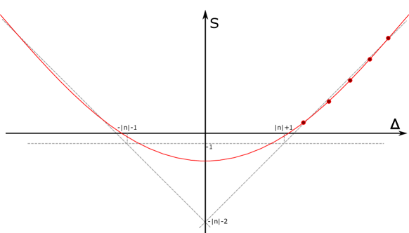
Figure 1: Trajectory of the length-2 operator for conformal spin $n=S_{2}$ as a function of the full dimension $\Delta$. The dots correspond to the physical operators with $S+n\in 2\mathbb{Z}_{\geq 0}$.

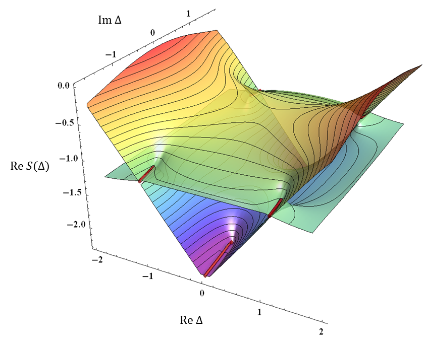
Figure 2: Riemann surface of the function $S(\Delta)$ for twist-2 operators.

Having these analytic properties in mind, we understand how to apply the QSC to the study of the BFKL spectrum: we need to analytically continue to non-integer spin $S$ and conformal spin $n$ not only the anomalous dimensions, but the QSC itself: Q-functions, their asymptotics and analytic structure etc. In the next section we are going to start from the brief description of the QSC basics. Then we will use this setup to consider the calculation of the LO BFKL kernel eigenvalue with non-zero conformal spin by the QSC method.

2.3 QSC approach to the BFKL spectrum of $\mathcal{N}=4$ SYM

We are going to present here the formulation of the QSC in terms of the Q-system and gluing conditions, the details of which can be found in Gromov:2014caa ; Gromov:2017blm ; Alfimov:2018cms . Algebraic part of the QSC framework is described as follows. For the $\mathcal{N}=4$ SYM we have the system of $2^{8}$ Q-functions, which are denoted as

$$Q_{a_{1},\ldots,a_{n}|i_{1},\ldots,i_{m}}(u)\;,\quad 1\leq n,m\leq 4.$$ (18)

The Q-functions (18) have two groups of indices: $a$’s are called “bosonic” and $i$’s are called “fermionic”. They are antisymmetric with respect to the exchange of any pair of indices in these two groups. Not all of the 256 Q-functions in question are independent. They are subject to the set of the so-called Plücker’s QQ-relations, which are written in Gromov:2014caa

$$Q_{A|I}Q_{Aab|I} = Q_{Aa|I}^{+}Q_{Ab|I}^{-}-Q_{Aa|I}^{-}Q_{Ab|I}^{+}\;,$$ (19)

$$Q_{A|I}Q_{A|Iij} = Q_{A|Ii}^{+}Q_{A|Ij}^{-}-Q_{Aa|Ii}^{-}Q_{Ab|Ij}^{+}\;,$$

$$Q_{Aa|I}Q_{A|Ii} = Q_{Aa|Ii}^{+}Q_{Ab|I}^{-}-Q_{Aa|Ii}^{-}Q_{A|I}^{+}\;,$$

where $A$ and $I$ are multi-indices from the set $\{1,2,3,4\}$.

The standard normalization is chosen to be

$$Q_{\emptyset|\emptyset}=1\;.$$ (20)

Then the structure of the QQ-relations allows to express the whole Q-system in terms of the “basic” set of $8$ Q-functions $Q_{a|\emptyset}$, $a=1,\ldots,4$ and $Q_{\emptyset|i}$, $i=1,\ldots,4$.

Let us now describe two symmetries of the Q-system, which respect the QQ-relations (19).

• Imposing the so-called unimodularity condition

  $$Q_{1234|1234}=1\;,$$ (21)

  we are able to introduce the system of Hodge-dual Q-functions

  $$Q^{a_{1}\ldots a_{n}|i_{1}\ldots i_{m}}\equiv(-1)^{nm}\epsilon^{b_{n+1}\ldots b_{4}a_{1}\ldots a_{n}}\epsilon^{j_{m+1}\ldots j_{4}i_{1}\ldots i_{m}}Q_{b_{n+1}\ldots b_{4}|j_{m+1}\ldots j_{4}}\;,$$ (22)

  where there is no summation over the repeated indices and which satisfy the same QQ-relations (19). The condition (21) allows to write down the following relations between the Q-functions with the lower and upper indices

  $$Q^{a|i}Q_{b|j}=-\delta^{i}_{j}\;, Q^{a|i}Q_{b|i}=-\delta^{a}_{b}\;,$$ (23)

  $$Q^{a|\emptyset}=(Q^{a|i})^{+}Q_{\emptyset|i}\;, Q^{\emptyset|i}=(Q^{a|i})^{+}Q_{a|\emptyset}\;,$$

  $$Q_{a|\emptyset}Q^{a|\emptyset}=0\;, Q_{\emptyset|i}Q^{\emptyset|i}=0\;.$$

• Another symmetry is called the H-symmetry. Its general form is given by

  $$Q_{A|I}\rightarrow\sum\limits_{|B|=|A|,|J|=|I|}(H_{b}^{[|A|-|I|]})_{A}^{B}(H_{f}^{[|A|-|I|]})_{I}^{J}Q_{B|J}\;,$$ (24)

  where the sum goes over the repeated multi-indices. The definition of $H_{I}^{J}$ is the following: $(H_{f})_{I}^{J}\equiv(H_{F}(u))_{i_{1}}^{j_{1}}(H_{F}(u))_{i_{2}}^{j_{2}}\ldots(H_{F}(u))_{i_{|I|}}^{j_{|I|}}$ and the same for $(H_{b})_{A}^{B}$ and $(H_{B}(u))_{a_{k}}^{b_{k}}$, $k=1,\ldots,|A|$ with $H_{B,F}(u)$ being $4\times 4$ $i$-periodic matrices. The unimodularity condition leads us to the restriction

  $$\det H_{B}(u)\det H_{F}(u)=1\;.$$ (25)

To proceed with the calculation of the spectrum of $\mathcal{N}=4$ SYM we have to endow the described Q-system with the analytic structure. To start with, we designate the basic Q-functions with this structure as ${\bf P}_{a}$ (same as $Q_{a|\emptyset}$), ${\bf P}^{a}$ ($Q^{a|\emptyset}$), ${\bf Q}_{i}$ ($Q_{\emptyset|i}$) and ${\bf Q}^{i}$ ($Q^{\emptyset|i}$). One can find the asymptotics of the Q-functions in Gromov:2017blm

$${\bf P}_{a}\simeq A_{a}u^{-\tilde{M}_{a}}\;,\quad{\bf P}^{a}\simeq A^{a}u^{\tilde{M}_{a}-1}\;,\quad{\bf Q}_{i}\simeq B_{i}u^{\hat{M}_{i}-1}\;,\quad{\bf Q}^{i}\simeq B^{i}u^{-\hat{M}_{i}}\;,$$ (26)

where $\tilde{M}_{a}$, $a=1,\ldots,4$ and $\hat{M}_{i}$, $i=1,\ldots,4$ are expressed in terms of Cartan charges of ${\rm PSU}(2,2|4)$ (i.e. quantum numbers of the states)

$$\tilde{M}_{a} = \left\{\frac{J_{1}+J_{2}-J_{3}}{2}+1,\frac{J_{1}-J_{2}+J_{3}}{2},\frac{-J_{1}+J_{2}+J_{3}}{2}+1,\frac{-J_{1}-J_{2}-J_{3}}{2}\right\},$$

$$\hat{M}_{i} = \left\{\frac{1}{2}\left(\Delta-S_{+}+2\right),\frac{1}{2}\left(\Delta+S_{+}\right),\frac{1}{2}\left(-\Delta-S_{-}+2\right),\frac{1}{2}\left(-\Delta+S_{-}\right)\right\}\;,$$ (27)

where $S_{\pm}=S_{1}\pm S_{2}$.

As the Q-system is generated by the set of $8$ basic Q-functions, we first ascribe them the analytic structure dictated by the classical limit of the Q-functions Gromov:2017blm . The minimal choice of the cut structure consistent with the asymptotics (26) is presented on the Figure 3.

Figure 3: Analytic structure of the ${\bf P}$- and ${\bf Q}$-functions on their defining sheet.

Then, according to the (19) we can generate two versions of the Q-system: upper half plane and lower half plane analytic (UHPA and LHPA respectively). In what follows we will define by $\mathcal{Q}_{a|i}$ the UHPA solution of the one of the QQ-relations from (19)

$$\mathcal{Q}_{a|i}^{+}-\mathcal{Q}_{a|i}^{-}={\bf P}_{a}{\bf Q}_{i}$$ (28)

with the large $u$ asymptotic

$$\mathcal{Q}_{a|i}\simeq-i\frac{A_{a}B_{i}}{-\tilde{M}_{a}+\hat{M}_{i}}u^{-\tilde{M}_{a}+\hat{M}_{i}}\;.$$ (29)

Substitution of the formulas ${\bf Q}_{i}=-\mathcal{Q}_{a|i}^{+}{\bf P}^{a}$ or ${\bf P}_{a}=-\mathcal{Q}_{a|i}{\bf Q}^{i}$ into (28) allows to fix the products of the coefficients of the leading asymptotics of the ${\bf P}$- and ${\bf Q}$-functions and for $a_{0},i_{0}=1,\ldots,4$ we get

$$A_{a_{0}}A^{a_{0}}=i\frac{\prod\limits_{j=1}^{4}\left(\tilde{M}_{a_{0}}-\hat{M}_{j}\right)}{\prod\limits_{\begin{subarray}{c}b=1\\ b\neq a_{0}\end{subarray}}\left(\tilde{M}_{a_{0}}-\tilde{M}_{b}\right)}\;,\quad B_{i_{0}}B^{i_{0}}=-i\frac{\prod\limits_{a=1}^{4}\left(\hat{M}_{i_{0}}-\tilde{M}_{a}\right)}{\prod\limits_{\begin{subarray}{c}j=1\\ j\neq i_{0}\end{subarray}}^{4}\left(\hat{M}_{i_{0}}-\hat{M}_{j}\right)}\;,$$ (30)

where there is no summation over the repeated indices $a_{0}$ and $i_{0}$.

An important consequence of the formula ${\bf Q}_{i}=-\mathcal{Q}_{a|i}{\bf P}^{a}$ combined with the formula (28) is the existence of a 4th order Baxter equation for the functions ${\bf Q}_{i}$, $i=1,\ldots,4$ (see Alfimov:2014bwa for the derivation)

$${\bf Q}_{i}^{[+4]} - {\bf Q}_{i}^{[+2]}\left[D_{1}-{\bf P}_{a}^{[+2]}{\bf P}^{a[+4]}D_{0}\right]+{\bf Q}_{i}\left[D_{2}-{\bf Q}_{a}{\bf P}^{a[+2]}D_{1}+{\bf P}_{a}{\bf P}^{a[+4]}D_{0}\right]-$$ (31)

$$- {\bf Q}_{i}^{[-2]}\left[\bar{D}_{1}+{\bf P}_{a}^{[-2]}{\bf P}^{a[-4]}\bar{D}_{0}\right]+{\bf Q}_{i}^{[-4]}=0\;,$$

where the functions $D_{0}$, $D_{1}$ and $D_{2}$ are given by

$$D_{0} = \left|\begin{array}[]{llll}{\bf P}^{1[+2]}&{\bf P}^{2[+2]}&{\bf P}^{3[+2]}&{\bf P}^{4[+2]}\\ {\bf P}^{1}&{\bf P}^{2}&{\bf P}^{3}&{\bf P}^{4}\\ {\bf P}^{1[-2]}&{\bf P}^{2[-2]}&{\bf P}^{3[-2]}&{\bf P}^{4[-2]}\\ {\bf P}^{1[-4]}&{\bf P}^{2[-4]}&{\bf P}^{3[-4]}&{\bf P}^{4[-4]}\end{array}\right|\;,\quad D_{1}=\left|(\begin{array}[]{llll}{\bf P}^{1[+4]}&{\bf P}^{2[+4]}&{\bf P}^{3[+4]}&{\bf P}^{4[+4]}\\ {\bf P}^{1}&{\bf P}^{2}&{\bf P}^{3}&{\bf P}^{4}\\ {\bf P}^{1[-2]}&{\bf P}^{2[-2]}&{\bf P}^{3[-2]}&{\bf P}^{4[-2]}\\ {\bf P}^{1[-4]}&{\bf P}^{2[-4]}&{\bf P}^{3[-4]}&{\bf P}^{4[-4]}\end{array}\right|,$$ (40)

$$D_{2} = \left|\begin{array}[]{llll}{\bf P}^{1[+4]}&{\bf P}^{2[+4]}&{\bf P}^{3[+4]}&{\bf P}^{4[+4]}\\ {\bf P}^{1[+2]}&{\bf P}^{2[+2]}&{\bf P}^{3[+2]}&{\bf P}^{4[+2]}\\ {\bf P}^{1[-2]}&{\bf P}^{2[-2]}&{\bf P}^{3[-2]}&{\bf P}^{4[-2]}\\ {\bf P}^{1[-4]}&{\bf P}^{2[-4]}&{\bf P}^{3[-4]}&{\bf P}^{4[-4]}\end{array}\right|\;,$$ (45)

while the bars over $\bar{D}_{1}$ and $\bar{D}_{2}$ are understood as the complex conjugation $\bar{f}(u)=\overline{f(\bar{u})}$ of the functions defined above. The same equation for ${\bf Q}^{i}$, $i=1,\ldots,4$ is valid, if we turn the functions ${\bf P}^{a}$ into ${\bf P}_{a}$ for $a=1,\ldots,4$.

One can see from (31) that if we are far away (high or low enough) from the real axis in the complex plane, the cut structures (see the Figure 3) of ${\bf P}$- and ${\bf Q}$-functions do not contradict each other. But as we approach the real axis, this is no longer the case and we have to cross the cut. This makes the QQ-relations ambiguous in the vicinity of the cuts, as the shifts by $\pm i/2$ may cross the cut and one may ask which contour to use to reach $u\pm i/2$ from the point $u$ or, in other words, which branch of the multi-valued function to use.

The way to resolve the analytic continuation ambiguity is to interpret the values of the ${\bf Q}$-function in the upper half plane, far enough from the cuts, as a ${\bf Q}$-function with the upper index ${\bf Q}^{i}$ and in the lower half plane the same ${\bf Q}$-function should obey the QQ-relations as if it was a function with lower index ${\bf Q}_{i}^{\uparrow}$. I.e. in the lower half plane this function satisfies (31), whereas in the upper half plane it satisfies the same equation with ${\bf P}_{a}$ interchanged with ${\bf P}^{a}$. The ${\uparrow}$ is added to indicate that ${\bf Q}_{i}^{{\uparrow}}$ does not have cuts in the lower half plane. To close the system of equations we notice that there is yet another way to build the set of functions ${\bf Q}_{i}^{{\uparrow}}$, satisfying (31) and having no cuts in the lower half plane. One can, starting from ${\bf Q}^{i}$, which has no cuts in the upper half plane and ${\bf P}^{a}$ – and build ${\bf Q}_{i}^{\downarrow}$ using QQ-relations. Then the complex conjugate of ${\bf Q}_{i}^{\downarrow}$ will satisfy (31) and will have no cuts in the lower half plane.

Indeed, due to the property, valid for real $S_{1}$, $S_{2}$ and $\Delta$ we can always assume that

$$\bar{{\bf P}}_{a}=C_{a}^{b}{\bf P}_{b}\;,\quad\bar{{\bf P}}^{a}=-C^{a}_{b}{\bf P}^{b}\;,\quad C=\textrm{diag}\{1,1,-1,-1\}$$ (46)

due to the H-symmetry. Thus if we complex conjugate the Baxter equation (31), we get the same equation for $\bar{{\bf Q}}_{j}$. This implies that ${\bf Q}_{i}^{\downarrow}(u)$ is a linear combination of $\bar{{\bf Q}}_{j}$ with regular coefficients

$${\bf Q}^{i}(u)=M^{ij}(u)\bar{{\bf Q}}_{j}(u)\;,\quad{\bf Q}_{i}(u)=\left(M^{-t}\right)_{ij}(u)\bar{{\bf Q}}^{j}(u)\;,$$ (47)

where $-t$ denotes the inversion and transposition of the matrix. Technically it will be more convenient to work with short cuts $[-2g,2g]$. We can connect the branch points of ${\bf Q}$ the way we like, but this would create an infinite ladder of cuts in the lower half plane. It will also modify the notion of the conjugate function, as the conjugation now will also involve the analytic continuation under the cut. So we conclude that in the short cut conventions the gluing condition reads as

$$\tilde{{\bf Q}}^{i}(u)=M^{ij}(u)\bar{{\bf Q}}_{j}(u)\;,\quad\tilde{{\bf Q}}_{i}(u)=\left(M^{-t}\right)_{ij}(u)\bar{{\bf Q}}^{j}(u)\;,$$ (48)

which we will use further. Let us now list the properties of $M^{ij}(u)$, which is called the gluing matrix. The details of the derivation of these properties can be found in Alfimov:2018cms . They are:

• $M^{ij}(u)$ is an $i$-periodic matrix of H-transformation.

• $M^{ij}(u)$ is analytic in the whole complex plane.

• $M^{ij}(u)$ is hermitian as a function

  $$\bar{M}^{ij}(u)=M^{ji}(u)\;.$$ (49)

There exist another additional symmetry of the ${\bf P}$-functions. The ${\bf P}$-functions of the states with the Cartan charges

$$\tilde{M}_{a} = \left\{2,1,0,-1\right\},$$ (50)

$$\hat{M}_{i} = \left\{\frac{1}{2}\left(\Delta-S_{+}+2\right)\;,\frac{1}{2}\left(\Delta+S_{+}\right)\;,\frac{1}{2}\left(-\Delta-S_{-}+2\right)\;,\frac{1}{2}\left(-\Delta+S_{-}\right)\right\}\;,$$

where $S_{\pm}\equiv S_{1}\pm S_{2}$, have the certain parity

$${\bf P}_{a}(-u)=(-1)^{a+1}{\bf P}_{a}(u)\;,\quad{\bf P}^{a}(-u)=(-1)^{a}{\bf P}^{a}(u)\;.$$ (51)

The conjugation symmetry and the symmetry above (51) lead to two additional constraints Alfimov:2018cms on the gluing matrix. Let us first concentrate on the physical states, when $S_{1}$ and $S_{2}$ are integer and have the same parity. As it follows from the power-like large $u$ asymptotics of the ${\bf Q}$-functions in this case, the only possible ansatz for the gluing matrix is a constant matrix. In Gromov:2014caa ; Alfimov:2018cms it was shown that for the physical length-2 states with the charges (50) from the abovementioned properties of the gluing matrix and two additional constraints mentioned earlier it follows that

$$M^{ij}\left(e^{i\pi\left(\hat{M}_{i}-\hat{M}_{j}\right)}+1\right)=0\;.$$ (52)

From (52), we immediately see that only when the difference between the charges is an odd integer, $M^{ij}$ is non-zero. It is the case only for

$$\hat{M}_{1}-\hat{M}_{2} = -S_{1}-S_{2}+1\;,$$ (53)

$$\hat{M}_{3}-\hat{M}_{4} = -S_{1}+S_{2}+1\;.$$

Therefore, taking into account the hermiticity of the gluing matrix, for integer $S_{1}$ and $S_{2}$, that have the same parity (i.e. for the physical states) the equations (52) lead to the gluing matrix

$$M^{ij}=\left(\begin{array}[]{cccc}0&M^{12}&0&0\\ \bar{M}^{12}&0&0&0\\ 0&0&0&M^{34}\\ 0&0&\bar{M}^{34}&0\end{array}\right)\;.$$ (54)

In the case of at least one of the spins $S_{1}$ and $S_{2}$ being non-integer, we see, that because all differences $\hat{M}_{i}-\hat{M}_{j}$ are non-integer the equations (52) can have only zero matrix as a solution, if this matrix is assumed to be constant. This leads us to the conclusion that the gluing matrix cannot be constant anymore for non-integer spins. The minimal way to do this keeping it $i$-periodic would be to add exponential contributions and get the following gluing matrix

$$M = \left(\begin{array}[]{cccc}M_{1}^{11}&M_{1}^{12}&M_{1}^{13}&M_{1}^{14}\\ \bar{M}_{1}^{12}&0&0&0\\ \bar{M}_{1}^{13}&0&M_{1}^{33}&M_{1}^{34}\\ \bar{M}_{1}^{14}&0&\bar{M}_{1}^{34}&M_{1}^{44}\\ \end{array}\right)+$$ (59)

$$+ \left(\begin{array}[]{cccc}0&0&M_{2}^{13}&M_{2}^{14}\\ 0&0&0&0\\ \bar{M}_{2}^{13}&0&0&0\\ \bar{M}_{2}^{14}&0&0&0\\ \end{array}\right)e^{2\pi u}+\left(\begin{array}[]{cccc}0&0&M_{3}^{13}&M_{3}^{14}\\ 0&0&0&0\\ \bar{M}_{3}^{13}&0&0&0\\ \bar{M}_{3}^{14}&0&0&0\\ \end{array}\right)e^{-2\pi u}\;.$$ (68)

To summarize, the key observation here is that if we want to consider non-physical states with $S_{1}$ or $S_{2}$ being non-integer, this inevitably requires modification of the gluing conditions. From now on let us use the notations for the spins coming from BFKL physics $S_{1}=S$ and $S_{2}=n$.

In the next Subsection we will briefly describe how the QQ-relations together with the gluing condition (48) can be used to compute numerically the function $S(\Delta,n)$.

2.4 Numerical solution

The QQ-system together with the gluing conditions allows for the efficient numerical algorithm, developed in Gromov:2015wca . This method was described in details with the Mathematica code attached in a recent review Gromov:2017blm . Here we describe the main steps very briefly.

First, one notices that the ${\bf P}_{a}$ and ${\bf P}^{a}$ functions, $a=1,\ldots,4$, which have only one short cut $[-2g,2g]$ on the main sheet of the Riemann surface, can be parametrized very efficiently as rapidly converging series expansions in powers of $1/x(u)$, where $x(u)=(u+\sqrt{u-2g}\sqrt{u+2g})/(2g)$. After that one can recover the whole Q-system in terms of these expansion coefficients. For that one first uses

$$\mathcal{Q}_{a|i}^{+}-\mathcal{Q}_{a|i}^{-}=-{\mathcal{Q}}_{b|i}^{+}{\bf P}_{a}{{\bf P}}^{b}\;,$$ (69)

which follows directly from (28) and ${\bf Q}_{i}=-\mathcal{Q}_{a|i}{\bf P}^{i}$, to solve for $\mathcal{Q}_{a|i}$. After that one finds ${\bf Q}_{i}$ and $\tilde{\bf Q}_{i}$ from

$${{\bf Q}}_{i}=-{\mathcal{Q}}_{a|i}^{+}{{\bf P}}^{a}\;\;,\;\;\tilde{{\bf Q}}_{i}=-{\mathcal{Q}}_{a|i}^{+}\tilde{{\bf P}}^{a}\;.$$ (70)

Note that this involves $\tilde{{\bf P}}^{a}$, which is the same series as ${{\bf P}}^{a}$, but with $x\to 1/x$ for $u\in[-2g,2g]$. In this way we reconstruct both ${\bf Q}_{i}$ and $\tilde{\bf Q}_{i}$ in terms of the expansion coefficients in ${\bf P}_{a}$ and ${\bf P}^{a}$. Finally, one fixes these coefficients from the gluing condition (48).

In practice for the numerical purposes one truncates the series expansion in ${\bf P}$. In this case the gluing condition cannot be satisfied exactly. The strategy is to minimize the discrepancy in the gluing condition by adjusting the coefficients numerically with a variation of a Newton method.

Application of the numerical procedure allows to calculate the dependence of the intercept function $j=S(\Delta=0,n=0)+2$ for zero conformal spin Gromov:2014bva on the ‘t Hooft coupling $\lambda$, which is drawn on the Figure 4. By fitting the polynomial dependence of this quantity on the coupling, we obtain several first coefficients

$$j(\lambda) = 1+0.07023049277268284\;\lambda-0.00337167607361\;\lambda^{2}$$

$$- 0.00064579607573\;\lambda^{3}+0.0002512619258\;\lambda^{4}+\mathcal{O}(\lambda^{5})\;.$$

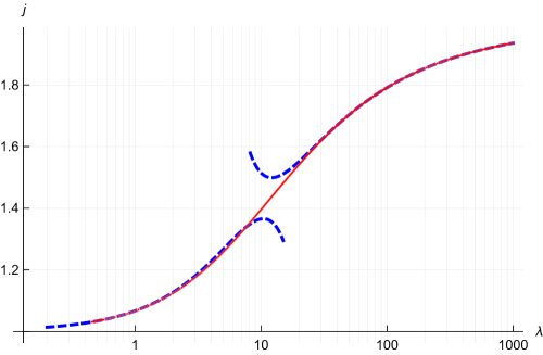
Figure 4: The dependence of the intercept function $j$ on the ‘t Hooft coupling $\lambda$ in the logarithmic scale. Data obtained from the numerical procedure are depicted in red. It represents a perfect interpolation between the weak Kotikov:2002ab ; Brower:2006ea and strong Costa:2012cb ; Kotikov:2013xu ; Brower:2013jga ; Gromov:2014bva coupling results (blue dashes).

Comparing the first two coefficients of (2.4), we find complete agreement with the LO (3) and NLO BFKL (2.1) kernel eigenvalues calculated at $\Delta=0$ and $n=0$.

Moreover, we can use our numerical algorithm to calculate not only the intercept functions, but also the BFKL kernel eigenvalues at different orders in $g$. Namely, in Gromov:2015vua from fitting the numerical values of the spin $S(\Delta,n)$ for $\Delta=0.45$ and $n=0$ for different values of the coupling constant one was able to extract the numerical values of the coefficients $\chi_{\textrm{N}^{k}\textrm{LO}}(\Delta=0.45)$ from (1), which are listed in the Table 1.

Table 1: Numerical values of the BFKL kernel eigenvalue at different orders.

Order	Value	Error
${\rm N^{2}LO}$	$10774.635818847176637957593127192456995929170948057653783424533229$	$10^{-61}$
${\rm N^{3}LO}$	$-366393.2052053917038937903507478544549935531959333919163403836$	$10^{-56}$
${\rm N^{4}LO}$	$1.332736355681126915694044310369828561521940588979476878854\times 10^{7}$	$10^{-51}$
${\rm N^{5}LO}$	$-4.921740136657916500913955552075070060721450958436559876\times 10^{8}$	$10^{-47}$

The first line of the Table 1 contains the numerical value of the NNLO BFKL kernel eigenvalue for $\Delta=0.45$, which was computed analytically for the first time in Gromov:2015vua by the QSC method. In that work there was shown that the calculated numerical value in the Table 1 coincides with the value of the analytic result for $\Delta=0.45$ with numerical accuracy $10^{-61}$.

In addition, the numerical algorithm can be used to explore the spectrum for non-zero values of conformal spin $n$ (to see the algorithm for different values of $\Delta$, $n$ and $g$ at work one can use the Mathematica file code_for_arxiv.nb from the Alfimov:2018cms arXiv submission). One can find the plots of the spin $S(0,n)$, which differs from the intercept function $j(n)$ by the additive constant $2$, for different (even non-integer) values of the conformal spin $n$ on the Figure 5.

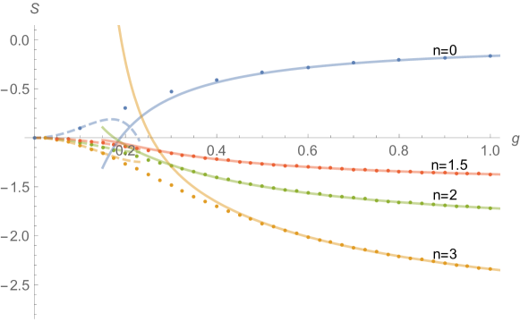
Figure 5: The dependence of the numerical values of the spin $S(0,n)$ on the coupling constant $g$, calculated for the conformal spins $n=0$, $n=3/2$, $n=2$ and $n=3$ (dots). The dashed lines represent weak coupling expansion and the continuous lines represent the strong coupling expansion of the spin obtained in Alfimov:2018cms .

To conclude, the numerical method of Gromov:2015wca allowed to obtain the BFKL kernel eigenvalue non-perturbatively with huge precision.

A number of analytic methods was developed to solve the QSC at small $g$ Marboe:2014gma ; Marboe:2014sya ; Gromov:2015vua ; Marboe:2017dmb ; Marboe:2018ugv . Unfortunately, those methods rely on a particular basis of $\eta$-functions, which works very well for the local operators of for BFKL eigenvalues at some integer values of $\Delta$, but are not sufficient in general. In the next section we will use an alternative method to obtain the LO BFKL kernel eigenvalue analytically. Recently, new very promising methods were developed in Lee:2017mhh ; Lee:2019bgq ; Lee:2019oml , based on the Mellin transformations, which could allow for a systematic analytic calculation of $S(\Delta)$ order by order in $g^{2}$ for generic $\Delta$.

2.5 Analytic results from QSC

Apart from the numerical results mentioned in the previous Section, a number of analytic results related to the BFKL spectrum was obtained recently using the QSC methods in Gromov:2014bva ; Alfimov:2014bwa ; Gromov:2015vua ; Gromov:2015dfa ; Gromov:2016rrp ; Alfimov:2018cms . To mention a few:

• NNLO BFKL kernel eigenvalue for the conformal spin $n=0$.

• Intercept function for arbitrary conformal spin $n$ up to NNLO order and partial result at NNNLO order.

• Strong coupling expansion of the intercept function for arbitrary value of the conformal spin $n$.

• Slope-to-slope function in the BPS point $\Delta=2$, $S=0$ and $n=0$ at all loops.

• Slope-to-intercept $dS(\Delta,n)/dn$ and curvature $d^{2}S(\Delta,n)/d\Delta^{2}$ functions in the BPS point $\Delta=0$, $S=-1$ and $n=1$ at all loops.

Here we demonstrate the power of the QSC method deriving the leading order Faddeev-Korchemsky Baxter equation with non-zero conformal spin for Lipatov spin chain analytically.

As explained above, we need to study the regime of the anomalous dimensions of the twist-2 operators, when the coupling constant $g^{2}\rightarrow 0$, such that $S\equiv S_{1}(\Delta,g)$ becomes $-1+{\cal O}(g^{2})$. According to the discussion in the previous section this is the case for $|\Delta|<1+|n|$. In other words one can say that we keep the ratio $\Lambda\equiv g^{2}/(S+1)$ finite, whereas the combination $w\equiv S+1={\cal O}(g^{2})$ can be used as a small expansion parameter. The second spin $S_{2}=n$ plays the role of a parameter.

In order to reproduce the Faddeev-Korchemsky Baxter equation we are going to utilise the subset of the QQ-relations known as ${\bf P}\mu$-system. The ${\bf P}\mu$-system is represented by the functions ${\bf P}_{a}(u)$, ${\bf P}^{a}(u)$, which we introduced before and of an anti-symmetric matrix $\mu_{ab}(u)$ (see Gromov:2013pga ; Gromov:2014caa for the detailed description). They satisfy the following equations

$$\tilde{\mu}_{ab}-\mu_{ab}={\bf P}_{a}\tilde{{\bf P}}_{b}-{\bf P}_{b}\tilde{{\bf P}}_{a}\;,\quad \tilde{{\bf P}}_{a}=\mu_{ab}{\bf P}^{b}\;,$$

$$\tilde{\mu}^{ab}-\mu^{ab}={\bf P}^{a}\tilde{{\bf P}}^{b}-{\bf P}^{b}\tilde{{\bf P}}^{a}\;,\quad \tilde{{\bf P}}^{a}=\mu^{ab}{\bf P}_{b}\;,$$

$${\bf P}_{a}{\bf P}^{a}=0\;,\quad\mu_{ab}\mu^{bc}=\delta_{a}^{c}\;,\quad \tilde{\mu}_{ab}=\mu_{ab}^{++}\;,\quad\tilde{\mu}^{ab}=\mu^{ab++}\;.$$

Before proceeding we remind a couple of notations. Our notation for the BFKL scaling parameter is $w=S+1$. It is also convenient to use the notation $\Lambda=g^{2}/w$.

To start solving the ${\bf P}\mu$-system in the BFKL regime we have to determine the scaling of the ${\bf P}$-, ${\bf Q}$- and $\mu$-functions in the small $w$ limit. In what follows we are going to use the arguments from Alfimov:2014bwa , thus as from (30) for the length-2 state in question (17) in the BFKL limit $A_{a}A^{a}=\mathcal{O}(w^{0})$ for $a=1,\ldots,4$ and $B_{i}B^{i}=\mathcal{O}(w^{0})$, these functions can be chosen to scale as $w^{0}$

$${\bf P}_{a}={\bf P}^{(0)}_{a}+\mathcal{O}(w)\;, {\bf P}^{a}={\bf P}^{(0)a}+\mathcal{O}(w)$$ (73)

$${\bf Q}_{i}={\bf Q}^{(0)}_{i}+\mathcal{O}(w)\;, {\bf Q}^{i}={\bf Q}^{(0)i}+\mathcal{O}(w)$$ (74)

and the $\mu$-functions scale as $w^{-2}$

$$\mu_{ab}=w^{-2}\left(\mu^{(0)}_{ab}+\mathcal{O}(w)\right)\;,\quad\mu^{ab}=w^{-2}\left(\mu^{(0)ab}+\mathcal{O}(w)\right)\;.$$ (75)

Additionally, as all the ${\bf P}$-functions for the length-2 states being considered possess the certain parity from the ${\bf P}\mu$-system equations (2.5) we can conclude that the functions $\mu_{ab}^{+}(u)$ have the certain parity.

Let us restrict ourselves from now on in this Section to the case of integer conformal spin $S_{2}=n$. We know that the ${\bf P}$-functions have only one cut on one of the sheets, therefore they can be written as a series in the Zhukovsky variable $x(u)=(u+\sqrt{u^{2}-4\Lambda w})/(2\sqrt{\Lambda w})$. Then, we are also allowed to apply the certain H-transformation to the ${\bf P}$-functions, which do not alter their asymptotics and parity. Applying this transformation, we can set the coefficients $A_{1}=A_{2}=-A^{3}=A^{4}=1$ and some other coeficients in the series in $x(u)$ to $0$. Thus, we arrive to the formulas in the LO

$${\bf P}^{(0)}_{1}=\frac{1}{u^{2}}\;,\quad{\bf P}^{(0)}_{2}=\frac{1}{u}\;, {\bf P}^{(0)}_{3}=A_{3}^{(0)}\;,\quad{\bf P}^{(0)}_{4}=A_{4}^{(0)}u+\frac{c_{4,1}^{(1)}}{\Lambda u}\;,$$ (76)

$${\bf P}^{(0)1}=A^{1(0)}u+\frac{c^{1,1(1)}}{\Lambda u}\;, {\bf P}^{(0)2}=A^{2(0)}\;,\quad{\bf P}^{(0)3}=-\frac{1}{u}\;,\quad{\bf P}^{(0)4}=\frac{1}{u^{2}}\;,$$

where

$$A_{3}^{(0)} = \frac{(\left(\Delta-n\right)^{2}-1)(\left(\Delta+n\right)^{2}-9)}{32i}\;,$$ (77)

$$A_{4}^{(0)} = \frac{(\left(\Delta+n\right)^{2}-1)(\left(\Delta-n\right)^{2}-25)}{96i}$$

originate from the expansion of (30) at small $w$ and $c_{4,1}^{(1)}$ and $c^{1,1(1)}$ are some yet unknown coefficients.

The situation with the asymptotics of the $\mu$-functions is more subtle. For non-zero $S$ it appears that the asymptotics of the $\mu$ cannot be power-like anymore Gromov:2014eha and the minimal modification of the leading asymptotics of the $\mu$-functions with the lower indices at $u\rightarrow\pm\infty$ is

$$\mu_{ab}\sim(u^{-S-1},u^{-S},u^{-S+1},u^{-S+1},u^{-S+2},u^{-S+3})e^{2\pi|u|}\;,$$ (78)

while the $\mu$-functions with the upper indices have the same asymptotics but in the reverse order. The fact that the asymptotics should be modified as (78) can be derived from the fact that the gluing matrix (59) asymptotic receives additional exponential terms. In the work Alfimov:2018cms it was shown, that the correct ansatz for the $\mu$-functions in the LO would be polynomials of the powers consistent with the asymptotics (78) for $S=-1+w$ and $w$ close to $0$. We do not write this ansatz explicitly as it is not important for further discussion.

Substituting (76) and the ansatz for the $\mu$-functions into (2.5) in the LO and from the analyticity properties of the ${\bf P}$- and $\mu$-functions we fix the constants $c^{1,1(1)}$ and $c_{4,1}^{(1)}$

$$c^{1,1(1)}=-c_{4,1}^{(1)}\;,\quad c_{4,1}^{(1)}=-\frac{i\Lambda}{96}\left(\left(\Delta^{2}-1\right)^{2}-2\left(\Delta^{2}+1\right)n^{2}+n^{4}\right)$$ (79)

and the $\mu$-functions in the LO up to an overall constant (we do not write them explicitly as they are not relevant for further discussion).

After the substitution of the LO ${\bf P}$-functions (76) together with (79) into (31) in the LO (for the same result with the zero conformal spin see Alfimov:2014bwa ), one can derive, that this 4th order Baxter equation factorizes

$$\left[(u+2i)^{2}D+(u-2i)^{2}D^{-1}\right. - \left.2u^{2}-\frac{17-(\Delta+n)^{2}}{4}\right]\times$$

$$\times \left[D+D^{-1}-2-\frac{1-(\Delta-n)^{2}}{4u^{2}}\right]{\bf Q}^{(0)}_{j}=0\;,$$

where $D=e^{i\partial_{u}}$ is the shift operator (the same equation with $n$ replaced by $-n$ is true for ${\bf Q}^{(0)j}$, $j=1,\ldots,4$). Thus, two out of four linearly independent solutions of the $4^{\rm th}$ order Baxter equation can be found by soliving the second order Baxter equation

$${\bf Q}^{(0)++}+{\bf Q}^{(0)--}+\left(-2+\frac{(\Delta-n)^{2}-1}{4u^{2}}\right){\bf Q}^{(0)}=0\;.$$ (81)

Redefining the Q-function to be $Q=\frac{{\bf Q}_{j}}{u^{2}}$ we exactly reproduce the Baxter equation for the $SL(2,\mathbb{C})$ spin chain Faddeev:1994zg ; DeVega:2001pu ; Derkachov:2001yn ; Derkachov:2002pb ; Derkachov:2002wz from the QSC for $\mathcal{N}=4$ SYM  which is a highly non-trivial test of the all-loop integrability of this theory. This derivation established the desired connection between the integrability in the 4D gauge theory in the BFKL limit and integrability of the $\mathcal{N}=4$ SYM. Having this result, one can go further and by using QSC explore many more quantities, such as NNLO BFKL kernel eigenvalue, numerical twist-2 and length-2 operator trajectories, intercept function, slope, curvature and slope-to-intercept function etc. (see Gromov:2015wca ; Gromov:2015vua ; Alfimov:2018cms and references therein).

3 Fishnet and BFKL

Above we described how the integrability, discovered in the BFKL regime of the QCD, can be understood as a part of a more general integrable structure of ${\cal N}=4$ SYM. In fact the data coming from the BFKL regime has played an essential role in fixing the dressing phase of the Beisert-Staudascher equations, which eventually resulted in our current understanding of integrability in this model.

Another extremely popular recent topic – Sachdev-Ye-Kitaev (SYK) model also has many similarities at the technical level with the problem of BFKL kernel diagonalization  Gross:2017hcz ; Klebanov:2016xxf ; Murugan:2017eto ; Kitaev (see also a recent review dedicated to this topic Rosenhaus:2019mfr ).

In this section, we will describe yet another example of CFT tightly related to the LO BFKL physics – the Fishnet CFT at any dimension (FCFT_D). We will explain its Feynman graph content (in planar approximation big graphs have the shape of regular square lattice – at the origin of the name “fishnet”) and reveal the origins of its integrbility, described in terms of the conformal $SO(1,D+1)$ spin chain. We will demonstrate how, in particular case of $D=2$ and zero conformal spin, the problem of computing the anomalous dimensions of the simplest operators, described by so-called wheel graphs, boils down to the calculation of the spectrum of Lipatov’s multi-reggeon Hamiltonian.

3.1 Fishnet integrable model

The $D-$dimensional fishnet biscalar conformal field theory (dubbed usually as fishnet CFT, or FCFT_D) is defined by the Lagrangian Kazakov:2018qez

$${\cal L}_{d}=N_{c}\,{\rm tr}[\bar{X}\,\,(-{\partial}_{\mu}{\partial}^{\mu})^{\frac{D}{4}-\omega}\,X+\bar{Z}\,\,(-{\partial}_{\mu}{\partial}^{\mu})^{\frac{D}{4}+\omega}\,Z+(4\pi)^{\frac{D}{2}}\xi^{2}\bar{X}\bar{Z}XZ]\;,$$ (82)

where $X,Z$ are complex $N_{c}\times N_{c}$ matrix fields and $\bar{X}\equiv X^{\dagger},\bar{Z}\equiv Z^{\dagger}$ are their Hermitian conjugates. The differential operator in an arbitrary power is defined in a standard way, as an integral operator. The action (82) should be supplemented with certain double-trace counterterms described in Fokken:2014soa ; Sieg:2016vap ; Grabner:2017pgm ; Gromov:2018hut (see also Kazakov:2018hrh and references therein).

The FCFT₄ case of the model (in $D=4$ dimensions), for the particular “isotropic” case $\omega=0$, has a local Lagrangian. It was proposed in Gurdogan:2015csr as a specific double scaling limit of the $\gamma$-deformed ${\cal N}=4$ SYM theory, combining strong (imaginary) deformation and weak coupling. The effective coupling constant is $\xi^{2}=g_{\rm YM}^{2}N_{c}e^{-i\gamma_{3}}/(4\pi)^{2}$, where the ‘t Hooft coupling $\lambda=g_{YM}^{2}N_{c}\rightarrow 0$ and the deformations parameter $\gamma_{3}\rightarrow i\infty$. In this limit, all the fields except for two scalars get decoupled leading to (82) with $D=4$ and $\omega=0$, but the model retains the $SU(N_{c})$ global symmetry, which is a remnant of the gauge symmetry of the original ${\cal N}=4$ SYM theory. In the planar limit $N_{c}\to\infty$, the FCFT is dominated by so-called fishnet Feynman graphs which have the structure of the regular square lattice. Such graphs appear to be integrable Zamolodchikov:1980mb ; Chicherin:2012yn ; Gromov:2017cja . For infinitely long operators at a critical coupling $\xi_{*}$ those graphs have a continuous limit which is believed to be described by a specific $O(2,4)$ 2D $\sigma$-model Basso:2018agi . At strong coupling $\xi\to\infty$ the ${\rm FQFT}_{4}$ has a classical description in terms of a dual string-bit fish-chain model as it was derived in Gromov:2019aku . This exact duality persists at the quantum level too Gromov:2019jfh .

The model has already a rich history of studying various physical quantities, such as explicit computations of spectra of local operators Gurdogan:2015csr ; Caetano:2016ydc and 4-point correlation functions Basso:2017jwq ; Derkachov:2018rot ; Grabner:2017pgm ; Gromov:2018hut . The QSC formalism, adopted for the $\gamma$-deformed ${\cal N}=4$ SYM theory Kazakov:2015efa , appeared in this limit particularly efficient for computations of anomalous dimensions of operators of the type ${\rm tr}Z^{L}(\bar{X}X)^{M}+{\rm permutations}$ and later was extended to a much wider class of operators in Gromov:2019jfh . The FCFT₄ also appears to possess a rich moduli space of flat vacua, which are quantum-mechanically stable in spite of the absence of supersymmetry in the model Karananas:2019fox (in the planar limit).

3.2 Spectrum of Fishnet model and LO BFKL

At the technical level there is a number of places where the study of the spectrum of the fishnet models goes along similar steps as the problem of the BFKL spectrum. The similarity of the integrable structure of both models is discussed below. Here we just consider a simple example of a dimension of operators of the type ${\rm tr}\Box^{n}Z^{2}X^{2}$ in $D=4,\;w=0$, where $\Box$ is the 4D Laplace operator. The dimensions $\Delta$ of these operators can be obtained by solving the equation Gromov:2018hut

$$\frac{1}{\xi^{4}}=\frac{\psi^{(1)}\left(\frac{1}{4}(4-\Delta)\right)-\psi^{(1)}\left(\frac{1}{4}(6-\Delta)\right)-\psi^{(1)}\left(\frac{\Delta}{4}\right)+\psi^{(1)}\left(\frac{1}{4}(2+\Delta)\right)}{(\Delta-2)}\;,$$ (83)

which is reminiscent of the LO BFKL eigenvalue (16), written in the form

$$\frac{1}{g^{2}}=\frac{4}{S+1}\left(-\psi\left(\frac{1+\Delta}{2}\right)-\psi\left(\frac{1-\Delta}{2}\right)+2\psi(1)\right)+\mathcal{O}\left(\frac{g^{2}}{S+1}\right)\;.$$ (84)

The derivation of E2 from a Baxter equation is also very similar, to what is described in the Section 2.5.

Whereas the above analogy is demonstrated only at the structural level, below we give a more precise relation between the BFKL Hamiltonian and the graph-building operator of the fishnet theory in $D=2$ and a particular, spin zero representation for physical spins.

3.3 Graph-building operator and BFKL kernel

We start from the case of general $D,w$. Suppose we want to compute the correlator of local operators ${\cal O}_{L}(z)={\rm tr}[Z(z)]^{L}$ in FCFT_D

$$K(z,y)=\langle{\cal O}_{L}(z)\,\,\bar{\cal O}_{L}(y)\rangle\;.$$ (85)

Due to the chiral property of the Lagrangian (82) the only planar Feynman graphs for this correlator have a “globe” configuration Figure 7, where “parallels” and “meridians” form a regular square-lattice everywhere except for the “south” and “north” poles. The edges are represented by the propagators in $D$ dimensions given by

$$G_{h}(x)=(x^{2})^{-\frac{D}{4}+\omega}\;,\quad G_{v}(x)=(x^{2})^{-\frac{D}{4}-\omega}$$ (86)

in horizontal and vertical directions respectively.

According to general properties of CFT, such correlator should have the form

$$K(z,y)={\rm const}\,\,|x-y|^{-2\Delta_{{\cal O}_{L}}}$$ (87)

where $\Delta$ is the conformal dimension of this operator.

To compute this correlator, it is worth considering a more general operator, of the type ${\cal O}(z_{1}\dots z_{L})={\rm tr}[Z(z_{1})\dots Z(z_{L})]$ and compute the correlation function

$$K(z_{1},\dots,z_{L}|y_{1},\dots,y_{L})=\langle{\cal O}(z_{1}\dots z_{L})\,\,\bar{\cal O}(y_{1}\dots y_{L})\rangle\;.$$ (88)

The planar Feynman graphs for such correlator are of cylindrical topology. One should open the ends of meridians converging on the “south” and “north” poles on the Figure 7). If we then amputate the propagators converging at the south pole we obtain the cylindrical configuration presented on the Figure 7. Such a graph can be represented at each order of perturbation theory as the corresponding power of the so-called graph-building operator, acting on the space $(\mathbb{R}^{D})^{\bigotimes L}$,

$$H^{(w)}_{L}(z_{1},z_{2},\dots,z_{L}|z_{1}^{\prime},z_{2}^{\prime},\dots,z_{L}^{\prime}) = G_{v}(x_{11^{\prime}})G_{v}(x_{22^{\prime}})\dots G_{v}(x_{22^{\prime}})\times$$ (89)

$$\times G_{h}(x_{1^{\prime}2^{\prime}})G_{h}(x_{2^{\prime}3^{\prime}})\dots G_{h}(x_{L^{\prime}1^{\prime}})\;,$$

where we use the notations $x_{ab}=x_{a}-x_{b}$. Then the above correlator (88) can be represented as Gurdogan:2015csr ; Gromov:2017blm

$$K(z_{1},\dots,z_{L}|y_{1},\dots,y_{L})=\langle z_{1}\dots z_{L}|\,\frac{1}{1-\xi^{2L}H^{(s)}_{L}}\,|y_{1}\dots y_{L}\rangle\;,$$ (90)

where the states $|y_{1}\dots y_{L}\rangle$ are taken in the usual coordinate representation. It is easy to see, already by power counting, or applying the inversion transformation, that each cylindrical graph entering the perturbative expansion in $\xi^{2}$ is conformal. Thus the whole correlator will have the coordinate dependence according to the Euclidean $D$-dimensional conformal symmetry corresponding to the $\mathfrak{so}(1,D+1)$ algebra.

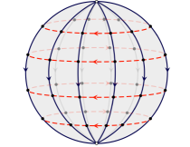
Figure 6: Planar Fishnet graphs of “globe” type arising in the computation of correlator (87). The edges belonging to red “parallels” and the black “meridians” correspond to propagators for two different scalar fields of the Lagrangian (82). Due to the chiral properties of vertices of this Lagrangian, no other planar diagrams in each loop order exist.

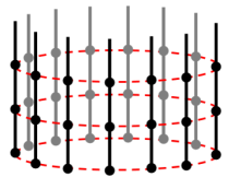
Figure 7: The cyllinder fishnet configuration resulting from the opening of the ends of propagators at the south and north poles of the globe (i.e. separating their coordinates) and amputating the propagators at the south pole. Such graphs can be computed by the Bethe-Salpeter procedure, using the integrability of the graph building operator, as described in this Section.

Introducing the 2D momenta conjugated to the coordinates $[p_{k},x_{k}]=i$, we can represent the operator (89) in a more compact form

$$H^{(s)}_{L} = (p^{2}_{1})^{-\frac{D}{4}+\omega}(x_{12})^{-\frac{D}{4}-\omega}(p^{2}_{2})^{-\frac{D}{4}+\omega}\times$$

$$\times (x_{23})^{-\frac{D}{4}-\omega}(p^{2}_{3})^{-\frac{D}{4}+\omega}\dots(p^{2}_{L})^{-\frac{D}{4}+\omega}(x_{L1})^{-\frac{D}{4}-\omega}\;.$$

The operator $H^{(w)}_{L}$ is known to be a conserved charge from the hierarchy of charges of the $so(1,D+1)$ spin chain encoded into the T-operator Zamolodchikov:1980mb ; Chicherin:2012yn ; Kazakov:2018hrh

$$T_{L}(u)={\rm Tr}_{\textrm{aux}}(\hat{R}^{1^{\prime}}_{1}(u)\hat{R}^{2^{\prime}}_{2}(u)\dots\hat{R}^{L^{\prime}}_{L}(u))$$ (92)

built from $L$ $R$-matrices acting in the product of principal series representations of $\mathfrak{so}(1,D+~{}1)$ with the weights $(\Delta_{1},0,0,\dots)\times(\Delta_{2},0,0,\dots)$

$$\hat{R}^{2^{\prime}}_{2}(u) = \langle x_{1}|R^{2^{\prime}}_{2}(u)|x_{1}^{\prime}\rangle=$$

$$= \frac{1}{(x_{12}^{2})^{-u-\frac{D}{2}+\Delta_{+}}(x_{21^{\prime}}^{2})^{u+\frac{D}{2}+\Delta_{-}}(x_{1^{\prime}2^{\prime}}^{2})^{-u+\frac{D}{2}-\Delta_{+}}(x_{12^{\prime}}^{2})^{u+\frac{D}{2}-\Delta_{-}}}\;,$$

where $\Delta_{\pm}=\frac{\Delta_{1}\pm\Delta_{2}}{2}$. The matrix multiplication in auxiliary space in (92) is understood as the integration $\int d^{2}z\langle x|\dots|z\rangle\langle z|\dots|y\rangle$ and the trace ${\rm Tr}_{\textrm{aux}}$ is understood as ${\rm Tr}_{\textrm{aux}}(\dots)=\int d^{2}z\langle z|\dots|z\rangle$.

We can also use the momenta $p_{j}$ to represent the $R$-matrix in the form

$$R_{ab}(u,\xi)=(x^{2}_{ab})^{u+\frac{D}{2}-\Delta_{+}}(p^{2}_{a})^{u+\Delta_{-}}(p^{2}_{b})^{u-\Delta_{-}}(x_{ab}^{2})^{u-\frac{D}{2}+\Delta_{+}}\;.$$ (94)

Indeed, if we take $u=-\frac{D}{2}+\Delta_{+}+\epsilon$ and $\Delta_{+}=\frac{D}{4}$, then the first factor in (3.3) in the limit $\epsilon\to 0$ disappears and the last one effectively becomes $\frac{1}{(x_{1^{\prime}2^{\prime}})^{\frac{D}{2}}}\sim\epsilon^{-1}\delta^{(D)}(x_{1^{\prime}2^{\prime}})$, and it is easy to see that

$$T_{L}(u)\sim\frac{1}{\epsilon^{L}}H_{L}^{(w)},\quad\text{where}\quad\Delta_{1}=\frac{D}{4}-w,\quad\Delta_{2}=\frac{D}{4}+w\;.$$ (95)

An interesting particular case of (92), mentioned in Chicherin:2012yn is the limit $u\to 0$, when $\Delta_{1}=\Delta_{2}\equiv\Delta$, since it is the only way to generate from it the local conserved charge – the spin chain hamiltonian with nearest neighbours interaction. Indeed, the $R$-matrix becomes in this limit

$$R_{ab}(u,\xi)=1+uh_{ab}+{\cal O}(u^{2})\;,$$ (96)

where

$$h_{ab}(\Delta) = 2\log(x^{2}_{ab})+(x_{ab}^{2})^{\frac{D}{2}-\Delta}\log(p^{2}_{a}p^{2}_{b})(x_{ab}^{2})^{-\frac{D}{2}+\Delta}=$$

$$= (p_{a}^{2})^{-\frac{D}{2}+\Delta}\log(x^{2}_{ab})(p_{a}^{2})^{\frac{D}{2}-\Delta}+(p_{b}^{2})^{-\frac{D}{2}+\Delta}\log(x^{2}_{ab})(p_{b}^{2})^{\frac{D}{2}-\Delta}+\log(p^{2}_{a}p^{2}_{b})\;,$$

which gives the Heisenberg hamiltonian for non-compact $SO(1,D+1)$ spin chain with nearest neighbors interaction of spins (with conformal spin $\Delta$):

$${\cal H}_{\Delta}=\sum_{a=1}^{L}\,h_{ab}(\Delta)\;,$$ (98)

For the particular dimension $D=2$ and conformal spin $\Delta=0$, we obtain from here the famous Lipatov’s $SL(2,\mathbb{C})$ spin chain describing the BFKL physics of interacting reggeized gluons in LO approximation Lipatov:1993yb

$$h_{ab}^{BFKL}=2\log(x^{2}_{ab})+(x_{ab}^{2})\log(p^{2}_{a}p^{2}_{b})(x_{ab}^{2})^{-1}\;.$$ (99)

In the particular case of two interacting reggeized gluons (Pomeron state) the spin chain reduces to two-spin hamiltonian

$${\cal H}_{\Delta}=2h_{12}^{BFKL}$$ (100)

with the spectrum given by the RHS of (84).

In this way, we see that the BFKL physics in LO approximation emerges as a particular case of $D$-dimensional Fishnet CFT, as it was first noticed in Kazakov:2018qez .

4 Conclusions

In this short review we made an attempt to briefly explain the studies of the BFKL spectrum in $\mathcal{N}=4$ SYM, which were inspired by the works of Lev Lipatov on the BFKL integrability in the 4D gauge theories without and with supersymmetry. His ideas have led to a very significant progress in understanding the BFKL spectrum of $\mathcal{N}=4$ SYM, where it was possible to build the bridge between the integrability of $\mathcal{N}=4$ SYM and integrability of the BFKL limit in the gauge theory. The usage of the Quantum Spectral Curve method in this limit has led to a series of new analytic and numerical results mentioned in this review.

The key feature utilized to link the results (including BFKL spectrum) in $\mathcal{N}=4$ SYM and QCD is the Kotikov-Lipatov’s principle of maximal transcendentality Kotikov:2000pm ; Kotikov:2001sc . In the Section 2.1 we illustrated this principle with an example of the NLO BFKL kernel eigenvalue in $\mathcal{N}=4$ SYM and QCD. In general, this principle goes much beyond the BFKL spectrum. Many more observables in $\mathcal{N}=4$ SYM admit this principle and reproduce the most transcendental part of the corresponding results in QCD. Another key observation by Lipatov Kotikov:2000pm , which allowed to connect the integrability of $\mathcal{N}=4$ SYM with the BFKL regime, is the relation between the BFKL regime and the dimensions of the operators in $\mathcal{N}=4$ SYM explained in the Section 2.2. This enabled the QSC method to be applied for the BFKL spectrum.

We also described here another special limit of $\mathcal{N}=4$ SYM similar in spirit to the BFKL limit, leading to the Fishnet CFT, currently actively studied in the literature. We explained here the generalization of the Fishnet CFT from four to any number $D$ of dimensions. It appears that, at $D=2$ and a special value of spin of the involved fields, the Fishnet CFT reduces to Lipatov’s integrable spin chain describing the interacting reggeized gluons in LO BFKL approximation of QCD. This remarkable correspondence can open new ways for the study of BFKL physics.

A great deal of the work presented here has been inspired by the ideas of Lev Lipatov. These ideas continue to influence a large community of theoretical physicists working on various non-perturbative aspects of quantum gauge theories. They find applications in a variety of domains of theoretical physics, including the integrable field theories. The BFKL spectrum of $\mathcal{N}=4$ SYM is only one of many such applications, where Lev Lipatov’s ideas gave rise to a great progress and revealed new intriguing problems, which still wait for their solution.

All three of us had the privilege to know Lev Lipatov personally and had the chance to appreciate, in numerous conversations, his outstanding personality and enormous talent. For one of us (V.K.), Lev Lipatov has been a dear friend over many years. For another (N.G.), Lev Nikolaevich was a dedicated and caring teacher who, over many years, greatly shaped his taste in research and was always available with deep insight and advice. And for the latter of us (M.A.), Lev Lipatov, despite being personally acquainted with him for a short time, left a great heritage of inspiring ideas and will always be an outstanding researcher to look up to.

For us, he will always be a great example of selfless devotion to science.

Acknowledgements

M.A. is grateful to Masha N. for her kind support during the work on this text. The work of N.G. was supported by the ERC grant 865075 EXACTC.

References

- (1) E. A. Kuraev, L. N. Lipatov and V. S. Fadin, The Pomeranchuk Singularity in Nonabelian Gauge Theories, Sov. Phys. JETP 45 (1977) 199.
- (2) I. I. Balitsky and L. N. Lipatov, The Pomeranchuk Singularity in Quantum Chromodynamics, Sov. J. Nucl. Phys. 28 (1978) 822.
- (3) L. Lipatov, The Bare Pomeron in Quantum Chromodynamics, Sov.Phys.JETP 63 (1986) 904.
- (4) V. S. Fadin and L. Lipatov, BFKL pomeron in the next-to-leading approximation, Phys.Lett. B429 (1998) 127 [hep-ph/9802290].
- (5) L. N. Lipatov, Asymptotic behavior of multicolor QCD at high energies in connection with exactly solvable spin models, JETP Lett. 59 (1994) 596 [hep-th/9311037].
- (6) L. N. Lipatov, High-energy asymptotics of multicolor QCD and two-dimensional conformal field theories, Phys. Lett. B309 (1993) 394.
- (7) L. D. Faddeev and G. P. Korchemsky, High-energy QCD as a completely integrable model, Phys. Lett. B342 (1995) 311 [hep-th/9404173].
- (8) S. E. Derkachov, G. Korchemsky and A. Manashov, Noncompact Heisenberg spin magnets from high-energy QCD: 1. Baxter Q operator and separation of variables, Nucl.Phys. B617 (2001) 375 [hep-th/0107193].
- (9) H. De Vega and L. Lipatov, Interaction of reggeized gluons in the Baxter-Sklyanin representation, Phys.Rev. D64 (2001) 114019 [hep-ph/0107225].
- (10) S. E. Derkachov, G. Korchemsky, J. Kotanski and A. Manashov, Noncompact Heisenberg spin magnets from high-energy QCD. 2. Quantization conditions and energy spectrum, Nucl.Phys. B645 (2002) 237 [hep-th/0204124].
- (11) S. E. Derkachov, G. Korchemsky and A. Manashov, Noncompact Heisenberg spin magnets from high-energy QCD. 3. Quasiclassical approach, Nucl.Phys. B661 (2003) 533 [hep-th/0212169].
- (12) A. Kotikov and L. Lipatov, NLO corrections to the BFKL equation in QCD and in supersymmetric gauge theories, Nucl.Phys. B582 (2000) 19 [hep-ph/0004008].
- (13) A. Kotikov and L. Lipatov, DGLAP and BFKL equations in the N=4 supersymmetric gauge theory, Nucl.Phys. B661 (2003) 19 [hep-ph/0208220].
- (14) A. V. Kotikov, L. N. Lipatov, A. Rej, M. Staudacher and V. N. Velizhanin, Dressing and Wrapping, J. Stat. Mech. 0710 (2007) P10003 [0704.3586].
- (15) J. A. Minahan and K. Zarembo, The Bethe-ansatz for N = 4 super Yang-Mills, JHEP 03 (2003) 013 [hep-th/0212208].
- (16) L. N. Lipatov, Evolution equations in QCD, in Perspectives in hadronic physics. Proceedings, Conference, Trieste, Italy, May 12-16, 1997, pp. 413–427, 1997.
- (17) L. N. Lipatov, Next-to-leading corrections to the BFKL equation and the effective action for high energy processes in QCD, Nucl. Phys. Proc. Suppl. 99A (2001) 175.
- (18) N. Beisert, C. Kristjansen and M. Staudacher, The Dilatation operator of conformal N=4 superYang-Mills theory, Nucl. Phys. B664 (2003) 131 [hep-th/0303060].
- (19) I. Bena, J. Polchinski and R. Roiban, Hidden symmetries of the AdS(5) x S**5 superstring, Phys. Rev. D69 (2004) 046002 [hep-th/0305116].
- (20) V. A. Kazakov, A. Marshakov, J. A. Minahan and K. Zarembo, Classical/quantum integrability in AdS/CFT, JHEP 05 (2004) 024 [hep-th/0402207].
- (21) N. Beisert, V. A. Kazakov, K. Sakai and K. Zarembo, The Algebraic curve of classical superstrings on AdS(5) x S**5, Commun. Math. Phys. 263 (2006) 659 [hep-th/0502226].
- (22) R. A. Janik, The AdS(5) x S**5 superstring worldsheet S-matrix and crossing symmetry, Phys. Rev. D73 (2006) 086006 [hep-th/0603038].
- (23) N. Beisert and R. Roiban, Beauty and the twist: The Bethe ansatz for twisted N=4 SYM, JHEP 08 (2005) 039 [hep-th/0505187].
- (24) N. Beisert, B. Eden and M. Staudacher, Transcendentality and Crossing, J.Stat.Mech. 0701 (2007) P01021 [hep-th/0610251].
- (25) J. Ambjorn, R. A. Janik and C. Kristjansen, Wrapping interactions and a new source of corrections to the spin-chain/string duality, Nucl. Phys. B736 (2006) 288 [hep-th/0510171].
- (26) N. Gromov, V. Kazakov, A. Kozak and P. Vieira, Exact Spectrum of Anomalous Dimensions of Planar N = 4 Supersymmetric Yang-Mills Theory: TBA and excited states, Lett. Math. Phys. 91 (2010) 265 [0902.4458].
- (27) D. Bombardelli, D. Fioravanti and R. Tateo, Thermodynamic Bethe Ansatz for planar AdS/CFT: A Proposal, J. Phys. A42 (2009) 375401 [0902.3930].
- (28) N. Gromov, V. Kazakov and P. Vieira, Exact Spectrum of Anomalous Dimensions of Planar N=4 Supersymmetric Yang-Mills Theory, Phys. Rev. Lett. 103 (2009) 131601 [0901.3753].
- (29) G. Arutyunov and S. Frolov, Thermodynamic Bethe Ansatz for the AdS(5) x S(5) Mirror Model, JHEP 05 (2009) 068 [0903.0141].
- (30) N. Gromov, V. Kazakov, S. Leurent and D. Volin, Quantum spectral curve for arbitrary state/operator in AdS5/CFT4, JHEP 09 (2015) 187 [1405.4857].
- (31) N. Gromov and F. Levkovich-Maslyuk, Quantum Spectral Curve for a cusped Wilson line in SYM, JHEP 04 (2016) 134 [1510.02098].
- (32) N. Gromov, Introduction to the Spectrum of SYM and the Quantum Spectral Curve, 1708.03648.
- (33) V. Kazakov, Quantum Spectral Curve of -twisted SYM theory and fishnet CFT, 1802.02160.
- (34) N. Gromov, F. Levkovich-Maslyuk and G. Sizov, Quantum Spectral Curve and the Numerical Solution of the Spectral Problem in AdS5/CFT4, JHEP 06 (2016) 036 [1504.06640].
- (35) M. Alfimov, N. Gromov and V. Kazakov, QCD Pomeron from AdS/CFT Quantum Spectral Curve, JHEP 07 (2015) 164 [1408.2530].
- (36) N. Gromov, F. Levkovich-Maslyuk and G. Sizov, Pomeron Eigenvalue at Three Loops in 4 Supersymmetric Yang-Mills Theory, Phys. Rev. Lett. 115 (2015) 251601 [1507.04010].
- (37) S. Caron-Huot and M. Herranen, High-energy evolution to three loops, JHEP 02 (2018) 058 [1604.07417].
- (38) M. Alfimov, N. Gromov and G. Sizov, BFKL spectrum of = 4: non-zero conformal spin, JHEP 07 (2018) 181 [1802.06908].
- (39) O. Gurdogan and V. Kazakov, New Integrable 4D Quantum Field Theories from Strongly Deformed Planar 4 Supersymmetric Yang-Mills Theory, Phys. Rev. Lett. 117 (2016) 201602 [1512.06704].
- (40) J. Caetano, O. Gurdogan and V. Kazakov, Chiral limit of = 4 SYM and ABJM and integrable Feynman graphs, JHEP 03 (2018) 077 [1612.05895].
- (41) D. Chicherin, V. Kazakov, F. Loebbert, D. Müller and D.-l. Zhong, Yangian Symmetry for Bi-Scalar Loop Amplitudes, JHEP 05 (2018) 003 [1704.01967].
- (42) N. Gromov, V. Kazakov, G. Korchemsky, S. Negro and G. Sizov, Integrability of Conformal Fishnet Theory, JHEP 01 (2018) 095 [1706.04167].
- (43) D. Chicherin, V. Kazakov, F. Loebbert, D. Müller and D.-l. Zhong, Yangian Symmetry for Fishnet Feynman Graphs, Phys. Rev. D96 (2017) 121901 [1708.00007].
- (44) D. Grabner, N. Gromov, V. Kazakov and G. Korchemsky, Strongly -Deformed Supersymmetric Yang-Mills Theory as an Integrable Conformal Field Theory, Phys. Rev. Lett. 120 (2018) 111601 [1711.04786].
- (45) O. Mamroud and G. Torrents, RG stability of integrable fishnet models, JHEP 06 (2017) 012 [1703.04152].
- (46) V. Kazakov and E. Olivucci, Biscalar Integrable Conformal Field Theories in Any Dimension, Phys. Rev. Lett. 121 (2018) 131601 [1801.09844].
- (47) G. K. Karananas, V. Kazakov and M. Shaposhnikov, Spontaneous Conformal Symmetry Breaking in Fishnet CFT, 1908.04302.
- (48) N. Gromov, V. Kazakov and G. Korchemsky, Exact Correlation Functions in Conformal Fishnet Theory, JHEP 08 (2019) 123 [1808.02688].
- (49) S. Derkachov, V. Kazakov and E. Olivucci, Basso-Dixon Correlators in Two-Dimensional Fishnet CFT, JHEP 04 (2019) 032 [1811.10623].
- (50) V. Kazakov, E. Olivucci and M. Preti, Generalized fishnets and exact four-point correlators in chiral CFT4, JHEP 06 (2019) 078 [1901.00011].
- (51) B. Basso, J. Caetano and T. Fleury, Hexagons and Correlators in the Fishnet Theory, JHEP 11 (2019) 172 [1812.09794].
- (52) G. P. Korchemsky, Exact scattering amplitudes in conformal fishnet theory, JHEP 08 (2019) 028 [1812.06997].
- (53) S. Dutta Chowdhury, P. Haldar and K. Sen, On the Regge limit of Fishnet correlators, JHEP 10 (2019) 249 [1908.01123].
- (54) N. Gromov and A. Sever, The Holographic Dual of Strongly -deformed N=4 SYM Theory: Derivation, Generalization, Integrability and Discrete Reparametrization Symmetry, 1908.10379.
- (55) B. Basso, G. Ferrando, V. Kazakov and D.-l. Zhong, Thermodynamic Bethe Ansatz for Fishnet CFT, 1911.10213.
- (56) S. Derkachov and E. Olivucci, Exactly solvable magnet of conformal spins in four dimensions, 1912.07588.
- (57) T. Adamo and S. Jaitly, Twistor fishnets, J. Phys. A53 (2020) 055401 [1908.11220].
- (58) R. de Mello Koch, W. LiMing, H. J. R. Van Zyl and J. P. Rodrigues, Chaos in the Fishnet, Phys. Lett. B793 (2019) 169 [1902.06409].
- (59) A. V. Kotikov and A. I. Onishchenko, Dglap and bfkl equations in sym: from weak to strong coupling, 1908.05113.
- (60) M. S. Costa, V. Goncalves and J. Penedones, Conformal Regge theory, JHEP 1212 (2012) 091 [1209.4355].
- (61) A. V. Kotikov, L. N. Lipatov and V. N. Velizhanin, Anomalous dimensions of Wilson operators in N=4 SYM theory, Phys. Lett. B557 (2003) 114 [hep-ph/0301021].
- (62) N. Gromov, V. Kazakov, S. Leurent and D. Volin, Quantum spectral curve for , Phys.Rev.Lett. 112 (2014) 011602 [1305.1939].
- (63) C. Marboe and D. Volin, Quantum spectral curve as a tool for a perturbative quantum field theory, Nucl. Phys. B899 (2015) 810 [1411.4758].
- (64) C. Marboe, V. Velizhanin and D. Volin, Six-loop anomalous dimension of twist-two operators in planar SYM theory, JHEP 07 (2015) 084 [1412.4762].
- (65) C. Marboe and V. Velizhanin, Twist-2 at seven loops in planar = 4 SYM theory: full result and analytic properties, JHEP 11 (2016) 013 [1607.06047].
- (66) C. Marboe and D. Volin, The full spectrum of AdS5/CFT4 I: Representation theory and one-loop Q-system, J. Phys. A51 (2018) 165401 [1701.03704].
- (67) C. Marboe and D. Volin, The full spectrum of AdS5/CFT4 II: Weak coupling expansion via the quantum spectral curve, 1812.09238.
- (68) N. Gromov and V. Kazakov, Analytic continuation in spin of the baxter equation solutions for twist-2 operators, unpublished (2013) .
- (69) R. A. Janik, Twist-two operators and the BFKL regime - nonstandard solutions of the Baxter equation, JHEP 1311 (2013) 153 [1309.2844].
- (70) A. V. Kotikov and V. N. Velizhanin, Analytic continuation of the Mellin moments of deep inelastic structure functions, hep-ph/0501274.
- (71) R. C. Brower, J. Polchinski, M. J. Strassler and C.-I. Tan, The Pomeron and gauge/string duality, JHEP 0712 (2007) 005 [hep-th/0603115].
- (72) M. S. Costa, J. Drummond, V. Goncalves and J. Penedones, The role of leading twist operators in the Regge and Lorentzian OPE limits, JHEP 1404 (2014) 094 [1311.4886].
- (73) R. C. Brower, M. Costa, M. Djuric, T. Raben and C.-I. Tan, Conformal Pomeron and Odderon in Strong Coupling, in International Workshop on Low X Physics (Israel 2013) Eilat, Israel, May 30-June 04, 2013, 2013, 1312.1419, http://inspirehep.net/record/1267665/files/arXiv:1312.1419.pdf.
- (74) N. Gromov, F. Levkovich-Maslyuk, G. Sizov and S. Valatka, Quantum spectral curve at work: from small spin to strong coupling in = 4 SYM, JHEP 07 (2014) 156 [1402.0871].
- (75) A. V. Kotikov and L. N. Lipatov, Pomeron in the N=4 supersymmetric gauge model at strong couplings, Nucl. Phys. B874 (2013) 889 [1301.0882].
- (76) R. N. Lee and A. I. Onishchenko, ABJM quantum spectral curve and Mellin transform, JHEP 05 (2018) 179 [1712.00412].
- (77) R. N. Lee and A. I. Onishchenko, Toward an analytic perturbative solution for the ABJM quantum spectral curve, 1807.06267.
- (78) R. N. Lee and A. I. Onishchenko, ABJM quantum spectral curve at twist 1: algorithmic perturbative solution, JHEP 11 (2019) 018 [1905.03116].
- (79) N. Gromov and F. Levkovich-Maslyuk, Quark-anti-quark potential in 4 SYM, JHEP 12 (2016) 122 [1601.05679].
- (80) N. Gromov and G. Sizov, Exact Slope and Interpolating Functions in N=6 Supersymmetric Chern-Simons Theory, Phys. Rev. Lett. 113 (2014) 121601 [1403.1894].
- (81) D. J. Gross and V. Rosenhaus, The Bulk Dual of SYK: Cubic Couplings, JHEP 05 (2017) 092 [1702.08016].
- (82) I. R. Klebanov and G. Tarnopolsky, Uncolored random tensors, melon diagrams, and the Sachdev-Ye-Kitaev models, Phys. Rev. D95 (2017) 046004 [1611.08915].
- (83) J. Murugan, D. Stanford and E. Witten, More on Supersymmetric and 2d Analogs of the SYK Model, JHEP 08 (2017) 146 [1706.05362].
- (84) A. Kitaev, “A simple model of quantum holography.” Talks at KITP http://online.kitp.ucsb.edu/online/entangled15/kitaev/ and http://online.kitp.ucsb.edu/online/entangled15/kitaev2/, April and May, 2015.
- (85) V. Rosenhaus, An introduction to the SYK model, 1807.03334.
- (86) J. Fokken, C. Sieg and M. Wilhelm, A piece of cake: the ground-state energies in -deformed = 4 SYM theory at leading wrapping order, JHEP 09 (2014) 078 [1405.6712].
- (87) C. Sieg and M. Wilhelm, On a CFT limit of planar -deformed SYM theory, Phys. Lett. B756 (2016) 118 [1602.05817].
- (88) A. B. Zamolodchikov, ’FISHNET’ DIAGRAMS AS A COMPLETELY INTEGRABLE SYSTEM, Phys. Lett. 97B (1980) 63.
- (89) D. Chicherin, S. Derkachov and A. P. Isaev, Conformal group: R-matrix and star-triangle relation, JHEP 04 (2013) 020 [1206.4150].
- (90) B. Basso and D.-l. Zhong, Continuum limit of fishnet graphs and AdS sigma model, JHEP 01 (2019) 002 [1806.04105].
- (91) N. Gromov and A. Sever, Derivation of the Holographic Dual of a Planar Conformal Field Theory in 4D, Phys. Rev. Lett. 123 (2019) 081602 [1903.10508].
- (92) B. Basso and L. J. Dixon, Gluing Ladder Feynman Diagrams into Fishnets, Phys. Rev. Lett. 119 (2017) 071601 [1705.03545].
- (93) V. Kazakov, S. Leurent and D. Volin, T-system on T-hook: Grassmannian Solution and Twisted Quantum Spectral Curve, JHEP 12 (2016) 044 [1510.02100].
- (94) V. K. David Grabner, Nikolay Gromov and G. Korchemsky, in preparation , .
- (95) A. V. Kotikov and L. N. Lipatov, DGLAP and BFKL evolution equations in the N=4 supersymmetric gauge theory, in 35th Annual Winter School on Nuclear and Particle Physics Repino, Russia, February 19-25, 2001, 2001, hep-ph/0112346, http://alice.cern.ch/format/showfull?sysnb=2289957.