The composite X-ray spectrum of 3CRR Quasars

Abstract

The reason for the difference in the composite X-ray spectrum between radio-loud quasars (RLQs) and radio-quiet quasars (RQQs) is still unclear. To study this difference, we built a new composite X-ray spectrum of RLQs by using Chandra X-ray data and Sloan Digital Sky Survey (SDSS) optical data for the sample of 3CRR quasars. We find the X-ray spectra of all 3CRR quasars except for 3C 351 have no soft X-ray excess and can be fitted with an absorbed power-law model well. Our composite X-ray spectrum is similar to that of Shang et al. (2011) for RLQs, showing higher hard X-ray and lower soft X-ray flux than the composite X-ray spectrum of RQQs. Most blazar-like 3CRR quasars have higher X-ray flux than the median composite X-ray spectrum, which could be related to the contribution of beamed jet emission at X-ray band. From the literature, we find that nineteen 3CRR quasars have extended X-ray emission related to radio jets, indicating inevitable contribution of jets at X-ray band. In contrast to RQQs, the X-ray photon index of 3CRR quasars does not correlate with the Eddington ratio. Our results suggest that the jet emission at X-ray band in RLQs could be related with the difference of composite X-ray spectrum between RLQs and RQQs.

1 Introduction

X-ray emission appears to be nearly universal from active galactic nuclei (AGNs) and is often used to detect AGNs in various surveys (see e.g., Brandt & Hasinger, 2005; Watson, 2012; Alexander et al., 2013; Brandt & Alexander, 2015; Xue, 2017). The intrinsic X-ray emission from AGNs usually originates in the immediate vicinity of the supermassive black hole, and it consists of several components including the primary X-ray emission with a high energy cut-off, soft X-ray excess, reflection and absorption components (e.g., Turner & Miller, 2009; Mallick et al., 2016). The primary X-ray emission is usually thought to be from corona by inverse Compton scattering of optical/UV photons (e.g., Haardt & Maraschi, 1993). The origin of soft X-ray excess is still debated (Noda et al., 2013; Mallick et al., 2016; Jin et al., 2017; Mallick, & Dewangan, 2018), including the model of thermal Comptonization in low temperature optically thick medium that separated from primary X-ray emission component (Magdziarz et al., 1998; Marshall et al., 2003; Dewangan et al., 2007; Done et al., 2012), and the model of blurred reflection from ionized accretion disk (Fabian et al., 2002; Crummy et al., 2006; García et al., 2014).

To systematically study the emission in quasars, Elvis et al. (1994, hereafter E94) produced the first all-band (from radio to X-ray bands) spectral energy distributions (SED) for a sample of quasars. Later, Shang et al. (2011, hereafter S11) built the next generation atlas SED of quasars. These SEDs are composite spectra constructed for quasar samples based on multi-band observational data. With the median values within frequency bins (e.g., S11), the composite spectrum can be regarded as the representative of overall SED (e.g., the big blue bump, thermal IR bump, etc.) for the studied sample, thus the systematic comparison on the SED in different AGN populations can be readily performed by comparing their composite spectra. Both of these two SEDs show prominent differences between radio-loud quasars (RLQs) and radio-quiet quasars (RQQs) at radio and X-ray bands, but have almost the same spectrum at other bands. While the difference in radio band could be most likely due to the presence of jets in RLQs, the reason for the difference in the X-ray band is still unclear. The possible reasons include the additional jet-related UV/X-ray flux (e.g., Worrall et al., 1987; Miller et al., 2011), the more ionized accretion disk (Ballantyne et al., 2002) or the X-ray emission from the hot Advection Dominated Accretion Flow (ADAF) within the truncated radius of accretion disk (Yuan, & Narayan, 2014) in radio-loud AGNs.

Many works found that radio-loud AGNs are more X-ray luminous and usually have harder X-ray spectra than radio-quiet AGNs (Zamorani et al., 1981; Worrall et al., 1987; Wilkes & Elvis, 1987; Grandi et al., 2006; Kataoka et al., 2011; Miller et al., 2011; Wu et al., 2013; Zhu et al., 2019). As an early work, Worrall et al. (1987) found that the relative X-ray brightness is greater for RLQs and suggested that an “extra” X-ray emission would dominate the observed X-ray flux in the majority of RLQs with flat radio spectra. Comparing with RQQs (Steffen et al., 2006), Miller et al. (2011) investigated the “excess” X-ray luminosity of RLQs relative to RQQs as a function of radio loudness and luminosity. They proposed that the X-ray emission of RLQs may consist of disk/corona and jet-linked components.

Since RLQs usually have powerful jets, it could occur the jet emission will contribute to X-ray spectra (Worrall et al., 1987; Miller et al., 2011), especially in flat-spectrum radio quasars (FSRQs). As a matter of fact, Grandi & Palumbo (2004) analyzed the X-ray spectrum of FSRQ 3C 273 with BeppoSAX data and found a model with jet plus Seyfert-like components can fit the spectrum very well. They found that the X-ray spectral index and soft excess flux have no correlation with total flux at X-ray band, but have a good correlation with the flux ratio of the jet to Seyfert components. It shows that the spectral index tends to be flatter when the jet-like component has more contribution to the total flux.

Since the jet is moving at small viewing angles in blazars (including FSRQs and BL Lac objects), the “beaming effect” is usually significant (Antonucci, 1993; Urry & Padovani, 1995). The jet emission in blazars can be significantly boosted due to the “beaming effect”. In other words, the observed emission can be much larger than the intrinsic one caused by the Doppler effect from relativistic jet speed. This results in a nontrivial jet contribution at all bands, like X-ray band studied in this work, as indicated in 3C 273 above. Although the blazars were claimed to be excluded in both E94 and S11 work, we found 22 blazars out of 58 RLQs in S11 sample, and 7 blazars out of 18 RLQs in E94 by checking with BZCAT catalog (Massaro et al., 2009, 2015) Edition 5.0.0. In addition, the previous works on the X-ray difference between RLQs and RQQs may also include blazars in their RLQs sample (e.g., Worrall et al., 1987; Miller et al., 2011). In this work, we intend to revisit the difference of composite X-ray spectrum between RLQs and RQQs, by building a new composite X-ray spectrum for a sample of non-blazar RLQs. The ideal way to revisit the composite X-ray spectrum of RLQs is to use the pure thermal emission by decomposing from jet emission in X-ray spectra. However, this is usually hard to achieve for a sample study. Alternatively, we can minimize the contribution of jet emission by carefully selecting the RLQs sample.

In Section 2, we introduce our sample. The observational data of our sample, and data reduction on multi-band especially for Chandra or XMM-Newton observations, are shown in Section 3. Our results of the composite spectrum of 3CRR quasars are given in Section 4, and discussed in Section 5. Finally, our results are summarized in Section 6. Throughout this paper, the cosmological parameters $H_{0}=70\rm~{}km~{}s^{-1}~{}Mpc^{-1}$, $\Omega_{\rm m}=0.3$ and $\Omega_{\Lambda}=0.7$ are adopted. Photon index $\Gamma$ is defined as $A(E)=KE^{-\Gamma}$, where $K$ is photons at $1~{}\rm keV$ and E is photon energy. The spectral index $\alpha$ is defined as $f_{\rm\nu}\varpropto\nu^{-\alpha}$ with $f_{\rm\nu}$ being the flux density at frequency $\nu$.

2 Sample

3CRR catalog lists the brightest radio sources in northern sky, and it was selected at low radio frequency 178 MHz with flux density brighter than $10.9~{}\rm Jy$ (Laing et al., 1983). Due to the low-frequency selection, 3CRR sample is dominated by steep-spectrum sources, therefore their SEDs are less likely dominated by beamed jets. 3CRR catalog consists of 43 quasars and 130 radio galaxies.

As one of the few samples with almost complete multi-waveband observations, the sample of 3CRR quasars is ideal for us to investigate the overall SED, especially the X-ray spectra in the present work. The extensive studies have been presented in various works, such as, at radio (e.g., Bedford et al., 1981; Bridle et al., 1994; Fernini, 2007, 2014), submillimeter-wave (e.g., Haas et al., 2004), infrared (e.g., Haas et al., 2008; Gürkan et al., 2014), optical (e.g., Lehnert et al., 1999; Aars et al., 2005) and X-ray bands (e.g., Tananbaum et al., 1983; Worrall et al., 2004; Hardcastle et al., 2009; Wilkes et al., 2013; Massaro et al., 2013).

Our sample of 43 3CRR quasars is shown in Table 1. Most of these quasars are lobe dominate quasars (LDQs). The sample includes two well know FSRQs (3C 345 and 3C 454.3) (Healey et al., 2007), and four blazars of uncertain type (3C 207, 3C 216, 3C 309.1 and 3C 380) (Massaro et al., 2009, 2015). Our sources cover a broad range of redshift, from 0.311 to 2.012. The flux density of the radio core from Very Large Array (VLA) observations at 5 GHz ranges from 1.1 mJy to 12.2 Jy. Calculated using VLA 5 GHz core flux, the radio loudness $\log R$ varies from 0.5 to 4.3 ($R=f_{5~{}\rm GHz}/f_{4400~{}\rm\AA}$, Kellermann et al., 1989). The Chandra X-ray data is available for all quasars (Massaro et al., 2018; Stuardi et al., 2018). The majority of 3CRR quasars were detected in SDSS (Abazajian et al., 2009; Alam et al., 2015) and Two Micron All Sky Survey (2MASS, Cutri et al., 2003) photometric catalogs.

Table 1: The sample of 3CRR Quasars

Name	IAU name	$z$	Core flux	$\log R$	Radio class	Ref.	CXO ID	SDSS	2MASS
3C 9	0017+154	2.012	4.9	1.2	LDQ	A05	1595	2000/11/30	y
3C 14	0033+183	1.469	10.6	2.0	LDQ	A05	9242	2008/11/02	y
3C 43	0127+233	1.470	$<61.0$	3.3	CDQ	L83	9324	2004/09/21	n
3C 47	0133+207	0.425	73.6	2.4	LDQ	A05	2129	2009/01/26	y
3C 48	0134+329	0.367	896.0	2.9	CDQ	L83	3097	2008/10/31	y
3C 68.1	0229+341	1.238	1.1	0.9	LDQ	A05	9244	NED	y
3C 138	0518+165	0.759	94.0	2.8	CDQ	L83	14996	2006/11/01	y
3C 147	0538+498	0.545	2500.0	3.2	CDQ	L83	14997	SSDC	y
3C 175	0710+118	0.768	23.5	1.5	LDQ	A05	14999	NED	y
3C 181	0725+147	1.382	6.0	1.5	LDQ	A05	9246	2006/11/23	y
3C 186	0740+380	1.063	15.0	1.9	CDQ	L83	9774	2000/04/04	y
3C 190	0758+143	1.197	73.0	2.9	LDQ	A05	17107	2004/12/15	y
3C 191	0802+103	1.952	42.0	2.5	LDQ	A05	5626	2005/03/10	y
3C 196	0809+483	0.871	7.0	1.5	LDQ	A93	15001	2000/04/25	y
3C 204	0833+654	1.112	26.9	2.0	LDQ	A05	9248	2004/10/15	y
3C 205	0835+580	1.534	20.0	1.5	LDQ	A05	9249	2003/10/24	y
3C 207	0838+133	0.684	510.0	3.5	LDQ	A05	2130	2005/03/10	y
3C 208	0850+140	1.109	51.0	2.3	LDQ	A05	9250	2005/11/10	y
3C 212	0855+143	1.049	150.0	3.2	LDQ	A05	434	2005/12/06	y
3C 215	0903+169	0.411	16.4	2.0	LDQ	A05	3054	2005/01/19	y
3C 216	0906+430	0.668	1050.0	4.1	CDQ	L83	15002	2011/11/21	y
3C 245	1040+123	1.029	910.0	3.6	LDQ	A05	2136	2003/03/31	y
3C 249.1	1100+772	0.311	71.0	1.7	LDQ	A05	3986	2006/04/21	y
3C 254	1111+408	0.734	19.0	1.8	LDQ	A93	2209	2003/04/01	y
3C 263	1137+660	0.652	157.0	2.1	LDQ	A05	2126	2001/03/19	y
3C 268.4	1206+439	1.402	50.0	2.2	LDQ	A05	9325	2003/04/25	y
3C 270.1	1218+339	1.519	190.0	3.1	LDQ	A05	13906	2004/04/25	y
3C 275.1	1241+166	0.557	130.0	3.0	LDQ	A05	2096	2005/06/06	y
3C 287	1328+254	1.055	2998.0	4.3	CDQ	L83	3103	2004/12/21	y
3C 286	1328+307	0.849	5554.0	4.3	CDQ	L83	15006	2004/05/12	y
3C 309.1	1458+718	0.904	2350.0	3.7	CDQ	L83	3105	SSDC	y
3C 325	1549+628	0.860	2.4	1.8	LDQ	This work	4818	2004/06/15	n
3C 334	1618+177	0.555	111.0	2.4	LDQ	A05	2097	2004/04/22	y
3C 336	1622+238	0.927	20.4	2.2	LDQ	A05	15008	2004/05/13	y
3C 343	1634+628	0.988	$<300.0$	3.9	CDQ	L83	15011	2006/05/01	n
3C 345	1641+399	0.594	8610.0	3.7	CDQ	L83	2143	2001/05/23	y
3C 351	1704+608	0.371	6.5	0.5	LDQ	A05	435	2000/04/04	y
4C 16.49	1732+160	1.296	16.0	2.0	LDQ	A05	9262	NED	n
3C 380	1828+487	0.691	7447.0	4.1	CDQ	L83	3124	SSDC	y
3C 432	2120+168	1.785	7.5	1.6	LDQ	A05	5624	2008/09/24	y
3C 454	2249+185	1.757	$<200.0$	3.2	CDQ	L83	21403	2009/01/21	n
3C 454.3	2251+158	0.859	12200.0	3.6	CDQ	L83	4843	2008/10/02	y
3C 455	2252+129	0.543	1.4	1.5	LDQ	F03	15014	2001/09/18	y

Note. — Column (1): 3CRR name; Column (2): IAU name; Column (3): Redshift (Laing et al., 1983); Column (4): VLA $5~{}\rm GHz$ core flux in $\rm mJy$ with all from Laing et al. (1983), except for 3C 287 (Laurent-Muehleisen et al., 1997); Column (5): Radio loudness, $R=f_{5\rm GHz}/f_{4400\rm\AA}$, where $f_{5\rm GHz}$ is rest-frame VLA $5~{}\rm GHz$ core flux; Column (6): Radio classification, LDQ for Lobe dominated quasars, CDQ for Core dominated quasars; Column (7): References for radio classification, A05 - Aars et al. (2005), A93 - Aldcroft et al. (1993), F03 - Fan & Zhang (2003), L83 - Laing et al. (1983), the classification of 3C 325 is based on the core dominance value of 0.003 calculated from VLA measurements in Fernini et al. (1997); Column (8): Chandra observation ID; Column (9): The observational time of SDSS photometric data. When SDSS data is unavailable, the optical data were collected from NED or SSDC; Column (10): Available 2MASS data, y for $yes$, n for $no$.

3 Data and reduction

To create the composite X-ray spectrum of 3CRR quasars, we collected available optical/IR and X-ray data for all our sources.

3.1 Optical and Infrared data

There are 37 quasars detected by Sloan Digital Sky Survey (SDSS) at $ugriz$ bands. For the remaining six sources (3C 68.1, 3C 147, 3C 175, 3C 309.1, 4C 16.49 and 3C 380), the photometric data at optical and/or near infrared bands were collected from NASA/IPAC Extragalactic Database (NED) or Space Science Data Center (SSDC) (see Table 1).

We obtained SDSS photometric data from SDSS DR12, including fiber magnitude, fiber magnitude error and extinction values at all bands. After correcting the Galactic extinction, we converted SDSS magnitudes $m_{\rm AB}$ to flux densities $f_{\rm\nu}$ using the zeropoint flux density of $f_{\rm\nu 0}$=3631 $\rm Jy$ (Oke & Gunn, 1983).

To produce the composite X-ray spectrum of 3CRR quasars, we followed the same method with S11, in which the rest-frame $4215~{}\rm\AA$ was used as a reference for multi-band flux densities. In this case, we required the available photometric data to cover the rest-frame $4215~{}\rm\AA$. In high-redshift quasars with $4215\rm\AA$ not covered by SDSS or NED/SSDC optical data, the near infrared data were added (see details in Section 4.2). We used 2MASS data archived by Infrared Science Archive (IRSA) for all quasars, except for 3C 270.1, in which the 2MASS data was taken from Krawczyk et al. (2013). The 2MASS magnitudes were converted to flux densities with zeropoint flux densities 1594, 1024, and 666.7 Jy for J, H, and Ks bands, respectively (Cohen et al., 2003).

The near- to mid-IR data at 3.4, 4.6, 12 and 22$\rm\mu m$ are available for all 3CRR quasars from the WISE all-sky data release (Wright et al., 2010). In principle, these data can be used to build broadband optical to IR SEDs for sample sources. However, we mainly focus on the flux density at 4215$\rm\AA$ and the optical SED, thus the WISE data were not used in this work.

3.2 X-ray data

3CRR quasars have been observed by various X-ray telescopes, such as ROSAT, NuSTAR, XMM-Newton, and Chandra. In this work, we prefer to use Chandra data for several reasons. First of all, all 3CRR quasars have been observed by Chandra telescope. We can reduce the data in a uniform way with the same calibration so not to take into account corrections due to intercalibrations of different satellites. Secondly, Chandra telescope has higher angular resolution than XMM-Newton. This high angular resolution ($\sim$ 0.5″) has an incomparable advantage to isolate the core emission from the elongated jets. Thirdly, Chandra covers from 0.3 to 10 $\rm keV$ band. It thus can be used to study the difference at both soft and hard X-ray bands between RLQs and RQQs. For the sources with multiple observations from Chandra or SDSS, we chose those X-ray and optical data with the closest time separation. However, when all the time separation longer than one year, we selected X-ray data with longer exposure time. The selected X-ray and optical data are shown in Table 1.

The Chandra X-ray data of most 3CRR quasars have already been analyzed in the literature (e.g., Crawford & Fabian, 2003; Hardcastle et al., 2004; Croston et al., 2005; Massaro et al., 2010, 2012, 2013, 2015). However, these works mostly focused on either the extended X-ray emission (e.g., Hardcastle et al., 2004) or only the X-ray flux (e.g., Massaro et al., 2015). The X-ray spectra of many 3CRR quasars have been studied with detailed spectral fitting in various works (Brunetti et al., 2002; Aldcroft et al., 2003; Donahue et al., 2003; Fabian et al., 2003; Belsole et al., 2006; Hardcastle et al., 2006; Siemiginowska et al., 2008; Hardcastle et al., 2009; Siemiginowska et al., 2010; Wilkes et al., 2012, 2013). However, in these works, the spectra were analyzed by different groups and extracted from different regions likely causing systematic difference between individual objects. Instead of directly taking the results from the literature, we decided to re-analyze the selected Chandra data for 3CRR quasars in a uniform way.

All 3CRR quasars were observed by Chandra X-ray Observatory (CXO) Advanced CCD Imaging Spectrometer (ACIS). We used Chandra Interactive Analysis of Observations software (CIAO) v4.8 and Chandra Calibration Database (CALDB) version 4.7.1 to reduce the data step by step with CIAO threads. We used $chandra\_repro$ script to reprocess data and to create a new level 2 event file and a new bad pixel file. After that, we checked all sources for background flares and filtered energy between $0.3-10~{}\rm keV$. In the end, we extracted spectrum and response files from a source-centered circle of radius $2.5\arcsec$ with $specextract$ script. For the background region, we used $20-30\arcsec$ annulus if there is no other sources in this region, otherwise, we used an arbitrary background region around the quasar.

Before we analyzed the spectra, we carefully studied the pile-up effect, i.e., when two or more photons are detected as a single event. This effect will cause a distortion of the energy spectrum, such as two low energy photons pile to a high energy photon. To confirm which source we should use $pileup$ model in Sherpa, we used PIMMS to estimate the degree of pile-up. After inputting a series of parameters including the count rate of evt1 file in $1.5\arcsec$ circle centered on source calculated by $Funtools$, a power-law spectrum with photon index $\Gamma=2$, redshift, Galactic H I Column Density (nH) (Dickey & Lockman, 1990) and frame time of each observation, PIMMS returns the pile-up fraction. As did in Massaro et al. (2012), we plotted the relation of pile-up fraction with evt1 counts per frame in Figure 1. A strong correlation was found between pile-up fraction and evt1 counts per frame in $1.5\arcsec$ circle. In this paper, we consider the pile-up effect according to the last version of Chandra Cycle 22 Proposers’ Observatory Guides.

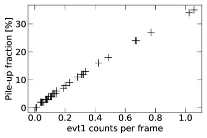
Figure 1: Pile-up fraction versus evt1 counts per frame.

In the case that the pile-up effect can’t be ignored, there are two ways to extract and analyze the X-ray spectrum. One is to extract the spectrum from an annular area by excluding the piled-up core, for example, $0.5-2.0\arcsec$ (e.g., Gambill et al., 2003; Worrall et al., 2004). The other is to fit the spectra extracted from the central region, which includes piled-up core, with $jdppileup$ model (Davis, 2001) in Sherpa. In this work, the latter method was adopted for those spectra extracted from $2.5\arcsec$ circle when the pile-up effect is significant, i.e., evt1 count rate higher than $0.2~{}\rm counts/frame$.

We used Sherpa (Freeman et al., 2001) to fit all X-ray spectra for 3CRR quasars, and two statistical methods were used (see Table 2). One is $cstat$ for the case that the photon count from source-centered $2.5\arcsec$ circle is less than 200, and thus the X-ray spectrum was basically unbinned. The other is $chi2xspecvar$ for the sources with enough exposure time, and the X-ray spectra were binned with 15 counts per bin.

4 Results

4.1 X-ray spectra

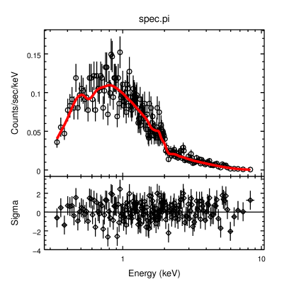
Figure 2: An example of X-ray spectral fitting. A single power-law can fit the spectrum well in 3C 275.1.

The Chandra X-ray spectra extracted from source-centered $2.5\arcsec$ circle were fitted with three models, including intrinsic absorbed power-law model with fixed Galactic absorption ($phabs*zphabs*powerlaw$), absorbed broken power-law model ($phabs*zphabs*bknpower$) and absorbed double power-law model ($phabs*zphabs*(powerlaw1+powerlaw2)$). We found all spectra except for 3C 351 can be best fitted by a single power-law model. As an example, the X-ray spectral fitting for 3C 275.1 is shown in Figure 2. The X-ray spectrum of 3C 351 shows a prominent soft X-ray excess when fitted with the absorbed power-law model, and can be well fitted with a warm absorbed power-law model (see details in Appendix A.1). The X-ray photon index is obtained from the spectral fit for all quasars except for 3C 68.1, in which it was fixed to $\Gamma=1.9$ due to severe absorption (see Appendix A.2). The results of X-ray spectral fitting are shown in Table 2, including X-ray photon index, neutral Hydrogen column density, the absorption-corrected flux at $0.3-2.0~{}\rm keV$, $2.0-10.0~{}\rm keV$ and $0.3-10.0~{}\rm keV$, etc.. The measurement errors of model parameters (e.g., $\Gamma$ and power-law normalization) were estimated with $conf$ script in Sherpa. The flux and its uncertainties were calculated with $sample\_flux$ script in Sherpa.

4.1.1 Compare with other works

There are various works dedicated to detailed spectral analysis on the Chandra data for some of 3CRR quasars with also simple power-law model. Wilkes et al. (2013) extracted X-ray photons from source-centered 2.2″circle and presented the results of X-ray spectral fitting for nine 3CRR quasars (3C 9, 3C 186, 3C 191, 3C 205, 3C 212, 3C 245, 3C 270.1, 3C 287, and 3C 432). We found that the X-ray photon index of their work is consistent with our results within errors. The spectral analysis on three 3CRR quasars (3C 47, 3C 215, 3C 249.1) have been performed by Hardcastle et al. (2006). With extracted X-ray spectra from 1.25″circle, the results of their work are generally in good agreement with our results.

Belsole et al. (2006) and Gambill et al. (2003) studied the X-ray properties for nine quasars (3C 207, 3C 254, 3C 263, 3C 275.1, 3C 309.1, 3C 334, 3C 345, 3C 380, and 3C 454.3). From their results, the fitted X-ray spectra are in general flatter than our results. The difference is likely due to the PSF effect of Chandra/ACIS detector that the harder X-ray has broader PSF, since the central piled-up region was excluded to avoid pile-up effect in their studies. This possibility is supported by our simulation, in which we found flatter X-ray spectra in outer region than inner region (see Appendix B). The K$-$S test shows significantly different distributions of X-ray photon index in two regions. Using the same method to avoid the pile-up effect as Belsole et al. (2006), Hardcastle et al. (2009) presented the slightly flatter photon index than our results for 3C 48, however the result of 3C 325 is same as ours, in which there is no pile-up effect. On the other hand, the similar X-ray photon index with our results have also been found in the sources with pile-up effect, including 3C 48 in Siemiginowska et al. (2008), 3C 254 in Donahue et al. (2003), 3C 263 in Hardcastle et al. (2002), and 3C 454.3 in Tavecchio et al. (2007).

Table 2: The results of X-ray spectral fitting

				$2.5\arcsec$ circle							$log_{10}~{}f~{}(\rm erg~{}cm^{-2}~{}s^{-1})$
Name	$z$	nH	CXO ID	$z$.nH	jdp.a	jdp.f	$\Gamma$	Norm.	$\chi^{2}$/dof.	Stat.	$0.3-2.0~{}\rm keV$	$2.0-10~{}\rm keV$	$0.3-10.0~{}\rm keV$
3C 9	2.012	3.57	1595	$1.45E-02$			$1.61_{-0.08}^{+0.12}$	$0.44_{-0.02}^{+0.04}$	1.48/27	chi2	$-12.90^{+0.07}_{-0.06}$	$-12.69^{+0.16}_{-0.12}$	$-12.48^{+0.11}_{-0.09}$
3C 14	1.469	4.04	9242	$2.54E-01$			$1.53_{-0.18}^{+0.26}$	$1.12_{-0.17}^{+0.31}$	0.71/11	chi2	$-12.51^{+0.10}_{-0.09}$	$-12.24^{+0.23}_{-0.15}$	$-12.05^{+0.16}_{-0.12}$
3C 43	1.470	6.65	9324	$1.04E-03$			$1.53_{-0.15}^{+0.25}$	$0.80_{-0.08}^{+0.20}$	0.78/114	cstat	$-12.65^{+0.04}_{-0.04}$	$-12.37^{+0.12}_{-0.09}$	$-12.19^{+0.08}_{-0.06}$
3C 47	0.425	4.95	2129	$4.15E-02$	0.65	0.94	$1.87_{-0.22}^{+0.21}$	$9.39_{-3.52}^{+2.66}$	1.08/288	chi2	$-11.55^{+0.14}_{-0.14}$	$-11.54^{+0.25}_{-0.17}$	$-11.24^{+0.16}_{-0.14}$
3C 48	0.367	4.34	3097	$0.00E+00$	0.86	0.85	$2.32_{-0.01}^{+0.16}$	$10.65_{-0.20}^{+1.66}$	1.24/171	chi2	$-11.45^{+0.01}_{-0.01}$	$-11.76^{+0.02}_{-0.02}$	$-11.28^{+0.01}_{-0.01}$
3C 68.1	1.238	5.38	9244	$5.31E+00$			$1.90$	$0.55_{-0.12}^{+0.15}$	0.96/39	cstat	$-12.78^{+0.10}_{-0.10}$	$-12.78^{+0.10}_{-0.10}$	$-12.49^{+0.11}_{-0.10}$
3C 138	0.759	21.90	14996	$2.56E-03$	0.80	0.88	$1.46_{-0.11}^{+0.24}$	$3.83_{-0.42}^{+0.99}$	1.80/18	chi2	$-11.97^{+0.06}_{-0.06}$	$-11.63^{+0.10}_{-0.10}$	$-11.48^{+0.08}_{-0.07}$
3C 147	0.545	20.40	14997	$2.02E-01$			$1.85_{-0.22}^{+0.24}$	$2.03_{-0.42}^{+0.55}$	0.75/106	cstat	$-12.22^{+0.11}_{-0.11}$	$-12.19^{+0.24}_{-0.15}$	$-11.90^{+0.14}_{-0.11}$
3C 175	0.768	10.30	14999	$2.45E-03$	0.02	0.85	$1.52_{-0.07}^{+0.40}$	$3.42_{-0.25}^{+0.81}$	0.96/17	chi2	$-12.02^{+0.03}_{-0.03}$	$-11.73^{+0.08}_{-0.07}$	$-11.55^{+0.06}_{-0.05}$
3C 181	1.382	6.63	9246	$2.58E-04$			$1.72_{-0.10}^{+0.17}$	$0.97_{-0.07}^{+0.13}$	1.14/117	cstat	$-12.56^{+0.04}_{-0.04}$	$-12.41^{+0.10}_{-0.08}$	$-12.18^{+0.06}_{-0.05}$
3C 186	1.063	5.11	9774	$1.12E-03$			$1.88_{-0.03}^{+0.05}$	$0.97_{-0.04}^{+0.01}$	1.12/172	chi2	$-12.54^{+0.02}_{-0.02}$	$-12.52^{+0.03}_{-0.03}$	$-12.23^{+0.02}_{-0.02}$
3C 190	1.197	3.04	17107	$1.98E-02$			$1.61_{-0.05}^{+0.06}$	$0.64_{-0.03}^{+0.04}$	1.12/85	chi2	$-12.74^{+0.02}_{-0.02}$	$-12.52^{+0.04}_{-0.04}$	$-12.32^{+0.03}_{-0.03}$
3C 191	1.952	2.45	5626	$1.53E-01$			$1.68_{-0.10}^{+0.11}$	$0.54_{-0.04}^{+0.05}$	0.88/38	chi2	$-12.81^{+0.04}_{-0.04}$	$-12.64^{+0.09}_{-0.07}$	$-12.42^{+0.06}_{-0.05}$
3C 196	0.871	4.82	15001	$2.36E+00$			$1.67_{-0.38}^{+0.40}$	$1.43_{-0.52}^{+0.84}$	0.84/71	cstat	$-12.38^{+0.20}_{-0.19}$	$-12.24^{+0.49}_{-0.25}$	$-11.99^{+0.33}_{-0.20}$
3C 204	1.112	4.59	9248	$3.18E-01$	1.00	1.00	$2.15_{-0.22}^{+0.14}$	$2.41_{-0.32}^{+0.29}$	0.96/156	cstat	$-12.11^{+0.12}_{-0.13}$	$-12.29^{+0.16}_{-0.14}$	$-11.89^{+0.13}_{-0.15}$
3C 205	1.534	4.48	9249	$4.29E-01$	1.00	1.00	$1.83_{-0.17}^{+0.06}$	$1.78_{-0.21}^{+0.12}$	0.94/52	chi2	$-12.28^{+0.05}_{-0.05}$	$-12.23^{+0.05}_{-0.07}$	$-11.96^{+0.05}_{-0.05}$
3C 207	0.684	4.27	2130	$1.98E-01$	0.62	0.86	$1.59_{-0.23}^{+0.08}$	$3.43_{-0.25}^{+14.98}$	0.96/150	chi2	$-12.02^{+0.13}_{-0.12}$	$-11.79^{+0.19}_{-0.15}$	$-11.58^{+0.15}_{-0.13}$
3C 208	1.109	3.12	9250	$1.03E-01$			$1.63_{-0.14}^{+0.18}$	$1.27_{-0.15}^{+0.22}$	0.70/14	chi2	$-12.44^{+0.04}_{-0.04}$	$-12.24^{+0.10}_{-0.08}$	$-12.03^{+0.07}_{-0.06}$
3C 212	1.049	3.79	434	$4.17E-01$	1.00	1.00	$1.85_{-0.08}^{+0.03}$	$3.65_{-0.20}^{+0.11}$	0.73/159	chi2	$-11.97^{+0.01}_{-0.01}$	$-11.93^{+0.01}_{-0.01}$	$-11.65^{+0.01}_{-0.01}$
3C 215	0.411	3.46	3054	$4.58E-02$	0.41	1.00	$1.88_{-0.08}^{+0.09}$	$6.86_{-0.98}^{+0.19}$	0.97/224	chi2	$-11.69^{+0.02}_{-0.02}$	$-11.67^{+0.07}_{-0.05}$	$-11.38^{+0.03}_{-0.03}$
3C 216	0.668	1.30	15002	$2.17E-03$	1.00	1.00	$1.72_{-0.20}^{+0.26}$	$2.16_{-0.25}^{+0.89}$	1.21/10	chi2	$-12.22^{+0.05}_{-0.05}$	$-12.08^{+0.08}_{-0.09}$	$-11.84^{+0.07}_{-0.05}$
3C 245	1.029	2.47	2136	$0.00E+00$	0.29	0.85	$1.57_{-0.05}^{+0.10}$	$2.28_{-0.06}^{+0.17}$	1.07/95	chi2	$-12.19^{+0.01}_{-0.01}$	$-11.94^{+0.04}_{-0.03}$	$-11.75^{+0.02}_{-0.02}$
3C 249.1	0.311	2.80	3986	$0.00E+00$	0.65	0.89	$1.92_{-0.04}^{+0.13}$	$6.61_{-1.09}^{+0.41}$	1.04/191	chi2	$-11.71^{+0.07}_{-0.07}$	$-11.72^{+0.08}_{-0.08}$	$-11.41^{+0.08}_{-0.07}$
3C 254	0.734	1.44	2209	$3.66E-02$	1.00	0.88	$1.93_{-0.07}^{+0.10}$	$2.83_{-0.10}^{+14.12}$	0.91/196	chi2	$-12.07^{+0.02}_{-0.02}$	$-12.09^{+0.02}_{-0.02}$	$-11.78^{+0.02}_{-0.02}$
3C 263	0.652	0.90	2126	$0.00E+00$	1.00	0.95	$1.83_{-0.05}^{+0.09}$	$2.97_{-0.05}^{+5.25}$	1.14/199	chi2	$-12.06^{+0.01}_{-0.01}$	$-12.00^{+0.01}_{-0.01}$	$-11.73^{+0.01}_{-0.01}$
3C 268.4	1.400	1.26	9325	$3.88E-04$			$1.45_{-0.12}^{+0.17}$	$1.17_{-0.10}^{+0.17}$	1.59/14	chi2	$-12.49^{+0.04}_{-0.04}$	$-12.15^{+0.11}_{-0.09}$	$-11.99^{+0.08}_{-0.07}$
3C 270.1	1.519	1.24	13906	$1.69E-01$	0.75	0.85	$1.57_{-0.07}^{+0.07}$	$1.43_{-0.05}^{+0.23}$	1.00/245	chi2	$-12.39^{+0.12}_{-0.11}$	$-12.15^{+0.13}_{-0.13}$	$-11.95^{+0.12}_{-0.13}$
3C 275.1	0.557	1.77	2096	$8.56E-02$	1.00	0.85	$1.79_{-0.10}^{+0.11}$	$2.41_{-0.07}^{+0.38}$	1.06/167	chi2	$-12.15^{+0.01}_{-0.01}$	$-12.07^{+0.06}_{-0.06}$	$-11.81^{+0.04}_{-0.03}$
3C 287	1.055	1.03	3103	$1.02E-01$			$1.86_{-0.04}^{+0.04}$	$1.25_{-0.04}^{+0.04}$	0.88/141	chi2	$-12.43^{+0.01}_{-0.01}$	$-12.40^{+0.03}_{-0.03}$	$-12.11^{+0.02}_{-0.02}$
3C 286	0.849	1.20	15006	$6.36E-05$			$2.12_{-0.26}^{+0.51}$	$1.10_{-0.14}^{+0.50}$	0.66/87	cstat	$-12.46^{+0.05}_{-0.04}$	$-12.63^{+0.12}_{-0.10}$	$-12.23^{+0.05}_{-0.05}$
3C 309.1	0.904	2.27	3105	$0.00E+00$	0.99	0.85	$1.57_{-0.02}^{+0.07}$	$3.95_{-0.05}^{+0.30}$	0.72/186	chi2	$-11.95^{+0.01}_{-0.01}$	$-11.70^{+0.02}_{-0.01}$	$-11.51^{+0.01}_{-0.01}$
3C 325	0.860	1.27	4818	$3.01E+00$			$1.45_{-0.20}^{+0.21}$	$0.29_{-0.06}^{+0.08}$	1.33/19	chi2	$-13.10^{+0.11}_{-0.11}$	$-12.77^{+0.22}_{-0.15}$	$-12.60^{+0.16}_{-0.13}$
3C 334	0.555	4.05	2097	$8.38E-03$	1.00	0.86	$1.85_{-0.11}^{+0.18}$	$3.09_{-0.16}^{+0.49}$	1.18/54	chi2	$-12.04^{+0.03}_{-0.03}$	$-12.00^{+0.04}_{-0.04}$	$-11.72^{+0.03}_{-0.03}$
3C 336	0.927	4.44	15008	$2.66E-01$	1.00	0.85	$1.93_{-0.28}^{+0.24}$	$2.16_{-0.34}^{+0.42}$	0.92/125	cstat	$-12.19^{+0.06}_{-0.06}$	$-12.21^{+0.14}_{-0.11}$	$-11.89^{+0.08}_{-0.06}$
3C 343	0.988	2.01	15011	$5.04E-04$			$2.29_{-0.56}^{+0.82}$	$0.04_{-0.01}^{+0.04}$	1.09/11	cstat	$-13.88^{+0.19}_{-0.15}$	$-14.21^{+0.69}_{-0.26}$	$-13.67^{+0.20}_{-0.15}$
3C 345	0.594	1.14	2143	$0.00E+00$	0.79	0.85	$1.69_{-0.02}^{+0.09}$	$8.79_{-0.10}^{+2.59}$	1.04/191	chi2	$-11.60^{+0.02}_{-0.02}$	$-11.44^{+0.02}_{-0.02}$	$-11.21^{+0.02}_{-0.02}$
3C 351	0.371	2.45	435	$3.00E+00$	0.23	0.85	$1.90_{-0.13}^{+0.20}$	$6.71_{-0.99}^{+2.07}$	1.05/112	chi2	$-11.70^{+0.09}_{-0.09}$	$-11.71^{+0.17}_{-0.09}$	$-11.38^{+0.10}_{-0.11}$
4C 16.49	1.296	6.63	9262	$7.22E-04$			$1.83_{-0.12}^{+0.20}$	$0.98_{-0.07}^{+0.16}$	0.87/115	cstat	$-12.54^{+0.04}_{-0.04}$	$-12.49^{+0.10}_{-0.09}$	$-12.21^{+0.06}_{-0.05}$
3C 380	0.691	5.78	3124	$5.22E-02$	0.95	0.85	$1.76_{-0.10}^{+0.12}$	$8.86_{-0.45}^{+4.01}$	1.04/130	chi2	$-11.59^{+0.01}_{-0.01}$	$-11.48^{+0.02}_{-0.02}$	$-11.23^{+0.01}_{-0.01}$
3C 432	1.805	5.65	5624	$4.17E-01$			$1.76_{-0.10}^{+0.10}$	$0.58_{-0.05}^{+0.05}$	1.14/40	chi2	$-12.77^{+0.04}_{-0.04}$	$-12.66^{+0.08}_{-0.07}$	$-12.41^{+0.05}_{-0.05}$
3C 454	1.757	5.26	21403	$3.55E+00$			$1.75_{-0.19}^{+0.20}$	$0.74_{-0.15}^{+0.20}$	0.80/23	chi2	$-12.67^{+0.10}_{-0.10}$	$-12.56^{+0.19}_{-0.14}$	$-12.31^{+0.13}_{-0.11}$
3C 454.3	0.859	6.63	4843	$1.60E-01$	0.37	0.99	$1.67_{-0.05}^{+0.06}$	$39.09_{-20.50}^{+29.26}$	0.94/387	chi2	$-10.93^{+0.27}_{-0.24}$	$-10.74^{+0.27}_{-0.24}$	$-10.53^{+0.28}_{-0.24}$
3C 455	0.543	4.32	15014	$4.53E-03$			$1.65_{-0.21}^{+0.12}$	$0.27_{-0.04}^{+0.04}$	0.78/110	cstat	$-13.11^{+0.06}_{-0.06}$	$-12.92^{+0.19}_{-0.13}$	$-12.70^{+0.12}_{-0.09}$

Note. — Column (1): 3CRR name; Column (2): Redshift; Column (3): Galactic neutral Hydrogen column density (Kalberla et al., 2005), in units of $10^{20}~{}\rm cm^{-2}$; Column (4): Chandra observation ID; Column (5): Intrinsic Hydrogen column density, in units of $10^{22}~{}\rm cm^{-2}$; Columns (6-7): The alpha and f parameters in $Sherpa$ for $jdpileup$ model (Davis, 2001); Column (8): The power-law photon index and 1 $\sigma$ errors; Column (9): The normalization and 1 $\sigma$ errors of power-law component in $10^{-4}\rm~{}photons\,keV^{-1}\,cm^{-2}\,s^{-1}$ at $1~{}\rm keV$; Column (10): Reduced $\chi^{2}$ and degree of freedom; Column (11): The statistical method, chi2 for $chi2xspecvar$, cstat for $cstat$; Columns ($12-14$): The fluxes and 1 $\sigma$ errors after absorption corrections.

4.2 Composite spectra

As shown in S11, the composite spectrum constructed from the median values within frequency bins (e.g., S11) can be used as the representative of the overall SED for the studied sample. The median values at binned frequencies were obtained from the SED normalized to a given optical frequency. For this reason, the optical/infrared SED will be needed in order to estimate the normalized optical flux. Therefore, to construct the composite X-ray spectrum for the sample, we firstly built the $\log(\nu{f}_{\nu})-\log\nu$ SED at optical/infrared and X-ray bands of all quasars by directly calculating the rest-frame flux density $f_{\nu_{obs}(1+z)}$ from observational optical/infrared data $f_{\nu_{obs}}$ in combination with X-ray measurements. As examples, the SEDs of four quasars are shown in Figure 3.

We followed the same method in S11 to construct the composite spectrum. The SED of individual objects was firstly normalized to rest-frame $4215~{}\rm\AA$. The flux density at rest-frame $4215~{}\rm\AA$ was directly estimated from the power-law fit on the optical/infrared data. When $4215~{}\rm\AA$ is covered by SDSS/NED/SSDC data, only these optical data were used in power-law fit. For those quasars at $0.6<z\leq 1.2$, the 2MASS J-band data was added in the fit. For the objects at $1.2<z\leq 2.0$, 2MASS J,H bands were added, and 2MASS J,H,K bands were used when $z>2.0$. In all the cases except for 3C 68.1, the power-law model gave good fit to the continuum. The continuum of 3C 68.1 is convex, thus deviated from power-law (see Figure 3). This is likely caused by heavy extinction as shown in Appendix A.2. Therefore, we fitted the continuum with the log-parabolic model ($f_{\nu}=k\nu^{(a+b\log\nu)}$, Massaro et al., 2004).

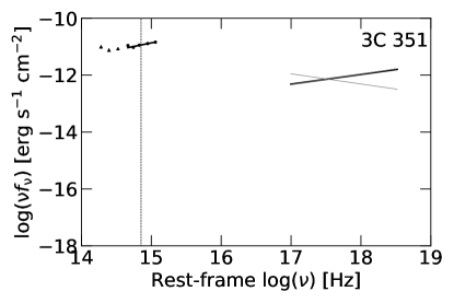
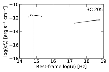
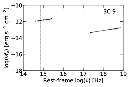
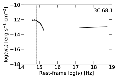
Figure 3: The optical/IR and X-ray SED of four quasars, shown as examples for our sample. The power-law fits are shown in the plots, except for the log parabolic model for optical/IR data of 3C 68.1 (see text for details). The dashed line represents the position of normalization wavelength $4215~{}\rm\AA$.

After normalization, the optical/IR continuum was rebinned with 12 bins in the $\log\nu$ range of 14.7 to 15.3 Hz. This frequency range was selected as it is covered by most quasars. At X-ray band, the spectra were resampled in the $\log\nu$ range of $17.45-18.45$ Hz, with a bin size of $\log\nu=0.1$. Following S11, the composite SED at optical/IR and X-ray band was constructed from the median values in each bin. Two composite median spectra were finally constructed, with one for all 43 3CRR quasars, and the other after excluding six blazars. The composite spectra are shown in Figure 4 with red lines. it can be clearly seen that the composite X-ray spectrum of our 3CRR quasars is very close to the composite spectrum of RLQs in S11, however, it differs that of RQQs in S11 with flatter and stronger hard X-ray emission.

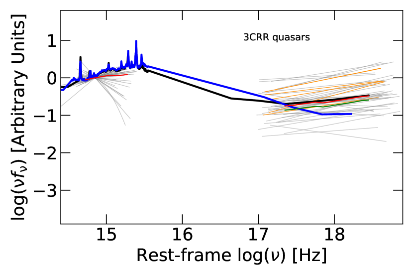
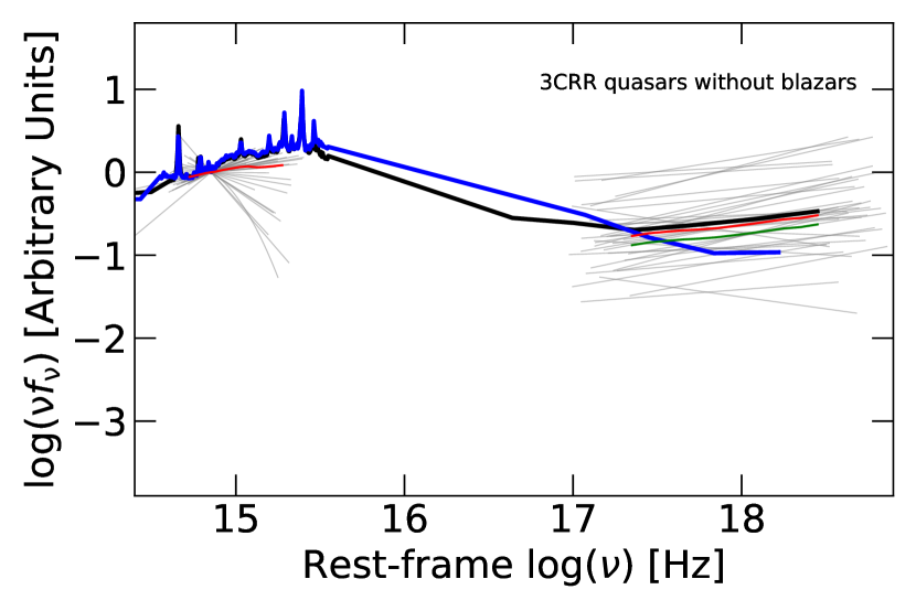
Figure 4: The median composite SED at optical and X-ray bands normalized at 4215$\rm\AA$ for our sample of 3CRR quasars, which are shown in red solid lines. The gray solid lines are normalized SED of individual objects. The thick black and blue solid lines are composite SEDs for RLQs and RQQs in Shang et al. (2011), respectively. The green solid lines are composite X-ray spectra after extinction correction (see text for details). $Upper-$ for all 3CRR quasars, and the orange solid lines are X-ray spectra for six blazars; $Bottom-$ for 3CRR quasars excluding six blazars.

5 Discussions

5.1 Selection effect

There is a well-known relationship between $\alpha_{\rm ox}$ and $L_{2500\rm\AA}$ (e.g., Lusso et al., 2010), in the way that more luminous sources have steeper optical to X-ray slope, which is defined as

$$\alpha_{\rm ox}=-0.384\log(L_{2\rm keV}/L_{2500\rm\AA}).$$ (1)

In this work, the composite X-ray spectrum is constructed using rest-frame $4215~{}\rm\AA$ as a reference, therefore, it will largely depend on the optical/UV luminosity. When comparing with other samples, like S11, this dependence needs to be investigated in order to avoid any selection effects.

In Figure 5, we plotted the relationship between $\alpha_{\rm ox}$ and $L_{2500\rm\AA}$ for our sample and S11 sample. The luminosity at $2500~{}\rm\AA$ of S11 objects is taken from Tang et al. (2012). As Figure 5 shows, 3CRR quasars and S11 RLQs have similar distribution on $\alpha_{\rm ox}-L_{2500\rm\AA}$ panel. However, S11 RQQs have larger $\alpha_{\rm ox}$ (mostly $>1.2$) than that of S11 RLQs and 3CRR quasars. While the $L_{2500\rm\AA}$ luminosity of 3CRR quasars are similar to those of S11 RLQs with Kolmogorov Smirnov (K$-$S) test values $D=0.174$ and $P=0.511$, they are larger than those of S11 RQQs sample with $D=0.632$ and $P=9.536E-06$ from K$-$S test.

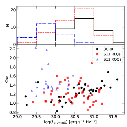
Figure 5: Relation between $\alpha_{\rm ox}$ and luminosity $L_{2500\rm\AA}$ for 3CRR and S11 quasars. The upper panel shows the histogram of luminosity $L_{2500\rm\AA}$.

The similar composite X-ray spectrum of our sample with S11 RLQs seems to be reasonable considering their similar optical/UV luminosity. In contrast, the higher $L_{2500\rm\AA}$ for both samples than S11 RQQs, would imply lower X-ray emission if they follow the general $\alpha_{\rm ox}-L_{2500\rm\AA}$ relation (e.g., Green et al., 1995; Anderson et al., 2003; Vignali et al., 2003). However, this is opposite to our finding, i.e., higher X-ray emission in our sample compared to S11 RQQs. Therefore, the difference between RLQs and RQQs cannot be driven by selection effect related with optical/UV luminosity.

In addition to optical/UV luminosity, we compared black hole mass $M_{\rm BH}$ and Eddington ratio $L_{\rm bol}/L_{\rm Edd}$ of 3CRR quasars with S11 RLQs and RQQs, as shown in Figure 6. The black hole mass and Eddington ratio of S11 quasars were directly taken from Tang et al. (2012). The black hole masses of all 3CRR quasars were obtained from McLure et al. (2006), except for 3C 216 and 3C 345 (Shen et al., 2011), 3C 343 and 3C 455 (Wu, 2009), and 3C 454.3 (Gu et al., 2001). All these virial black hole masses were estimated with the empirical relationship between the broad line region radius and the optical/UV continuum luminosity, in combination with the line width of broad emission lines (e.g., Shen et al., 2011). Depending on source redshift and availability of emission lines, various lines were used in the literature for our sample sources, with H $\beta$ usually at low-redshift sources, while Mg II or C IV at high redshift (see e.g., Shen et al., 2011). We estimated the bolometric luminosity $L_{\rm bol}$ of 3CRR quasars with the relation established from S11 sample in Runnoe et al. (2012),

$$\log(L_{\rm iso})=(4.89\pm 1.66)+(0.91\pm 0.04)\log(\lambda L_{\rm\lambda,5100\AA})$$ (2)

The Eddington luminosity was calculated with black hole mass as $L_{\rm Edd}=1.25\times 10^{38}({M_{\rm BH}}/{M_{\sun}})~{}\rm erg\ s^{-1}$ (Tang et al., 2012).

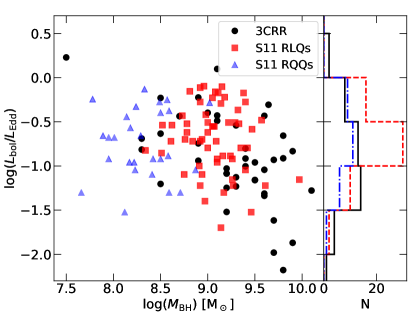
Figure 6: The distribution of black hole mass and Eddington ratio for 3CRR quasars and S11 samples. The right panel shows the histogram of Eddington ratio.

We found from Figure 6 that the Eddington ratio of 3CRR quasars, S11 RLQs and RQQs are similar, although the black hole masses of 3CRR quasars and S11 RLQs are systematically larger than those of S11 RQQs. This implies a similar accretion mode in all three samples. Thus, it further indicates that the difference in composite X-ray spectrum between RLQs and RQQs is not caused by selecting different accretion systems, as manifested from the dependence of $\alpha_{\rm ox}$ on the Eddington ratio (e.g., Ruan et al., 2019).

5.2 Extinction

The advantage of selecting sources at radio band is that the radio emission is not subject to dust extinction, which is in contrast to optical selected sample. We found that the composite optical spectrum of 3CRR quasars is redder than S11 one (see Figure 4). Indeed, we found steep/red optical/UV spectra in many sources (e.g., 3C 14, 3C 68.1, 3C 190, 3C 205, 3C 212, 3C 216, 3C 268.4, 3C 270.1, 3C 325, 3C 343, 3C 345, 3C 454.3 and 3C 455), which can be seen in Figure 4. Prominent absorption lines were found in the optical spectra of many of these quasars, such as Si II, Mg II, C IV, Fe II etc. (e.g., Aldcroft et al., 1994). It seems that there is some absorber locating at the line between source and observer. As the most extreme case, 3C 68.1 is likely a highly inclined and reddened quasar (Boksenberg et al., 1976; Brotherton et al., 1998) as mentioned earlier. 3C 325 is also a reddened quasar classified by Grimes et al. (2005), and its spectrum shows lots of absorption lines in blue side. 3C 270.1 has a steep extreme ultraviolet (EUV) spectrum (Punsly & Marziani, 2015).

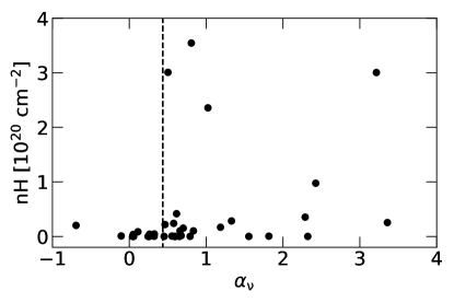
Figure 7: H I column density versus optical spectral index $\alpha_{\rm\nu}$. The dashed line indicates the spectral index of the composite spectrum of S11 RLQs ($\alpha_{\rm\nu}=0.435$).

In Figure 7, we plot the relation of intrinsic H I column density ($\rm nH$, see Table 2) and optical spectral index ($\alpha_{\rm\nu}$) of 3CRR quasars, where $\rm nH$ was calculated from X-ray spectral fitting. We found that the quasars with redder spectra tend to have relatively larger H I column density, supporting dust extinction in some of these objects. If the emission at $4215~{}\rm\AA$ is indeed dust extincted, then the X-ray emission will be overestimated in the composite spectrum.

The systematic extinction of our 3CRR quasar sample can be evaluated by constructing the extinction curve by comparing our composite optical/UV spectrum with that of S11 RLQs sample. We normalized two composite spectra at $\log\nu=14.725~{}\rm Hz$ (i.e., $\lambda=5647.0~{}\rm\AA$, corresponding to the lowest frequency of our composite spectrum). We selected six line-free windows on the composite optical spectrum of S11 RLQs, then a power-law continuum is fitted from these windows (see Figure 8). Using the continuum of S11 RLQs spectrum as reference, the extinction curve of our sample can be obtained, which is shown in Figure 8. We found that the extinction curve is different from the Galactic reddening curve ($R_{\rm V}=3.1$) (Cardelli et al., 1989), SMC extinction curve, and the reddening curve of lobe-dominant radio AGNs in Gaskell et al. (2004), with significantly higher value at short wavelength.

The extinction at $4215~{}\rm\AA$, $A_{4215}$, is tentatively estimated by assuming a selective extinction $R_{\rm V}=3.1$. In this case, we get $A_{4215}=0.272$. Taking this extinction into account, the composite X-ray spectrum will shift down by about 0.11 dex. An adoption of $R_{\rm V}=5.3$ will result in a larger shift of about 0.18 dex. It can be seen from Figure 4 that the X-ray composite spectra after extinction correction are lower than that of S11 RLQs, however the significant difference from S11 RQQs remains.

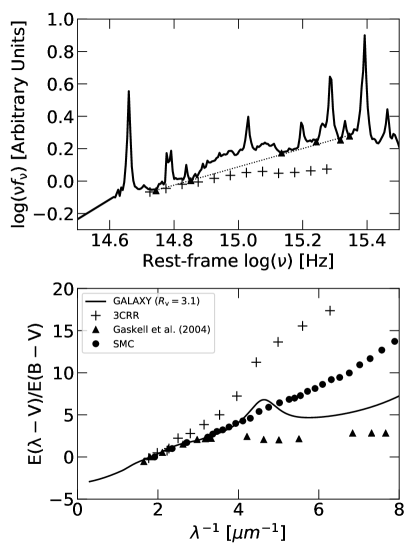
Figure 8: Extinction in 3CRR quasars: ($upper$) - The composite optical/UV spectrum of 3CRR quasars (black crosses) and S11 RLQs (black solid line). The dotted line is the power-law fit on the line-free windows (black triangles) on the S11 RLQs spectrum; ($bottom$) - Extinction curve of 3CRR quasars shown with black crosses. The filled triangles are from the reddening curve of $0.1\leq R_{c}<1$ quasars in Gaskell et al. (2004), where $R_{c}$ is radio core-to-lobe flux ratio. The solid line is Galactic reddening curve of $R_{V}=3.1$. The filled circles show the extinction curve of Small Magellanic Cloud (SMC, Prevot et al., 1984).

5.3 Soft X-ray excess

Compared to S11 RQQs, both composite X-ray spectra of our sample and S11 RLQs show lower soft X-ray emission. This difference may possibly be caused by the low fraction of soft X-ray excess detected in RLQs compared to RQQs (Scott et al., 2011, 2012; Boissay et al., 2016).

There are 27 RQQs in S11, of which 23 sources have available X-ray spectra, 7 from ROSAT and 16 from Chandra or XMM-Newton observations. As shown from the spectra fitting in S11, we found that all ROSAT data were fitted by a single power-law with a steep photon index ($\Gamma>2.43$), and the rest quasars except for PG 0844+349 were fitted by a broken power-law model with a steep photon index at soft X-ray band as to ROSAT data and a flatter photon index at hard X-ray band. PG 0844+349 was fitted by a single power-law in S11, however by a double power-law model in Piconcelli et al. (2005). These results indicate that the soft X-ray excess is likely present in all S11 RQQs with a steeper photon index at soft X-ray band than hard X-ray band. Indeed, we found that RQQs commonly have soft X-ray excess, when we processed the updated Chandra and XMM-Newton data for S11 RQQs sample, which is now available for almost all sources.

As mentioned in Section 4.1, all X-ray spectra of 3CRR quasars except for 3C 351, can be well fitted by a single power-law. This seems to indicate that the soft X-ray excess is likely not evident for our present sample. However, it should be noticed that most of the Chandra observations used in this work arise from the 3CR snapshot survey (Massaro et al., 2010, 2012, 2013, 2018; Stuardi et al., 2018). Therefore, the apparent non-detection of soft X-ray excess may be subject to the low photon counts, which precludes us to do spectral fit in great details.

5.4 X-ray emission in RLQs

It’s well known that the difference of radio emission on the composite SED between RLQs and RQQs (Elvis et al., 1994, S11) can be explained by the presence of powerful relativistic jets in RLQs, which is either weak or absent in RQQs (Panessa et al., 2019). It is conceivable that the jet emission may contribute also at other bands than radio band (e.g., Blandford et al., 2019), especially in blazars when the relativistic jets is moving at small viewing angles (Antonucci, 1993; Urry & Padovani, 1995). While the X-ray emission in RQQs may mainly be from the disk-corona system, the additional contribution from jets may present in RLQs (e.g., Worrall et al., 1987; Miller et al., 2011; Li, 2019). However, the fraction of X-ray emission in radio-loud AGNs that is from the jet, is a strongly debated issue (e.g., Grandi & Palumbo, 2004; Madsen et al., 2015). As illustrated in 3C 273, Grandi & Palumbo (2004) found that the jet emission may contribute at both soft and hard X-ray bands based on the mixture model of Seyfert-like and jet-like emission on the BeppoSAX data, while the jet emission probably only presents at above several tens of keV based on broadband X-ray data, as found in Madsen et al. (2015).

5.4.1 Comparison with previous works

In Figure 4, while our composite X-ray spectrum is similar to that of S11 RLQs, we found that almost all six blazars (3C 207, 3C 216, 3C 309.1, 3C 380, 3C 345, and 3C 454.3) in our sample have higher X-ray flux than the composite spectrum, which may be caused by the significant jet contribution as the jet emission is usually thought to be highly boosted due to “beaming effect”. However, although the X-ray composite spectrum of 3CRR quasars after excluding six blazars is lower than the original one, it is still close to that of S11 RLQs (see Figure 4). The student’s $t$-test shows a significant difference at $>99\%$ confidence level between the distributions of normalized X-ray flux at $\log\nu=18.22$ Hz of 3CRR quasars and S11 RQQs. As a result, the difference of composite X-ray spectrum between RLQs and RQQs is still significant.

The more luminous X-ray in radio-loud AGNs compared to the radio-quiet population, has been also found in many works (e.g., Zamorani et al., 1981; Worrall et al., 1987; Miller et al., 2011). Zamorani et al. (1981) found that RLQs have more X-ray luminosity than RQQs at given optical luminosity. Worrall et al. (1987) suggested that an “extra” X-ray emission would dominate the observed X-ray flux in the majority of RLQs with flat radio spectra. Miller et al. (2011) combined large, modern optical (e.g., SDSS) and radio (e.g., FIRST) surveys with archival X-ray data from Chandra, XMM-Newton, and ROSAT to generate an optically selected sample that includes 188 RIQs and 603 RLQs. The authors found that the excess X-ray luminosity compared to RQQs ranges from $\sim 0.7$ to 2.8 for radio-intermediate quasars through the canonical $\sim 3$ for RLQs to $>10$ for strongly radio-loud or luminous objects. Based on the results, they proposed a model in which the nuclear X-ray emission contains both disk/corona-linked and jet-linked components and demonstrated that the X-ray jet-linked emission is likely beamed but to a lesser degree than applies to the radio jet.

On the other hand, Wilkes & Elvis (1987) found that the X-ray spectral slope of RLQs is flatter than that of RQQs, and argued that the “two-components” model (the flat and the steep components dominate the X-ray flux in RLQs and RQQs, respectively) can explain the result. On the contrary, Sambruna et al. (1999) provided evidence that radio-loud AGNs show comparable distribution of the X-ray continuum slope with radio-quiet AGNs. Similarly, Gupta et al. (2018) found that radio galaxies are on average X-ray-louder than radio-quiet AGNs, however, the spectral slopes of two populations are very similar. The authors argued that in radio-loud and radio-quiet AGNs the hard X-rays are produced in the same region and by the same mechanism. The larger X-ray luminosities in radio-loud AGNs may result from larger radiative efficiencies of the innermost portions of the accretion flows around faster rotating black holes. More recently, Gupta et al. (2020) found that the average X-ray loudness of Type 1 and Type 2 radio-loud AGNs is very similar based on the sample selected from the $Swift$/BAT catalog. The X-ray loudness defined as the ratio of hard X-ray luminosity at 14-195 keV to MIR luminosity can be used to study the orientation-dependent X-ray emission since the MIR radiation is expected to be isotropic (see e.g., Lusso et al., 2013). This similarity indicates negligible dependence of the observed X-ray luminosities on the inclination angle. Therefore, this seems to disfavor the significant jet emission at X-ray band as otherwise the jet emission will be expected to be more significant at smaller viewing angle, then higher X-ray loudness in Type 1 sources. As found in 3C 273, the well-known blazar, the model-fit on the X-ray spectrum from combined observations with Chandra, INTEGRAL, Suzaku, Swift, XMM-Newton, and NuSTAR observatories, gives that the coronal component is fit by $\Gamma_{\rm AGN}=1.638\pm 0.045$, cutoff energy $E_{\rm cutoff}=47\pm 15$ keV, and jet photon index by $\Gamma_{\rm jet}=1.05\pm 0.4$ (Madsen et al., 2015). The beamed jet begins to dominate over emission from the inner accretion flow at $30-40$ keV.

The photon index at $2-10$ keV in our 3CRR quasars ranges from 1.45 to 2.32 with a median value of 1.69. This is in comparable with RQQs (e.g., Wang et al., 2004; Brandt & Alexander, 2015), in good agreement with Gupta et al. (2018) that radio-loud and radio-quiet AGNs have similar distribution of hard X-ray photon index. A significant correlation between the X-ray photon index and the Eddington ratio has been found in radio-quiet AGNs in various works, in which the X-ray emission is thought to be from disk-corona system (e.g., Wang et al., 2004; Brandt & Alexander, 2015). Such correlation if found would be a clue on the emission mechanism of X-ray emission. We plot the relation of the X-ray photon index with the Eddington ratio for our 3CRR quasars sample in Figure 9. There is no significant correlation between the X-ray photon index and the Eddington ratio, in contrast to the finding for RQQs in Wang et al. (2004); Brandt & Alexander (2015). A similar result has also been recently found in Li (2019) for a well-selected sample of radio-loud AGNs. This seems to imply that the X-ray emission may not be from, or at least not be dominated by the disk-corona system. In this case, it seems that the jet contribution can’t be ignored. As a matter of fact, the photon index at $2-10$ keV of our sample is similar to that of FSRQs, which have an average value of $1.65\pm 0.04$ (Donato et al., 2001). However, the large uncertainties in the photon index, probably caused by low data quality, preclude us to draw a firm conclusion.

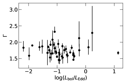
Figure 9: The relation between the X-ray photon index at $2-10~{}\rm keV$ and the Eddington ratio.

5.5 X-ray jets

In principle, the decomposition of X-ray emission into disk-corona and jet component can be performed when a high-quality X-ray spectrum is available at broad bands, as did in 3C 273 (Madsen et al., 2015). However, this is usually hard for sample study due to the lack of broad band data. Although the fraction of X-ray emission in radio-loud AGNs that is from the jet is still unclear, it’s contribution can be studied from the morphology of X-ray emission. Besides the unresolved central X-ray component, the X-ray emission can also be seen from the outer jet as shown in Harris & Krawczynski (2006). The X-ray emission associated with radio jet knots has been studied in details for radio sources in 3CR catalog (Massaro et al., 2015).

XJET (Harris et al., 2010; Massaro et al., 2010, 2011a, 2011b) collected 117 sources, which have extended X-ray emission associated with radio jets. After cross-matching 3CRR quasars with XJET catalog, we found 11 quasars have extended jet component in X-ray images, which has been studied in the literature, including 3C 9 (Fabian et al., 2003), 3C47 (Hardcastle et al., 2004), 3C 207 (Brunetti et al., 2002), 3C 212 (Aldcroft et al., 2003), 3C 254 (Donahue et al., 2003), 3C 263 (Hardcastle et al., 2002), 3C 275.1 (Crawford & Fabian, 2003), 3C 345 (Sambruna et al., 2004), 3C 351 (Brunetti et al., 2001), 3C 380 (Marshall et al., 2005) and 3C 454.3 (Marshall et al., 2005). Moreover, we checked the results of Massaro et al. (2015), and found that six more quasars (3C 181, 3C 191, 3C 215, 3C 245, 3C 325 and 3C 334) may have extended X-ray component related with jet knot, hotspot, or lobe. In addition, the extended X-ray emission from jet has also been found in 3C 270.1 (Wilkes et al., 2012) and 3C 432 (Erlund et al., 2006). In total, there are 19 3CRR quasars having extended X-ray components associated with radio jets.

Massaro et al. (2009) reported the X-ray emission from the radio jet of 3C 17 with Chandra observations, and found that the high energy emission from the jet knots can be explained by both inverse Compton(IC)/cosmic microwave background (CMB) and Synchrotron process. Recently, Mingo et al. (2017) found that the spectral fit of hotspots is consistent with the synchrotron emission, while the IC emission is found for lobes. In the case study of 3C 459, the extended X-ray emission can be well modelled by a plasma collisionally heated by jet-driven shocks (Maselli et al., 2018). Based on the good correlation between the unabsorbed component of X-ray luminosity and the 5-GHz core radio luminosity, Hardcastle et al. (2009) argued that at least some, and in many cases all, of the soft component of radio-source X-ray spectra originates in the jet is very hard to evade for a sample of 3CRR radio sources. As shown in Massaro et al. (2015), jet knot, hotspot, and lobe may all have X-ray emission, therefore, the emission from the jet components in the region of $2.5\arcsec$ radius will contribute in the composite spectrum constructed for our quasar sample. While the central $2.5\arcsec$ is unresolved in X-ray image, it can be usually resolved into core-jet structure with a central bright core and several jet components at radio band (e.g., 3C 245, see Figure 1 in Massaro et al., 2015). When the X-ray emission is extracted in central $2.5\arcsec$, the X-ray emission associated with jet components will naturally be included, although their flux fractions are largely unknown. As an additional check of jet emission at X-ray band, we studied the X-ay emission at different regions. However, no strong evidence of jet contribution was found due to the large uncertainties in the X-ray photon index (see Appendix B).

6 Summary

In this work, we revisited the difference of composite X-ray spectrum between RLQs and RQQs, by using multi-band data for 3CRR quasars sample, which was selected at low radio frequency, thus less affected by the “beaming effect”. We found that the composite X-ray spectrum of 3CRR quasars is similar to S11 RLQs after excluding blazars, still significantly different from RQQs. Although the photon index at $2-10$ keV of our sample is similar to RQQs, there is no strong correlation between the photon index and Eddington ratio, implying that other emission than the one from disk-corona system may also contribute at X-ray band, presumably from jet. The detection of X-ray emission from jet components has been reported in many sources from the literature, and the jet components might be included in extracting the X-ray spectrum from the central $2.5\arcsec$ region. Our results suggest that the jet emission at X-ray band in RLQs could be related with the difference of composite X-ray spectrum between RLQs and RQQs.

Appendix A The X-ray spectral fit

A.1 3C 351

3C 351 ($z=0.371$) has been observed by Chandra twice, a 9.15 ks observation with ID 435 on June 1, 2000, and a 50.92 ks observation with ID 2128 on August 24, 2001. These data were processed with CIAO as in Section 3.2. The evt1 file counts per frame in $1.5\arcsec$ region are 0.142 and $0.327~{}\rm counts/frame$, for 435 and 2128 data, respectively. Therefore, the pile-up effect might be taken into account for the spectrum of 2128. We fitted these two spectra with absorbed power-law model and found that both spectra cannot be fitted well with significant excess at soft X-ray band (see the left panel in Figure 10).

The soft X-ray spectrum of 3C 351 has been investigated by Fiore et al. (1993) using ROSAT data. The authors found that partial covering, soft excess, and warm absorber models can all fit the spectrum well, although only the warm absorber model (i.e., partially ionized absorbing material in the line of sight) gives a good $\chi^{2}$ for a typical value of high energy continuum slope. If the warm absorber model is correct, the strongest absorption edge lies in the range $0.58-0.76~{}\rm keV$, implying O IV$-$O VII as the most likely absorbing ions. Mathur et al. (1994) provided strong evidence for the warm absorber model in the soft X-ray spectrum.

As did in Fiore et al. (1993), we fitted the spectra of 3C 351 with the warm absorbed power-law model ($phabs*zxipcf*powerlaw$) using $chi2xspecvar$ statistical method. Here, we set the nH of photo-electric absorption ($phabs$) to Galactic H I column density (Kalberla et al., 2005) and $zxipcf$ redshift to 0.371. We found two Chandra spectra can be well fitted by the model. As shown in the right panel of Figure 10, the prominent absorption edge is visible below $1~{}\rm keV$. The results of spectral fitting are given in Table 3.

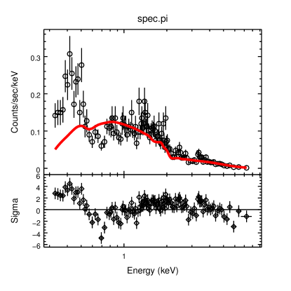
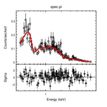
Figure 10: 3C 351 spectrum of Chandra observation ID 435: ($Left$) - The spectrum is fitted by the absorbed power-law model ($phabs*zphabs*powerlaw$); ($Right$) - The spectrum is fitted with the warm absorbed power-law model ($phabs*zxipcf*powerlaw$).

Table 3: The spectral fitting for 3C 351

		$435$	$2128$
pile-up	alpha		0.42
	f		1.00
zxipcf	nH($\rm 10^{22}~{}cm^{-2}$)	3.00	2.96
	$\log(xi)$	1.90	1.20
	Covering Fraction	1.00	0.90
Power-law	$\Gamma$	$1.66_{-0.03}^{+0.70}$	$1.96_{-0.12}^{+0.13}$
	Norm. ($10^{-4}$)	$4.54_{-0.12}^{+7.96}$	$6.87_{-1.21}^{+0.56}$
	$\chi^{2}_{Red}/dof.$	$1.10/114$	$1.05/232$
Flux	$0.3-2.0~{}\rm keV$	$-11.89^{+0.01}_{-0.01}$	$-11.68^{+0.02}_{-0.02}$
	$2.0-10.0~{}\rm keV$	$-11.70^{+0.02}_{-0.02}$	$-11.72^{+0.04}_{-0.04}$
	$0.3-10.0~{}\rm keV$	$-11.49^{+0.01}_{-0.01}$	$-11.40^{+0.02}_{-0.02}$

Note. — Rows 1 and 2: pile-up parameters; Rows $3-5$: $zxipcf$ parameters; Rows $6-8$: power-law parameters, where $\Gamma$ is photon index, Norm. is $\rm photons\,keV^{-1}\,cm^{-2}\,s^{-1}$ at $1~{}\rm keV$, and $\chi^{2}_{Red}/dof.$ is reduced $\chi^{2}$ and degree of freedom; Rows $9-11$: the absorption-corrected flux ($\log f$ in units of $\rm erg~{}cm^{-2}~{}s^{-1}$).

A.2 3C 68.1

3C 68.1 is an optically red quasar with very steep optical spectrum ($\alpha\sim 6.1$) (Boksenberg et al., 1976), and is also highly polarized at $3000-8000~{}\rm\AA$ (Moore & Stockman, 1981, 1984). Brotherton et al. (1998) argued that 3C 68.1 is a highly inclined quasar and shows intrinsic ultraviolet absorption lines, like, Mg II, and Ca II K. 3C 68.1 probably has absorbed X-ray emission (Bregman et al., 1985). All these observational features indicate that 3C 68.1 is likely an edge-on system along a line of sight through dusty, and ionized gas, perhaps part of torus (Brotherton et al., 2002).

3C 68.1 has been observed with an exposure time of $3.05~{}\rm ks$ by Chandra on February 10, 2008 (ID: 9244). The X-ray spectrum extracted from $2.5\arcsec$ circle was fitted with an absorbed power-law model with fixed Galactic absorption ($phabs*zphabs*powerlaw$). An extremely flat spectrum was found with $\Gamma=0.46_{-0.33}^{+0.41}$. The flat X-ray spectrum is consistent with the finding in Goulding et al. (2018) for extremely red quasars, and it may imply severe absorption in the source as shown from the extremely red optical spectrum and intrinsic ultraviolet absorption. Therefore, we fitted the X-ray spectrum again by fixing $\Gamma=1.9$, and found the intrinsic X-ray absorption of $N_{H}\sim 5.31\times 10^{22}~{}\rm cm^{-2}$.

Appendix B X-ray emission at different regions

To further get the clues of jet contribution at X-ray band, we tried to compare the X-ray spectra extracted from different regions, $0.5-2.0\arcsec$ annulus and central $1.5\arcsec$, in which the jet contribution is expected to be different. 3C 68.1 and 3C 343 are excluded due to low photon counts in $0.5-2.0\arcsec$ annulus. We found that all Chandra X-ray spectra can be well fitted by absorbed power-law model except for 3C 351 (see Table 4).

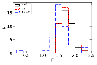
Figure 11: The distribution of X-ray photon index $\Gamma$. The solid line is for $2.5\arcsec$ region, and the dashed line represents $1.5\arcsec$ region. As comparison, the $0.5-2.0\arcsec$ annulus is shown as dot-dashed line.

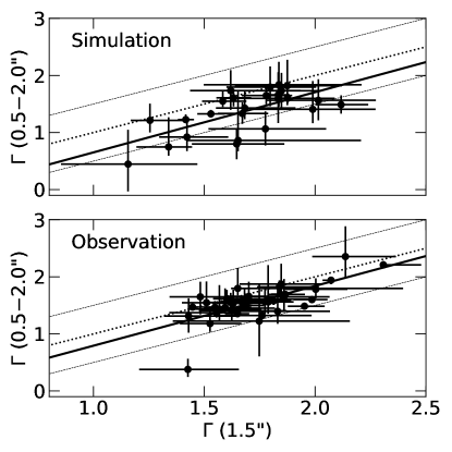
Figure 12: The relation of the X-ray photon index from $1.5\arcsec$ circle and from $0.5-2.0\arcsec$ annulus: ($upper$) - simulation; ($bottom$) - observation. The black dotted line is equivalent line, and its 0.5 offset is shown as dashed lines. The black solid lines show the linear fit.

The distribution of X-ray photon index at $2-10$ keV from $0.5-2.0\arcsec$, $1.5\arcsec$ and $2.5\arcsec$ are compared in Figure 11. While the photon index of $1.5\arcsec$ is similar to that of $2.5\arcsec$, we found that most sources (34/41) have flatter spectra from outer region ($0.5-2.0\arcsec$ annulus) than inner region ($1.5\arcsec$ circle). While this may be caused by the intrinsic difference in the emission at different regions, the effect that Chandra/ACIS detector has broader PSF at hard X-ray can’t be ignored. To examine the PSF effect, we used MARX simulate events on the X-ray data of our sample. After excluding the sources with pile-up effect, and low photon counts data, we extracted the X-ray spectra of 26 quasars from the source-centered region with $5\arcsec$ radius out of background region ($5-20\arcsec$ annulus) and fitted them with 1-D polynomial function ($polynom1d$), which were used as input spectra to MARX. The X-ray spectra of source-centered $1.5\arcsec$ circle and $0.5-2.0\arcsec$ annulus extracted from simulated data were fitted with an absorbed power-law model ($phabs*powerlaw$). We found the X-ray spectra from outer region are flatter than those from inner region, with median photon index of 1.49 and 1.68 for the former and the latter, respectively. The K$-$S test shows significantly different distributions of X-ray photon index in two regions with $D=0.440$ and $P=0.010$. The resulting photon index at $2-10~{}\rm keV$ is shown in Figure 12. Indeed, the PSF effect results in flatter spectra in outer region than inner region, which even is more significant than the observational result. Therefore, by taking this PSF effect into account, the X-ray spectra at outer region is slightly steeper than inner region. However, the firm conclusion can’t be drawn due to the large uncertainties in the photon index.

Table 4: The X-ray spectral fitting for different regions

			$1.5\arcsec$ circle			$0.5-2.0\arcsec$ annulus
Name	CXO ID	$\Gamma_{0}$	$\Gamma_{1}$	$\chi^{2}_{Red}/dof.$	Stat.	$\Gamma_{2}$	$\chi^{2}_{Red}/dof.$	Stat.
3C 9	1595	$1.61_{-0.08}^{+0.12}$	$1.62_{-0.10}^{+0.12}$	1.29/27	chi2	$1.55_{-0.16}^{+0.17}$	0.90/111	cstat
3C 14	9242	$1.53_{-0.18}^{+0.26}$	$1.43_{-0.11}^{+0.22}$	0.90/11	chi2	$1.31_{-0.29}^{+0.31}$	0.95/52	cstat
3C 43	9324	$1.53_{-0.15}^{+0.25}$	$1.48_{-0.14}^{+0.27}$	0.95/110	cstat	$1.65_{-0.31}^{+0.27}$	1.07/34	cstat
3C 47	2129	$1.87_{-0.22}^{+0.21}$	$1.76_{-0.20}^{+0.22}$	1.08/282	chi2	$1.32_{-0.04}^{+0.06}$	1.13/128	chi2
3C 48	3097	$2.32_{-0.01}^{+0.16}$	$2.31_{-0.01}^{+0.17}$	1.24/170	chi2	$2.21_{-0.03}^{+0.07}$	0.84/94	chi2
3C 138	14996	$1.46_{-0.11}^{+0.24}$	$1.59_{-0.10}^{+0.12}$	1.05/205	cstat	$1.46_{-0.11}^{+0.33}$	0.89/97	cstat
3C 147	14997	$1.85_{-0.22}^{+0.24}$	$1.83_{-0.22}^{+0.24}$	0.75/106	cstat	$1.40_{-0.22}^{+0.40}$	1.00/38	cstat
3C 175	14999	$1.57_{-0.10}^{+0.11}$	$1.51_{-0.11}^{+0.13}$	0.57/18	chi2	$1.55_{-0.14}^{+0.37}$	0.86/85	cstat
3C 181	9246	$1.72_{-0.10}^{+0.17}$	$1.70_{-0.10}^{+0.15}$	1.14/116	cstat	$1.66_{-0.20}^{+0.26}$	1.13/49	cstat
3C 186	9774	$2.08_{-0.03}^{+0.06}$	$2.07_{-0.04}^{+0.02}$	0.99/165	chi2	$1.94_{-0.07}^{+0.04}$	1.04/88	chi2
3C 190	17107	$1.61_{-0.05}^{+0.06}$	$1.60_{-0.06}^{+0.07}$	1.17/79	chi2	$1.62_{-0.06}^{+0.15}$	0.81/33	chi2
3C 191	5626	$1.68_{-0.10}^{+0.11}$	$1.68_{-0.10}^{+0.11}$	0.98/36	chi2	$1.57_{-0.11}^{+0.14}$	0.93/14	chi2
3C 196	15001	$1.67_{-0.38}^{+0.40}$	$1.75_{-0.39}^{+0.41}$	0.89/68	cstat	$1.22_{-0.62}^{+0.66}$	1.02/24	cstat
3C 204	9248	$1.95_{-0.14}^{+0.14}$	$2.00_{-0.14}^{+0.14}$	0.98/154	cstat	$1.78_{-0.16}^{+0.19}$	0.99/75	cstat
3C 205	9249	$1.66_{-0.09}^{+0.09}$	$1.68_{-0.09}^{+0.09}$	0.84/53	chi2	$1.60_{-0.20}^{+0.21}$	1.15/14	chi2
3C 207	2130	$1.59_{-0.23}^{+0.08}$	$1.56_{-0.21}^{+0.10}$	0.95/147	chi2	$1.37_{-0.09}^{+0.09}$	1.00/51	chi2
3C 208	9250	$1.63_{-0.14}^{+0.18}$	$1.63_{-0.08}^{+0.13}$	0.91/15	chi2	$1.54_{-0.14}^{+0.24}$	0.63/69	cstat
3C 212	434	$1.68_{-0.04}^{+0.04}$	$1.67_{-0.04}^{+0.04}$	0.74/159	chi2	$1.57_{-0.08}^{+0.08}$	1.22/60	chi2
3C 215	3054	$1.88_{-0.08}^{+0.09}$	$1.87_{-0.08}^{+0.09}$	0.94/223	chi2	$1.69_{-0.05}^{+0.06}$	0.92/124	chi2
3C 216	15002	$1.59_{-0.13}^{+0.26}$	$1.62_{-0.15}^{+0.25}$	1.14/12	chi2	$1.41_{-0.17}^{+0.27}$	0.93/63	cstat
3C 245	2136	$1.55_{-0.03}^{+0.06}$	$1.55_{-0.03}^{+0.06}$	1.06/95	chi2	$1.47_{-0.09}^{+0.11}$	0.74/33	chi2
3C 249.1	3986	$1.92_{-0.04}^{+0.13}$	$1.99_{-0.08}^{+0.07}$	1.09/188	chi2	$1.60_{-0.05}^{+0.05}$	0.98/93	chi2
3C 254	2209	$1.93_{-0.07}^{+0.10}$	$1.95_{-0.08}^{+0.09}$	0.90/192	chi2	$1.49_{-0.03}^{+0.06}$	1.05/101	chi2
3C 263	2126	$1.83_{-0.05}^{+0.09}$	$1.81_{-0.08}^{+0.08}$	1.02/197	chi2	$1.58_{-0.07}^{+0.05}$	1.57/78	chi2
3C 268.4	9325	$1.45_{-0.12}^{+0.17}$	$1.53_{-0.14}^{+0.14}$	0.90/160	cstat	$1.18_{-0.15}^{+0.22}$	0.95/70	cstat
3C 270.1	13906	$1.57_{-0.07}^{+0.07}$	$1.58_{-0.07}^{+0.07}$	1.00/243	chi2	$1.42_{-0.05}^{+0.05}$	0.91/118	chi2
3C 275.1	2096	$1.79_{-0.10}^{+0.11}$	$1.79_{-0.10}^{+0.11}$	1.01/166	chi2	$1.56_{-0.07}^{+0.07}$	0.86/66	chi2
3C 287	3103	$1.86_{-0.04}^{+0.04}$	$1.84_{-0.04}^{+0.04}$	0.86/140	chi2	$1.70_{-0.08}^{+0.08}$	0.98/60	chi2
3C 286	15006	$2.12_{-0.26}^{+0.51}$	$2.14_{-0.15}^{+0.23}$	0.67/86	cstat	$2.35_{-0.38}^{+0.53}$	0.94/27	cstat
3C 309.1	3105	$1.46_{-0.01}^{+0.09}$	$1.45_{-0.01}^{+0.10}$	0.77/187	chi2	$1.47_{-0.04}^{+0.04}$	1.09/87	chi2
3C 325	4818	$1.45_{-0.20}^{+0.21}$	$1.43_{-0.22}^{+0.23}$	0.81/18	chi2	$0.38_{-0.13}^{+0.19}$	1.09/89	cstat
3C 334	2097	$1.85_{-0.11}^{+0.18}$	$1.84_{-0.10}^{+0.18}$	1.17/52	chi2	$1.82_{-0.12}^{+0.12}$	1.55/17	chi2
3C 336	15008	$1.82_{-0.18}^{+0.18}$	$1.85_{-0.19}^{+0.18}$	0.94/124	cstat	$1.87_{-0.20}^{+0.36}$	1.05/50	cstat
3C 345	2143	$1.69_{-0.02}^{+0.09}$	$1.68_{-0.02}^{+0.09}$	1.08/190	chi2	$1.50_{-0.02}^{+0.08}$	0.85/96	chi2
3C 351	435	$1.66_{-0.03}^{+0.70}$	$1.65_{-0.03}^{+0.75}$	1.10/112	chi2	$1.80_{-0.12}^{+0.36}$	1.03/38	chi2
4C 16.49	9262	$1.83_{-0.12}^{+0.20}$	$1.86_{-0.14}^{+0.21}$	0.90/111	cstat	$1.65_{-0.23}^{+0.31}$	1.06/49	cstat
3C 380	3124	$1.76_{-0.10}^{+0.12}$	$1.67_{-0.10}^{+0.15}$	0.99/129	chi2	$1.45_{-0.04}^{+0.09}$	0.97/57	chi2
3C 432	5624	$1.76_{-0.10}^{+0.10}$	$1.77_{-0.10}^{+0.10}$	1.14/39	chi2	$1.56_{-0.21}^{+0.22}$	0.96/15	chi2
3C 454	21403	$1.75_{-0.19}^{+0.20}$	$1.78_{-0.20}^{+0.21}$	0.92/22	chi2	$1.61_{-0.26}^{+0.59}$	0.99/106	cstat
3C 454.3	4843	$1.67_{-0.05}^{+0.06}$	$1.65_{-0.06}^{+0.05}$	1.01/383	chi2	$1.35_{-0.03}^{+0.03}$	0.98/225	chi2
3C 455	15014	$1.65_{-0.21}^{+0.12}$	$1.57_{-0.14}^{+0.19}$	0.78/108	cstat	$1.43_{-0.22}^{+0.42}$	1.07/49	cstat

Note. — Column (1): 3CRR name; Column (2): Chandra observation ID; Column (3): Photon index of power-law component extracted from source-centered $2.5\arcsec$ circle; Column ($4-6$): Photon index, reduced $\chi^{2}$/degree of freedom and statistical method for the power-law fit in $1.5\arcsec$ circle; Columns ($7-9$): The power-law fit in $0.5-2.0\arcsec$ annulus.

References

- Aars et al. (2005) Aars, C. E., Hough, D. H., Yu, L. H., et al. 2005, AJ, 130, 23
- Abazajian et al. (2009) Abazajian, K. N., Adelman-McCarthy, J. K., Agüeros, M. A., et al. 2009, ApJS, 182, 543
- Alam et al. (2015) Alam, S., Albareti, F. D., Allende Prieto, C., et al. 2015, ApJS, 219, 12
- Alexander et al. (2013) Alexander, D. M., Stern, D., Del Moro, A., et al. 2013, ApJ, 773, 125
- Aldcroft et al. (1994) Aldcroft, T. L., Bechtold, J., & Elvis, M. 1994, ApJS, 93, 1
- Aldcroft et al. (1993) Aldcroft, T. L., Elvis, M., & Bechtold, J. 1993, AJ, 105, 2054
- Aldcroft et al. (2003) Aldcroft, T. L., Siemiginowska, A., Elvis, M., et al. 2003, ApJ, 597, 751
- Anderson et al. (2003) Anderson, S. F., Voges, W., Margon, B., et al. 2003, AJ, 126, 2209
- Antonucci (1993) Antonucci, R. 1993, ARA&A, 31, 473
- Ballantyne et al. (2002) Ballantyne, D. R., Ross, R. R., & Fabian, A. C. 2002, MNRAS, 332, L45
- Bedford et al. (1981) Bedford, N. H., Kerr, A. J., Mathur, S. H., et al. 1981, MNRAS, 195, 245
- Belsole et al. (2006) Belsole, E., Worrall, D. M., & Hardcastle, M. J. 2006, MNRAS, 366, 339
- Blandford et al. (2019) Blandford, R., Meier, D., & Readhead, A. 2019, ARA&A, 57, 467
- Boissay et al. (2016) Boissay, R., Ricci, C., & Paltani, S. 2016, A&A, 588, A70
- Boksenberg et al. (1976) Boksenberg, A., Carswell, R. F., & Oke, J. B. 1976, ApJ, 206, L121
- Brandt & Alexander (2015) Brandt, W. N., & Alexander, D. M. 2015, A&A Rev., 23, 1
- Brandt & Hasinger (2005) Brandt, W. N., & Hasinger, G. 2005, ARA&A, 43, 827
- Bregman et al. (1985) Bregman, J. N., Glassgold, A. E., Huggins, P. J., & Kinney, A. L. 1985, ApJ, 291, 505
- Bridle et al. (1994) Bridle, A. H., Hough, D. H., Lonsdale, C. J., Burns, J. O., & Laing, R. A. 1994, AJ, 108, 766
- Brotherton et al. (1998) Brotherton, M. S., Wills, B. J., Dey, A., van Breugel, W., & Antonucci, R. 1998, ApJ, 501, 110
- Brotherton et al. (2002) Brotherton, M. S., Ly, C., Wills, B. J., et al. 2002, AJ, 124, 1943
- Brunetti et al. (2001) Brunetti, G., Bondi, M., Comastri, A., et al. 2001, ApJ, 561, L157
- Brunetti et al. (2002) Brunetti, G., Bondi, M., Comastri, A., & Setti, G. 2002, A&A, 381, 795
- Cardelli et al. (1989) Cardelli, J. A., Clayton, G. C., & Mathis, J. S. 1989, Interstellar Dust, 135, 5
- Cohen et al. (2003) Cohen, M., Wheaton, W. A., & Megeath, S. T. 2003, AJ, 126, 1090
- Crawford & Fabian (2003) Crawford, C. S., & Fabian, A. C. 2003, MNRAS, 339, 1163
- Croston et al. (2005) Croston, J. H., Hardcastle, M. J., Harris, D. E., et al. 2005, ApJ, 626, 733
- Crummy et al. (2006) Crummy, J., Fabian, A. C., Gallo, L., & Ross, R. R. 2006, MNRAS, 365, 1067
- Cutri et al. (2003) Cutri, R. M., Skrutskie, M. F., van Dyk, S., et al. 2003, The IRSA 2MASS All-Sky Point Source Catalog
- Davis (2001) Davis, J. E. 2001, ApJ, 562, 575
- Dewangan et al. (2007) Dewangan, G. C., Griffiths, R. E., Dasgupta, S., & Rao, A. R. 2007, ApJ, 671, 1284
- Dickey & Lockman (1990) Dickey, J. M., & Lockman, F. J. 1990, ARA&A, 28, 215
- Donahue et al. (2003) Donahue, M., Daly, R. A., & Horner, D. J. 2003, ApJ, 584, 643
- Donato et al. (2001) Donato, D., Ghisellini, G., Tagliaferri, G., & Fossati, G. 2001, A&A, 375, 739
- Done et al. (2012) Done, C., Davis, S. W., Jin, C., Blaes, O., & Ward, M. 2012, MNRAS, 420, 1848
- Elvis et al. (1994) Elvis, M., Wilkes, B. J., McDowell, J. C., et al. 1994, ApJS, 95, 1
- Erlund et al. (2006) Erlund, M. C., Fabian, A. C., Blundell, K. M., Celotti, A., & Crawford, C. S. 2006, MNRAS, 371, 29
- Fabian et al. (2002) Fabian, A. C., Ballantyne, D. R., Merloni, A., et al. 2002, MNRAS, 331, L35
- Fabian et al. (2003) Fabian, A. C., Celotti, A., & Johnstone, R. M. 2003, MNRAS, 338, L7
- Fan & Zhang (2003) Fan, J. H., & Zhang, J. S. 2003, A&A, 407, 899
- Fanaroff & Riley (1974) Fanaroff, B. L., & Riley, J. M. 1974, MNRAS, 167, 31P
- Fernini et al. (1997) Fernini, I., Burns, J. O., & Perley, R. A. 1997, AJ, 114, 2292
- Fernini (2007) Fernini, I. 2007, AJ, 134, 158
- Fernini (2014) Fernini, I. 2014, ApJS, 212, 19
- Fiore et al. (1993) Fiore, F., Elvis, M., Mathur, S., Wilkes, B. J., & McDowell, J. C. 1993, ApJ, 415, 129
- Freeman et al. (2001) Freeman, P., Doe, S., & Siemiginowska, A. 2001, Proc. SPIE, 4477, 76
- Fruscione et al. (2006) Fruscione, A., McDowell, J. C., Allen, G. E., et al. 2006, Proc. SPIE, 6270, 62701V
- Gambill et al. (2003) Gambill, J. K., Sambruna, R. M., Chartas, G., et al. 2003, A&A, 401, 505
- García et al. (2014) García, J., Dauser, T., Lohfink, A., et al. 2014, ApJ, 782, 76
- Gaskell et al. (2004) Gaskell, C. M., Goosmann, R. W., Antonucci, R. R. J., & Whysong, D. H. 2004, ApJ, 616, 147
- Goulding et al. (2018) Goulding, A. D., Zakamska, N. L., Alexandroff, R. M., et al. 2018, ApJ, 856, 4
- Grandi et al. (2006) Grandi, P., Malaguti, G., & Fiocchi, M. 2006, ApJ, 642, 113
- Grandi & Palumbo (2004) Grandi, P., & Palumbo, G. G. C. 2004, Science, 306, 998
- Green et al. (1995) Green, P. J., Schartel, N., Anderson, S. F., et al. 1995, ApJ, 450, 51
- Grimes et al. (2005) Grimes, J. A., Rawlings, S., & Willott, C. J. 2005, MNRAS, 359, 1345
- Gu et al. (2001) Gu, M., Cao, X., & Jiang, D. R. 2001, MNRAS, 327, 1111
- Gupta et al. (2018) Gupta, M., Sikora, M., Rusinek, K., & Madejski, G. M. 2018, MNRAS, 480, 2861
- Gupta et al. (2020) Gupta, M., Sikora, M., & Rusinek, K. 2020, MNRAS, 492, 315
- Gürkan et al. (2014) Gürkan, G., Hardcastle, M. J., & Jarvis, M. J. 2014, MNRAS, 438, 1149
- Haardt & Maraschi (1993) Haardt, F., & Maraschi, L. 1993, ApJ, 413, 507
- Haas et al. (2004) Haas, M., Müller, S. A. H., Bertoldi, F., et al. 2004, A&A, 424, 531
- Haas et al. (2008) Haas, M., Willner, S. P., Heymann, F., et al. 2008, ApJ, 688, 122-127
- Hardcastle et al. (2002) Hardcastle, M. J., Birkinshaw, M., Cameron, R. A., et al. 2002, ApJ, 581, 948
- Hardcastle et al. (2006) Hardcastle, M. J., Evans, D. A., & Croston, J. H. 2006, MNRAS, 370, 1893
- Hardcastle et al. (2009) Hardcastle, M. J., Evans, D. A., & Croston, J. H. 2009, MNRAS, 396, 1929
- Hardcastle et al. (2004) Hardcastle, M. J., Harris, D. E., Worrall, D. M., & Birkinshaw, M. 2004, ApJ, 612, 729
- Harris & Krawczynski (2006) Harris, D. E., & Krawczynski, H. 2006, ARA&A, 44, 463
- Harris et al. (2010) Harris, D. E., Massaro, F., & Cheung, C. C. 2010, X-ray Astronomy 2009; Present Status, Multi-wavelength Approach and Future Perspectives, 355
- Healey et al. (2007) Healey, S. E., Romani, R. W., Taylor, G. B., et al. 2007, ApJS, 171, 61
- Jin et al. (2017) Jin, C., Done, C., & Ward, M. 2017, MNRAS, 468, 3663
- Kalberla et al. (2005) Kalberla, P. M. W., Burton, W. B., Hartmann, D., et al. 2005, A&A, 440, 775
- Kataoka et al. (2011) Kataoka, J., Stawarz, Ł., Takahashi, Y., et al. 2011, ApJ, 740, 29
- Kellermann et al. (1989) Kellermann, K. I., Sramek, R., Schmidt, M., et al. 1989, AJ, 98, 1195
- Krawczyk et al. (2013) Krawczyk, C. M., Richards, G. T., Mehta, S. S., et al. 2013, ApJS, 206, 4
- Laing et al. (1983) Laing, R. A., Riley, J. M., & Longair, M. S. 1983, MNRAS, 204, 151
- Laurent-Muehleisen et al. (1997) Laurent-Muehleisen, S. A., Kollgaard, R. I., Ryan, P. J., et al. 1997, A&AS, 122, 235
- Lehnert et al. (1999) Lehnert, M. D., Miley, G. K., Sparks, W. B., et al. 1999, ApJS, 123, 351
- Li (2019) Li, S.-L. 2019, MNRAS, 490, 3793
- Lusso et al. (2010) Lusso, E., Comastri, A., Vignali, C., et al. 2010, A&A, 512, A34
- Lusso et al. (2013) Lusso, E., Hennawi, J. F., Comastri, A., et al. 2013, ApJ, 777, 86
- Madsen et al. (2015) Madsen, K. K., Fürst, F., Walton, D. J., et al. 2015, ApJ, 812, 14
- Magdziarz et al. (1998) Magdziarz, P., Blaes, O. M., Zdziarski, A. A., Johnson, W. N., & Smith, D. A. 1998, MNRAS, 301, 179
- Mallick, & Dewangan (2018) Mallick, L., & Dewangan, G. C. 2018, ApJ, 863, 178
- Mallick et al. (2016) Mallick, L., Dewangan, G. C., Gandhi, P., Misra, R., & Kembhavi, A. K. 2016, MNRAS, 460, 1705
- Marshall et al. (2003) Marshall, H. L., Edelson, R. A., Vaughan, S., et al. 2003, AJ, 125, 459
- Marshall et al. (2005) Marshall, H. L., Schwartz, D. A., Lovell, J. E. J., et al. 2005, ApJS, 156, 13
- Maselli et al. (2018) Maselli, A., Kraft, R. P., Massaro, F., et al. 2018, A&A, 619, A75
- Massaro et al. (2010) Massaro, F., Cheung, C. C., & Harris, D. E. 2010, X-ray Astronomy 2009; Present Status, Multi-wavelength Approach and Future Perspectives, 475
- Massaro et al. (2011a) Massaro, F., Cheung, C. C., & Harris, D. E. 2011a, Jets at All Scales, 160
- Massaro et al. (2009) Massaro, E., Giommi, P., Leto, C., et al. 2009, A&A, 495, 691
- Massaro et al. (2011b) Massaro, F., Harris, D. E., & Cheung, C. C. 2011b, ApJS, 197, 24
- Massaro et al. (2009) Massaro, F., Harris, D. E., Chiaberge, M., et al. 2009, ApJ, 696, 980
- Massaro et al. (2015) Massaro, E., Maselli, A., Leto, C., et al. 2015, Ap&SS, 357, 75
- Massaro et al. (2018) Massaro, F., Missaglia, V., Stuardi, C., et al. 2018, ApJS, 234, 7
- Massaro et al. (2004) Massaro, E., Perri, M., Giommi, P., et al. 2004, A&A, 413, 489
- Massaro et al. (2010) Massaro, F., Harris, D. E., Tremblay, G. R., et al. 2010, ApJ, 714, 589
- Massaro et al. (2013) Massaro, F., Harris, D. E., Tremblay, G. R., et al. 2013, ApJS, 206, 7
- Massaro et al. (2015) Massaro, F., Harris, D. E., Liuzzo, E., et al. 2015, ApJS, 220, 5
- Massaro et al. (2012) Massaro, F., Tremblay, G. R., Harris, D. E., et al. 2012, ApJS, 203, 31
- Mathur et al. (1994) Mathur, S., Wilkes, B., Elvis, M., & Fiore, F. 1994, ApJ, 434, 493
- McLure et al. (2006) McLure, R. J., Jarvis, M. J., Targett, T. A., Dunlop, J. S., & Best, P. N. 2006, MNRAS, 368, 1395
- Miller et al. (2011) Miller, B. P., Brandt, W. N., Schneider, D. P., et al. 2011, ApJ, 726, 20
- Mingo et al. (2017) Mingo, B., Hardcastle, M. J., Ineson, J., et al. 2017, MNRAS, 470, 2762
- Moore & Stockman (1981) Moore, R. L., & Stockman, H. S. 1981, ApJ, 243, 60
- Moore & Stockman (1984) Moore, R. L., & Stockman, H. S. 1984, ApJ, 279, 465
- Noda et al. (2013) Noda, H., Makishima, K., Nakazawa, K., et al. 2013, PASJ, 65, 4
- Oke & Gunn (1983) Oke, J. B., & Gunn, J. E. 1983, ApJ, 266, 713
- Panessa et al. (2019) Panessa, F., Baldi, R. D., Laor, A., et al. 2019, Nature Astronomy, 3, 387
- Piconcelli et al. (2005) Piconcelli, E., Jimenez-Bailón, E., Guainazzi, M., et al. 2005, A&A, 432, 15
- Prevot et al. (1984) Prevot, M. L., Lequeux, J., Prevot, L., Maurice, E., & Rocca-Volmerange, B. 1984, A&A, 132, 389
- Punsly & Marziani (2015) Punsly, B., & Marziani, P. 2015, MNRAS, 453, L16
- Ruan et al. (2019) Ruan, J. J., Anderson, S. F., Eracleous, M., et al. 2019, ApJ, 883, 76
- Runnoe et al. (2012) Runnoe, J. C., Brotherton, M. S., & Shang, Z. 2012, MNRAS, 422, 478
- Sambruna et al. (1999) Sambruna, R. M., Eracleous, M., & Mushotzky, R. F. 1999, ApJ, 526, 60
- Sambruna et al. (2004) Sambruna, R. M., Gambill, J. K., Maraschi, L., et al. 2004, ApJ, 608, 698
- Scott et al. (2011) Scott, A. E., Stewart, G. C., Mateos, S., et al. 2011, MNRAS, 417, 992
- Scott et al. (2012) Scott, A. E., Stewart, G. C., & Mateos, S. 2012, MNRAS, 423, 2633
- Shang et al. (2011) Shang, Z., Brotherton, M. S., Wills, B. J., et al. 2011, ApJS, 196, 2
- Shen et al. (2011) Shen, Y., Richards, G. T., Strauss, M. A., et al. 2011, ApJS, 194, 45
- Siemiginowska et al. (2010) Siemiginowska, A., Burke, D. J., Aldcroft, T. L., et al. 2010, ApJ, 722, 102
- Siemiginowska et al. (2008) Siemiginowska, A., LaMassa, S., Aldcroft, T. L., Bechtold, J., & Elvis, M. 2008, ApJ, 684, 811-821
- Steffen et al. (2006) Steffen, A. T., Strateva, I., Brandt, W. N., et al. 2006, AJ, 131, 2826
- Stuardi et al. (2018) Stuardi, C., Missaglia, V., Massaro, F., et al. 2018, ApJS, 235, 32
- Tananbaum et al. (1983) Tananbaum, H., Wardle, J. F. C., Zamorani, G., & Avni, Y. 1983, ApJ, 268, 60
- Tang et al. (2012) Tang, B., Shang, Z., Gu, Q., Brotherton, M. S., & Runnoe, J. C. 2012, ApJS, 201, 38
- Tavecchio et al. (2007) Tavecchio, F., Maraschi, L., Wolter, A., et al. 2007, ApJ, 662, 900
- Turner & Miller (2009) Turner, T. J., & Miller, L. 2009, A&A Rev., 17, 47
- Urry & Padovani (1995) Urry, C. M., & Padovani, P. 1995, PASP, 107, 803
- Vignali et al. (2003) Vignali, C., Brandt, W. N., & Schneider, D. P. 2003, AJ, 125, 433
- Wang et al. (2004) Wang, J.-M., Watarai, K.-Y., & Mineshige, S. 2004, ApJ, 607, L107
- Watson (2012) Watson, M. 2012, Half a Century of X-ray Astronomy, 138
- Wilkes & Elvis (1987) Wilkes, B. J., & Elvis, M. 1987, ApJ, 323, 243
- Wilkes et al. (2012) Wilkes, B. J., Lal, D. V., Worrall, D. M., et al. 2012, ApJ, 745, 84
- Wilkes et al. (2013) Wilkes, B. J., Kuraszkiewicz, J., Haas, M., et al. 2013, ApJ, 773, 15
- Worrall et al. (1987) Worrall, D. M., Giommi, P., Tananbaum, H., & Zamorani, G. 1987, ApJ, 313, 596
- Worrall et al. (2004) Worrall, D. M., Hardcastle, M. J., Pearson, T. J., & Readhead, A. C. S. 2004, MNRAS, 347, 632
- Wright et al. (2010) Wright, E. L., Eisenhardt, P. R. M., Mainzer, A. K., et al. 2010, AJ, 140, 1868
- Wu et al. (2013) Wu, J., Brandt, W. N., Miller, B. P., et al. 2013, ApJ, 763, 109
- Wu (2009) Wu, Q. 2009, MNRAS, 398, 1905
- Xue (2017) Xue, Y. Q. 2017, New A Rev., 79, 59
- Yuan, & Narayan (2014) Yuan, F., & Narayan, R. 2014, ARA&A, 52, 529
- Zamorani et al. (1981) Zamorani, G., Henry, J. P., Maccacaro, T., et al. 1981, ApJ, 245, 357
- Zhu et al. (2019) Zhu, S. F., Brandt, W. N., Wu, J., et al. 2019, MNRAS, 482, 2016