SIR Analysis via Signal Fractions

Abstract

The analysis of signal-to-interference ratios (SIRs) in wireless networks is instrumental to derive important performance metrics, including reliability, throughput, and delay. While a host of results on SIR distributions are now available, they are often not straightforwards to interpret, bound, visualize, and compare. In this letter, we offer an alternative path towards the analysis and visualization of the SIR distribution. The quantity at the core of this approach is the signal fraction (SF), which is the ratio of the signal power to the total received power. A key advantage is that the SF is constrained to $[0,1]$. We exemplify the benefits of the SF-based approach by reviewing known results for Poisson cellular networks. In the process, we derive new approximation and bounding techniques that are generally applicable.

I Introduction

The signal-to-interference ratio (SIR) at a receiver is defined as $\mathsf{SIR}\triangleq S/I$, where $S$ is the signal power (emitted by the desired transmitter), and $I$ is the total interference power (emitted by all other concurrent transmitters). Its distribution is an important performance metric in wireless networks, characterizing the reliability of a transmission in an interference-limited network. This letter shows that it is often advantageous to focus on signal fractions instead of SIRs, for both analysis and visualization.

I-A Definition

Definition 1 (Signal fraction)

The signal fraction (SF) is defined as the ratio of the signal power to the total received power, i.e.,

$$\mathsf{SF}\triangleq\frac{S}{S+I}.$$

Hence, defining $T(x)\triangleq x/(1+x)$, we have $\mathsf{SF}=T(\mathsf{SIR})$ and $\mathsf{SIR}=T^{-1}({\mathsf{SF}})$, i.e.,

$$\mathsf{SF}=\frac{\mathsf{SIR}}{1+\mathsf{SIR}};\quad\mathsf{SIR}=\frac{\mathsf{SF}}{1-\mathsf{SF}}.$$

$T$ is a homeomorphism between $\mathbb{R}^{+}=\{x\in\mathbb{R}\colon x\geq 0\}$ and $[0,1)$, with fixed point $0$.

Letting $F_{X}$ denote the cumulative distribution function (cdf) of the random variable $X$, $\bar{F}_{X}$ its complement (ccdf), and $f_{X}$ the corresponding probability density function (pdf), we have the relationships

$$\bar{F}_{\mathsf{SIR}}(\theta)=\bar{F}_{\mathsf{SF}}(T(\theta));\quad\bar{F}_{\mathsf{SF}}(t)=\bar{F}_{\mathsf{SIR}}(T^{-1}(t)).$$

For the pdfs, $f_{\mathsf{SIR}}(\theta)=f_{\mathsf{SF}}(T(\theta))\frac{\mathrm{d}T(\theta)}{\mathrm{d}\theta}$, hence

$$f_{\mathsf{SIR}}(\theta)=\frac{f_{\mathsf{SF}}(\theta/(1+\theta))}{(1+\theta)^{2}};\quad f_{\mathsf{SF}}(t)=\frac{f_{\mathsf{SIR}}(t/(1-t))}{(1-t)^{2}}.$$

I-B Visualization and MH Units

Since the support of the SIR is $\mathbb{R}^{+}$, its distribution cannot be fully shown on a linear scale. Switching to a logarithmic scale helps somewhat as it compresses high SIR values, but now the support is the entire $\mathbb{R}$. In contrast, the SF is supported on $[0,1]$, which makes it easy to plot in full. Based on the map $T$, we define a new unit, called the Möbius homeomorphic unit, abbreviated to ${\rm{MH}}$. For $x\in[0,1)$, $x~{}{\rm{MH}}=\frac{x}{1-x}$. For comparison, the dB unit is defined as $x~{}{\rm dB}=10^{x/10}$.

Thus equipped, we can write $\theta=T(\theta)~{}{\rm{MH}}$. Fig. 1 shows SIR ccdfs for Poisson cellular networks (see Sec. II) in units of dB and MH.

An advantage of the MH scale vs. the dB scale is that $\theta\sim T(\theta)$, $\theta\to 0$, i.e., $\theta\sim\theta~{}{\rm{MH}}$. Hence, in the important high-reliability regime, $T$ is linear, which means that the ccdf directly reveals the tradeoff between rate and reliability. The (normalized) rate (in nats/s/Hz) is given by $\log(1+\theta)\sim\theta$ or $-\log(1-t)\sim t\sim\theta$. Put differently, the MH unit has higher discriminative power for high reliabilities than the dB unit.

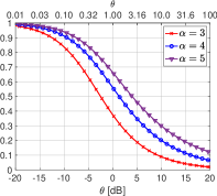
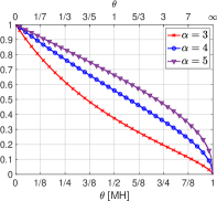
Figure 1: SIR distribution $\bar{F}_{\mathsf{SIR}}(\theta)$ for Poisson networks (per (2) and (3)) with different path loss exponents in units of dB (left) and MH (right). The top axis gives the corresponding values of $\theta$ in standard (linear) units.

I-C Poisson Cellular Network Model

In the following two sections, we focus on the downlink in Poisson cellular networks. We let $\Phi\subset\mathbb{R}^{2}$ be a stationary Poisson point process (PPP) of arbitrary positive intensity and focus on the typical user located at the origin. All our results also hold for the homogeneous independent Poisson (HIP) model, consisting of the union of an arbitrary number of PPPs of arbitrary densities where the base stations of each tier transmit at the same arbitrary power levels.

If $y\in\Phi$ is the desired transmitter, the signal fraction is

$$\mathsf{SF}_{y}=\frac{h_{y}\ell(y)}{\sum_{x\in\Phi}h_{x}\ell(x)}.$$ (1)

We let $\ell(x)=\|x\|^{-\alpha}$, where $\alpha=2/\delta$ is the path loss exponent. $(h_{x})_{x\in\Phi}$ are independent and identically distributed (iid) random variables with $\mathbb{E}(h_{x})=1$ representing fading.

We will study two cases: In Section II, we focus on networks with fading and nearest-base station association, i.e., $\mathsf{SF}=\mathsf{SF}_{y}$ where $y=\operatornamewithlimits{arg\ min}\{x\in\Phi\colon\|x\|\}$. We denote this case by NBA-$m$, where $m$ is the Nakagami-$m$ fading parameter. Section III addresses the no-fading case, or, equivalently, the case of instantaneously-strongest base station association (ISBA) with arbitrary fading. In this case, $\mathsf{SF}=\mathsf{SF}_{y}$ where $y=\operatorname{arg~{}max}\{x\in\Phi\colon h_{x}\ell(x)\}$ or, equivalently, setting all $h_{x}=1$ and selecting $y=\operatornamewithlimits{arg\ min}\{x\in\Phi\colon\|x\|\}$.

II Signal Fraction with Fading and Nearest-Base Station Association

We first focus on Rayleigh fading where the $h_{x}$ are exponential, i.e., NBA-$1$.

II-A Exact Distribution

The SIR distribution is [2]

$$\bar{F}_{\mathsf{SIR}}(\theta)=\frac{1}{\,{}_{2}F_{1}(1,-\delta;1-\delta,-\theta)},$$ (2)

where $\,{}_{2}F_{1}$ is the Gauss hypergeometric function. It follows that the cdf of the $\mathsf{SF}$ is given by $\bar{F}_{\mathsf{SF}}(t)=\bar{F}_{\mathsf{SIR}}(t/(1-t))$, which can be expressed more compactly as

$$\bar{F}_{\mathsf{SF}}(t)=\frac{1}{(1-t)\,_{2}F_{1}(1,1;1-\delta,t)}.$$ (3)

This expression, compared with (2), has the advantage that the last argument of the hypergeometric function does not exceed $1$, which speeds up the evaluation.

II-B Asymptotics and Approximations

II-B1 Rational Approximation

The ccdf of the SF in (3) can be expressed as

$$\bar{F}_{\mathsf{SF}}(t)=\frac{\sum_{n=0}^{\infty}t^{n}}{\sum_{n=0}^{\infty}a_{n}t^{n}},$$

where $a_{n}=\Gamma(n+1)\Gamma(1-\delta)/\Gamma(n+1-\delta)$. Truncations of the infinite series to numerator and denominator polynomials of order $s$ yield simple rational (Padé-type) approximations whose first $s$ derivatives at $t=0$ match those of the exact expression, i.e., they are all asymptotically exact as $t\to 0$. For example, for $s=2$,

$$\bar{F}_{\mathsf{SF}}(t)\sim\frac{1+t+t^{2}}{1+t/(1-\delta)+2t^{2}/((1-\delta)(2-\delta))},\quad t\to 0.$$

II-B2 Polynomial Approximation

The slope of the cdf at $0$ is $f_{\mathsf{SF}}(0)=\mathsf{MISR}$, consistent with the known result $\mathbb{P}(\mathsf{SIR}\leq\theta)\sim\mathsf{MISR}\,\theta$, $\theta\to 0$ [3]. As a result, $\bar{F}_{\mathsf{SF}}(t)\sim 1-\mathsf{MISR}\,t$ is a good approximation for reliabilities of $0.8$ and above (i.e., $t\leq 0.2/\mathsf{MISR}$).

Adding the second-order term, we obtain

$$\bar{F}_{\mathsf{SF}}(t)\sim 1-\mathsf{MISR}\,t+\left(\frac{\mathsf{MISR}^{2}-\delta}{2-\delta}\right)t^{2},\quad t\to 0.$$ (4)

If $\mathsf{MISR}^{2}-\delta>0$, the ccdf is locally convex at $t=0$. This holds if $\delta>(3-\sqrt{5})/2\approx 0.382$ (equivalently, if $\alpha<4/(3-\sqrt{5})\approx 5.24$), and it implies that $1-\mathsf{MISR}\,t$ is a lower bound while (4) is an upper bound. Conversely, for $\delta<0.382$ ($\alpha>5.24$), both first- and second-order asymptotics are upper bounds. We can conclude that in most practical cases, $1-\mathsf{MISR}\,t$ is a lower bound.

Applied to the SIR, we immediately have $F_{\mathsf{SIR}}(\theta)\sim\mathsf{MISR}\,\theta/(1+\theta)$, which is a significantly better approximation than just $\mathsf{MISR}\,\theta$. Generally, $T$ turns polynomials for the SF into rational functions for the SIR of the same order, with improved accuracy. In comparison, the Padé approximation in [4] requires the calculation of twice as many derivatives as the approach via the SF.

Fig. 2 illustrates the exact results and different approximations for the ccdfs of the SF and their application to the ccdfs of the SIR.

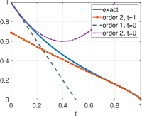
(a) SF, $\alpha=3$.

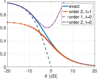
(b) SIR, $\alpha=3$.

(c) SF, $\alpha=4$.

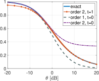
(d) SIR, $\alpha=4$.

Figure 2: SF and SIR ccdfs and approximations for $\alpha=3,4$. The first-order approximation at $t=0$ is $1-\mathsf{MISR}\,t$ and the second-order one is given in (4). The second-order approximation at $t=1$ is given in (5).

II-B3 Series Expansion at $t=1$

From (3) we can derive the second-order series expansion

$$\bar{F}_{\mathsf{SF}}(t)\sim\operatorname{sinc}(\delta)(1-t)^{\delta}(1+\delta(1-t)),\quad t\to 1,$$ (5)

where $\operatorname{sinc}(x)\triangleq\sin(\pi x)/(\pi x)$. It turns out to be a very good approximation for at least $t>2/3$, see Fig. 2. Removing the factor $1+\delta(1-t)$, the first-order expansion is obtained. This asymptotic result shows that the slope at $t=1$ is always infinite, i.e., $f_{\mathsf{SF}}(1)=\infty$.

II-B4 Beta Approximation

For the SIR, there is no simple distribution that closely resembles the entire actual distribution. For the SF, the beta distribution with pdf $f_{\beta}(t)=t^{p-1}(1-t)^{q-1}/{\rm B}(p,q)$, where ${\rm B}$ is the beta function, is a natural candidate. However, merely requiring $f_{\mathsf{SF}}(0)=\mathsf{MISR}$ fixes both parameters, namely $p=1$ and $q=\mathsf{MISR}$, and the resulting $f_{\beta}(t)=\mathsf{MISR}(1-t)^{\mathsf{MISR}-1}$ does not match the asymptotics at $t=1$. For instance, if $\mathsf{MISR}>1$, $f_{\beta}(1)=0$ instead of $\infty$, and for $\mathsf{MISR}=1$, it is just the uniform distribution.

To have more degrees of freedom, we turn to the five-parameter generalized beta distribution put forth in [5]. With a support of $[0,1]$ and $0<f_{\mathsf{SF}}(0)<\infty$, one of the parameters can be eliminated, resulting in the four-parameter pdf

$$f_{{\rm GB}}(t;a,b,p,q)\triangleq\frac{a(1-t^{a})^{q-1}}{b{\rm B}(p,q)(1+(b^{-a}-1)t^{a})^{p+q}},$$

with $a=1/p$. Since $f_{\mathsf{SF}}(0)=\mathsf{MISR}$, we have $b=(\mathsf{MISR}\,p\,{\rm B}(p,q))^{-1}$, which leaves the two parameters $p$ and $q$ to match other statistics.

A simple option is to match the $\Theta((1-t)^{\delta-1})$ asymptotics at $t=1$. It yields $a=p=1$ and $q=\delta$, and thus $b=1-\delta$, resulting in

$$\tilde{f}_{\rm GB}(t)=\frac{\mu}{(1-t)^{1-\delta}(1+\mu t)^{1+\delta}},$$ (6)

where $\mu=\mathsf{MISR}$. It satisfies $\tilde{f}_{\rm GB}(t)\sim\delta(1-\delta)^{\delta}(1-t)^{\delta-1}$, $t\to 1$, which is slightly larger than the actual $\delta\operatorname{sinc}\delta(1-t)^{\delta-1}$ from (5). We call the resulting approximation of the SF and SIR distributions the beta-based simple tight (BEST) approximation. It is formally stated in terms of the ccdfs in the following proposition.

Proposition 1 (BEST approximation)

For Rayleigh fading, the SF and SIR distributions are tightly approximated by

$$\bar{F}_{\mathsf{SF}}^{\small\text{\rm BEST}}(t)=\left(\frac{1-t}{1+\mu t}\right)^{\delta};\;\bar{F}_{\mathsf{SIR}}^{\small\text{\rm BEST}}(\theta)=\big{(}1+(1+\mu)\theta\big{)}^{-\delta},$$ (7)

respectively, where $\mu=\mathsf{MISR}=\delta/(1-\delta)$.

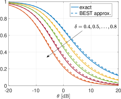
(a) SIR ccdf in dB

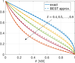
(b) SIR ccdf in MH (or SF ccdf)

Figure 3: SIR ccdfs and BEST approximations (7) for $\delta=0.4,\ldots,0.8$, corresponding to a range of $\alpha$ from $5$ to $2.5$.

Fig. 3 shows the exact SIR ccdfs and the BEST approximations for a range of $\delta$ values. The accuracy of the very simple approximation is remarkable. Its inverse is equally simple, which makes it easy to find the SF or SIR thresholds for a given target reliability.

With a bit more effort we can determine $p$ and $q$ by matching the first and second moments $M_{1}$ and $M_{2}$, given by [5, Eqn. (2.10)]

$$M_{k}=\frac{b^{k}{\rm B}((k+1)p,q)}{{\rm B}(p,q)}\,_{2}F_{1}((k+1)p,kp;(k+1)p+q;1-b^{a}).$$

This way, we obtain

$$\hat{f}_{\rm GB}(t)=f_{\rm GB}\big{(}t;1/p,(\mu p{\rm B}(p,q))^{-1},p,q\big{)}$$ (8)

with $p$ and $q$ chosen such that $M_{1}=\mathbb{E}(\mathsf{SF})$ and $M_{2}=\mathbb{E}(\mathsf{SF}^{2})$. Table I shows the numerically obtained values of $b$, $p$, and $q$ for $\alpha=3,4,5$. The resulting approximations are virtually indistinguishable from the exact distributions.

$$\begin{array}[]{|c|c|c|c|}\hline\cr\delta&b&p&q\\ \hline\cr 2/5&0.7160&0.7385&0.4164\\ 1/2&0.5554&0.8648&0.5276\\ 2/3&0.3598&0.9296&0.7089\\ \hline\cr\end{array}$$

TABLE I: Values of $b$, $p$ and $q$ for different $\delta$ for the generalized beta approximation in (8).

Fig. 4 shows the mean signal fractions for Rayleigh fading, obtained from (3), the BEST approximation (7), a simulation result for the no-fading case (ISBA—see Sec. III), an upper bound for it, and the random base station association scheme discussed in Subsec. III-C.

II-C Other Fading Models

For NBA-$m$, $F_{h}(x)\sim c_{m}x^{m}$, $x\to 0$, where $c_{m}=m^{m-1}/\Gamma(m)$. As shown in [6],

$$\bar{F}_{\mathsf{SIR}}(\theta)\sim 1-c_{m}\theta^{m}\mathbb{E}(\mathsf{ISR}^{m}),\quad\theta\to 0,$$

where $\mathsf{ISR}=I/\mathbb{E}_{h}(S)$ is the interference-to-(average) signal ratio (ISR), i.e., $\mathbb{E}\,\mathsf{ISR}=\mathsf{MISR}$. The $m$-th moment for $m\in\mathbb{N}$ of the ISR for arbitrary fading is given in [6, Thm. 2]. For $m=2$, for example, $\mathbb{E}(\mathsf{ISR}^{2})=2\,\mathsf{MISR}^{2}+\frac{\delta\mathbb{E}(h^{2})}{2-\delta}$. This means that for NBA-$2$, where $c_{2}=2$ and $\mathbb{E}(h^{2})=3/2$,

$$\bar{F}_{\mathsf{SF}}(t)\sim 1-\frac{\delta(3+2\delta-\delta^{2})}{(1-\delta)^{2}(2-\delta)}t^{2},\quad t\to 0.$$

Conversely, the asymptotics as $t\to 1$ do not depend on the fading model, i.e., the tail for NBA-$m$ is $\operatorname{sinc}(\delta)(1-t)^{\delta}$ (see (5)) for any $m>0$ [6, Lemma 6]. Consequently, a beta approximation similar to (6) but with $p=m$ is expected to perform well.

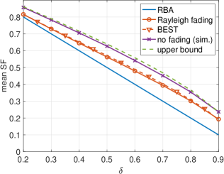
Figure 4: Mean signal fraction for random base station association (RBA) (14), Rayleigh fading (3), the BEST approximation (7), no fading (simulated), and the upper bound (13). The range of $\delta$ corresponds to $\alpha\in[2.25,10]$.

III Signal Fractions Without Fading

III-A The Path Loss Point Process

For a PPP $\Phi\subset\mathbb{R}^{2}$ of intensity $\lambda$, let the path loss point process (PLP) be defined as $\Xi\triangleq\{x\in\Phi\colon\|x\|^{\alpha}/V_{x}\}\subset\mathbb{R}^{+}$, where the $V_{x}$ are iid with $\mathbb{E}(V^{\delta})<\infty$, representing shadowing and/or fading. The PLP is itself Poisson and has the intensity measure $\Lambda([0,r])=\lambda\pi\mathbb{E}(V^{\delta})r^{\delta}$ [1]. Scaling the density does not affect the SF or SIR distributions, so we can equivalently work with a PLP of intensity measure $\Lambda([0,r])=r^{\delta}$, ignoring any shadowing or fading.

If the elements of $\Xi=\{\xi_{1},\xi_{2},\ldots\}$ are ordered (increasingly), their pdfs are [1, Lemma 3]

$$f_{\xi_{k}}(x)=\frac{\delta x^{k\delta-1}}{\Gamma(k)}e^{-x^{\delta}}.$$

In [7], the signal-to-total-received-power ratio process is introduced and shown to be a Poisson-Dirichlet process with parameters $(\delta,0)$. It is defined as $\Psi\triangleq\{\xi\in\Xi\colon\xi^{-1}/P\}\subset[0,1]$, where $P=\sum_{\xi\in\Xi}\xi^{-1}$ is the total received power. The elements of $\Psi=\{\mathsf{SF}_{k}\}_{k\in\mathbb{N}}$, when ordered decreasingly, are the signal fractions when the user is served by the $k$-th strongest base station.

III-B Distribution of Signal Fractions

We first present a lemma summarizing some results on the statistics of the signal fractions.

Lemma 1

For $i\in\mathbb{N}$,

$$\mathbb{E}\left(\frac{\mathsf{SF}_{i}}{\mathsf{SF}_{1}}\right)=\frac{\Gamma(i)\Gamma(1+1/\delta)}{\Gamma(i+1/\delta)},$$ (9)

and

$$\mathbb{E}\log(\mathsf{SF}_{i+1})=\mathbb{E}\log(\mathsf{SF}_{1})-H_{i}/\delta,$$ (10)

where $H_{i}=1+2^{-1}+\ldots+i^{-1}$ is the $i$-th harmonic number. Moreover, letting

$$g_{n}(t)\triangleq\frac{(t^{-1}-1)^{n\delta}}{\Gamma(1+n\delta)(\Gamma(1-\delta))^{n}}$$ (11)

and $\mathsf{SF}_{\Sigma}^{(n)}\triangleq\sum_{i=1}^{n}\mathsf{SF}_{i}$, we have

$$\mathbb{P}(\mathsf{SF}_{n}+t\mathsf{SF}_{\Sigma}^{(n-1)}>t)=g_{n}(t),\quad\tfrac{1}{2}\leq t\leq 1.$$ (12)

Proof:

As shown in [7] the ratio $R_{i}\triangleq\mathsf{SF}_{i+1}/\mathsf{SF}_{i}$ has the cdf

$$\mathbb{P}(R_{i}\leq r)=r^{i\delta},\quad 0\leq r\leq 1,$$

and the $R_{i}$ are independent with $\mathbb{E}(R_{i})=i\delta/(1+i\delta)$. (9) then follows from $\mathsf{SF}_{i}/\mathsf{SF}_{1}=\prod_{k=1}^{i-1}R_{i}$. Similarly, (10) follows from $\mathbb{E}(\log R_{i})=-1/(\delta i)$ and summation.

Lastly, (12) is obtained by rewriting $\mathbb{P}(\xi_{n}^{-1}/\sum_{k=n+1}^{\infty}\xi_{k}^{-1}\geq\theta)$, $\theta\geq 1$, given in [1, Thm. 1], in terms of signal fractions.

∎

Remarks.

• (9) also obtained by integrating the ccdf of $\mathsf{SF}_{i}/\mathsf{SF}_{1}$ given in [2, Lemma 3].

• The expectations in (9) add up to $\mathsf{MISF}=(1-\delta)^{-1}$. This follows from $\sum_{i=1}^{\infty}\mathsf{SF}_{i}/\mathsf{SF}_{1}=1/\mathsf{SF}_{1}$.

• $g_{n}(t)$ in (11) is the ccdf of $\mathsf{SF}_{n}/(1-\mathsf{SF}_{\Sigma}^{(n-1)})$ for $t\geq 1/2$. This is the distribution of $\mathsf{SF}_{n}$ if base stations $1$ to $n-1$ did not exist or, equivalently, if the signals from these base stations were decoded and cancelled through successive interference cancellation [1].

  Some special cases lead to very simple results. For example, setting $t=\delta=1/2$, we have $2/\pi$, $1/\pi$, $4/(3\pi^{2})$, and $1/(2\pi^{2})$ for $n=1,2,3,4$, respectively. For $n=1$, in general, $\bar{F}_{\mathsf{SF}_{1}}(t)=\operatorname{sinc}(\delta)(t^{-1}-1)^{\delta}$, $t\geq 1/2$.

• We can obtain an upper bound on $\mathbb{E}(\mathsf{SF}_{1})$ from the fact that for $t<1/2$, (12) is an upper bound [1]:

  $$\mathbb{E}(\mathsf{SF}_{1})<\int_{0}^{1}\min(1,g_{1}(t))\mathrm{d}t$$ (13)

  This bound, together with a simulation result, is shown in Fig. 4. It is apparent that the bound is rather tight.

• The asymptotic behavior of the cdf of $\mathsf{SF}_{1}$ as $t\to 0$ is $F_{\mathsf{SF}_{1}}(t)\sim e^{s^{\star}(t^{-1}-1)}$ [8, Thm. 1]. Here $s^{\star}$ is given by $\,{}_{1}F_{1}(-\delta,1-\delta,-s^{\star})=s^{\star\delta}\Gamma(-\delta,s^{\star})=0$, where $\Gamma$ is the lower incomplete gamma function. This indicates that the cdf is maximally flat at $t=0$, i.e., all derivatives are $0$.

Fig. 5 shows the ccdfs of $\mathsf{SF}_{1}$ and $\mathsf{SF}_{2}$ for different $\alpha$, partially simulated and partially (for $t\geq 1/2$) given in (11). The support of $\mathsf{SF}_{n}$ is $[0,1/n]$ since the $n$-th largest element cannot exceed $1/n$. Remarkably, the ccdfs of $\mathsf{SF}_{2}$ are insensitive to $\alpha$. At $t=1/8$, they are all about $1/2$. This is explained by the fact that the more dominant $\mathsf{SF}_{1}$, the smaller $\mathsf{SF}_{2}$. Thus the gap between the two ccdfs widens as $\alpha$ increases.

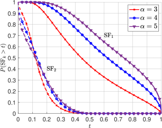
Figure 5: Ccdfs of $\mathsf{SF}_{1}$ and $\mathsf{SF}_{2}$ for $\alpha=3,4,5$. For $t<1/2$, they are obtained by simulation. For $t\geq 1/2$, the ccdfs of $\mathsf{SF}_{1}$ are given by $g_{1}$ in (11) while those of $\mathsf{SF}_{2}$ are $0$.

From [6, Thm. 2], the moments of $\mathsf{SF}_{1}^{-1}=1+\mathsf{ISR}$ are known; the mean is the MISF, and $\operatorname{var}(\mathsf{SF}^{-2})=\delta(2-\delta)^{-1}(1-\delta)^{-2}$. Equipped with the moments, we can derive Markov bounds, such as the lower bound

$$\bar{F}_{\mathsf{SF}}(t)\geq 1-\frac{\delta}{2-\delta}\frac{t^{2}}{(1-\delta-t)^{2}},\quad t<1-\delta.$$

However, these are not particularly tight when applied to the SF.

III-C Random Base Station Association

Here we consider the random base station association scheme (RBA) where, given $\Psi$, the probability of being served by base station $k$ is $\mathsf{SF}_{k}$. The ccdf of the resulting SF, denoted by $\widehat{\mathsf{SF}}$, is

$$\bar{F}_{\widehat{\mathsf{SF}}}(t)=\mathbb{E}\sum_{k=1}^{\infty}\mathsf{SF}_{k}\,\mathbf{1}(\mathsf{SF}_{k}>t).$$

It is shown in [7] that $\widehat{\mathsf{SF}}$ has the (standard) beta pdf

$$f_{\widehat{\mathsf{SF}}}(t)=\frac{\sin(\pi\delta)}{\pi t^{\delta}(1-t)^{1-\delta}}$$ (14)

with mean $1-\delta$, which corresponds to the lower bound in Fig. 4. For $\delta=1/2$, this is the arcsine distribution with cdf $F_{\widehat{\mathsf{SF}}}(t)=2\arcsin\sqrt{t}/\pi$, which has the same $\Theta(\sqrt{t})$ scaling as the cdf for nearest-neighbor association with Nakagami-$1/2$ fading (see Subsec. II-C). It turns out, surprisingly, that the entire distributions appear to match, which leads to the following conjecture.

Conjecture 1

The SF distribution for nearest-base station association with Nakagami-$1/2$ fading (NBA-$\frac{1}{2}$) and $\alpha=4$ is $F_{\mathsf{SF}}(t)=2\arcsin\sqrt{t}/\pi$, $0\leq t\leq 1$.

The evidence supporting the conjecture is that the first $10$ moments of (14) and the empirical moments taken over $2\cdot 10^{7}$ realizations differ by less than $0.03\%$, and the maximum vertical difference between the arcsine cdf and the empirical one is less than $1/3000$.

If the conjecture holds, the mean SF for NBA-$m$ increases from $1-\delta$ for $m=1/2$ to the “no fading” curve in Fig. 4 as $m\to\infty$.

Comparing the cases of RBA, NBA-$1$, and ISBA, we find:

• For RBA: $f_{\mathsf{SF}}(0)=\infty$

• For NBA-$1$: $f_{\mathsf{SF}}(0)=\mathsf{MISR}$

• For ISBA: $f_{\mathsf{SF}}(0)=0$ (and all derivatives are $0$ as well)

The ISBA behavior is consistent with the fact that for NBA-$m$, $m\in\mathbb{N}$, the first $m-2$ derivatives of the pdf are zero at $t=0$. For the tail, $f_{\mathsf{SF}}(t)=\delta\operatorname{sinc}(\delta)(1-t)^{\delta-1}$, $t\to 1$, in all cases.

IV Conclusions

The SIR analysis and/or visualization via signal fractions offers several important advantages:

• Plotting SF distributions (or, equivalently, plotting SIR distributions in MH units) gives the complete information, no truncation is needed. The asymptotics at low and high SIR are directly visible, and $\bar{F}_{\mathsf{SF}}(t)$ near $t=0$ reveals the reliability-rate tradeoff.

• Due to the bounded support of the SF, all integrals (such as the moments) are guaranteed to be finite.

• (Generalized) beta approximations are applicable and may lead to new insights.

• The denominator corresponds to the received (total) signal strength, often abbreviated as RSS. This is the quantity easily measured at a receiver and also the quantity relevant in energy harvesting. Further, it does not change when the desired transmitter (such as the serving base station) changes.

Focusing on Poisson cellular networks, we have found the BEST approximation for Rayleigh fading and offered a conjecture on the SF (and thus SIR) distribution with Nagakami-$1/2$ fading. Both would have been unlikely to be found without the “detour” of using signal fractions.

Lastly, noise can be included by defining the signal fraction with noise (SFN) as $\mathsf{SFN}\triangleq S/(S+N+I)$, where $N$ is the noise power. The mapping from the SINR to the SFN is still given by $T$.

References

- [1] X. Zhang and M. Haenggi, “The Performance of Successive Interference Cancellation in Random Wireless Networks,” IEEE Transactions on Information Theory, vol. 60, pp. 6368–6388, Oct. 2014.
- [2] X. Zhang and M. Haenggi, “A Stochastic Geometry Analysis of Inter-cell Interference Coordination and Intra-cell Diversity,” IEEE Transactions on Wireless Communications, vol. 13, pp. 6655–6669, Dec. 2014.
- [3] M. Haenggi, “The Mean Interference-to-Signal Ratio and its Key Role in Cellular and Amorphous Networks,” IEEE Wireless Communications Letters, vol. 3, pp. 597–600, Dec. 2014.
- [4] H. Nagamatsu, N. Miyoshi, and T. Shirai, “Padé approximation for coverage probability in cellular networks,” in International Workshop on Spatial Stochastic Models for Wireless Networks (SpaSWiN’14), (Hammamet, Tunisia), May 2014.
- [5] J. McDonald and Y. J. Xu, “A generalization of the beta distribution with applications,” Journal of Econometrics, vol. 66, pp. 133–152, 1995.
- [6] R. K. Ganti and M. Haenggi, “Asymptotics and Approximation of the SIR Distribution in General Cellular Networks,” IEEE Transactions on Wireless Communications, vol. 15, pp. 2130–2143, Mar. 2016.
- [7] H.-P. Keeler and B. Blaszczyszyn, “SINR in Wireless Networks and the Two-Parameter Poisson-Dirichlet Process,” IEEE Wireless Communications Letters, vol. 3, pp. 525–528, Oct. 2014.
- [8] R. K. Ganti and M. Haenggi, “SIR Asymptotics in Poisson Cellular Networks without Fading and with Partial Fading,” in IEEE International Conference on Communications (ICC’16), (Kuala Lumpur, Malaysia), May 2016.