Disorder-induced rippled phases and multicriticality in free-standing graphene

Abstract

One of the most exciting phenomena observed in crystalline disordered membranes, including a suspended graphene, is rippling, i.e. a formation of static flexural deformations. Despite an active research, it still remains unclear whether the rippled phase exists in the thermodynamic limit, or it is destroyed by thermal fluctuations. We demonstrate that a sufficiently strong short-range disorder stabilizes ripples, whereas in the case of a weak disorder the thermal flexural fluctuations dominate in the thermodynamic limit. The phase diagram of the disordered suspended graphene contains two separatrices: the crumpling transition line dividing the flat and crumpled phases and the rippling transition line demarking the rippled and clean phases. At the intersection of the separatrices there is the unstable, multicritical point which splits up all four phases. Most remarkably, rippled and clean flat phases are described by a single stable fixed point which belongs to the rippling transition line. Coexistence of two flat phases in the single point is possible due to non-analiticity in corresponding renormalization group equations and reflects non-commutativity of limits of vanishing thermal and rippling fluctuations.

The study of critical elasticity of 2D crystalline membranes dates back to the seminal paper by Nelson and Peliti Nelson1987 , where an idea of crumpling transition (CT), i.e. the transition between flat and crumpled phases, was put forward. A more detailed analysis of the CT and anomalous elasticity of membranes has been developed in Refs. Aronovitz1988 ; Paczuski1988 ; David1988 ; Guitter1988 ; Aronovitz1989 ; Guitter1989 . The interest to the field dramatically increased after discovery of graphene Geim ; Geim1 ; Kim . A suspended graphene (for a review, see Refs. geim07 ; novoselov07 ; graphene-review ; review-DasSarma ; review-Kotov ; book-Katsnelson ; book-Wolf ; book-Roche ) provides an excellent opportunity not only to experimentally verify the existing theoretical predictions for two-dimensional (2D) crystalline membranes but to challenge the theory by new unexpected experimental data. The underlying physics of CT is determined by the thermal out-of-plane fluctuations, so-called flexural phonons (FP). On the one hand, FP tend to crumple the membrane. On the other hand, the long–range interactions between FP, i.e. anharmonic effects, “iron” the membrane and stabilize the flat phase. As a result of such competition, flat and crumpled phases can exist in a clean crystalline membrane.

Along with FP, there can subsist the static, frozen deformations, the so-called ripples, caused by imperfection of the crystal lattice. Such deformations act similarly to FP and also tend to crumple the membrane as was predicted long time ago Morse:1992 ; Nelson_1991 ; Radzihovsky:1991 ; Morse:1992b ; Bensimon_1992 ; Bensimon_1992 . However the physics of disordered membranes with a non-trivial interplay of ripples and thermal fluctuations is much less understood as compared to the clean case. In particular, it is not even fully resolved how many phases exist in such membranes.

The competition between thermal fluctuations and ripples is of crucial importance for free-standing graphene. Indeed, the effect of the thermal fluctuations is controlled by the ratio of temperature $T$ and the bending rigidity $\varkappa_{0}$. In a clean 2D membrane the CT occurs at $T/\varkappa_{0}\sim 1$. In graphene, $\varkappa_{0}\sim 1$ eV, so that the thermal fluctuations alone are not enough to crumple it. At the same time, recent numerical simulations of disordered graphene clearly show the CT Giordanelli2016 . Additional evidence for importance of disorder in graphene is provided by recent experimental measurements of anomalous Hooke’s law (AHL) Nicholl2015 ; Nicholl2017 . Measured scaling exponent was substantially different from the one known from numerical simulations for the clean case Los2016 . These experimental and numerical results imply existence of the rippled phase with properties distinct from the clean one.

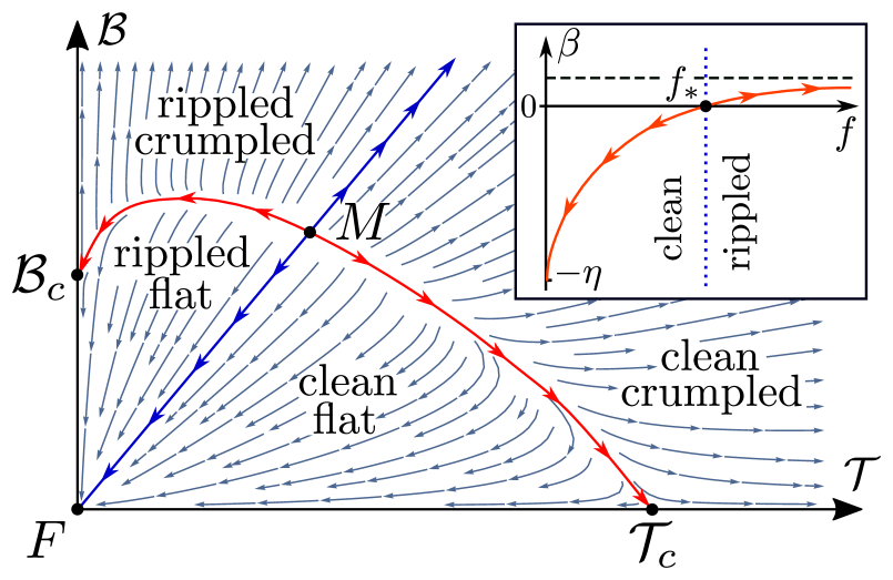
Figure 1: (Color online) Sketch of the phase diagram in plane of the rescaled disorder strength $\mathcal{B}=b/\xi^{2}$ and the amplitude of thermal fluctuations $\mathcal{T}=T/(\varkappa\xi^{2}).$ The solid red curve corresponds to the crumpling transition. The solid blue line is the rippling transition line, separating disordered and clean phases. Fully unstable (multicritical) point is marked by $M$. Two flat phases (clean and disordered) coexists in the stable singular fixed point $F$ reflecting non-commutativity of limits of vanishing thermal and rippling fluctuations. The arrows mark direction of RG flow towards the infrared. Inset: The sketch of a one-parameter RG flow for $f=\mathcal{B}/\mathcal{T}$.

Previous theoretical studies of disordered 2D membranes Morse:1992b ; Bensimon_1992 predict existence of the rippled flat phase at exactly zero temperature, $T=0$, which is unstable with respect to the thermal fluctuations (similar conclusion has been obtained for disordered $D=4-\epsilon$ dimensional membrane Morse:1992 ; Nelson_1991 ; Radzihovsky:1991 ). This conclusion implies absence of the stable rippled phase, and, at first glance, contradicts to observations of Refs. Giordanelli2016 ; Nicholl2015 ; Nicholl2017 ; Los2016 . Recently, the CT in disordered suspended graphene (DSG) was addressed in Ref. Gornyi:2015a . It was shown that disorder can crumple a membrane in agreement with Ref. Giordanelli2016 . It was also found Gornyi:2015a that instability of the rippled phase predicted in Refs. Morse:1992b ; Bensimon_1992 develops logarithmically slow, i.e. the marginal $T=0$ rippled phase controls elastic properties of DSG for $T\neq 0$ in a wide interval of length scales (see also Ref. Doussal2018 ). This marginal behavior can manifest itself in experiments on AHL in graphene Nicholl2015 ; Nicholl2017 as was demonstrated in Ref. Gornyi2017 . However, the rippled phase should not “survive” in the thermodynamic limit even for the case of very strong disorder. Alternatively, observations of Refs. Giordanelli2016 ; Nicholl2015 ; Nicholl2017 can indicate the existence of a stable rippled flat phase at finite temperature. Therefore, a phase diagram of a DSG, when ripples and thermal fluctuations are competed, remains to be still established.

In this Letter, we report the phase diagram of a 2D crystalline membrane with short-ranged curvature disorder (see Fig. 1). Our main results are as follows.

• There are four distinct phases: clean/rippled flat and clean/rippled crumpled ones. There is a fully unstable, multicritical fixed point marked by $M$ that splits up all four phases.

• There is a stable fixed point $F$ corresponding simultaneously to clean and rippled flat phases. Coexistence of two flat phases in the single fixed point reflects non-commutativity of limits of vanishing thermal and rippling fluctuations and is possible due to singularity in corresponding renormalization group (RG) equations, cf. Eq. (8).

• There are two separatrices: one corresponding to the CT (red solid curve) and the other separating clean and rippled phases (blue solid curve).

To obtain this results, we performed a standard $1/d_{c}$ expansion David1988 up to the second order, where $d_{c}$ is the number of FP. As was recently demonstrated Burmistrov2018a ; Burmistrov2018b ; Burmistrov2019a , the second order diagrams contain ones that are not accounted by the so-called Self-Consistent Screening Approximation (SCSA)  Doussal1992 which is frequently discussed as an efficient approximate scheme Gazit2009 ; Doussal2018 . Our results represent first rigorous treatment of anharmonicity in disordered membranes within second-order in $1/d_{\rm c}$ expansion, which is not accounted for neither by SCSA, nor by other approximative schemes such as non-perturbative RG approach Kownacki2009 ; Braghin2010 ; Coquand:2018 . We demonstrate that the finite temperature instability of the rippled phase was an artefact of the first order approximation in $1/d_{\rm c}.$ Our key technical finding is that the terms of higher order in $1/d_{\rm c}$ stabilize the rippled marginal phase and lead to the appearance of the rippling transition (RT) line shown in Fig. 1.

Disorder. —There are many ways to introduce a disorder experimentally: by bombarding graphene with heavy atoms Yeo2018 , by fluorination Daukiya2016 , or by creating macroscopical defects, e.g. artificial holes Yllanes2017 . Theoretically, one classifies disorder with respect to the reflection symmetry related the two opposite sides of a membrane. An example of disorder which preserves the reflection symmetry is the so-called metric or in-plane disorder. It can arise due to the fluctuations in concentration of impurity atoms. Such short-ranged disorder is irrelevant at $T\neq 0$ in the thermodynamic limit, i.e. the clean flat phase is stable against an in-plane disorder Nelson_1991 ; Radzihovsky:1991 ; Gornyi:2015a (for discussion of special case $T=0$, see Ref. Radzihovsky_1992 ). Therefore, we do not consider metric disorder here. Instead, we consider a random curvature disorder proposed in Refs. Morse:1992 ; Morse:1992b ; Bensimon_1992 , which breaks the reflection symmetry. Such disorder naturally arises if impurity atoms are situated on one side of a membrane.

Energy functional. — Membrane’s configuration is parameterized with vector $\bm{r}(\bm{x})\in\mathbb{R}^{d}$, $\bm{x}\in\mathbb{R}^{D}$ where $D=d-d_{c}$. We introduce stretching factor $\xi_{0}$, which characterizes the projective area of a membrane, $\xi_{0}^{2}L^{2}$, and use vectors $\bm{u}(\bm{x})\in\mathbb{R}^{D}$ and $\bm{h}(\bm{x})\in\mathbb{R}^{d_{c}}$ to describe in-plane and out-of-plane displacements: $\bm{r}=\xi_{0}\bm{x}+\bm{u}+\bm{h}$. Although, in the case of graphene $D=2$ and the number of FP is one, we consider $d_{c}$ as an arbitrary parameter which allows us to develop controllable perturbation theory in $1/d_{c}$ David1988 . The energy of crystalline membrane consist of bending and elastic contributions Nelson1987 ; Morse:1992 ; Morse:1992b ; Bensimon_1992

$$\mathcal{F}=\!\int\!d^{2}\bm{x}\left[\frac{\varkappa_{0}}{2}(\Delta\bm{h}-\bm{\beta})^{2}+\mu_{0}u_{\alpha\beta}^{2}+\frac{\lambda_{0}}{2}u_{\alpha\alpha}^{2}\right].$$ (1)

Here $\mu_{0}$ and $\lambda_{0}$ stand for the Lamé coefficients. The last two terms in the right hand side (r.h.s.) of Eq. (1) describe in-plane elastic energy with the strain tensor $u_{\alpha\beta}=(\partial_{\alpha}u_{\beta}+\partial_{\beta}u_{\alpha}+\partial_{\alpha}\bm{h}\partial_{\beta}\bm{h})/2$. Quenched random curvature is added via a zero-mean Gaussian random vector $\bm{\beta}$ Morse:1992 ; Morse:1992b ; Bensimon_1992 . Strength of disorder is controlled by a variance $b_{0}$: $\overline{\beta_{j}(\bm{x})\beta_{k}(\bm{x}^{\prime})}=b_{0}\,\delta_{jk}\delta(\bm{x}-\bm{x}^{\prime})$, $j,k=1,\dots,d_{c}$.

Figure 2: (a) The equation for the screened interaction. The solid line represents the bare Green’s function $\hat{\mathcal{G}}$. The thin dashed line denotes the bare interaction proportional to $Y_{0}$. The dashed line stands for the screened interaction $Y_{q}$. (b) The self-energy correction of the first order in $1/d_{c}$.

Anomalous elasticity. — Although the CT cannot be observed in a clean graphene, the thermal fluctuations around the flat phase lead to highly non-trivial anomalous elastic properties in membranes of size above the so-called Ginzburg length $L_{*}\sim\varkappa_{0}/\sqrt{Y_{0}T}$ Aronovitz1989 . Here $Y_{0}=\frac{4\mu_{0}(\mu_{0}+\lambda_{0})}{(2\mu_{0}+\lambda_{0})}$ denotes the bare (ultraviolet) value of the 2D Young’s modulus. Due to an anharmonic coupling between the in-plane and out-of plane elastic modes the bending rigidity increases in a power law manner for $L\gg L_{*}$ with a certain critical exponent $\eta$: $\varkappa\propto\varkappa_{0}(L/L_{*})^{\eta}$. For graphene $L_{*}\sim 1\div 10$ nm, so that realistic flakes of graphene are in the regime of anomalous elasticity and show a number of highly non-trivial phenomena already verified experimentally, such as mentioned above AHL Guitter1988 ; Aronovitz1989 ; Lopez2015 ; Nicholl2015 ; Los2016 ; Nicholl2017 ; Lopez2017 ; Gornyi2017 , negative thermal expansion coefficient Zakharchenko2009 ; Bao2009 ; Yoom2011 ; Andres2012 ; Silva2014 ; Michel2015 ; Burmistrov2016 , power-law scaling of the phonon-limited conductivity Bolotin2008 ; Castro2010 ; Gornyi2012 , etc.

Crumpling transition. — The scaling equation describing dependence of the stretching factor on a membrane size $L$ reads Gornyi:2015a

$$\frac{d\xi^{2}}{d\ln L}=-\frac{d_{c}}{4\pi}\left({\cal T+B}\right)\xi^{2},\qquad\xi(L_{*})=\xi_{0},$$ (2)

where $\mathcal{T}=T/\varkappa\xi^{2}$ and $\mathcal{B}=b/\xi^{2}$ are rescaled amplitudes of the thermal and disorder–induced fluctuations. The CT occurs when $\xi$ turns into zero at a finite length scale, while in the flat phase $\xi(L\to\infty)>0$. Both the thermal and rippling fluctuations tend to crumple the membrane. In the clean case, $\mathcal{B}=0$, the power law dependence of $\cal{T}$ on $L$ results in the crumpling transition at a very high temperature $T_{c}=4\pi\eta\varkappa_{0}/d_{c}$, which is unreachable for graphene.

In a disordered membrane scaling of ${\cal T}$ and ${\cal B}$ is more intricate than a power law. There is a CT curve in the plane (${\cal T},{\cal B}$) which was found in Ref. Gornyi:2015a by using first order expansion over $1/d_{\rm c}$. Next, we demonstrate that higher order terms in $1/d_{\rm c}$ lead to appearance of the rippling transition line (blue line in Fig. 1).

Replicating fields $\bm{u}$ and $\bm{h}$, integrating over $\bm{u}$ and performing averaging of the replicated partition function over disorder, we obtain the effective free energy Gornyi:2015a .

$$\mathcal{F}_{\rm dis}=\!\sum_{a,b=1}^{N}\int\!\frac{d^{2}\bm{k}}{(2\pi)^{2}}\frac{\hat{\varkappa}_{ab}\,\bm{k}^{4}}{2}\bigl{(}\bm{h}_{\bm{k}}^{(a)}\bm{h}^{(b)}_{-\bm{k}}\bigr{)}+\frac{Y_{0}}{8}\sum_{a=1}^{N}\int\!\frac{d^{2}{\bm{q}}}{(2\pi)^{2}}$$

$$\times\left|\int\frac{d^{2}{\bm{k}}}{(2\pi)^{2}}\frac{[\bm{k}\times\bm{q}]^{2}}{q^{2}}\bigl{(}\bm{h}^{(a)}_{\bm{k}+\bm{q}}\bm{h}^{(a)}_{-\bm{k}}\bigr{)}\right|^{2},$$ (3)

where $\hat{\varkappa}_{ab}=\varkappa_{0}\bigl{[}\delta_{ab}-f_{0}J_{ab}\bigr{]}$ with matrix $\hat{J}$ having all entries equal to one, indices $a,b=1,\dots,N$ enumerate replicas, and $f_{0}=b_{0}\varkappa_{0}/T$.

Anharmonicity of FP result in a renormalization of the parameters of $\mathcal{F}_{\rm dis}$. The necessary information can be extracted from the exact two-point Green’s function $\langle h_{i}^{(a)}(\bm{k})h_{j}^{(b)}(-\bm{k})\rangle\equiv\hat{\bm{\mathcal{G}}}_{ab}(k)\delta_{ij}$ where the average is with respect to the free energy (3). The quadratic part of $\mathcal{F}_{\rm dis}$ determines the bare Green’s function $\hat{\mathcal{G}}_{ab}(k)=T(\delta_{ab}+f_{0}J_{ab})/(\varkappa_{0}k^{4})$. At first, the screening of the interaction between flexural phonons should be taken into account via RPA-type resummation (see Fig. 2). The screened interaction becomes independent of $Y_{0}$ for $q<\sqrt{d_{c}(1+2f_{0})}/L_{*}$ Gornyi:2015a and behaves as $q^{2}/d_{c}$ as $q\to 0$. Using this screened interaction we can construct the regular perturbation theory in $1/d_{c}$ for the self-energy $\hat{\Sigma}$ (see diagrams in Figs. 2 and 3) which relates the exact and bare Green’s functions: $\hat{\bm{\mathcal{G}}}^{-1}=\hat{\mathcal{G}}^{-1}-\hat{\Sigma}$. The perturbation theory for $\hat{\Sigma}(k)$ has infrared logarithmic divergences as $k\to 0$. They can be used to extract the (RG) behavior of the theory.

RG flow. — The corresponding RG equations can be written in the following form.

$$\frac{d\ln\varkappa}{d\ln L}=\eta_{\varkappa}(f),\,\,\frac{d\ln b}{d\ln L}=-\eta_{b}(f),\,\,\frac{d\ln f}{d\ln L}=\beta(f),$$ (4)

where $f=b\varkappa/T=\mathcal{B}/\mathcal{T}$ and $\eta_{b}(f)=\eta_{\varkappa}(f)-\beta(f)$. We emphasize that RG equation for $f$ decouples, while $\varkappa$ and $b$ are slave variables. The RG functions can be expanded as $\eta_{\varkappa/b}={\eta_{\varkappa/b}^{(1)}}/{d_{c}}+{\eta_{\varkappa/b}^{(2)}}/{d_{c}^{2}}+\dots$ and $\beta={\beta^{(1)}}/{d_{c}}+{\beta^{(2)}}/{d_{c}^{2}}+\dots$. The first order coefficients are $\beta_{1}=-2(1+3f)/(1+2f)^{2}$ and $\eta_{\varkappa}^{(1)}=2(1+3f+f^{2})/(1+2f)^{2}$ Morse:1992b ; Gornyi:2015a . Our explicit calculations in the second order in $1/d_{c}$ yield See Supplemental Material

$$\beta^{(2)}= -\Bigl{[}73+803f+3667f^{2}+8517f^{3}+9278f^{4}$$

$$+ 3420f^{5}+186f^{6}-68\zeta(3)\bigl{(}1+11f+49f^{2}$$

$$+ 111f^{3}+128f^{4}+58f^{5}+6f^{6}\bigr{)}\Bigr{]}\Bigl{/}\bigl{[}27(1+2f)^{6}\bigr{]},$$

$$\eta_{\varkappa}^{(2)}= \Bigl{[}73+803f+3550f^{2}+7743f^{3}+7995f^{4}+3046f^{5}$$

$$+ 265f^{6}-68\zeta(3)\bigl{(}1+11f+49f^{2}+111f^{3}+129f^{4}$$

$$+ 64f^{5}+9f^{6}\bigr{)}\Bigr{]}\Bigl{/}\bigl{[}27(1+2f)^{6}\bigr{]}.$$ (5)

The functions $\beta^{(2)}$ and $\eta_{\varkappa}^{(2)}$ have finite limit at $f\to\infty$. The RG flow for $f$ has three fixed points: $0$, $\infty$, and $f_{*}\approx 8.5\,d_{c}$ (see the inset to Fig. 1) footnote . At the fixed point $f=0$ which is stable in the infrared the bending rigidity and disorder variance acquires the power law scaling, $\varkappa\sim L^{\eta}$, $b\sim L^{-\eta^{\prime}}$ where Burmistrov2019a

$$\eta=\eta^{\prime}/2=\eta_{\varkappa}(0)\approx 2/d_{c}-[68\zeta(3)-73]/(27d_{c}^{2}).$$ (6)

The other infrared stable fixed point is located at $f=\infty$. We note that within the first order in $1/d_{c}$ this fixed point is marginally unstable Morse:1992b . At $f=\infty$ the bending rigidity and the disorder variance has also power-law scaling with momentum, $\varkappa\sim L^{\eta_{\infty}}$, $b\sim L^{-\eta^{\prime}_{\infty}}$ where

$$\eta_{\infty}\approx\frac{1}{2d_{c}}-\frac{612\zeta(3)-265}{1728d_{c}^{2}},\,\eta^{\prime}_{\infty}\approx\eta_{\infty}-\frac{68\zeta(3)-31}{228d_{c}^{2}}.$$ (7)

The fixed point at $f=f_{*}$ is unstable in the infrared and is characterized by the exponent of divergent correlation length $\nu=1/[fd\beta/df]|_{f=f_{*}}=288d_{c}^{2}/[68\zeta(3)-31]$ Comment-Mohana .

Figure 3: Diagrams for the self-energy corrections in the second order in $1/d_{c}$. Diagrams (a) and (b) are included in SCSA. Diagrams (c)-(f) are not taken into account by SCSA.

From Eqs. (2) and (4) we find the RG equations governing the flow of parameters $\mathcal{T}$ and $\mathcal{B}$.

$$\begin{split}\frac{d\ln{\cal T}}{d\ln L}&=\frac{d_{c}}{4\pi}({\cal B}+{\cal T})-\eta_{\varkappa}({\cal B}/{\cal T}),\\ \frac{d\ln{\cal B}}{d\ln L}&=\frac{d_{c}}{4\pi}({\cal B}+{\cal T})-\eta_{b}({\cal B}/{\cal T}).\end{split}$$ (8)

The corresponding flow diagram is shown in Fig. 1. There is the unstable fixed point at ${\cal T}_{c}=4\pi\eta/d_{c}$ and ${\cal B}=0$, corresponding to the CT due to thermal fluctuations in the absence of disorder. This fixed point controls the transition between the clean flat phase and the clean crumpled phase. The unstable fixed point at ${\cal T}$ and ${\cal B}_{c}=4\pi\eta^{\prime}_{\infty}/d_{c}$ corresponds to the disorder-driven CT Gornyi:2015a . This fixed point controls transition between flat and crumpled rippled phases. Remarkably, both the clean flat phase ($f=0$) and the rippled flat phase ($f=\infty$) are described by the single singular infrared stable fixed point $F$ at ${\cal T}={\cal B}=0.$ The singularity at ${\cal T}\to 0$ and ${\cal B}\to 0$ is clearly seen if one uses in Eq. (8), the explicit expressions for the functions $\eta_{\varkappa}({\cal B}/{\cal T})$ and $\eta_{b}({\cal B}/{\cal T})$. Eqs. (8) admit the multicritical fixed point $M$ at ${\cal T}_{*}=4\pi\eta_{\varkappa}(f_{*})/[d_{c}(1+f_{*})]$ and ${\cal B}_{*}=f_{*}{\cal T}_{*}$ (see Fig. 1). This multifractal fixed point has two unstable directions: along the CT curve, which demarks flat and crumpled phases, and along the RT line, ${\cal B}=f_{*}{\cal T},$ which splits up clean and rippled phases and connects $M$ and $F$. The scaling along these two separatrices are controlled by the critical exponents $\nu$ and $1/\eta_{\varkappa}(f_{*}),$ respectively. We emphasise the striking resemblance of our RG flow diagram with the one for the random bond Ising model Nishimori . The RT line corresponds to the so-called Nishimori line LeDoussal1988 .

Discussion and conclusion. — Our key result is the demonstration of the ripples stabilization by sufficiently strong disorder. More precisely, two transitions occur with increasing the disorder at fixed other parameters. For ${\cal T}<{\cal T}_{*}$ (see Fig. 1), the first transition corresponds to the stabilization of ripples, while the second one is the CT. On the contrary, for ${\cal T}>{\cal T}_{*},$ the CT happens before the stabilization of ripples. Our phase diagram suggests also a possibility of the RT with decreasing temperature at the fixed disorder. As a very interesting subject for further research, we expect that the phase diagram is even reacher in the case of long-ranged disorder LD&R1993 .

In the course of derivation of RG Eqs. (8) we neglected the term $\partial_{\alpha}\bm{u}\partial_{\beta}\bm{u}$ in the expression for the strain tensor $u_{\alpha\beta}$. It can be shown Future that this approximation is justified for $\mathcal{B},\mathcal{T}\ll 1$. The terms $\partial_{\alpha}\bm{u}\partial_{\beta}\bm{u}$ provide additional contributions to Eqs. (8) that are of higher order in powers of $\mathcal{B}$ and $\mathcal{T}$. These terms do not affect the properties of the fixed point F but can result in corrections of higher order in $1/d_{c}$ to the position of the CT line as well as to the critical exponents governing scaling behavior at the fixed points $\mathcal{B}_{c}$, $\mathcal{T}_{c}$, and M Future .

The relevance of our theory for realistic graphene membranes is supported by the numerical simulations Giordanelli2016 where the CT with increase of disorder was clearly seen and the fractal dimension of the crumpled membrane was reported. A detailed comparison of our theory with Ref. Giordanelli2016 is however not possible due to a lack of simulations at various temperatures.

To conclude, we predict existence of two disorder-dominated rippled phase (flat and crumpled) in a disordered crystalline membrane with a short-range disorder. By using fully controlled standard $1/d_{c}$ expansion, we derive coupled RG equations for the bending rigidity and disorder strength and establish the phase diagram of a generic crystalline membrane (see Fig. 1). We demonstrate existence of the multicritical point (M), the singular stable point (F), where the rippled flat and clean flat phases coexist, and the rippling transition line connecting these two fixed points.

ONLINE SUPPORTING INFORMATION
Disorder-induced rippled phases and multicriticality in a free-standing graphene

In this Supplementary Material we present derivation of the RG equations (4) of the main text.

I Self-energy correction

The interaction between flexural phonons modifies the Green’s function. The exact Green’s function can be written as follows (in the replica limit $N\to 0$):

$$\hat{\bm{\mathcal{G}}}(k)=T\Bigl{[}\varkappa(1-f\hat{J})k^{4}-\hat{\Sigma}(k)\Bigr{]}^{-1}.$$ (9)

As well-known, before constructing the perturbation theory in the interaction between flexural phonons it is important to take into account screening of this interaction by the flexural phonon themselves. This screening (see Fig. 2b of the main text) is determined by the bare polarization operator

$$\hat{\Pi}_{ab}(q)=\frac{d_{c}}{3T}\int_{k}\frac{[\bm{k\times q}]^{4}}{q^{4}}\hat{\mathcal{G}}_{ab}(|\bm{k-q}|)\hat{\mathcal{G}}_{ab}(k)=\Bigl{(}1+2f+f^{2}\hat{J}\Bigr{)}\frac{d_{c}T}{16\pi\varkappa^{2}q^{2}}.$$ (10)

Here we introduced for a brevity the following shorthand notation: $\int_{k}\equiv\int d^{2}\bm{k}/(2\pi)^{2}$. Summation of the geometric series shown in Fig. 2b of the main text yields the screened interaction

$$\hat{N}(q)=\frac{\hat{Y}_{q}}{2}=\frac{Y_{0}/2}{1+3Y_{0}\hat{\Pi}(q)/2}=\frac{Y_{0}}{2}\frac{q^{2}}{q^{2}+\tilde{q}_{*}^{2}}\left(1-\frac{f^{2}\hat{J}}{1+2f}+\frac{q^{2}}{q^{2}+\tilde{q}_{*}^{2}}\frac{f^{2}\hat{J}}{1+2f}\right).$$ (11)

We mention that the screened interaction at small momenta,

$$q\ll\tilde{q}_{*}=\sqrt{1+2f_{0}}/L_{*}$$

becomes independent of the Young modulus $Y_{0}$ and proportional to $1/d_{c}$.

I.1 Contribution of the first order in $1/d_{c}$

The self-energy correction of the first order in $1/d_{c}$ is given by the diagram in Fig. 2a of the main text. It can be written as:

$$\begin{aligned} \hat{\Sigma}^{(1)}_{ab}(k)&=-2\int_{q}\frac{[\bm{k\times q}]^{4}}{q^{4}}\hat{N}_{ab}(q)\hat{\mathcal{G}}_{ab}(|\bm{k-q}|)\\ &=-\frac{2}{d_{c}}\varkappa k^{4}\Biggl{[}\frac{1+3f+f^{2}-f^{3}\hat{J}}{(1+2f)^{2}}L_{0}\left(\frac{k}{\tilde{q}_{*}}\right)+\frac{f^{2}(1+f\hat{J})}{(1+2f)^{2}}L_{1}\left(\frac{k}{\tilde{q}_{*}}\right)\Biggr{]}_{ab}\end{aligned}$$ (12)

where

$$L_{m}(K)=\int_{0}^{\infty}\frac{dq}{q}\frac{q^{2m}\min\bigl{\{}{q^{4}}/{K^{4}},1\bigr{\}}}{(1+q^{2})^{m+1}}.$$ (13)

For $m=0,1$ they are given explicitly as follows

$$L_{0}(K)=-\ln K+\frac{1}{2}\ln(1+K^{2})+\frac{K^{2}-\ln(1+K^{2})}{2K^{4}},\quad L_{1}(K)=\frac{K^{2}-\ln(1+K^{2})}{K^{4}}.$$ (14)

In the limit $k/\tilde{q}_{*}\ll 1$ and $N\to 0$, we find

$$\hat{\Sigma}^{(1)}(k)=-\frac{2}{d_{c}}\varkappa k^{4}\bigl{(}\alpha_{1}\ln\frac{q_{*}}{k}-f\gamma_{1}\hat{J}\ln\frac{q_{*}^{\prime}}{k}\bigr{)},$$ (15)

where $q_{*}=\tilde{q}_{*}\exp[1/4+\gamma_{1}/(2\alpha_{1})]$ and $q_{*}^{\prime}=\tilde{q}_{*}\exp(-1/4)$ and

$$\alpha_{1}=\frac{1+3f+f^{2}}{(1+2f)^{2}},\quad\gamma_{1}=\frac{f^{2}}{(1+2f)^{2}}.$$ (16)

I.2 Contribution of the second order in $1/d_{c}$

In this subsection we present results for the contribution of the second order in $1/d_{c}$ to the self-energy (see diagrams in Fig. 3 of the main text)

I.2.1 Diagram Fig. 3a

The corresponding contribution to the self-energy has the following form

$$\hat{\Sigma}^{(2,a)}_{ab}(k)=-\frac{2}{T}\int_{q}\Bigl{[}\hat{\mathcal{G}}(|\bm{k-q}|)\Sigma^{(1)}(|\bm{k-q}|)\hat{\mathcal{G}}(|\bm{k-q}|)\Bigr{]}_{ab}\frac{[\bm{k\times q}]^{4}}{q^{4}}\hat{N}_{ab}(q).$$ (17)

Computing the integrals over momentum $q$ in the same way as in Ref. S (1), we obtain for $k/\tilde{q}_{*}\ll 1$ and $N\to 0$:

$$\hat{\Sigma}^{(2,a)}(k)=\frac{2}{d_{c}^{2}}\varkappa k^{4}\Biggl{\{}\alpha^{(a)}\Bigl{[}\ln^{2}\frac{q_{*}}{k}+\frac{1}{2}\ln\frac{q_{*}}{k}\Bigr{]}-f\gamma^{(a)}\hat{J}\Bigl{[}\ln^{2}\frac{q_{*}^{\prime}}{k}+\frac{1}{2}\ln\frac{q_{*}^{\prime}}{k}\Bigr{]}+\tilde{\alpha}^{(a)}\ln\frac{q_{*}}{k}-f\tilde{\gamma}^{(a)}\hat{J}\ln\frac{q_{*}^{\prime}}{k}\Biggr{\}},$$ (18)

where

$$\alpha^{(a)} =\frac{1+7f+16f^{2}+12f^{3}+f^{4}}{(1+2f)^{4}},\quad\gamma^{(a)}=\frac{f^{2}(2+6f+f^{2})}{(1+2f)^{4}},$$

$$\tilde{\alpha}^{(a)} =-\frac{c\gamma_{1}}{\beta_{1}}\beta^{(2,a)}+\frac{f^{2}(1+5f+5f^{2})}{(1+2f)^{4}},\quad\tilde{\gamma}^{(a)}={\gamma}^{(2,a)}+\frac{3f^{4}}{(1+2f)^{4}}.$$ (19)

I.2.2 Diagram Fig. 3b

The diagram can be considered as the first order correction to the self-energy in which the interaction line is changed due to correction to the polarization operator:

$$\hat{\Sigma}^{(2,b)}_{ab}(k)=\!\frac{6}{T}\!\!\int_{q}\!\frac{[\bm{k\times q}]^{4}}{q^{4}}\Bigl{[}\hat{N}(q)\delta\hat{\Pi}(q)\hat{N}(q)\Bigr{]}_{ab}\!\hat{\mathcal{G}}_{ab}(|\bm{k-q}|),$$

$$\delta\hat{\Pi}_{cd}(q)=\frac{2d_{c}}{3T^{2}}\int_{k}\frac{[\bm{k\times q}]^{4}}{q^{4}}\hat{\mathcal{G}}_{cd}(|\bm{k-q}|)\Bigl{[}\hat{\mathcal{G}}(k)\hat{\Sigma}^{(1)}(k)\hat{\mathcal{G}}(k)\Bigr{]}_{cd}.$$ (20)

The correction to the polarization operator can be computed as follows:

$$\delta\hat{\Pi}(q)=-\frac{T\delta\hat{\pi}(q/\tilde{q}_{*})}{4\pi\varkappa^{2}q^{2}},\quad\delta\hat{\pi}(q)=\sum_{j=0,1}\delta\hat{\pi}_{j}\tilde{L}_{j}(q),$$ (21)

where

$$\delta\hat{\pi}_{0}=\frac{1+6f+10f^{2}+2f^{3}+f^{2}(2+6f+f^{2})\hat{J}}{(1+2f)^{2}},\quad\delta\hat{\pi}_{1}=\frac{f^{2}(1+4f+3f^{2}\hat{J})}{(1+2f)^{2}},$$ (22)

and

$$\tilde{L}_{m}(q)=\int_{0}^{1}dkkL_{m}(kq)+\int_{1}^{\infty}\frac{dk}{k^{3}}L_{m}(kq).$$ (23)

The functions $\tilde{L}_{0}$ and $\tilde{L}_{1}$ can be computed exactly as follows

$$\tilde{L}_{0}(q)=\frac{(1+q^{2})}{6q^{2}}\Bigl{[}\frac{(1+q^{2})^{2}}{q^{2}}\ln(1+q^{2})-1\Bigr{]}-\frac{q^{2}+3}{3}\ln q,$$

$$\tilde{L}_{1}(q)=\frac{q^{2}}{3}\ln q-\frac{(q^{2}-2)}{6q^{2}}\Bigl{[}\frac{(1+q^{2})^{2}}{q^{2}}\ln(1+q^{2})-1\Bigr{]}.$$ (24)

Substituting the expression (21) for the correction to the polarization operator into Eq. (20), we obtain in the limits $k/\tilde{q}_{*}\ll 1$ and $N\to 0$:

$$\hat{\Sigma}^{(2,b)}(k)=-\frac{4}{d_{c}^{2}}\varkappa k^{4}\Biggl{\{}\alpha^{(b)}\Bigl{[}\ln^{2}\frac{q_{*}}{k}+\frac{1}{2}\ln\frac{q_{*}}{k}\Bigr{]}-f\gamma^{(b)}\hat{J}\Bigl{[}\ln^{2}\frac{q_{*}^{\prime}}{k}+\frac{1}{2}\ln\frac{q_{*}^{\prime}}{k}\Bigr{]}+\tilde{\alpha}^{(b)}\ln\frac{q_{*}}{k}-f\tilde{\gamma}^{(b)}\hat{J}\ln\frac{q_{*}^{\prime}}{k}\Biggr{\}}$$ (25)

where

$$\alpha^{(b)} =\frac{1+9f+30f^{2}+42f^{3}+19f^{4}+2f^{5}}{(1+2f)^{5}},\quad\gamma^{(b)}=\frac{f^{3}(2+7f+2f^{2})}{(1+2f)^{5}},$$

$$\tilde{\alpha}^{(b)} =-\frac{c\gamma_{1}}{\beta}\beta^{(b)}+\frac{f^{2}(1+7f+15f^{2}+6f^{3})}{(1+2f)^{5}},\quad\tilde{\gamma}^{(b)}=\gamma^{(b)}-c\frac{f^{4}(1-2f)}{(1+2f)^{5}}.$$ (26)

I.2.3 Diagram Fig. 3c

The correction to the self-energy shown in Fig. 3c of the main text can be written as follows

$$\hat{\Sigma}^{(2,c)}_{ab}(k)=\frac{4}{T}\int_{q,Q}\frac{[\bm{k\times q}]^{2}}{q^{2}}\frac{[\bm{k\times Q}]^{2}}{q^{2}}\frac{[\bm{(k-q)\times Q}]^{2}}{Q^{2}}\frac{[\bm{(k-Q)\times q}]^{2}}{q^{2}}\hat{\mathcal{G}}_{ac}(|\bm{k-q}|)\hat{\mathcal{G}}_{cd}(|\bm{k-Q}|)$$

$$\times\hat{\mathcal{G}}_{db}(|\bm{k-q-Q}|)\hat{N}_{ad}(q)\hat{N}_{cb}(Q).$$ (27)

Taking the integrals over momenta in the same way as in Ref. S (1), we find in the limits $k/\tilde{q}_{*}\ll 1$ and $N\to 0$:

$$\hat{\Sigma}^{(2,c)}(k)=\frac{7}{3d_{c}^{2}}\varkappa k^{4}\bigl{(}\alpha^{(c)}-f\gamma^{(c)}\hat{J}\bigr{)}\ln\frac{q_{*}}{k},$$ (28)

where

$$\alpha^{(c)}=\frac{1+7f+17f^{2}+16f^{3}+5f^{4}}{(1+2f)^{4}},\quad\gamma^{(c)}=\frac{f^{2}(1+4f+f^{2})}{(1+2f)^{4}}.$$ (29)

I.2.4 Diagram Fig. 3d

The correction to the self-energy shown in Fig. 3d of the main text can be written as follows

$$\hat{\Sigma}^{(2,d)}_{ab}(k)=-\frac{4d_{c}}{T^{2}}\int_{Q,p,p^{\prime}}\frac{[\bm{p\times Q}]^{2}}{Q^{2}}\frac{[\bm{p^{\prime}\times Q}]^{2}}{Q^{2}}\frac{[\bm{p\times p^{\prime}}]^{2}}{|\bm{p-p^{\prime}}|^{2}}\frac{[\bm{k\times(p-p^{\prime})}]^{4}}{|\bm{p-p^{\prime}}|^{4}}\frac{[\bm{(p-Q)\times(p^{\prime}-Q)}]^{2}}{|\bm{p-p^{\prime}}|^{2}}\hat{N}_{lm}(Q)$$

$$\times\hat{N}_{ac}(|\bm{p-p^{\prime}}|)\hat{N}_{bd}(|\bm{p-p^{\prime}}|)\hat{\mathcal{G}}_{cl}(p)\hat{\mathcal{G}}_{dl}(|\bm{p-Q}|)\hat{\mathcal{G}}_{cm}(p^{\prime})\hat{\mathcal{G}}_{dm}(|\bm{p^{\prime}-Q}|)\hat{\mathcal{G}}_{ab}(|\bm{k-p+p^{\prime}}|).$$ (30)

Integration over momenta can be performed in the same way as in Ref. S (1). Then for $k/\tilde{q}_{*}\ll 1$ and $N\to 0$ we retrieve:

$$\hat{\Sigma}^{(2,d)}(k)=-\frac{2}{d_{c}^{2}}\varkappa k^{4}\bigl{(}\alpha^{(d)}-f\gamma^{(d)}\hat{J}\bigr{)}\ln\frac{q_{*}}{k},$$ (31)

where

$$\alpha^{(d)}=\frac{1+11f+49f^{2}+111f^{3}+130f^{4}+72f^{5}+16f^{6}}{(1+2f)^{6}},\quad\gamma^{(d)}=\frac{2f^{4}}{(1+2f)^{5}}.$$ (32)

I.2.5 Diagram Fig. 3e

The correction to the self-energy shown in Fig. 3e of the main text is as follows

$$\hat{\Sigma}^{(2,e)}_{ab}(k)=-\frac{8d_{c}}{T^{2}}\int_{q,p,Q}\frac{[\bm{k\times q}]^{2}}{q^{2}}\frac{[\bm{k\times Q}]^{2}}{Q^{2}}\frac{[\bm{p\times q}]^{2}}{q^{2}}\frac{[\bm{(k-q)\times(Q-q)}]^{2}}{|\bm{q-Q}|^{2}}\frac{[\bm{(p-Q)\times(p-q)}]^{2}}{|\bm{q-Q}|^{2}}$$

$$\times\frac{[\bm{p\times Q}]^{2}}{Q^{2}}\hat{N}_{ac}(q)\hat{N}_{bd}(Q)\hat{N}_{lm}(|\bm{q-Q}|)\hat{\mathcal{G}}_{cd}(p)\hat{\mathcal{G}}_{am}(|\bm{k-q}|)\hat{\mathcal{G}}_{mb}(|\bm{k-Q}|)\hat{\mathcal{G}}_{cl}(|\bm{p-q}|)\hat{\mathcal{G}}_{dl}(|\bm{p-Q}|).$$ (33)

Integration over momenta can be performed in the same way as in Ref. S (1). Then we obtain for $k/\tilde{q}_{*}\ll 1$ and $N\to 0$:

$$\hat{\Sigma}^{(2,e)}(k)=-\frac{58}{27d_{c}^{2}}\varkappa k^{4}\bigl{(}\alpha^{(e)}-f\gamma^{(e)}\hat{J}\bigr{)}\ln\frac{q_{*}}{k},$$ (34)

where

$$\alpha^{(e)}=\frac{1+11f+49f^{2}+111f^{3}+129f^{4}+67f^{5}+10f^{6}}{(1+2f)^{6}},\quad\gamma^{(e)}=\frac{2f^{4}(2+5f+2f^{2})}{(1+2f)^{6}}.$$ (35)

I.2.6 Diagram Fig. 3f

The correction to the self-energy shown in Fig. 3f of the main text is given by the following explicit expression:

$$\hat{\Sigma}^{(2,f)}_{ab}(k)=\frac{8d^{2}_{c}}{T^{3}}\int_{p,p^{\prime},q,Q}\frac{[\bm{k\times q}]^{4}}{q^{4}}\frac{[\bm{p\times q}]^{2}}{q^{2}}\frac{[\bm{p\times Q}]^{2}}{Q^{2}}\frac{[\bm{(p-Q)\times(q-Q)}]^{2}}{|\bm{q-Q}|^{2}}\frac{[\bm{(p^{\prime}-Q)\times(q-Q)}]^{2}}{|\bm{q-Q}|^{2}}$$

$$\times\frac{[\bm{p^{\prime}\times Q}]^{2}}{Q^{2}}\frac{[\bm{p^{\prime}\times q}]^{2}}{q^{2}}\hat{N}_{ac}(q)\hat{N}_{bd}(q)\hat{N}_{st}(|\bm{q-Q}|)\hat{N}_{lm}(Q)\hat{\mathcal{G}}_{cl}(p)\hat{\mathcal{G}}_{cs}(|\bm{p-Q}|)\hat{\mathcal{G}}_{ls}(|\bm{p-q}|)\hat{\mathcal{G}}_{dm}(p^{\prime})$$

$$\times\hat{\mathcal{G}}_{dt}(|\bm{p^{\prime}-Q}|)\hat{\mathcal{G}}_{mt}(|\bm{p^{\prime}-q}|)\hat{\mathcal{G}}_{ab}(|\bm{k-q}|).$$ (36)

Integrating over momenta in the same way as in Ref. S (1), and taking the limits $k/\tilde{q}_{*}\ll 1$ and $N\to 0$, we obtain:

$$\hat{\Sigma}^{(2,f)}_{ab}(k)=\frac{3+68\zeta(3)}{27d_{c}^{2}}\varkappa k^{4}\bigl{(}\alpha^{(f)}-f\gamma^{(f)}\hat{J}\bigr{)}\ln\frac{q_{*}}{k},$$ (37)

where

$$\alpha^{(f)}=\frac{1+11f+49f^{2}+111f^{3}+129f^{4}+64f^{5}+9f^{6}}{(1+2f)^{6}},\quad\gamma^{(f)}=\frac{f^{4}(1+6f+3f^{2})}{(1+2f)^{6}}.$$ (38)

I.2.7 Contribution of the second order in $1/d_{c}$

All in all, the six diagrams in Fig. 3 of the main text yield the following contribution to the self-energy in the second order in $1/d_{c}$:

$$\hat{\Sigma}^{(2)}(k)=-\frac{\alpha_{2}+2\tilde{\alpha}_{2}}{d_{c}^{2}}\ln\frac{q_{*}}{k}-\frac{2\alpha_{2}^{\prime}}{d_{c}^{2}}\ln^{2}\frac{q_{*}}{k}+f\hat{J}\Biggl{[}\frac{\gamma_{2}+2\tilde{\gamma}_{2}}{d_{c}^{2}}\ln\frac{q_{*}^{\prime}}{k}+\frac{2\gamma_{2}^{\prime}}{d_{c}^{2}}\ln^{2}\frac{q_{*}^{\prime}}{k}\Biggr{]},$$ (39)

where

$$\alpha_{2}^{\prime}=2\alpha^{(b)}-\alpha^{(a)},\quad\tilde{\alpha}_{2}=2\tilde{\alpha}^{(b)}-\tilde{\alpha}^{(a)},\quad\gamma_{2}^{\prime}=2\gamma^{(b)}-\gamma^{(a)},\quad\tilde{\gamma}_{2}=2\tilde{\gamma}^{(b)}-\tilde{\gamma}^{(a)}.$$ (40)

and

$$\alpha_{2} =\alpha_{2}^{\prime}-\frac{7}{3}\alpha^{(c)}+2\alpha^{(d)}+\frac{58}{27}\alpha^{(e)}-\frac{3+68\zeta(3)}{27}\alpha^{(f)},$$

$$\gamma_{2} =\gamma_{2}^{\prime}-\frac{7}{3}\gamma^{(c)}+2\gamma^{(d)}+\frac{58}{27}\gamma^{(e)}-\frac{3+68\zeta(3)}{27}\gamma^{(f)}.$$ (41)

II RG equations

II.1 First order in $1/d_{c}$

The effect of the first order correction (15) to the self-energy can be interpreted as $1/d_{c}$ corrections to $\varkappa$ and $f$:

$$\varkappa(k)=\varkappa\left[1+\frac{2\alpha_{1}}{d_{c}}\ln\frac{q_{*}}{k}\right],\quad\varkappa(k)f(k)=\varkappa f\left[1+\frac{2\gamma_{1}}{d_{c}}\ln\frac{q_{*}^{\prime}}{k}\right],\quad f(k)=f\left[1+\frac{2(\gamma_{1}-\alpha_{1})}{d_{c}}\ln\frac{q_{*}^{\prime\prime}}{k}\right],$$ (42)

where $q_{*}^{\prime\prime}=q_{*}e^{1/4+c\gamma_{1}/(\alpha_{1}-\gamma_{1})}$. We mention that the perturbative results (42) suggest that the bare parameters $\varkappa$ and $f$ coincide with the renormalized parameters at the scales $q_{*}$ and $q_{*}^{\prime\prime}$, respectively, i.e. $\varkappa\equiv\varkappa(q_{*})$ and $f\equiv f(q_{*}^{\prime\prime})$. Also we note that the following relation holds $\varkappa(q_{*})f(q_{*}^{\prime\prime})=\varkappa(q_{*}^{\prime})f(q_{*}^{\prime})$.

The perturbative corrections (42) can be recast in the form of the RG equations S (1, 1):

$$-\frac{d\ln\varkappa}{d\ln k}=\frac{\eta_{\varkappa}^{(1)}}{d_{c}},\qquad-\frac{d\ln f}{d\ln k}=\frac{\beta^{(1)}}{d_{c}},\qquad\qquad\eta_{\varkappa}^{(1)}=2\alpha_{1},\qquad\beta^{(1)}=2(\gamma_{1}-\alpha_{1}).$$ (43)

Since the momentum scale are arranged as $q_{*}^{\prime}<q_{*}<q_{*}^{\prime\prime}$, strictly speaking, the RG equations (43) are valid for $k<q_{*}^{\prime}$.

II.2 Second order in $1/d_{c}$

The results (15) and (39) for the self-energy allows us to write the following perturbative expansions for bending rigidity $\varkappa$ and the parameter $f$:

$$\frac{\varkappa(k)}{\varkappa(q_{*})}= 1+\frac{2\alpha_{1}}{d_{c}}\ln\frac{q_{*}}{k}+\frac{1}{d_{c}^{2}}\Bigl{(}\alpha_{2}+4f\gamma_{1}\frac{d\alpha_{1}}{df}\ln\frac{q_{*}^{\prime}}{q_{*}}\Bigr{)}\ln\frac{q_{*}}{k}+\frac{2}{d_{c}^{2}}\Bigl{(}\alpha_{1}^{2}+(\gamma_{1}-\alpha_{1})f\frac{d\alpha_{1}}{df}\Bigr{)}\ln^{2}\frac{q_{*}}{k}$$ (44)

$$\frac{f(k)}{f(q_{*}^{\prime\prime})}= 1+\left(\frac{2(\gamma_{1}-\alpha_{1})}{d_{c}}+\frac{(\gamma_{2}-\alpha_{2})}{d_{c}^{2}}\right)\ln\frac{q_{*}^{\prime\prime}}{k}+\frac{2(\gamma_{1}-\alpha_{1})}{d_{c}^{2}}\frac{d[f(\gamma_{1}-\alpha_{1})]}{df}\ln^{2}\frac{q_{*}^{\prime\prime}}{k}.$$ (45)

We emphasize that $f$ in the right hand side (r.h.s.) of Eqs. (44) and (45) is defined at the momentum scale $q_{*}^{\prime\prime}$. Also we note that in derivation of Eqs. (44) and (45) we used the following non-trivial relations:

$$\alpha_{2}^{\prime}=\alpha_{1}^{2}+(\gamma_{1}-\alpha_{1})f\frac{d\alpha_{1}}{df},\quad\gamma_{2}^{\prime}=\gamma_{1}^{2}+(\gamma_{1}-\alpha_{1})f\frac{d\gamma_{1}}{df}.$$ (46)

The perturbative expansion (45) describes how the disorder parameter $f$ transforms under a change of the momentum scale from $q_{*}^{\prime\prime}$ to $k$. The form of Eq. (44) is a bit unconventional since its r.h.s. involves $f$ at not at the momentum scale $q_{*}$ but at another momentum scale, $q_{*}^{\prime\prime}$. Therefore it is convenient to rewrite Eq. (44) with $f$ defined at the momentum scale $q_{*}$ in its r.h.s.:

$$\frac{\varkappa(k)}{\varkappa(q_{*})}=1+\left(\frac{2\alpha_{1}}{d_{c}}+\frac{\alpha_{2}}{d_{c}^{2}}\right)\ln\frac{q_{*}}{k}+\frac{2}{d_{c}^{2}}\Bigl{(}\alpha_{1}^{2}+(\gamma_{1}-\alpha_{1})f\frac{d\alpha_{1}}{df}\Bigr{)}\ln^{2}\frac{q_{*}}{k}.$$ (47)

We stress that $f$ in the r.h.s. of Eq. (47) is defined at the momentum scale $q_{*}$.

The results (45) and (47) can be cast from perturbative solutions of the following RG equations for $\varkappa$ and $f$:

$$-\frac{d\ln\varkappa}{d\ln k}=\frac{\eta_{\varkappa}^{(1)}}{d_{c}}+\frac{\eta_{\varkappa}^{(2)}}{d_{c}^{2}},\qquad-\frac{d\ln f}{d\ln k}=\frac{\beta^{(1)}}{d_{c}}+\frac{\beta^{(2)}}{d_{c}^{2}},\qquad\qquad\eta_{\varkappa}^{(2)}=\alpha_{2},\qquad\beta^{(2)}=\alpha_{2}-\gamma_{2}.$$ (48)

RG equations (48) equivalent to Eqs. (4) of the main text.

References

• (1) D. Nelson and L. Peliti, Fluctuations in membranes with crystalline and hexatic order, J. Phys., 48, 1085 (1987).
• (2) J. A. Aronovitz and T. C. Lubensky, Fluctuations of solid membranes, Phys. Rev. Lett. 60, 2634 (1988).
• (3) M. Paczuski, M. Kardar, and D. R. Nelson, Landau theory of the crumpling transition, Phys. Rev. Lett.60, 2638 (1988).
• (4) F. David and E. Guitter, Europhys. Lett. (EPL), Crumpling transition in elastic membranes: Renormalization group treatment, 5, 709 (1988).
• (5) E. Guitter, F. David, S. Leibler, and L. Peliti, Crumpling and buckling transitions in polymerized membranes, Phys. Rev. Lett. 61, 2949 (1988).
• (6) J. Aronovitz, L. Golubovic, and T. C. Lubensky, Fluctuations and lower critical dimensions of crystalline membranes, J. Phys. 50, 609 (1989).
• (7) E. Guitter, F. David, S. Leibler, and L. Peliti, Thermodynamical behavior of polymerized membranes, J. Phys. 50, 1787 (1989).
• (8) K. S. Novoselov, A. K. Geim, S. V. Morozov, D. Jiang, Y. Zhang, S. V. Dubonos, I. V. Grigorieva, and A. A. Firsov, Electric field effect in atomically thin carbon films, Science 306, 666 (2004).
• (9) K. S. Novoselov, A. K. Geim, S. V. Morozov, D. Jiang, M. I. Katsnelson, I. V. Grigorieva, S. V. Dubonos, and A. A. Firsov, Two-dimensional gas of massless Dirac fermions in graphene, Nature 438, 197 (2005).
• (10) Y. Zhang, Y.-W. Tan, H. L. Stormer, and P. Kim, Experimental observation of the quantum Hall effect and Berry’s phase in graphene, Nature 438, 201 (2005).
• (11) A. K. Geim and K. S. Novoselov, The rise of graphene, Nature Materials 6, 183 (2007).
• (12) K. S. Novoselov, Z. Jiang, Y. Zhang, S. V. Morozov, H. L. Stormer, U. Zeitler, J. C. Maan, G. S. Boebinger, P. Kim, and A. K. Geim, Room-temperature quantum Hall effect in Graphene, Science 315, 1379 (2007).
• (13) A. H. Castro Neto, F. Guinea, N. M. R. Peres, K. S. Novoselov, and A. K. Geim, The electronic properties of graphene, Rev. Mod. Phys. 81, 109 (2009).
• (14) S. Das Sarma, S. Adam, E. H. Hwang, and E. Rossi, Electronic transport in two-dimensional graphene, Rev. Mod. Phys. 83, 407 (2011).
• (15) V. N. Kotov, B. Uchoa, V. M. Pereira, F. Guinea, and A. H. Castro Neto, Electron-electron interactions in graphene: Current status and perspectives, Rev. Mod. Phys. 84, 1067 (2012).
• (16) M. I. Katsnelson, Graphene: Carbon in Two Dimensions, Cambridge University Press (2012).
• (17) E. L. Wolf, Graphene: A New Paradigm in Condensed Matter and Device Physics, Oxford University Press (2014).
• (18) L. E. F. Foa Torres, S. Roche, J.-C. Charlier, Introduction to Graphene-Based Nanomaterials From Electronic Structure to Quantum Transport, Cambridge University Press (2014).
• (19) D. C. Morse, T. C. Lubensky, and G. S. Grest, Quenched disorder in tethered membranes, Phys. Rev. A 45, R2151 (1992).
• (20) D. R. Nelson and L. Radzihovsky, Polymerized membranes with quenched random internal disorder, Europhys. Letters (EPL) 16, 79 (1991).
• (21) L. Radzihovsky and D. R. Nelson, Statistical mechanics of randomly polymerized membranes, Phys. Rev. A 44, 3525 (1991).
• (22) D. C. Morse and T. C. Lubensky, Curvature disorder in tethered membranes: A new flat phase at T=0, Phys. Rev. A 46, 1751 (1992).
• (23) D. Bensimon, D. Mukamel, and L. Peliti, Quenched curvature disorder in polymerized membranes, Europhys. Letters (EPL) 18, 269 (1992).
• (24) I. Giordanelli, M. Mendoza, J. S. Andrade Jr., M. A. F. Gomes, and H. J. Herrmann, Crumpling damaged graphene, Scientific Reports, 6, 25891 (2016).
• (25) R. J. T. Nicholl, H. J. Conley, N. V. Lavrik, I. Vlassiouk, Y. S. Puzyrev, V. P. Sreenivas, S. T. Pantelides, and K. I. Bolotin, The effect of intrinsic crumpling on the mechanics of free-standing graphene, Nat. Comm. 6, 8789 (2015).
• (26) R. J. T. Nicholl, N. V. Lavrik, I. Vlassiouk, B. R. Srijanto, and K. I. Bolotin, Hidden area and mechanical nonlinearities in freestanding graphene, Phys. Rev. Lett. 118, 266101 (2017).
• (27) J. H. Los, A. Fasolino, and M. I. Katsnelson, Scaling behavior and strain dependence of in–plane elastic properties of graphene, Phys. Rev. Lett. 116, 015901 (2016).
• (28) I. V. Gornyi, V. Y. Kachorovskii, and A. D. Mirlin, Rippling and crumpling in disordered free-standing graphene, Phys. Rev. B 92, 155428 (2015).
• (29) P. Le Doussal and L. Radzihovsky, Anomalous elasticity, fluctuations and disorder in elastic membranes, Ann. Phys. (N.Y.) 392, 340 (2018).
• (30) I. V. Gornyi, V. Yu. Kachorovskii, and A. D. Mirlin, Anomalous Hooke’s law in disordered graphene, 2D Mater. 4, 011003 (2017).
• (31) I. S. Burmistrov, I. V. Gornyi, V. Y. Kachorovskii, M. I. Katsnelson, J. H. Los, and A. D. Mirlin, Stress-controlled Poisson ratio of a crystalline membrane: Application to graphene, Phys. Rev. B 97, 125402 (2018).
• (32) I. S. Burmistrov, V. Y. Kachorovskii, I. V. Gornyi, and A. D. Mirlin, Differential Poisson’s ratio of a crystalline two-dimensional membrane, Ann. Phys. (N.Y.) 396, 119 (2018).
• (33) D. R. Saykin, I. V. Gornyi, V. Y. Kachorovskii, and I. S. Burmistrov, Absolute Poisson’s ratio and the bending rigidity exponent of a crystalline two-dimensional membrane, arXiv:2002.04554.
• (34) P. Le Doussal and L. Radzihovsky, Self-consistent theory of polymerized membranes, Phys. Rev. Lett. 69, 1209 (1992).
• (35) D. Gazit, Structure of physical crystalline membranes within the self-consistent screening approximation, Phys. Rev. E 80, 041117 (2009).
• (36) J.-P. Kownacki and D. Mouhanna, Crumpling transition and flat phase of polymerized phantom membranes, Phys. Rev. E 79, 040101 (2009).
• (37) F. L. Braghin and N. Hasselmann, Thermal fluctuations of free-standing graphene, Phys. Rev. B 82, 035407 (2010).
• (38) O. Coquand, K. Essafi, J.-P. Kownacki, and D. Mouhanna, Glassy phase in quenched disordered crystalline membranes, Phys. Rev. E 97, 030102(R) (2018).
• (39) S. Yeo, J. Han, S. Bae, D. Su Lee, Coherence in defect evolution data for the ion beam irradiated graphene, Scientific Reports 8, 13973 (2018).
• (40) H. Li, L. Daukiya, S. Haldar, A. Lindblad, B. Sanyal, O. Eriksson, D. Aubel, S. Hajjar-Garreau, L. Simon, and K. Leifer, Site-selective local fluorination of graphene induced by focused ion beam irradiation, Scientific Reports, 6, 19719 (2016).
• (41) D. Yllanes, S. S. Bhabesh, D. R. Nelson, and M. J. Bowick, Thermal crumpling of perforated two-dimensional sheets, Nat. Comm. 8, 1381 (2017).
• (42) L. Radzihovsky and P. Le Doussal, Crumpled glass phase of randomly polymerized membranes in the large d limit, J. Phys. I 2, 599 (1992).
• (43) G. Lopez-Polin, C. Gomez-Navarro, V. Parente, F. Guinea, M. I. Katsnelson, F. Perez-Murano, and J. Gomez-Herrero, Increasing the elastic modulus of graphene by controlled defect creation, Nat. Phys. 11, 26 (2015).
• (44) G. Lopez- Polin, M. Jaafar, F. Guinea, R. Roldan, C. Gomez- Navarro, and J. Gomez-Herrero, The influence of strain on the elastic constants of graphene, Carbon 124, 42, (2017).
• (45) K. V. Zakharchenko, M. I. Katsnelson, and A. Fasolino, Finite temperature lattice properties of graphene beyond the quasiharmonic approximation, Phys. Rev. Lett. 102, 046808 (2009).
• (46) W. Bao, F. Miao, Z. Chen, H. Zhang, W. Jang, C. Dames, and C. N. Lau, Controlled ripple texturing of suspended graphene and ultrathin graphite membranes, Nat. Nanotech. 4, 562 (2009).
• (47) D. Yoon, Y.-W. Son, and H. Cheong, Negative thermal expansion coefficient of graphene measured by Raman spectroscopy, Nano Lett. 11, 3227 (2011).
• (48) P. L. de Andres, F. Guinea, and M. I. Katsnelson, Bending modes, anharmonic effects, and thermal expansion coefficient in single-layer and multilayer graphene, Phys. Rev. B 86, 144103 (2012).
• (49) A. L. C. da Silva, Ladir Cândido, J. N. Teixeira Rabelo, G.-Q. Hai, and F. M. Peeters, Anharmonic effects on thermodynamic properties of a graphene monolayer, Europhys. Lett. (EPL), 107, 56004 (2014).
• (50) K. H. Michel, S. Costamagna, and F. M. Peeters, Theory of anharmonic phonons in two-dimensional crystals, Phys. Rev. B 91, 134302 (2015).
• (51) I. S. Burmistrov, I. V. Gornyi, V. Y. Kachorovskii, M. I. Katsnelson, A. D. Mirlin, Quantum elasticity of graphene: Thermal expansion coefficient and specific heat, Phys. Rev. B 94, 195430 (2016).
• (52) K. I. Bolotin, K. J. Sikes, J. Hone, H. L. Stormer, and P. Kim, Temperature-dependent transport in suspended graphene, Phys. Rev. Lett. 101, 096802 (2008).
• (53) E. V. Castro, H. Ochoa, M. I. Katsnelson, R. V. Gorbachev, D. C. Elias, K. S. Novoselov, A. K. Geim, and F. Guinea, Limits on charge carrier mobility in suspended graphene due to flexural phonons, Phys. Rev. Lett.105, 266601 (2010).
• (54) I. V. Gornyi, V. Yu. Kachorovskii, and A. D. Mirlin, Conductivity of suspended graphene at the Dirac point, Phys. Rev. B 86, 165413 (2012).
• (55) Will be published elsewhere.
• (56) See Supplemental Material.
• (57) We note that analysis of the structure of the higher order in $1/d_{c}$ diagrams suggests that the corrections to the position of the unstable fixed point are $O(1/d_{c})$ and, thus, are negligible at $d_{c}\gg 1$.
• (58) Recently, the unstable fixed point similar to $f_{*}$ has been found for a disordered membrane of $D=4-\epsilon$ dimension within the second order expansion in $\epsilon$ and for a 2D disordered membrane within analytically uncontrolled NPRG approach Coquand:2018 .
• (59) H. Nishimori, Statistical Physics of Spin Glasses and Information Processing. An Introduction, Clarendon Press, Oxford (2001).
• (60) P. Le Doussal, A. Brooks Harris, Location of the Ising Spin-Glass Multicritical Point on Nishimori’s Line, Phys. Rev. Lett. 61, 625 (1988).
• (61) P. Le Doussal and L. Radzihovsky, Flat glassy phases and wrinkling of polymerized membranes with long-range disorder, Phys. Rev. B 48, 3548 (1993).

References

• (1)
• S (1) D. R. Saykin, I. V. Gornyi, V. Y. Kachorovskii, and I. S. Burmistrov, arXiv:2002.04554.
• S (1) D. C. Morse and T. C. Lubensky, Phys. Rev. A 46, 1751 (1992).
• S (1) I. V. Gornyi, V. Y. Kachorovskii, and A. D. Mirlin, Phys. Rev. B 92, 155428 (2015).