A Discrete-Time, Time-Delayed Lur’e Model
with Biased Self-Excited Oscillations

Abstract

Self-excited systems arise in many applications, such as biochemical systems, mechanical systems with fluid-structure interaction, and fuel-driven systems with combustion dynamics. This paper presents a Lur’e model that exhibits biased self-excited oscillations under constant inputs. The model involves asymptotically stable linear dynamics, time delay, a washout filter, and a saturation nonlinearity. For all sufficiently large scalings of the loop transfer function, these components cause divergence under small signal levels and decay under large signal amplitudes, thus producing an oscillatory response. A bias-generation mechanism is used to specify the mean of the oscillation. The main contribution of the paper is a detailed analysis of a discrete-time version of this model.

1 Introduction

A self-excited system has the property that the input is constant but the response is oscillatory. Self-excited systems arise in numerous applications, such as biochemical systems, fluid-structure interaction, and combustion. The classical example of a self-excited system is the van der Pol oscillator, which has two states whose asymptotic response converges to a limit cycle. A self-excited system, however, may have an arbitrary number of states and need not possess a limit cycle. Overviews of self-excited systems are given in [1, 2], and applications to chemical and biochemical systems are discussed in [3, 4, 5]. Self-excited thermoacoustic oscillation in combustors is discussed in [6, 7, 8]. Self-excited oscillations of a tropical ocean-atmosphere system are discussed in [9]. Fluid-structure interaction and its role in aircraft wing flutter is discussed in [10, 11, 12, 13]. Wind-induced self-excited motion and its role in the Tacoma Bridge collapse is discussed in [14].

Models of self-excited systems are typically derived in terms of the relevant physics of the application. From a systems perspective, the main interest is in understanding the features of the components of the system that give rise to self-sustained oscillations. Understanding these mechanisms can illuminate the relevant physics in specific domains and provide unity across various domains.

A unifying model for self-excited systems is a feedback loop involving linear and nonlinear elements; systems of this type are called Lur’e systems. Lur’e systems have been widely studied in the classical literature on stability theory [15]. Within the context of self-excited systems, Lur’e systems under various assumptions are considered in [2, 16, 17, 18, 19, 20, 21, 22, 23, 24]. Application to thermoacoustic oscillation in combustors is considered in [25]. Self-oscillating discrete-time systems are considered in [26, 27, 28, 29].

Roughly speaking, self-excited oscillations arise from a combination of stabilizing and destabilizing effects. Destabilization at small signal levels causes the response to grow from the vicinity of an equilibrium, whereas stabilization at large signal levels causes the response to decay from large signal levels. In particular, negative damping at low signal levels and positive damping at high signal levels is the mechanism that gives rise to a limit cycle in the van der Pol oscillator [30, pp. 103–107]. Note that, although systems with limit-cycle oscillations are self-excited, the converse need not be true since the response of a self-excited system may oscillate without the trajectory reaching a limit cycle. Alternative mechanisms exist, however; for example, time delays are destabilizing, and Lur’e models with time delay have been extensively considered as models of self-excited systems [31].

The present paper considers a time-delayed Lur’e (TDL) model that exhibits self-excited oscillations. This model, which is illustrated in Figure 1, incorporates the following components:

1. Asymptotically stable linear dynamics.

2. Time delay.

3. A washout (that is, highpass) filter.

4. A continuous, bounded nonlinearity ${\mathcal{N}}\colon{\mathbb{R}}\to{\mathbb{R}}$ that satisfies ${\mathcal{N}}(0)=0$, is either nondecreasing or nonincreasing, and changes sign (positive to negative or vice versa) at the origin.

5. A bias-generation mechanism, which produces an offset in the oscillatory response that depends on the value of the constant external input.

A notable feature of this model is that self-oscillations are guaranteed to exist for asymptotically stable dynamics that are not necessarily passive as in [32]. We note that washout filters are used in [33] to achieve stabilization, whereas, in the present paper, they are used to create self-oscillations.

Figure 1: Continuous-time, time-delayed Lur’e model with constant input $u$ and bias generation.

For this time-delay Lur’e model, the time-delay provides the destabilization mechanism, while, under large signal levels, the saturation function yields a constant signal, which effectively breaks the loop, thus allowing the open-loop dynamics to stabilize the response. This stabilization occurs at large amplitude. In order to create an oscillatory response, the Lur’e model includes a washout filter, which removes the DC component of the delayed signal $y_{\rm d}$ and allows the saturation function to operate in its small-signal linear region. A similar feature appears in [16, 17, 18, 2, 19] in the form of the numerator $s$ in $G$ for the case where $y$ represents velocity. This combination of elements produces self-excited oscillations for all sufficiently large scalings of the asymptotically stable dynamics. An additional feature of this model is the ability to produce oscillations with a bias, that is, an offset. This is done by the bias-generation mechanism involving the scalar $\beta.$ Example 1.1 illustrates the response of the model in Figure 1.

Example 1.1

Let $G(s)=\frac{1}{s+1},$ $W(s)=\frac{s}{0.001s+1},$ and ${\mathcal{N}}(y_{\rm f})=\tfrac{5}{2}\tanh(\tfrac{2}{5}y_{\rm f}).$ For $T_{\rm d}=5$ s, $\beta=5,$ and $v=10,$ the response of the TDL model is shown in Figure 2. In particular, the output $y(t)$ converges to a periodic signal with bias $v\beta G(0)=50.$ Next, the effect of $v,$ $\beta,$ and $T_{\rm d}$ on the oscillatory response of the model will be shown. The response of the TDL model for $v=2.5,5,$ $\beta=5,$ and $T_{\rm d}=1,2$ s is shown in Figure 3, while the response for $v=2.5,$ $\beta=5,10,$ and $T_{\rm d}=1,2$ s is shown in Figure 4. Note that, for the same transfer function $G$, different values of $v,$ $\beta,$ and $T_{\rm d}$ produce different waveforms for $y(t)$ and different phase portraits of $y_{\rm f}(t)$ versus $y(t).$ $\diamond$

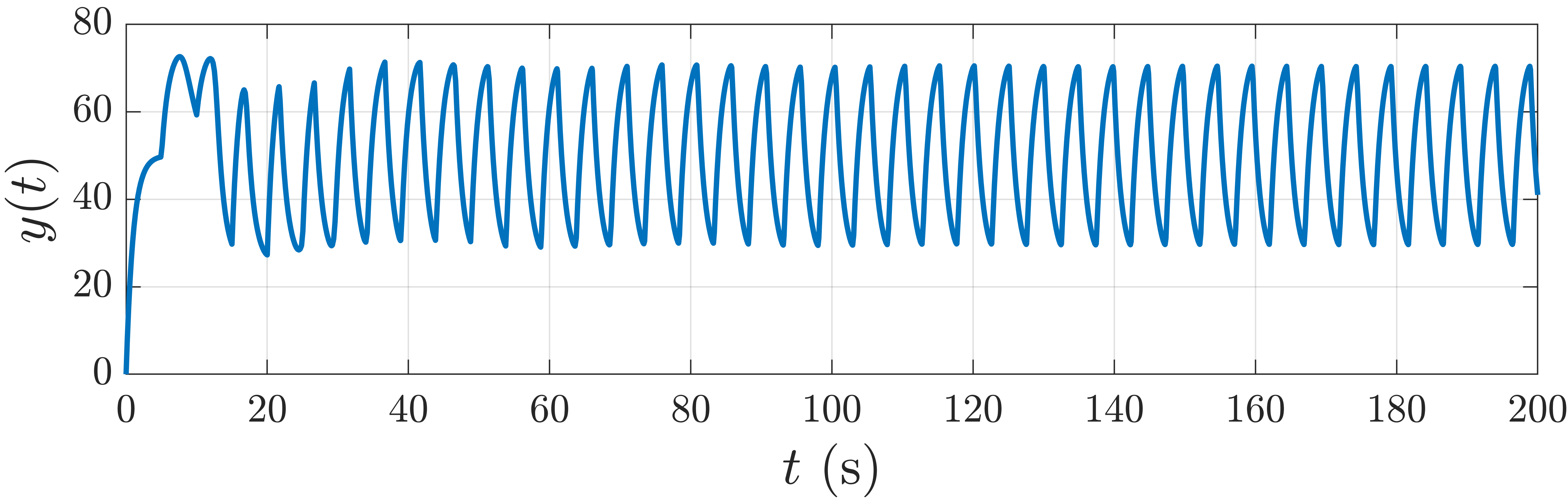
Figure 2: Example 1.1 Self-excited oscillatory response of the continuous-time time-delay Lur’e model shown in Figure 1. Note that the oscillation has nonzero bias due to the bias-generation mechanism.

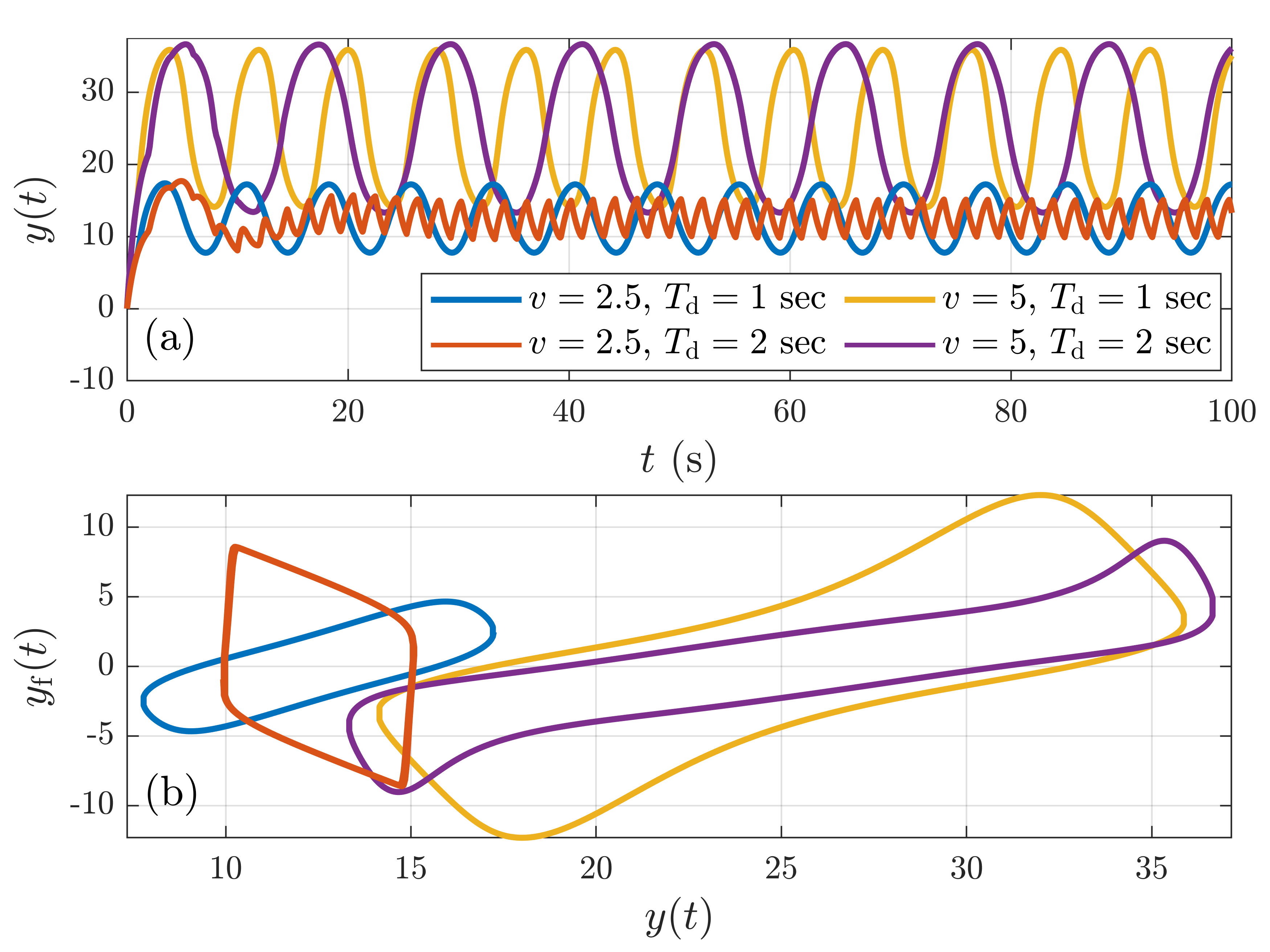
Figure 3: Example 1.1: For $v=2.5,5,$ $\beta=5,$ and $T_{d}=1,2$ s, (a) shows the response $y(t),$ and (b) shows $y(t)$ versus $y_{{\rm f}}(t)$ for $t>100$ s. Note that the shapes of the oscillations are distinct for different parameters under the same linear dynamics given by $G.$

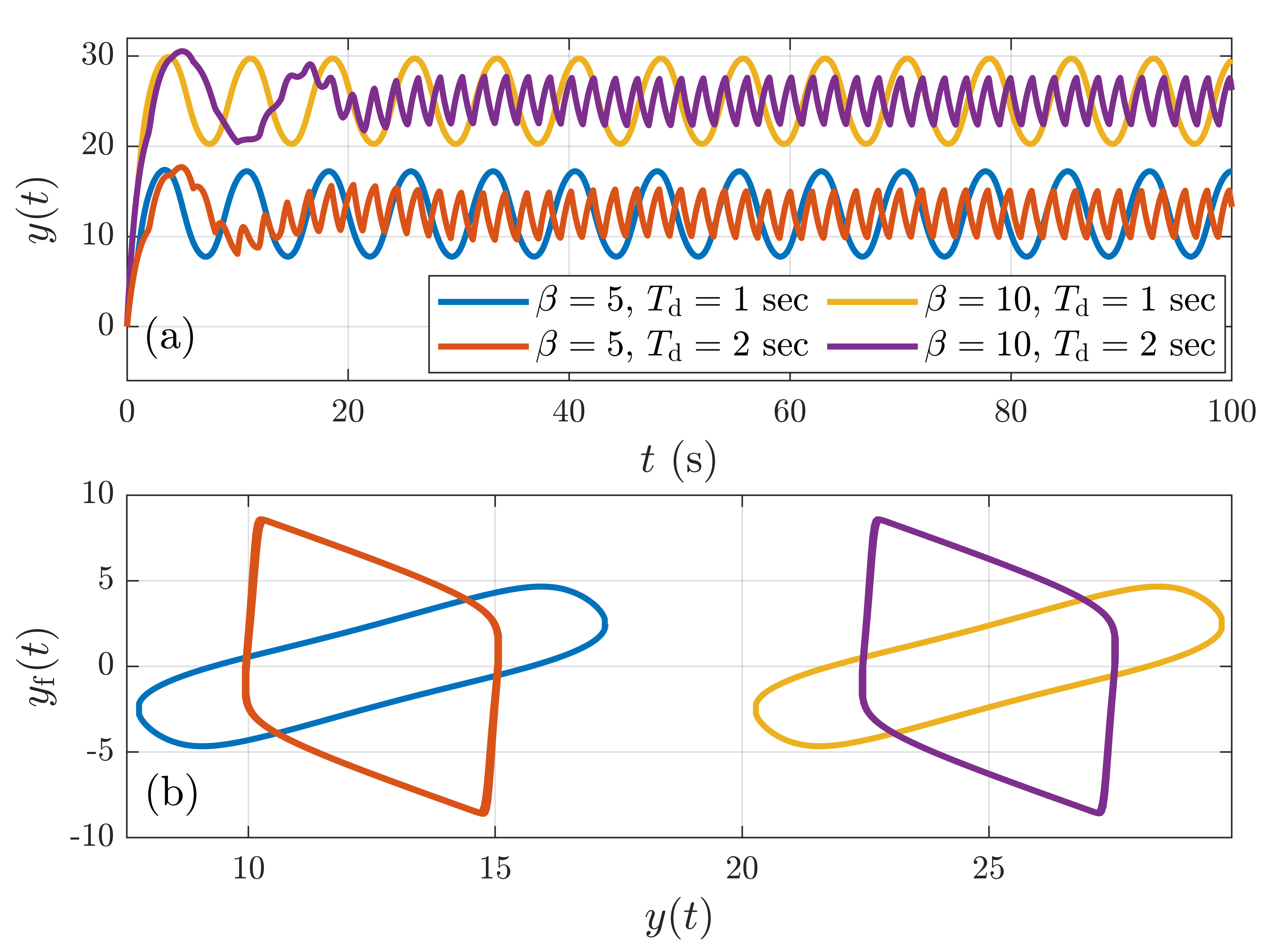
Figure 4: Example 1.1: For $v=2.5,$ $\beta=5,10,$ and $T_{d}=1,2$ s, (a) shows the response $y(t),$ and (b) shows $y(t)$ versus $y_{{\rm f}}(t)$ for $t>100$ s. Note the effect of the value of $\beta$ on the output offset and how the shape of the oscillation is kept for different values of $\beta.$

The analysis and examples in the paper focus on a discrete-time version of the time-delayed Lur’e model with the standard saturation function. This setting simplifies the analysis of solutions as well as the numerical simulations.

The contents of the paper are as follows. Section II considers a discrete-time linear feedback model and analyzes the range of values of $\alpha$ for which the closed-loop model is asymptotically stable. Section III extends the problem in Section II by including a saturation nonlinearity. This discrete-time Lur’e model is shown to have an asymptotically oscillatory response for sufficiently large values of the loop gain. Section IV extends the Lur’e model to include a bias-generation mechanism.

Preliminary results relating to the present paper appear in [34]. Key differences between [34] and the present paper include the following: 1) Lemma 2.1 and v) of Theorem 2.2 are not given in [34]; 2) due to limited space, no proofs are given in [34]; and 3) the present paper includes several examples that do not appear in [34].

Define ${\mathbb{Z}}\stackrel{{\scriptstyle\triangle}}{{=}}\{\ldots,-1,0,1,\ldots\},$ ${\mathbb{N}}\stackrel{{\scriptstyle\triangle}}{{=}}\{0,1,2,\ldots\},$ and ${\mathbb{P}}\stackrel{{\scriptstyle\triangle}}{{=}}\{1,2,\ldots\}.$ For all polynomials $p,$ ${\rm spr}(p)$ denotes the maximum magnitude of all elements of $\operatorname{roots}(p).$ For all nonzero $z=x+\jmath y\in{\mathbb{C}}$, where $x$ and $y$ are real, $\arg z=\operatorname{atan2}(y,x)\in(-\pi,\pi]$ denotes the principal angle of $z$. Let $P\stackrel{{\scriptstyle\triangle}}{{=}}N/D$ be a transfer function with no zeros on the unit circle, where $N$ and $D$ are coprime, $m\stackrel{{\scriptstyle\triangle}}{{=}}{\rm deg}N$ and $n\stackrel{{\scriptstyle\triangle}}{{=}}{\rm deg}D.$ For all $\theta\in[0,\pi],$ writing $P(z)=\frac{N(z)}{D(z)}=\frac{K\prod_{i=1}^{m}(z-z_{i})}{\prod_{j=1}^{n}(z-p_{i})},$ where $K$ is a nonzero real number, $\angle P(e^{\jmath\theta})\in{\mathbb{R}}$ denotes the unwrapped phase angle of $P$ evaluated at $\theta\in(-\pi,\pi],$ such that

$$\angle P(e^{\jmath\theta})\stackrel{{\scriptstyle\triangle}}{{=}}\sum_{i=1}^{m}\arg(e^{\jmath\theta}-z_{i})-\sum_{j=1}^{n}\arg(e^{\jmath\theta}-p_{i}).$$

Unlike $\theta\mapsto\arg P(e^{\jmath\theta}),$ which may be discontinuous on $[0,\pi]$, the function $\theta\mapsto\angle P(e^{\jmath\theta})$ is C¹ on $[0,\pi]$. In addition, for all $\theta\in[0,\pi],$ there exists $r_{\theta}\in{\mathbb{Z}}$ such that $\angle P(e^{\jmath\theta})=\arg P(e^{\jmath\theta})+2\pi r_{\theta}.$

2 Time-Delayed Linear Feedback model

In this section we consider the discrete-time, time-delayed Lur’e model shown in Figure 5, where $\alpha\in{\mathbb{R}},$ $G$ is a strictly proper asymptotically stable SISO transfer function with no zeros on the unit circle, $G_{d}(z)\stackrel{{\scriptstyle\triangle}}{{=}}1/z^{d}$ is a $d$-step delay, where $d\in{\mathbb{N}},$ and $W(z)\stackrel{{\scriptstyle\triangle}}{{=}}(z-1)/z$ is a washout (that is, highpass) filter. Let $G=N/D$, where the polynomials $N$ and $D$ are coprime, $D$ is monic, $n\stackrel{{\scriptstyle\triangle}}{{=}}\deg D$, and $m\stackrel{{\scriptstyle\triangle}}{{=}}\deg N.$

Figure 5: Discrete-time time-delayed linear feedback system.

Let $(A,B,C,0)$ be a minimal realization of $G$ whose internal state at step $k$ is $x_{k}\in{\mathbb{R}}^{n}.$ Furthermore, consider the realization $(N_{d},e_{d,d},e_{1,d}^{\rm T},0)$ of $G_{d}$ with internal state $x_{{\rm d},k}\in{\mathbb{R}}^{d}$, where $N_{d}$ is the standard $d\times d$ nilpotent matrix and $e_{i,d}$ is the $i$th column of the $d\times d$ identity matrix $I_{d}.$ Finally, let $(0,1,-1,1)$ be a realization of $W$ with internal state $x_{{\rm f},k}\in{\mathbb{R}},$ and let $\alpha$ be a real number that scales $G.$ Then, the discrete-time, time-delayed linear feedback model shown in Figure 5 has the closed-loop dynamics

$$\left[\begin{array}[]{c}x_{k+1}\\ x_{{\rm d},k+1}\\ x_{{\rm f},k+1}\end{array}\right]=\left[\begin{array}[]{ccc}A&\alpha Be_{1,d}^{\rm T}&-\alpha B\\ e_{d,d}C&N_{d}&0\\ 0&e_{1,d}^{\rm T}&0\end{array}\right]\left[\begin{array}[]{c}x_{k}\\ x_{{\rm d},k}\\ x_{{\rm f},k}\end{array}\right],$$ (10)

with output

$$y_{k}=\left[\begin{array}[]{ccc}C&0&0\end{array}\right]\left[\begin{array}[]{c}x_{k}\\ x_{{\rm d},k}\\ x_{{\rm f},k}\end{array}\right]$$ (15)

and internal signals

$$y_{{\rm d},k} =e_{1,d}^{\rm T}x_{{\rm d},k},$$ (16)

$$y_{{\rm f},k} =-x_{{\rm f},k}+y_{{\rm d},k}.$$ (17)

For all $d\in{\mathbb{N}}$ and $\alpha\in{\mathbb{R}}$, define

$$L_{d,\alpha}(z)\stackrel{{\scriptstyle\triangle}}{{=}}\alpha G(z)W(z)G_{d}(z)=\frac{\alpha(z-1)N(z)}{z^{d+1}D(z)}.$$ (18)

Furthermore, for all $d\in{\mathbb{N}},$ define $L_{d}\stackrel{{\scriptstyle\triangle}}{{=}}L_{d,1}=GWG_{d}.$ Finally, for all $d\in{\mathbb{N}}$ and $\alpha\in{\mathbb{R}},$ note that the closed-loop transfer function of the time-delayed linear feedback model is given by

$$\frac{L_{d,\alpha}}{1-L_{d,\alpha}}=\frac{\alpha(z-1)N(z)}{p_{d,\alpha}(z)},$$ (19)

where

$$p_{d,\alpha}(z)\stackrel{{\scriptstyle\triangle}}{{=}}z^{d+1}D(z)-\alpha(z-1)N(z).$$ (20)

Note that, for all $\alpha\in{\mathbb{R}},$ 1 is not a root of $p_{d,\alpha}$.

The following lemma is needed for the proof of Theorem 2.2.

Lemma 2.1

Let $p$ and $q$ be monic polynomials with real coefficients, assume that $\deg q<\deg p$, assume that all of the roots of $p$ are in the open unit disk, and, for all $\alpha\in{\mathbb{R}},$ define $p_{\alpha}\stackrel{{\scriptstyle\triangle}}{{=}}p+\alpha q.$ Then, there exist $\alpha_{\rm n}<0,$ $\alpha_{\rm p}>0,$ and $\delta>0$ such that $\operatorname{spr}(p_{\alpha_{\rm n}})=\operatorname{spr}(p_{\alpha_{\rm p}})=1$, for all $\alpha\in(\alpha_{\rm n},\alpha_{\rm n}+\delta)\cup(\alpha_{\rm p}-\delta,\alpha_{\rm p}),$ $\operatorname{spr}(p_{\alpha})<1,$ and, for all $\alpha\in(\alpha_{\rm n}-\delta,\alpha_{\rm n})\cup(\alpha_{\rm p},\alpha_{\rm p}+\delta),$ $\operatorname{spr}(p_{\alpha})>1.$

Proof. Let $k$ be the smallest positive integer such that

$$h(x)\stackrel{{\scriptstyle\triangle}}{{=}}x^{k}[p(x)q(1/x)-q(x)p(1/x)]$$

is a polynomial, and define

$$\mathcal{Z}\stackrel{{\scriptstyle\triangle}}{{=}}\{z\in{\mathbb{C}}\colon|z|=1,h(z)=0,\text{ and }q(z)\neq 0\}.$$

Note that $\mathcal{Z}$ has at most $\deg h$ elements. Furthermore, since $h(z)=0$ for all $z\in\mathcal{Z}$ and $p$ and $q$ have real coefficients, it follows that, for all $z\in\mathcal{Z},$

$$\overline{\left(\frac{p(z)}{q(z)}\right)}=\frac{p(\bar{z})}{q(\bar{z})}=\frac{p(1/z)}{q(1/z)}=\frac{p(z)}{q(z)},$$

which implies that, for all $z\in\mathcal{Z},$ $p(z)/q(z)\in\mathbb{R}$.

Next, define $\mathcal{A}\stackrel{{\scriptstyle\triangle}}{{=}}\{-p(z)/q(z)\colon z\in\mathcal{Z}\},$ and, in the case where $\mathcal{A}$ is not empty, let $\mathcal{A}=\{\alpha_{1},\ldots,\alpha_{m}\},$ where $m\leq\deg h$ and $\alpha_{1}<\cdots<\alpha_{m}$. Note that, since, for all $z\in\mathcal{Z},$ $p(z)\neq 0,$ it follows that $0\notin\mathcal{A}.$ Now, let $\alpha$ be a real number that is not contained in $\mathcal{A}$, and suppose that $\operatorname{spr}(p_{\alpha})=1.$ Then, there exists $z_{\alpha}\in{\mathbb{C}}$ such that $p_{\alpha}(z_{\alpha})=0$ and $|z_{\alpha}|=1.$

To show that $q(z_{\alpha})\neq 0,$ suppose that $q(z_{\alpha})=0.$ Then, since $p_{\alpha}(z_{\alpha})=0,$ it follows that $p(z_{\alpha})=0,$ which, since all of the roots of $p$ are in the open unit disk, implies that $\operatorname{spr}(p_{\alpha})<1,$ which is a contradiction. Hence, $q(z_{\alpha})\neq 0.$

Next, to show that $\operatorname{spr}(p_{\alpha})\neq 1,$ note that $p_{\alpha}(z_{\alpha})=0$ implies

$$0 =\overline{p_{\alpha}(z_{\alpha})}$$

$$=\overline{p(z_{\alpha})+\alpha q(z_{\alpha})}$$

$$=\overline{p(z_{\alpha})}+\alpha\overline{q(z_{\alpha})}$$

$$={p(\overline{z_{\alpha}})}+\alpha q(\overline{z_{\alpha}})$$

$$=p(1/z_{\alpha})+\alpha q(1/z_{\alpha}).$$ (21)

Since, in addition, $\alpha=-p(z_{\alpha})/q(z_{\alpha}),$ it follows from (21) that

$$p(1/z_{\alpha})-(p(z_{\alpha})/q(z_{\alpha}))q(1/z_{\alpha})=0.$$ (22)

Now, multiplying both sides of (22) by $q(z_{\alpha})$ implies

$$q(z_{\alpha})p(1/z_{\alpha})-p(z_{\alpha})q(1/z_{\alpha})=-h(z_{\alpha})/z_{\alpha}^{k}=0,$$

and thus $h(z_{\alpha})=0$. Hence, $z_{\alpha}\in\mathcal{Z}$, and thus $\alpha=-p(z_{\alpha})/q(z_{\alpha})\in\mathcal{A},$ which is a contradiction. Therefore, for all $\hat{\alpha}\notin\mathcal{A},$ $\operatorname{spr}(p_{\hat{\alpha}})\neq 1.$

Next, let $j\in\{0,1,\ldots,m\},$ and define $I_{j}\stackrel{{\scriptstyle\triangle}}{{=}}(\alpha_{j},\alpha_{j+1}),$ where $\alpha_{0}\stackrel{{\scriptstyle\triangle}}{{=}}-\infty$ and $\alpha_{m+1}\stackrel{{\scriptstyle\triangle}}{{=}}\infty$. For all $\alpha\in I_{j},$ it follows from the continuity of $\alpha\mapsto\operatorname{spr}(p_{\alpha})$ that either $\operatorname{spr}(p_{\alpha})<1$ or $\operatorname{spr}(p_{\alpha})>1.$

Next, write

$$p(x)=a_{n}x^{n}+\cdots+a_{0},\quad q(x)=b_{d}x^{d}+\cdots+b_{0}$$

such that $b_{d}\neq 0$, $a_{n}\neq 0,$ and $d<n$, and let $z_{1,\alpha},\ldots,z_{n,\alpha}$ be the roots of $p_{\alpha}.$ Then, the coefficient of $x^{d}$ in $p_{\alpha}$ is related to the roots of $p_{\alpha}$ by

$$a_{d}+\alpha b_{d}=a_{n}(-1)^{n-d}\sum\prod_{j\in B}z_{j,\alpha},$$ (23)

where the sum is taken over all $\binom{n}{n-d}$ subsets $B$ of $\{1,\ldots,n\}$ with $n-d$ elements. It thus follows from (23) that

$$|a_{d}+\alpha b_{d}|\leq|a_{n}|\binom{n}{n-d}\operatorname{spr}(p_{\alpha})^{n-d},$$

which implies that

$$\lim_{\alpha\to-\infty}\operatorname{spr}(p_{\alpha})=\lim_{\alpha\to\infty}\operatorname{spr}(p_{\alpha})=\infty.$$

Hence, for all $\alpha\in I_{0}\cup I_{m},$ $\operatorname{spr}(p_{\alpha})>1.$

Next, since $\operatorname{spr}(p_{0})=\operatorname{spr}(p)<1,$ $0\notin\mathcal{A},$ and, for all $\alpha\in I_{0}\cup I_{m},$ $\operatorname{spr}(p_{\alpha})>1$, it follows that there exists a unique $j_{0}\in\{1,\ldots,m-1\}$ such that $0\in I_{j_{0}}.$ Hence, for all $\alpha\in I_{j_{0}},$ $\operatorname{spr}(p_{\alpha})<1.$ Now, define

$$j_{\rm n} \stackrel{{\scriptstyle\triangle}}{{=}}\min\{j\in\{1,\ldots,m-1\}\colon\operatorname{spr}(p_{\alpha})<1\text{ for all }\alpha\in I_{j}\},$$

$$j_{\rm p} \stackrel{{\scriptstyle\triangle}}{{=}}\max\{j\in\{1,\ldots,m-1\}\colon\operatorname{spr}(p_{\alpha})<1\text{ for all }\alpha\in I_{j}\}.$$

Then, for all $\alpha\in I_{j_{\rm n}}\cup I_{j_{\rm p}},$ $\operatorname{spr}(p_{\alpha})<1$ and, for all $\alpha\in I_{j_{\rm n}-1}\cup I_{j_{\rm p}+1},$ $\operatorname{spr}(p_{\alpha})>1,$ and thus it follows from the continuity of $\operatorname{spr}$ and the intermediate value theorem that $\operatorname{spr}(p_{\alpha_{j_{\rm n}}})=\operatorname{spr}(p_{\alpha_{j_{\rm p}+1}})=1.$ Furthermore, since $j_{\rm n}\leq j_{0}\leq j_{\rm p},$ it follows that $\alpha_{j_{\rm n}}<0$ and $\alpha_{j_{\rm p}+1}>0.$ Hence, defining $\alpha_{\rm n}\stackrel{{\scriptstyle\triangle}}{{=}}\alpha_{j_{\rm n}}$ and $\alpha_{\rm p}\stackrel{{\scriptstyle\triangle}}{{=}}\alpha_{j_{\rm p}+1},$ which, as an aside, shows that $\mathcal{A}$ has at least two elements, it follows that $\alpha_{\rm n}<0,$ $\alpha_{\rm p}>0,$ and $\operatorname{spr}(p_{\alpha_{\rm n}})=\operatorname{spr}(p_{\alpha_{\rm p}})=1,$ and, furthermore, there exists $\delta>0$ such that, for all $\alpha\in(\alpha_{\rm n},\alpha_{\rm n}+\delta)\cup(\alpha_{\rm p}-\delta,\alpha_{\rm p}),$ $\operatorname{spr}(p_{\alpha})<1,$ and, for all $\alpha\in(\alpha_{\rm n}-\delta,\alpha_{\rm n})\cup(\alpha_{\rm p},\alpha_{\rm p}+\delta),$ $\operatorname{spr}(p_{\alpha})>1,$ which completes the proof. $\square$

The following result shows that, for sufficiently large values of the delay $d,$ the linear closed-loop system is not asymptotically stable outside of a bounded interval of values of $\alpha.$ This result also shows that, for asymptotically large $d,$ this range of values of $\alpha$ is finite and symmetric.

Theorem 2.2

The following statements hold:

1. For all $d\in{\mathbb{N}},$ there exist $\alpha_{d,0},\alpha_{d},\alpha_{d,1}>0$ such that $\alpha_{d,0}<\alpha_{d}<\alpha_{d,1},$ ${\rm spr}(p_{d,\alpha_{d}})=1,$ for all $\alpha\in(\alpha_{d,0},\alpha_{d}),$ ${\rm spr}(p_{d,\alpha})<1,$ and, for all $\alpha\in(\alpha_{d},\alpha_{d,1}),$ ${\rm spr}(p_{d,\alpha})>1.$

2. For all $d\in{\mathbb{N}},$ there exist $\alpha_{d,0},\alpha_{d},\alpha_{d,1}<0$ such that $\alpha_{d,1}<\alpha_{d}<\alpha_{d,0},$ ${\rm spr}(p_{d,\alpha_{d}})=1,$ for all $\alpha\in(\alpha_{d},\alpha_{d,0}),$ ${\rm spr}(p_{d,\alpha})<1,$ and, for all $\alpha\in(\alpha_{d,1},\alpha_{d}),$ ${\rm spr}(p_{d,\alpha})>1.$

Furthermore, there exists $\bar{d}\in{\mathbb{N}}$ such that the following statements hold:

1. For all $d>\bar{d}$ and $\theta\in(0,\pi]$, $L_{d}(e^{\jmath\theta})\neq 0$ and

   $$\frac{{\rm d}}{{\rm d}\theta}\angle L_{d}(e^{\jmath\theta})<0.$$ (24)

2. For all $d>\bar{d},$ there exist $\alpha_{d,{\rm l}}<0$ and $\alpha_{d,{\rm u}}>0$ such that $p_{d,\alpha}$ is asymptotically stable if and only if $\alpha\in(\alpha_{d,{\rm l}},\alpha_{d,{\rm u}}),$ and $p_{d,\alpha}$ is not asymptotically stable if and only if $\alpha\in(-\infty,\alpha_{d,{\rm l}}]\cup[\alpha_{d,{\rm u}},\infty).$

3. Define

   $$\alpha_{\infty}\stackrel{{\scriptstyle\triangle}}{{=}}\min_{\theta\in(0,\pi]}\left|\frac{D(e^{\jmath\theta})}{(e^{\jmath\theta}-1)N(e^{\jmath\theta})}\right|.$$ (25)

   Then, $\alpha_{\infty}>0,$ for all $d>\bar{d},$ $\alpha_{\infty}\leq\min\{-\alpha_{d,{\rm l}},\alpha_{d,{\rm u}}\},$ and

   $$\lim_{d\to\infty}-\alpha_{d,{\rm l}}=\lim_{d\to\infty}\alpha_{d,{\rm u}}=\alpha_{\infty}.$$ (26)

Proof. i) and ii) follow from Lemma 2.1. To prove iii), note that, for all $\theta\in(0,\pi]$, $G(e^{\jmath\theta})\neq 0,$ $W(e^{\jmath\theta})\neq 0,$ and $G_{d}(e^{\jmath\theta})\neq 0,$ and thus $L_{d}(e^{\jmath\theta})\neq 0.$ Next, let $\theta\in(0,\pi],$ and note that

$$\frac{\sin\theta}{\cos\theta-1} =\frac{2\sin\tfrac{\theta}{2}\cos\tfrac{\theta}{2}}{\cos^{2}\tfrac{\theta}{2}-\sin^{2}\tfrac{\theta}{2}-(\sin^{2}\tfrac{\theta}{2}+\cos^{2}\tfrac{\theta}{2})}$$

$$=\frac{\cos\tfrac{\theta}{2}}{-\sin\tfrac{\theta}{2}}=\frac{\sin\tfrac{\pi+\theta}{2}}{\cos\tfrac{\pi+\theta}{2}},$$

which implies

$$\arg(\cos\theta-1+\jmath\sin\theta)=\arg(\cos\tfrac{\pi+\theta}{2}+\jmath\sin\tfrac{\pi+\theta}{2}).$$

Hence

$$\angle W(e^{\jmath\theta}) =\arg(e^{\jmath\theta}-1)-\arg(e^{\jmath\theta})$$

$$=\arg(\cos\theta-1+\jmath\sin\theta)-\theta$$

$$=\arg(\cos\tfrac{\pi+\theta}{2}+\jmath\sin\tfrac{\pi+\theta}{2})-\theta$$

$$=\tfrac{\pi+\theta}{2}-\theta$$

$$=\tfrac{\pi}{2}-\tfrac{\theta}{2}.$$ (27)

Next, letting $d\in{\mathbb{N}},$ it follows from (27) that

$$\angle L_{d}(e^{\jmath\theta}) =\angle G(e^{\jmath\theta})+\angle W(e^{\jmath\theta})+\angle G_{d}(e^{\jmath\theta})$$

$$=\angle G(e^{\jmath\theta})+\tfrac{\pi}{2}-\tfrac{\theta}{2}-d\theta$$

$$=\angle G(e^{\jmath\theta})+\tfrac{\pi}{2}-(d+\tfrac{1}{2})\theta.$$ (28)

Now, let $\bar{d}\in{\mathbb{N}}$ satisfy

$$\max_{\theta\in[0,\pi]}\frac{{\rm d}}{{\rm d}\theta}\angle G(e^{\jmath\theta})\leq\bar{d}+\tfrac{1}{2}.$$

Therefore, for all $\theta\in(0,\pi]$ and $d>\bar{d},$

$$\frac{{\rm d}}{{\rm d}\theta}\angle L_{d}(e^{\jmath\theta}) =\frac{{\rm d}}{{\rm d}\theta}\angle G(e^{\jmath\theta})-d-\tfrac{1}{2}$$

$$\leq\max_{\theta\in(0,\pi]}\frac{{\rm d}}{{\rm d}\theta}\angle G(e^{\jmath\theta})-d-\tfrac{1}{2}$$

$$\leq\bar{d}+\tfrac{1}{2}-d-\tfrac{1}{2}<0.$$

To prove iv), note that iii) implies that, for all $d>\bar{d}$, $\angle L_{d}(e^{\jmath\theta})$ is a decreasing function of $\theta$ on $(0,\pi].$ Hence, for all $\alpha>0,$ all crossings of the positive real axis by the Nyquist plot of $L_{d,\alpha}(e^{\jmath\theta})=\alpha L_{d}(e^{\jmath\theta})$ as $\theta$ increases over the interval $(-\pi,\pi]$ occur from the first quadrant to the fourth quadrant. Next, note that, for all $d>\bar{d}$ and $\theta\in(0,\pi],$ $|L_{d,\alpha}(e^{\jmath\theta})|=\alpha|L_{d}(e^{\jmath\theta})|$ is a increasing function of $\alpha$ on $(0,\infty),$ and that, for all $d>\bar{d}$ and $\alpha>0,$ since all of the poles of $L_{d,\alpha}$ are in the open unit disk, it follows that ${\rm spr}(p_{d,\alpha})>1$ if and only if the number of clockwise encirclements of $1+0\jmath$ of the Nyquist plot of $L_{d,\alpha}(e^{\jmath\theta})$ over $\theta\in(-\pi,\pi]$ is at least one. Therefore, for all $d>\bar{d}$ and $\alpha_{0},\alpha_{1}>0$ such that ${\rm spr}(p_{d,\alpha_{0}})>1$ and $\alpha_{1}>\alpha_{0},$ the Nyquist plot of $L_{d,\alpha_{1}}(e^{\jmath\theta})$ over $\theta\in(-\pi,\pi]$ has at least one clockwise encirclement of $1+0\jmath$. Furthermore, for all $d>\bar{d}$ and $\alpha_{0},\alpha_{1}>0$ such that ${\rm spr}(p_{d,\alpha_{0}})<1$ and $\alpha_{1}<\alpha_{0},$ the Nyquist plot of $L_{d,\alpha_{1}}(e^{\jmath\theta})$ over $\theta\in(-\pi,\pi]$ has zero encirclements of $1+0\jmath.$ Hence, i) implies that there exists a unique $\alpha_{d,{\rm u}}>0$ such that ${\rm spr}(p_{d,\alpha_{d,{\rm u}}})=1$, for all $\alpha\in[0,\alpha_{d,{\rm u}}),$ $\operatorname{spr}(p_{d,\alpha})<1$, and, for all $\alpha\in[\alpha_{d,{\rm u}},\infty),$ $\operatorname{spr}(p_{d,\alpha})\geq 1.$ Similarly, ii) implies that there exists a unique $\alpha_{d,{\rm l}}<0$ such that ${\rm spr}(p_{d,\alpha_{d,{\rm l}}})=1$, for all $\alpha\in(\alpha_{d,{\rm l}},0],$ $\operatorname{spr}(p_{d,\alpha})<1$ and, for all $\alpha\in(-\infty,\alpha_{d,{\rm l}}),$ $\operatorname{spr}(p_{d,\alpha})>1.$ Hence, iv) holds.

To prove v), let $\alpha\in{\mathbb{R}}$ and $d\geq\bar{d}.$ Note that $\operatorname{roots}(p_{d,\alpha})$ has at most $n+d+1$ elements and that $\lambda\in\operatorname{roots}(p_{d,\alpha})$ if and only if $L_{d,\alpha}(\lambda)=1.$ Now, let $\lambda=\rho e^{\jmath\theta}\in\operatorname{roots}(p_{d,\alpha}),$ where $\rho\in[0,\infty)$ and $\theta\in(-\pi,\pi].$ Writing $G(z)=\frac{K\prod_{k=1}^{m}(z-z_{k})}{\prod_{k=1}^{n}(z-p_{k})}$, it follows from $L_{d,\alpha}(\lambda)=1$ that

$$|\alpha| =\frac{|\lambda^{d+1}|\prod_{k=1}^{n}|\lambda-p_{k}|}{|K||\lambda-1|\prod_{k=1}^{m}|\lambda-z_{k}|}$$

$$=\rho^{d+n-m}\frac{\prod_{k=1}^{n}|e^{\jmath\theta}-\frac{p_{k}}{\rho}|}{|K||e^{\jmath\theta}-\frac{1}{\rho}|\prod_{k=1}^{m}|e^{\jmath\theta}-\frac{z_{k}}{\rho}|}.$$ (29)

The case where $\alpha>0$ is considered henceforth. Let ${\mathcal{A}}_{d,+}$ denote the set of all $\alpha>0$ such that $\operatorname{roots}(p_{d,\alpha})$ has at least one element with magnitude 1. It follows from i) that ${\mathcal{A}}_{d,+}$ is not empty. Furthermore, iv) implies that ${\mathcal{A}}_{d,+}\subseteq[\alpha_{d,{\rm u}},\infty).$ Finally, i) and iv) imply that ${\rm spr}(p_{d,\alpha_{d,{\rm u}}})=1,$ and thus $\alpha_{d,{\rm u}}=\min{\mathcal{A}}_{d,+}.$

For all $\alpha\in{\mathcal{A}}_{d,+},$ let $\theta_{\alpha}\in(0,\pi]$ satisfy $p_{d,\alpha}(e^{\jmath\theta_{\alpha}})=0.$ It thus follows from (29) with $\rho=1$ that, for all $\alpha\in{\mathcal{A}}_{d,+},$

$$\alpha=g(\theta_{\alpha}),$$ (30)

where $g\colon(0,\pi]\to(0,\infty)$ is defined by

$$g(\theta)\stackrel{{\scriptstyle\triangle}}{{=}}\frac{\prod_{k=1}^{n}|e^{\jmath\theta}-p_{k}|}{|K||e^{\jmath\theta}-1|\prod_{k=1}^{m}|e^{\jmath\theta}-z_{k}|}.$$

Since $g$ is continuous and $\lim_{\theta\downarrow 0}g(\theta)=\infty,$ it follows that $g$ has a global minimizer. Hence, define the set of minimizers of $g$ by

$$M\stackrel{{\scriptstyle\triangle}}{{=}}\{\theta\in(0,\pi]\colon g(\theta)=\alpha_{\infty}\},$$

where

$$\alpha_{\infty} \stackrel{{\scriptstyle\triangle}}{{=}}\min_{\theta\in(0,\pi]}g(\theta)$$

$$=\min_{\theta\in(0,\pi]}\frac{\prod_{k=1}^{n}|e^{\jmath\theta}-p_{k}|}{|K||e^{\jmath\theta}-1|\prod_{k=1}^{m}|e^{\jmath\theta}-z_{k}|}$$

$$=\min_{\theta\in(0,\pi]}\left|\frac{D(e^{\jmath\theta})}{(e^{\jmath\theta}-1)N(e^{\jmath\theta})}\right|.$$

Hence, the minimum in (25) exists, is positive, and is independent of $d.$ Furthermore, for all $\alpha\in{\mathcal{A}}_{d,+},$ $\alpha_{\infty}\leq g(\theta_{\alpha})=\alpha,$ and thus $\alpha_{\infty}\leq\min{\mathcal{A}}_{d,+}.$

Next, we show that there exists $r_{0}\in{\mathbb{Z}}$ such that $\angle L_{d}(1)+2r_{0}\pi\in(0,\pi)$ and that, for all $d\geq\bar{d},$ there exists $r_{d}\in{\mathbb{Z}}$ such that $\angle L_{d}(e^{\jmath\pi})+2r_{d}\pi\in[-\pi,0]$.

We now consider the case where $G(1)>0$; the case $G(1)<0$ is addressed by the case where $\alpha<0.$ Let $r_{0}\in{\mathbb{Z}}$ satisfy $\angle G(1)+2r_{0}\pi=0,$ and note that (28) implies that, for all $d\geq\bar{d},$ $\angle L_{d}(1)\stackrel{{\scriptstyle\triangle}}{{=}}\lim_{\theta\downarrow 0}\angle L_{d}(e^{\jmath\theta})=\tfrac{1}{2}\pi+\angle G(1).$ It thus follows that

$$\angle L_{d}(1)+2r_{0}\pi=\tfrac{1}{2}\pi\in(0,\pi).$$ (31)

Next, (28) with $\theta=\pi$ implies that, for all $r\in{\mathbb{Z}},$

$$\angle L_{d}(-1)+2r\pi=\angle G(-1)-d\pi+2r\pi.$$ (32)

Let $r_{\rm m}\in{\mathbb{Z}}$ satisfy $\angle G(-1)+2r_{\rm m}\pi\in\{-\pi,0\}.$ Consider the case where $G(-1)>0,$ and thus $\angle G(-1)+2r_{\rm m}\pi=0.$ Define $r_{d,{\rm p}}\stackrel{{\scriptstyle\triangle}}{{=}}r_{\rm m}+\lfloor\frac{d}{2}\rfloor$. In the case where $d$ is even, it follows from (32) with $r=r_{d,{\rm p}}$ that $\angle L_{d}(-1)+2r_{d,{\rm p}}\pi=0$. Likewise, in the case where $d$ is odd, $\angle L_{d}(-1)+2r_{d,{\rm p}}\pi=-\pi$. Hence,

$$\angle L_{d}(-1)+2r_{d,{\rm p}}\pi\in\{-\pi,0\}.$$ (33)

Similarly, in the case where $G(-1)<0,$ define $r_{d,{\rm n}}\stackrel{{\scriptstyle\triangle}}{{=}}r_{\rm m}+\lfloor\tfrac{d+1}{2}\rfloor$ so that

$$\angle L_{d}(-1)+2r_{d,{\rm n}}\pi\in\{-\pi,0\}.$$ (34)

Note that, in the case where $d$ is even, $r_{d,{\rm p}}=r_{d,{\rm n}}=r_{\rm m}+\tfrac{d}{2},$ whereas, in the case where $d$ is odd, $r_{\rm m}+\tfrac{d-1}{2}=r_{d,{\rm p}}<r_{d,{\rm n}}=r_{\rm m}+\tfrac{d+1}{2}.$ It thus follows from (33) and (34) that, in both cases, that is, $G(-1)>0$ and $G(-1)<0,$ there exists $r_{d}\in\{r_{d,{\rm p}},r_{d,{\rm n}}\}$ such that

$$2r_{\rm m}+d-1\leq 2r_{d}\leq 2r_{\rm m}+d+1$$ (35)

and

$$\angle L_{d}(-1)+2r_{d}\pi\in\{-\pi,0\}\subset[-\pi,0].$$ (36)

Next, let $d\geq\bar{d}.$ Then, iii) implies that, $\theta\mapsto\angle L_{d}(e^{\jmath\theta})$ is continuous and decreasing on $(0,\pi].$ It thus follows from (31) that

$$r_{0}=\frac{1}{4}-\frac{1}{2\pi}\angle L_{d}(1)$$ (37)

and from (36) that $r_{d}\in\{r_{d,{\rm min}},r_{d,{\rm max}}\},$ where

$$r_{d,{\rm min}} \stackrel{{\scriptstyle\triangle}}{{=}}-\frac{1}{2}-\frac{1}{2\pi}\angle L_{d}(-1),$$

$$r_{d,{\rm max}} \stackrel{{\scriptstyle\triangle}}{{=}}-\frac{1}{2\pi}\angle L_{d}(-1).$$

Since $\angle L_{d}(-1)=\angle L_{d}(e^{\jmath\pi})<\angle L_{d}(1)$, it follows from (37) that

$$r_{0} <\frac{1}{4}-\frac{1}{2\pi}\angle L_{d}(-1)=\frac{1}{4}+r_{d,{\rm max}}=\frac{3}{4}+r_{d,{\rm min}}$$

$$<1+r_{d,{\rm min}}<1+r_{d,{\rm max}},$$

and thus $r_{0}<r_{d}+1,$ which implies that $r_{0}\leq r_{d}.$

Then, let $d\geq\bar{d}.$ Since (31) implies that $\angle L_{d}(1)+2r_{0}\pi>0$ and (36) implies that $\angle L_{d}(-1)+2r_{d}\pi\leq 0,$ it follows that, for all $r\in\{r_{0},\ldots,r_{d}\},$

$$\angle L_{d}(1)+2r\pi>0,$$ (38)

and

$$\angle L_{d}(-1)+2r\pi\leq 0.$$ (39)

Thus, since $\theta\to\angle L_{d}(e^{\jmath\theta})$ is decreasing and continuous on $(0,\pi],$ it follows from (38), (39), and the intermediate value theorem that, for all $r\in\{r_{0},\ldots,r_{d}\},$ there exists a unique $\theta_{r,d}\in(0,\pi]$ such that

$$\angle L_{d}(e^{\jmath\theta_{r,d}})+2r\pi=0.$$ (40)

Furthermore, let $r_{\rm l},r_{\rm h}\in\{r_{0},\ldots,r_{d}\}$ such that $r_{\rm l}\leq r_{\rm h},$ and let $\theta_{r_{\rm l},d},\theta_{r_{\rm h},d}\in(0,\pi]$ satisfy

$$\angle L_{d}(e^{\jmath\theta_{r_{\rm l},d}})+2r_{\rm l}\pi=\angle L_{d}(e^{\jmath\theta_{r_{\rm h},d}})+2r_{\rm h}\pi=0.$$ (41)

In the case where $r_{\rm l}=r_{\rm h},$ (41) implies that $\theta_{r_{\rm l},d}=\theta_{r_{\rm h},d}$. In the case where $r_{\rm l}<r_{\rm h},$ (41) implies that $\angle L_{d}(e^{\jmath\theta_{r_{\rm h},d}})<\angle L_{d}(e^{\jmath\theta_{r_{\rm l},d}}),$ and, since $\theta\to\angle L_{d}(e^{\jmath\theta})$ is decreasing on $(0,\pi],$ $\theta_{r_{\rm l},d}<\theta_{r_{\rm h},d}.$ Hence, in the case where $r_{0}=r_{d},$ it follows that $\theta_{r_{0},d}=\theta_{r_{d},d},$ and, in the case where $r_{0}<r_{d},$ it follows that $\theta_{r_{0},d}<\theta_{r_{0}+1,d}<\cdots<\theta_{r_{d},d}.$

Next, let $d\geq\bar{d},$ and let $r\in\{r_{0},\ldots,r_{d}\}$ and $\theta_{r,d}\in(0,\pi]$ satisfy (40), so that $\angle L_{d}(e^{\jmath\theta_{r,d}})$ is an integer multiple of $2\pi.$ Therefore, $L_{d}(e^{\jmath\theta_{r,d}})$ is a positive number, and thus $L_{d,\alpha_{r}}(e^{\jmath\theta_{r,d}})=1,$ where $\alpha_{r}\stackrel{{\scriptstyle\triangle}}{{=}}1/L_{d}(e^{\jmath\theta_{r,d}})>0.$ Therefore, $p_{d,\alpha_{r}}(e^{\jmath\theta_{r,d}})=0,$ and thus $\alpha_{r}\in{\mathcal{A}}_{d,+}$, which implies that

$$\theta_{r,d}\in\Theta_{d,+},$$

where

$$\Theta_{d,+}\stackrel{{\scriptstyle\triangle}}{{=}}\{\theta\in(0,\pi]\colon \text{there exists }\alpha\in{\mathcal{A}}_{d,+}$$

$$\text{ such that }L_{d,\alpha}(e^{\jmath\theta})=1\}.$$

Now suppose that, for all $d\geq\bar{d},$ there exists $\theta\in\Theta_{d,+}\backslash\{\theta_{r_{0},d},\theta_{r_{0}+1,d},\ldots,\theta_{r_{d},d}\}.$ Hence there exists $r\in{\mathbb{Z}}\backslash\{r_{0},\ldots,r_{d}\}$ such that $\angle L_{d}(e^{\jmath\theta})+2r\pi=0.$ In the case where $r<r_{0},$ it follows from (31) that

$$\angle L_{d}(1)+2r\pi\leq\angle L_{d}(1)+2(r_{0}-1)\pi=-\tfrac{3}{2}\pi.$$ (42)

Since $\theta\to\angle L_{d}(e^{\jmath\theta})$ is decreasing on $(0,\pi],$ (42) implies that, for all $\theta\in(0,\pi],$

$$\angle L_{d}(e^{\jmath\theta})+2r\pi<-\tfrac{3}{2}\pi<0=L_{d}(e^{\jmath\theta})+2r\pi,$$ (43)

which is a contradiction. Hence, $r>r_{d}.$ Similarly, supposing that $r>r_{d}$ also leads to a contradiction. Therefore, for all $d\geq\bar{d},$ $\Theta_{d,+}=\{\theta_{r_{0},d},\theta_{r_{0}+1,d},\ldots,\theta_{r_{d},d}\}.$

Next, for all $d\geq\bar{d}$ and $r\in\{r_{0},\ldots,r_{d}\}$, adding $2\pi r$ to both sides of (28) with $\theta=\theta_{r,d},$ it follows from (40) that

$$\theta_{r,d}=\frac{4r\pi+2\angle G(e^{\jmath\theta_{r,d}})+\pi}{2d+1}.$$ (44)

Then, (44) implies that, for all $d\geq\bar{d}$ and $r\in\{r_{0}+1,\ldots,r_{d}\},$

$$\theta_{r,d}-\theta_{r-1,d}=\frac{2}{2d+1}[2\pi+\angle G(e^{\jmath\theta_{r,d}})-\angle G(e^{\jmath\theta_{r-1,d}})].$$ (45)

In the case where $r=r_{0},$ it follows from (44) with $r=r_{0}$ that, for all $d\geq\bar{d},$

$$\theta_{r_{0},d}=\frac{4r_{0}\pi+2\angle G(e^{\jmath\theta_{r_{0},d}})+\pi}{2d+1}.$$ (46)

It thus follows from (46) that, for all $\theta\in(0,\pi],$ there exists $d_{\theta,{\rm l}}\geq\bar{d}$ such that, for all $d\geq d_{\theta,{\rm l}},$

$$\theta_{r_{0},d}<\theta.$$ (47)

In the case where $r=r_{d},$ it follows from (35) and (44) with $r=r_{d}$ that, for all $d\geq\bar{d},$

$$\theta_{r_{d},d} =\frac{4r_{d}\pi+2\angle G(e^{\jmath\theta_{r_{d},d}})+\pi}{2d+1}$$

$$\geq\frac{2(2r_{\rm m}+d-1)\pi+2\angle G(e^{\jmath\theta_{r_{d},d}})+\pi}{2d+1}$$

$$=\pi-\frac{2\pi-2(\angle G(e^{\jmath\theta_{r_{d},d}})+2\pi r_{\rm m})}{2d+1}.$$ (48)

Hence, for all $\theta\in(0,\pi),$

$$-\frac{2\pi-2(\angle G(e^{\jmath\theta_{r_{d},d}})+2\pi r_{\rm m})}{2d+1}+\pi-\theta\leq\theta_{r_{d},d}-\theta,$$

which implies that there exists $d_{\theta,{\rm r}}\geq\bar{d}$ such that, for all $d\geq d_{\theta,{\rm r}},$

$$\theta_{r_{d},d}>\theta.$$ (49)

Furthermore, (48) implies that

$$\pi\geq\lim_{d\to\infty}\theta_{r_{d},d}\geq\pi-\lim_{d\to\infty}\tfrac{2\pi-2(\angle G(e^{\jmath\theta_{r_{d},d}})+2\pi r_{\rm m})}{2d+1}=\pi.$$

Hence,

$$\lim_{d\to\infty}\theta_{r_{d},d}=\pi.$$ (50)

Next, let $\theta_{\infty}\in M.$ We first consider the case where $\theta_{\infty}\in(0,\pi).$ It follows from (47) and (49) with $\theta=\theta_{\infty}$ that, for all $d\geq\max\{d_{\theta_{\infty},{\rm l}},d_{\theta_{\infty},{\rm r}}\},$ there exists $r\in\{r_{0}+1,\ldots,r_{d}\}$ such that

$$\theta_{r-1,d}\leq\theta_{\infty}\leq\theta_{r,d}.$$ (51)

It follows from (45) and (51) that, for all $\varepsilon>0,$ there exists $d_{\theta_{\infty},{\rm m}}\geq\max\{d_{\theta_{\infty},{\rm l}},d_{\theta_{\infty},{\rm r}}\}$ such that, for all $d\geq d_{\theta_{\infty},{\rm m}},$ there exists $r\in\{r_{0}+1,\ldots,r_{d}\}$ such that

$$0\leq\theta_{\infty}-\theta_{r-1,d}\leq\theta_{r,d}-\theta_{r-1,d}<\varepsilon$$ (52)

and

$$0\leq\theta_{r,d}-\theta_{\infty}\leq\theta_{r,d}-\theta_{r-1,d}<\varepsilon.$$ (53)

Now, for all $\tilde{d}\geq 0,$ define

$$\psi_{\theta_{\infty},\tilde{d}}\stackrel{{\scriptstyle\triangle}}{{=}}\underset{{\theta}\in\Theta_{\tilde{d},+}}{\rm argmin}|\theta_{\infty}-{\theta}|\in(0,\pi].$$

It follows from (51) that, for all $\tilde{d}\geq\max\{d_{\theta_{\infty},{\rm l}},d_{\theta_{\infty},{\rm r}}\},$ there exists $r\in\{r_{0}+1,\ldots,r_{\tilde{d}}\}$ such that

$$\psi_{\theta_{\infty},\tilde{d}}\in\{\theta_{r-1,\tilde{d}},\theta_{r,\tilde{d}}\},$$

and thus, for all $\varepsilon>0,$ (52) and (53) imply

$$|\psi_{\theta_{\infty},\tilde{d}}-\theta_{\infty}|\in\{\theta_{\infty}-\theta_{r-1,\tilde{d}},\theta_{r,\tilde{d}}-\theta_{\infty}\}<\varepsilon.$$

Hence,

$$\lim_{\tilde{d}\to\infty}\psi_{\theta_{\infty},\tilde{d}}=\theta_{\infty}\in(0,\pi).$$ (54)

In the case where $\theta_{\infty}=\pi,$ (50) implies

$$\lim_{\tilde{d}\to\infty}\psi_{\pi,\tilde{d}}=\pi.$$ (55)

Hence, (54) and (55) imply

$$\lim_{\tilde{d}\to\infty}\psi_{\theta_{\infty},\tilde{d}}=\theta_{\infty}\in(0,\pi].$$ (56)

Since (30) implies that, for all $d\geq\bar{d},$ $\alpha_{d,{\rm u}}=\underset{\theta\in\Theta_{d,+}}{\min}g(\theta),$ and, for all $\theta_{\infty}\in M,$ $\alpha_{\infty}=g(\theta_{\infty}),$ it follows from (56) that

$$\lim_{d\to\infty}\alpha_{d,{\rm u}}=\alpha_{\infty}.$$ (57)

Similarly, in the case where $\alpha<0,$

$$\lim_{d\to\infty}-\alpha_{d,{\rm l}}=\alpha_{\infty}.$$ (58)

Finally, (57) and (58) imply

$$\lim_{d\to\infty}-\alpha_{d,{\rm l}}=\lim_{d\to\infty}\alpha_{d,{\rm u}}=\min_{\theta\in(0,\pi]}\left|\frac{D(e^{\jmath\theta})}{(e^{\jmath\theta}-1)N(e^{\jmath\theta})}\right|. \square$$

Proposition 2.3

Let $\alpha\in{\mathbb{R}},$ $d\geq 0,$ and $\theta\in(0,\pi],$ and assume that $p_{d,\alpha}(e^{\jmath\theta})=0$. Then,

$$\alpha=\frac{e^{\jmath(d+1)\theta}}{(e^{\jmath\theta}-1)G(e^{\jmath\theta})}.$$ (59)

Furthermore, writing $G^{-1}(e^{\jmath\theta})=a+b\jmath,$ where $a,b\in{\mathbb{R}},$ it follows that

$$b=-a\frac{\sin d\theta-\sin\,(d+1)\theta}{\cos d\theta-\cos\,(d+1)\theta}$$ (60)

and

$$\alpha=\frac{a}{\cos d\theta-\cos\,(d+1)\theta}.$$ (61)

Proof. (59) follows from $p_{d,\alpha}(e^{\jmath\theta})=0.$ Furthermore, (59) implies that

$${\alpha=\frac{[(\cos d\theta-\cos\,(d+1)\theta)+\jmath(\sin d\theta-\sin\,(d+1)\theta)]G^{-1}(e^{\jmath\theta})}{2-2\cos(\theta)},}$$ (62)

and thus

$$\alpha=\frac{f+\jmath g}{2-2\cos\theta},$$ (63)

where

$${f\stackrel{{\scriptstyle\triangle}}{{=}}a[\cos d\theta-\cos\,(d+1)\theta]-b[\sin d\theta-\sin\,(d+1)\theta],}$$ (64)

$${g\stackrel{{\scriptstyle\triangle}}{{=}}b[\cos d\theta-\cos\,(d+1)\theta]+a[\sin d\theta-\sin\,(d+1)\theta].}$$ (65)

Since $\alpha$ is real, (63) implies that $g=0,$ and thus (65) implies (60). Next, combining (60) with (64) yields

$$f =a\frac{\left[\cos d\theta-\cos\,(d+1)\theta\right]^{2}+\left[\sin d\theta-\sin\,(d+1)\theta\right]^{2}}{\cos d\theta-\cos\,(d+1)\theta}$$

$$=a\frac{2-2\cos d\theta\cos\,(d+1)\theta-2\sin d\theta\sin\,(d+1)\theta}{\cos d\theta-\cos\,(d+1)\theta}$$

$$=a\frac{2-2\cos\theta}{\cos d\theta-\cos\,(d+1)\theta}.$$ (66)

Finally, combining $g=0$ and (2) with (63) yields (61). $\square$

Example 2.4

Let $G(z)=\frac{1}{z+p}$, where $p\in(-1,1)$, and let $e^{\jmath\theta}\neq 1,$ where $\theta\in(0,\pi],$ be a root of $p_{d,\alpha}$ on the unit circle. Writing $G^{-1}(e^{\jmath\theta})=a+b\jmath,$ it follows that $a=\cos\theta+p$ and $b=\sin\theta,$ and (59) and (61) have the form

$$\alpha(\theta)=\frac{e^{\jmath(d+2)\theta}+pe^{\jmath(d+1)\theta}}{e^{\jmath\theta}-1}=\frac{\cos\theta+p}{\cos d\theta-\cos\,(d+1)\theta},$$ (67)

which implies

$$|\alpha(\theta)|=\sqrt{\frac{p^{2}+2p\cos\theta+1}{2-2\cos\theta}}.$$ (68)

Furthermore, it follows from (60) that

$$\sin\,(d+2)\theta=(1-p)\sin\,(d+1)\theta+p\sin d\theta.$$ (69)

Since $L_{d}$ has $d+2$ poles in the open unit disk and one zero at 1, it follows that there exist exactly $d+1$ distinct values $\theta_{1},\ldots,\theta_{d+1}$ of $\theta\in[0,\pi]$ that satisfy (69). The corresponding values of $\alpha(\theta_{i})$ are given by

$$\alpha(\theta_{i}) =\frac{\cos\theta_{i}+p}{\cos d\theta_{i}-\cos\,(d+1)\theta_{i}}$$

$$=\frac{-\cos\,(d+2)\theta_{i}+(1-p)\cos\,(d+1)\theta_{i}+p\cos d\theta_{i}}{2-2\cos\theta_{i}}.$$ (70)

Next, v) in Theorem 2.2 and (68) imply that

$$\alpha_{\infty}=\min_{\theta\in(0,\pi]}\left|\frac{e^{\jmath\theta}+p}{e^{\jmath\theta}-1}\right|=\min_{\theta\in(0,\pi]}\sqrt{\frac{p^{2}+2p\cos\theta+1}{2-2\cos\theta}}.$$ (71)

Hence, it follows from (68) and (71) that

$$\alpha_{\infty}=\min_{\theta\in(0,\pi]}|\alpha(\theta)|.$$ (72)

Letting $\theta^{*}\in(0,\pi]$ be a minimizer of (68), it follows that

$$\left.\frac{d|\alpha|}{d\theta}\right|_{\theta=\theta^{*}}=-\frac{1}{2|\alpha(\theta^{*})|}\frac{\sin\theta^{*}(2p^{2}+4p+2)}{(2-2\cos\theta^{*})^{2}}=0,$$ (73)

which implies that $\theta^{*}=\pi.$ Hence, (71) implies

$$\alpha_{\infty}=\frac{1-p}{2}\in(0,1).$$ (74)

For $p=\tfrac{1}{2}$, $d=6,$ and $d=7$, Figure 6 shows $\alpha(\theta_{i})$ and $|\alpha(\theta_{i})|$ versus $\theta_{i}$. Note that, for both values of $d,$ the minimum value of $|\alpha(\theta_{i})|$ is $\alpha_{\infty}=\tfrac{1}{4},$ as stated by (74), which occurs at $\theta=\pi$. Finally, Figure 7 shows $\alpha_{d,{\rm l}}$ and $\alpha_{d,{\rm u}}$ versus $d$ for $p=0.5,$ which indicates that $\lim_{d\to\infty}-\alpha_{d,{\rm l}}=\lim_{d\to\infty}\alpha_{d,{\rm u}}=\alpha_{\infty},$ as stated in (26).

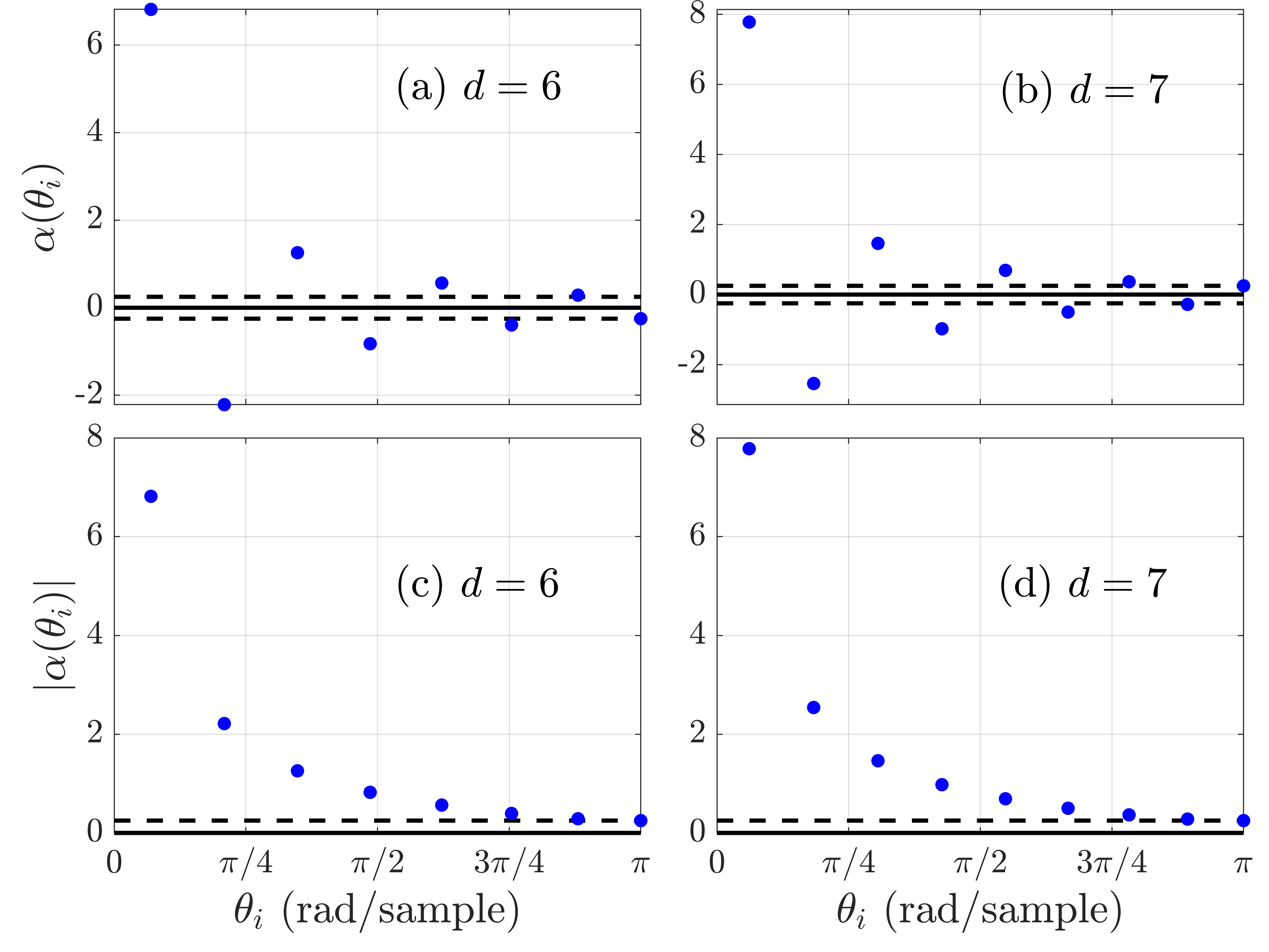
Figure 6: Example 2.4: For $p=\tfrac{1}{2}$, $d=6,$ and $d=7,$ (a) and (b) show $\alpha(\theta_{i})$ versus $\theta_{i}$, and (c) and (d) show $|\alpha(\theta_{i})|$ versus $\theta_{i}$. Note that the sign of $\alpha(\theta_{i})$ alternates. The dashed lines indicate $\pm\alpha_{\infty}=\pm\tfrac{1}{4}.$

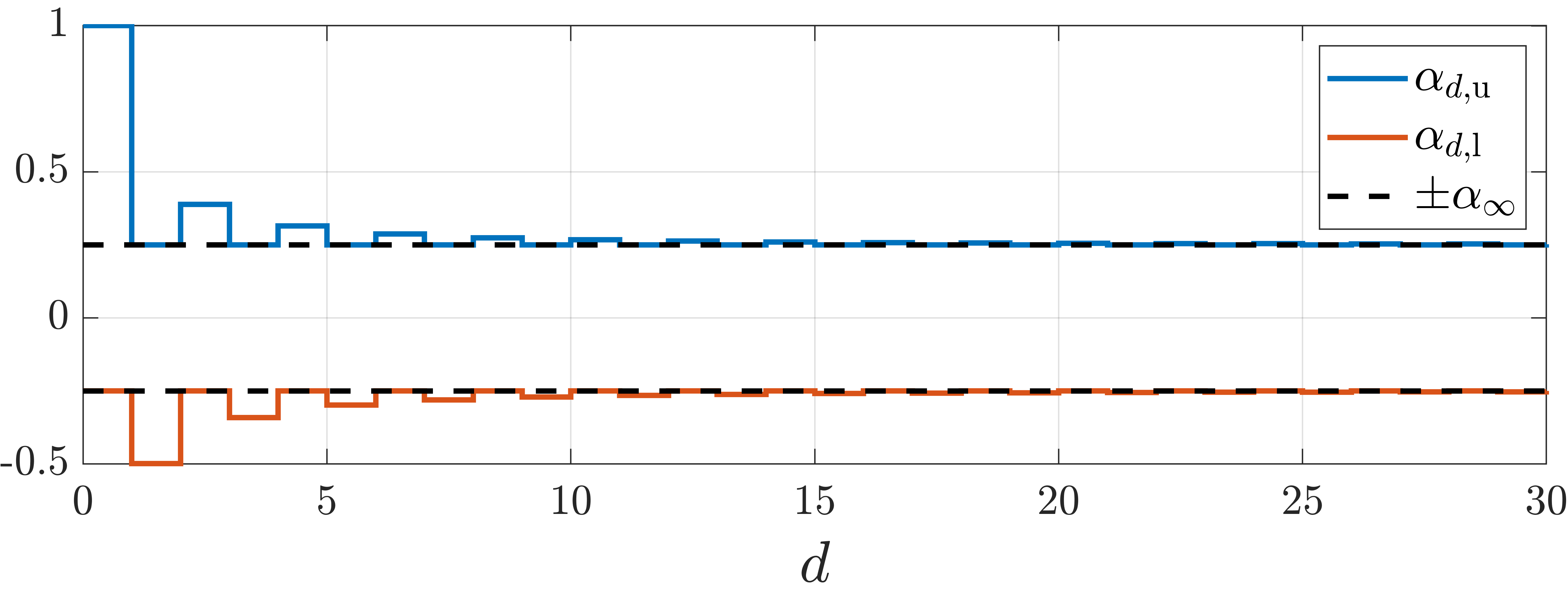
Figure 7: Example 2.4: For $p=\tfrac{1}{2}$, $\alpha_{d,{\rm l}}$ and $\alpha_{d,{\rm u}}$ versus $d$. As $d\to\infty,$ $\alpha_{d,{\rm l}}$ and $\alpha_{d,{\rm u}}$ converge to $-\alpha_{\infty}$ and $\alpha_{\infty}$, respectively, where $\alpha_{\infty}=\tfrac{1}{4}.$

Special case: For $p=0,$ (68) becomes

$$|\alpha(\theta)|=\frac{1}{\sqrt{2-2\cos\theta}},$$ (75)

and (69) becomes

$$\sin\,(d+1)\theta=\sin\,(d+2)\theta.$$ (76)

Note that, for all $i\in{\mathbb{Z}},$ $\sin(d+1)\theta=\sin[(2i+1)\pi-(d+1)\theta].$ Therefore, (76) holds if and only if $\theta=\frac{2k+1}{2d+3}\pi$. Hence, $\theta\in[0,\pi]$ satisfies (76) if and only if there exists $i\in\{0,\ldots,d+1\}$ such that $\theta_{k}\stackrel{{\scriptstyle\triangle}}{{=}}\left(\frac{2i+1}{2d+3}\right)\pi.$ For these $d+2$ values of $\theta,$ (2.4) implies that the corresponding values of $\alpha(\theta)$ are given by

$$\alpha(\theta_{i}) =\frac{\cos\theta_{i}}{\cos d\theta_{i}-\cos(d+1)\theta_{i}}$$

$$=\frac{\cos(d+1)\theta_{i}-\cos(d+2)\theta_{i}}{2-2\cos\theta_{i}}.$$ (77)

Next, it can be shown that, for all $i\in\{1,\ldots,d\},$ $\alpha(\theta_{i})\alpha(\theta_{i+1})<0$. Note that $\theta_{d+1}=\pi$ and $\alpha(\theta_{d+1})=(-1)^{d+1}\tfrac{1}{2}$. Hence, $|\alpha(\theta_{d+1})|=\tfrac{1}{2}.$ Furthermore, in the case where $d$ is even, $\alpha_{d,{\rm l}}=\alpha(\theta_{d+1})=-\tfrac{1}{2}<0$ and $\alpha_{d,{\rm u}}=\alpha(\theta_{d})>\tfrac{1}{2}>0,$ whereas, in the case where $d$ is odd, $\alpha_{d,{\rm l}}=\alpha(\theta_{d})<-\tfrac{1}{2}<0$ and $\alpha_{d,{\rm u}}=\alpha(\theta_{d+1})=\tfrac{1}{2}>0$. In addition, although $\lim_{d\to\infty}\alpha(\theta_{d})$ does not exist, it follows from (75) that $\lim_{d\to\infty}|\alpha(\theta_{d})|=\lim_{d\to\infty}\frac{1}{\sqrt{2-2\cos\left(\frac{2d+1}{2d+3}\right)\pi}}=\tfrac{1}{2}$, which confirms (26) and (74). For $d=10$ and $d=11$, Figure 8 shows $\alpha(\theta_{i})$ and $|\alpha(\theta_{i})|$ versus $\theta_{i}$. Note that, for both values of $d,$ the minimum value of $|\alpha(\theta_{i})|$ is $\tfrac{1}{2}$, which occurs at $\theta=\pi$. Finally, Figure 9 shows $\alpha_{d,{\rm l}}$ and $\alpha_{d,{\rm u}}$ versus $d,$ which indicates that $\lim_{d\to\infty}\alpha_{d,{\rm l}}=-\tfrac{1}{2}$ and $\lim_{d\to\infty}\alpha_{d,{\rm u}}=\tfrac{1}{2}.$ $\diamond$

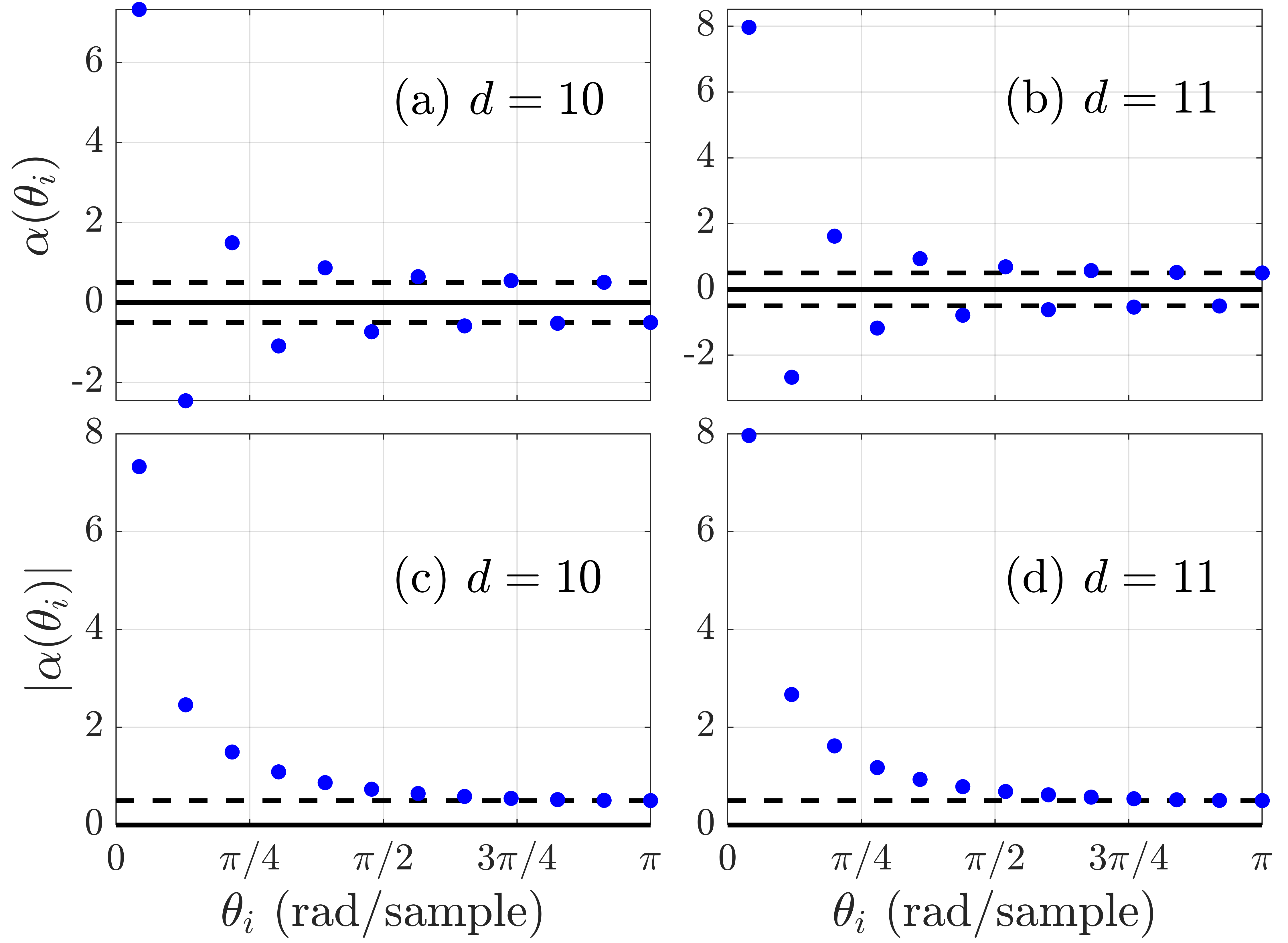
Figure 8: Example 2.4: For $p=0,$ $d=10,$ and $d=11,$ (a) and (b) show $\alpha(\theta_{i})$ versus $\theta_{i}$, and (c) and (d) show $|\alpha(\theta_{i})|$ versus $\theta_{i}$. The dashed lines indicate $\pm\alpha_{\infty}=\pm\tfrac{1}{2}.$

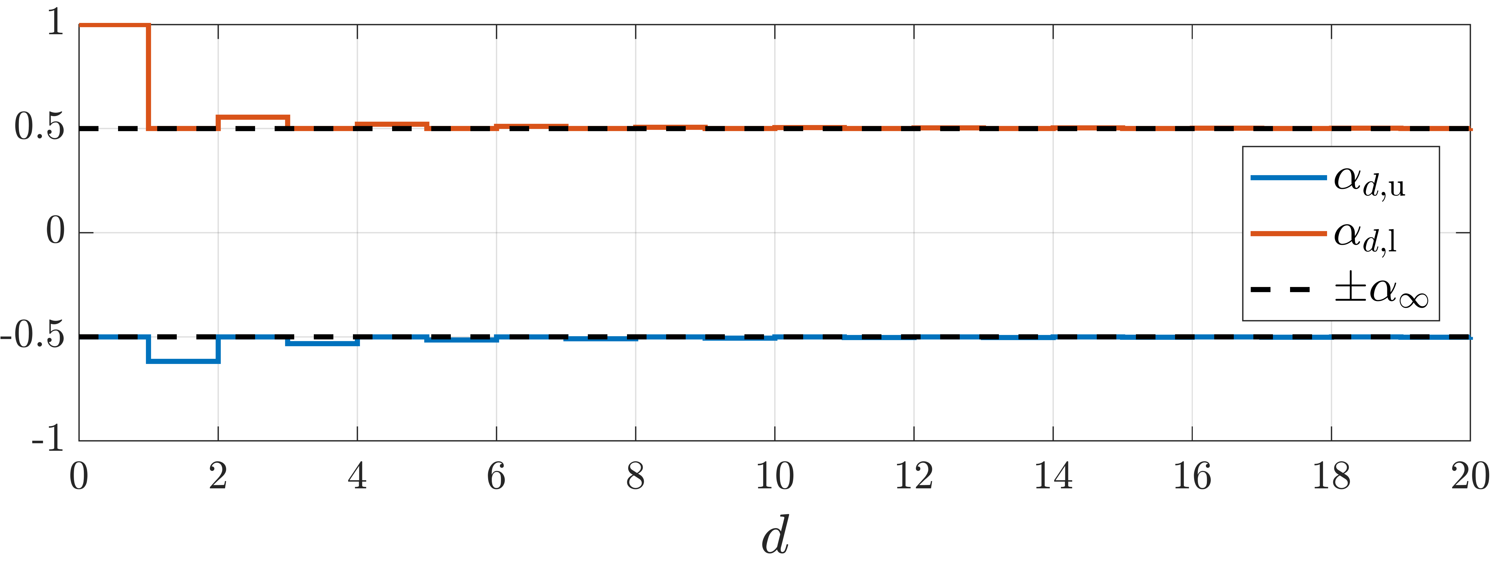
Figure 9: Example 2.4: For $p=0$, $\alpha_{d,{\rm l}}$ and $\alpha_{d,{\rm u}}$ versus $d$. As $d\to\infty,$ $\alpha_{d,{\rm l}}$ and $\alpha_{d,{\rm u}}$ converge to $-\alpha_{\infty}$ and $\alpha_{\infty}$, respectively, where $\alpha_{\infty}=\tfrac{1}{2}.$

Example 2.5

Let

$$G(z)=\frac{N(z)}{D(z)}=\frac{z+0.2\pm\jmath 0.79}{z(z-0.25\pm\jmath 0.95)}.$$

Figure 10 shows that, for all $d\geq 1,$ there exists $\alpha_{d,{\rm l}}<0$ such that $p_{d,\alpha}$ if and only if $\alpha\in(\alpha_{d,{\rm l}},0]$ as stated in iv) from Theorem 2.2. Furthermore, define

$$\alpha_{\rm uc}(\theta)\stackrel{{\scriptstyle\triangle}}{{=}}\left|\frac{D(e^{\jmath\theta})}{(e^{\jmath\theta}-1)N(e^{\jmath\theta})}\right|=\left|\frac{(e^{\jmath\theta}-0.25\pm\jmath 0.95)}{(e^{\jmath\theta}-1)(e^{\jmath\theta}+0.2\pm\jmath 0.79)}\right|,$$

such that $\alpha_{\infty}=\min_{\theta\in(0,\pi]}\alpha_{\rm uc}(\theta).$ Figure 11 shows that $\alpha_{\rm uc}$ has a minimum at $\theta\approx 0.4180\pi,$ which implies that $\alpha_{\infty}\approx\alpha_{\rm uc}(0.4180\pi)=0.0313.$ Finally, Figure 12 shows $\alpha_{d,{\rm l}}$ and $\alpha_{d,{\rm u}}$ versus $d\geq 1,$ which shows that $\lim_{d\to\infty}\alpha_{d,{\rm l}}=-\alpha_{\infty}$ and $\lim_{d\to\infty}\alpha_{d,{\rm u}}=\alpha_{\infty},$ as stated in v) from Theorem 2.2. $\diamond$

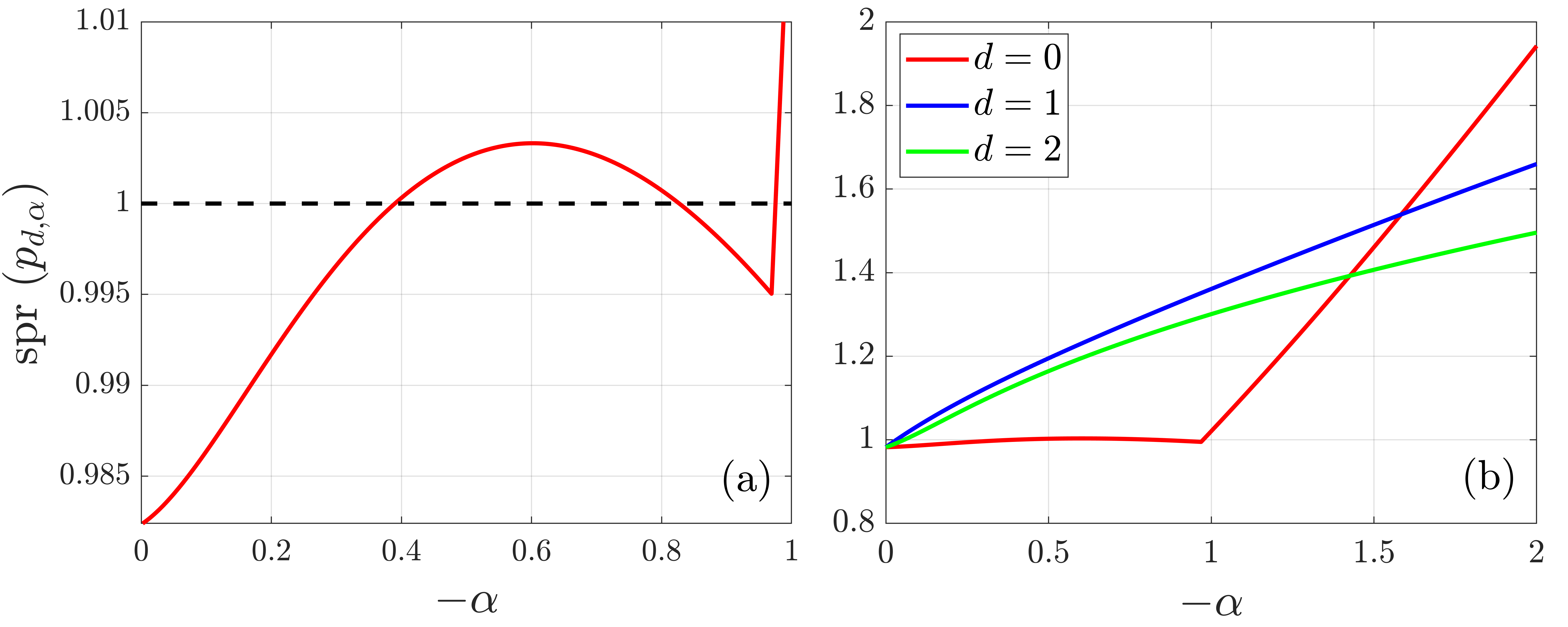
Figure 10: Example 2.5: $\operatorname{spr}(p_{d,\alpha})$ versus $-\alpha,$ for $\alpha\leq 0.$ (a) shows that, for $d=0,$ $\alpha_{0,{\rm l}}$ as defined in iv) from Theorem 2.2 doesn’t exist. (b) shows that, for $d\geq 1,$ $\alpha_{0,{\rm l}}$ as defined in iv) from Theorem 2.2 exists.

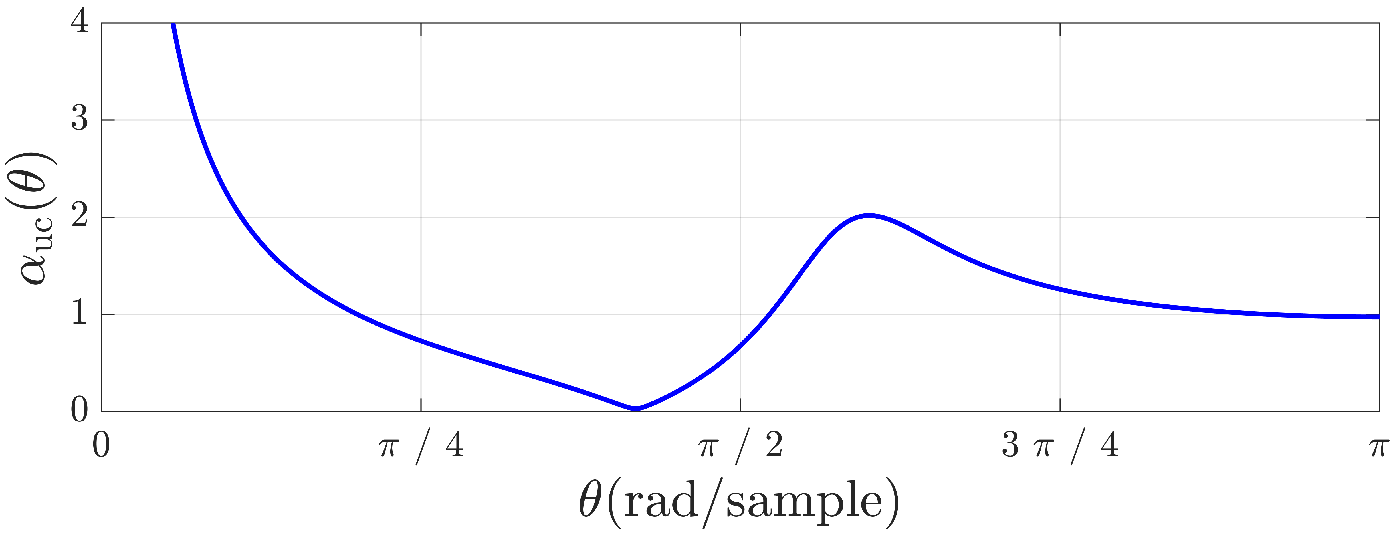
Figure 11: Example 2.5: $\alpha_{\rm uc}(\theta)$ versus $\theta$ for $\theta\in(0,\pi].$ Note that $\lim_{\theta\downarrow 0}\alpha_{\rm uc}(\theta)=\infty$ and that $\min_{\theta\in(0,\pi]}\alpha_{\rm uc}(\theta)=\alpha_{\rm uc}(\theta_{\infty})\approx 0.0313,$ where $\theta_{\infty}\approx 0.4180\pi.$

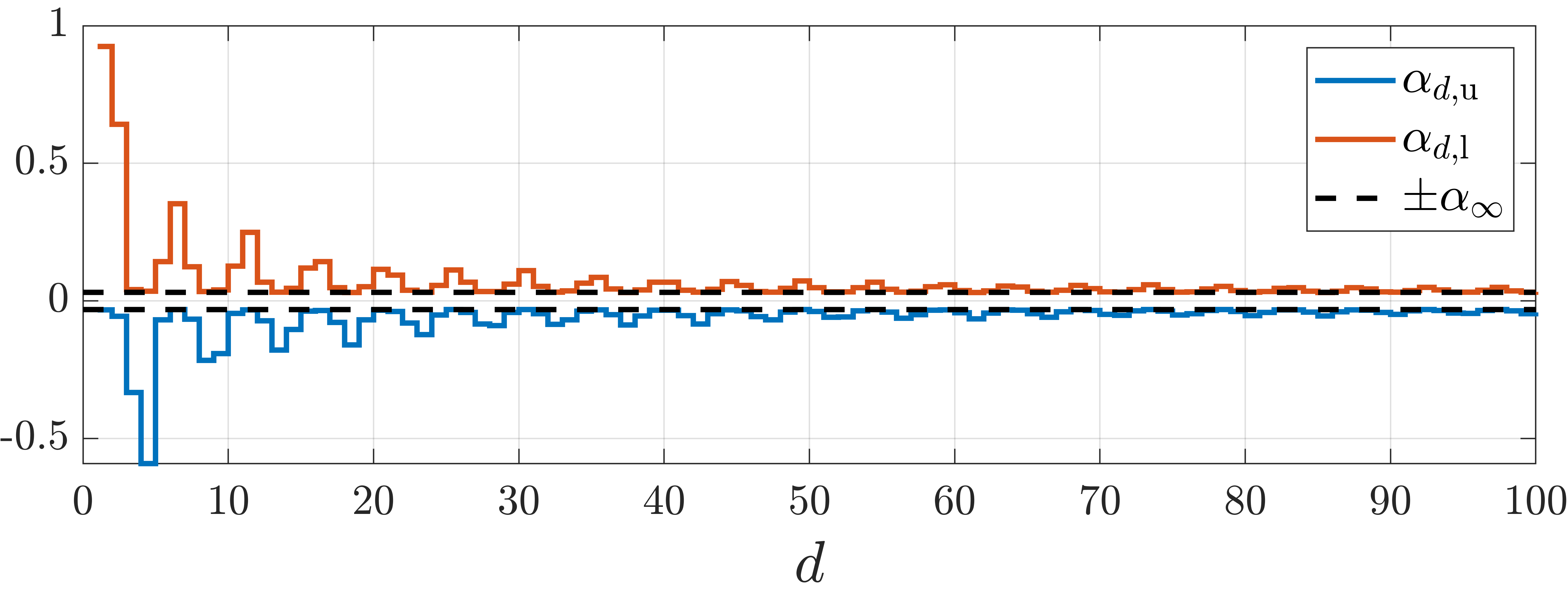
Figure 12: Example 2.5: $\alpha_{d,{\rm l}}$ and $\alpha_{d,{\rm u}}$ versus $d\geq 1.$ As $d\to\infty,$ $\alpha_{d,{\rm l}}$ and $\alpha_{d,{\rm u}}$ converge to $-\alpha_{\infty}$ and $\alpha_{\infty}$, respectively, where $\alpha_{\infty}\approx 0.0313.$

3 Time-Delayed Lur’e Model

Inserting the saturation nonlinearity following the washout filter $W$ in Figure 5 yields the TDL model shown in Figure 13, which has the closed-loop dynamics

$$\left[\begin{array}[]{c}x_{k+1}\\ x_{{\rm d},k+1}\\ x_{{\rm f},k+1}\end{array}\right]=\left[\begin{array}[]{ccc}A&0&0\\ e_{d,d}C&N_{d}&0\\ 0&e_{1,d}^{\rm T}&0\end{array}\right]\left[\begin{array}[]{c}x_{k}\\ x_{{\rm d},k}\\ x_{{\rm f},k}\end{array}\right]+\left[\begin{array}[]{c}\alpha B\\ 0\\ 0\end{array}\right]v_{{\rm f},k},$$ (90)

with $y_{k},$ $y_{{\rm d},k},$ and $y_{{\rm f},k}$ given by (15), (16), and (17), respectively, where $v_{{\rm f},k}={\rm sat}_{\delta}(y_{{\rm f},k})$ is the output of the saturation function ${\rm sat}_{\delta}\colon{\mathbb{R}}\to{\mathbb{R}}$, where $\delta>0,$ defined by

$${\rm sat}_{\delta}(u)=\begin{cases}u,&|u|\leq\delta,\\ {\rm sign}(u),&|u|>\delta.\end{cases}$$ (91)

Figure 13: Discrete-time time-delayed Lur’e model.

To analyze the self-oscillating behavior of the time-delayed Lur’e model, we replace the saturation nonlinearity by its describing function. Describing functions are used to characterize self-excited oscillations in [2, Section 5.4] and [15, pp. 293–294]. The describing function $\Psi_{\delta}(\varepsilon)$ for $\rm sat_{\delta}$ for a sinusoidal input with amplitude $\varepsilon>0$ is given by

$$\Psi_{\delta}(\varepsilon) =\begin{cases}\frac{2}{\pi}\left[\sin^{-1}\left(\frac{\delta}{\varepsilon}\right)+\left(\frac{\delta}{\varepsilon}\right)\sqrt{1-\left(\frac{\delta}{\varepsilon}\right)^{2}}\right],&\text{if }\varepsilon>\delta\\ 1,&\text{otherwise}.\end{cases}$$ (92)

Note that, for $\varepsilon>\delta$, the function $\Psi_{\delta}$ confined to $(\delta,\infty)$ with codomain $(0,1)$ is decreasing, one-to-one, and onto. Let $p_{d,\alpha,\varepsilon}$ be the characteristic polynomial of the linearized time-delay Lur’e model, such that

$$p_{d,\alpha,\varepsilon}(z)\stackrel{{\scriptstyle\triangle}}{{=}}z^{d+1}D(z)-\alpha\Psi_{\delta}(\varepsilon)(z-1)N(z).$$ (93)

For all $\varepsilon_{\rm l}>0,$ $\varepsilon_{\rm u}>0,$ $\theta_{\rm l}\in{\mathbb{R}},$ and $\theta_{\rm u}\in{\mathbb{R}}$ such that $\varepsilon_{\rm l}<\varepsilon_{\rm u}$ and $\theta_{\rm l}<\theta_{\rm u},$ define the rectangle

$$\Gamma_{\theta_{\rm l},\theta_{\rm u},\varepsilon_{\rm l},\varepsilon_{\rm u}}\stackrel{{\scriptstyle\triangle}}{{=}}\{(\theta,\varepsilon)\colon\theta_{\rm l}<\theta<\theta_{\rm u}\mbox{ and }\varepsilon_{\rm l}<\varepsilon<\varepsilon_{\rm u}\}$$

Lemma 3.1

Let $\alpha\in\mathbb{R},$ and let $\theta_{0}\in\Theta$ be such that $\operatorname{sign}\alpha_{0}=\operatorname{sign}\alpha$ and $|\alpha_{0}|<|\alpha|$, where $\alpha_{0}\stackrel{{\scriptstyle\triangle}}{{=}}\alpha(\theta_{0}),$ and let $d>\bar{d}$. Then, the following statements hold:

1. There exist $\varepsilon_{0}>0$, $\theta_{\rm l}>0,$ $\theta_{\rm u}>0,$ $\varepsilon_{\rm l}>0,$ and $\varepsilon_{\rm u}>0$ such that $\varepsilon_{\rm l}<\varepsilon_{\rm u},$ $\theta_{\rm l}<\theta_{\rm u},$ $(\theta_{0},\varepsilon_{0})\in\Gamma_{\theta_{\rm l},\theta_{\rm u},\varepsilon_{\rm l},\varepsilon_{\rm u}},$ and, in the rectangle $\Gamma_{\theta_{\rm l},\theta_{\rm u},\varepsilon_{\rm l},\varepsilon_{\rm u}}$, $(\theta,\varepsilon)=(\theta_{0},\varepsilon_{0})$ is the unique solution of $p_{d,\alpha,\varepsilon}(e^{\jmath\theta})=0$.

2. $$\left.\frac{{\rm d}}{{\rm d}\varepsilon}\Psi_{\delta}(\varepsilon)\right\rvert_{\varepsilon=\varepsilon_{0}}\neq 0.$$ (94)

3. $$\left.\frac{{\rm d}}{{\rm d}\theta}{\rm Im}[L_{d}(e^{\jmath\theta})]\right\rvert_{\theta=\theta_{0}}\neq 0.$$ (95)

Proof. To prove $i),$ note that, for $\operatorname{sign}\alpha_{0}=\operatorname{sign}\alpha$ and $|\alpha_{0}|>|\alpha|$, there exists $\varepsilon_{0}>\delta$ such that $\alpha_{0}=\Psi_{\delta}(\varepsilon_{0})\alpha$. Therefore, $p_{d,\alpha_{0}}(e^{\jmath\theta_{0}})=p_{d,\alpha,\varepsilon_{0}}(e^{\jmath\theta_{0}})=0.$ Furthermore, there exists a rectangle $\Gamma_{\theta_{\rm l},\theta_{\rm u},\varepsilon_{\rm l},\varepsilon_{\rm u}},$ where $\theta_{\rm l}>0,$ $\theta_{\rm u}>0,$ $\varepsilon_{\rm l}>0,$ $\varepsilon_{\rm u}>0,$ $\varepsilon_{\rm l}<\varepsilon_{\rm u}$ and $\theta_{\rm l}<\theta_{\rm u},$ such that $(\theta_{0},\varepsilon_{0})\in\Gamma_{\theta_{\rm l},\theta_{\rm u},\varepsilon_{\rm l},\varepsilon_{\rm u}}$ and $\Theta\cap(\theta_{\rm l},\theta_{\rm u})=\theta_{0}.$ Hence, in the rectangle $\Gamma_{\theta_{\rm l},\theta_{\rm u},\varepsilon_{\rm l},\varepsilon_{\rm u}}$, $(\theta,\varepsilon)=(\theta_{0},\varepsilon_{0})$ is the unique solution of $p_{d,\alpha,\varepsilon}(e^{\jmath\theta})=0$.

To prove $ii),$ note that

$$\left.\frac{{\rm d}}{{\rm d}\varepsilon}\Psi_{\delta}(\varepsilon)\right\rvert_{\varepsilon=\varepsilon_{0}}=-\frac{4\delta\sqrt{\varepsilon_{0}^{2}-\delta^{2}}}{\pi\varepsilon_{0}^{3}}<0.$$ (96)

To prove $iii)$, writing $G(e^{\jmath\theta})=a_{n}-\jmath b_{n},$ where $a_{n}=\frac{a}{a^{2}+b^{2}}$ and $b_{n}=\frac{b}{a^{2}+b^{2}}.$ Then,

$$L_{d} (e^{\jmath\theta})=G(e^{\jmath\theta})G_{d}(e^{\jmath\theta})W(e^{\jmath\theta})$$

$$=(a_{n}-\jmath b_{n})(e^{-\jmath d\theta}-e^{-\jmath(d+1)\theta})$$

$$=(a_{n}(\cos d\theta-\cos\,(d+1)\theta)-b_{n}(\sin d\theta-\sin\,(d+1)\theta))$$

$$+\jmath(-a_{n}(\sin d\theta-\sin\,(d+1)\theta)-b_{n}(\cos d\theta-\cos\,(d+1)\theta))$$

$$=\frac{f}{a^{2}+b^{2}}-\jmath\frac{g}{a^{2}+b^{2}}.$$ (97)

Since $\theta_{0}\in\Theta$ and $\alpha(\theta_{0})\neq 0$, it follows from (60) and (3) with $\theta=\theta_{0}$ that $g=0$ and thus

$${\rm Re}[L_{d}(e^{\jmath\theta_{0}})]\neq 0,\quad{\rm Im}[L_{d}(e^{\jmath\theta_{0}})]=0.$$ (98)

Furthermore, differentiating $\angle L_{d}(e^{\jmath\theta})$ with respect to $\theta$ yields

$$\frac{{\rm d}}{{\rm d}\theta}\angle L_{d}(e^{\jmath\theta})=\frac{{\rm d}}{{\rm d}\theta}{\rm atan}\left(\frac{{\rm Im}[L_{d}(e^{\jmath\theta})]}{{\rm Re}[L_{d}(e^{\jmath\theta})]}\right)$$

$$=\frac{{\rm Re}[L_{d}(e^{\jmath\theta})]\frac{{\rm d}}{{\rm d}\theta}{\rm Im}[L_{d}(e^{\jmath\theta})]-{\rm Im}[L_{d}(e^{\jmath\theta})]\frac{{\rm d}}{{\rm d}\theta}{\rm Re}[L_{d}(e^{\jmath\theta})]}{|L_{d}(e^{\jmath\theta})|}.$$ (99)

It follows from (98) and (3) that

$$\left.\frac{{\rm d}}{{\rm d}\theta}\angle L_{d}(e^{\jmath\theta})\right\rvert_{\theta=\theta_{0}}=\frac{{\rm Re}[L_{d}(e^{\jmath\theta_{0}})]\left.\frac{{\rm d}}{{\rm d}\theta}{\rm Im}[L_{d}(e^{\jmath\theta})]\right\rvert_{\theta=\theta_{0}}}{|L_{d}(e^{\jmath\theta_{0}})|}.$$ (100)

It follows from (24) that, for all $d>\bar{d},$ $\left.\frac{{\rm d}}{{\rm d}\theta}\angle L_{d}(e^{\jmath\theta})\right\rvert_{\theta=\theta_{0}}<0.$ Hence, it follows from (100) that $\left.\frac{{\rm d}}{{\rm d}\theta}{\rm Im}[L_{d}(e^{\jmath\theta})]\right\rvert_{\theta=\theta_{0}}\neq 0.$ $\square$

Theorem 3.2

Consider the discrete-time time-delayed Lur’e model in Figure 13, assume that $x_{0}\neq 0,$ and let $\alpha\in(-\infty,\alpha_{d,{\rm l}})\cup(\alpha_{d,{\rm u}},\infty).$ Then, there exists a nonconstant periodic function $\tau\colon{\mathbb{N}}\to{\mathbb{R}}$ such that $\lim_{k\to\infty}|y_{k}-\tau_{k}|=0.$

Proof. Lemma 3.1 implies that the assumptions of Theorem 7.4 in [15, pp. 293, 294] are satisfied. It thus follows that the response is asymptotically periodic. $\square$

It can be seen that Theorem 3.2 holds in the case where the saturation function is replaced by an odd sigmoidal nonlinearity such as atan or tanh.

Example 3.3

Let $G(z)\mspace{-4.0mu}=\mspace{-5.0mu}1/z.$ Figure 14 shows the transient response and asymptotic oscillatory response for $\alpha=1.1$, $d=0$, and $\delta=1$ along with plot of $v_{{\rm f},k}$ and $y_{{\rm f},k}$. Figure 14(a) shows that, for $k>80$, $y_{k}$ is a nonconstant periodic function. Furthermore, Figure 14(b) shows how the saturation nonlinearity acts upon $y_{{\rm f},k},$ which results in the saturated signal $v_{{\rm f},k}\in[-\delta,\delta].$ Note that $v_{{\rm f},k}$ and $y_{{\rm f},k}$ are also nonconstant periodic functions for $k>80.$

Figure 15 shows $\alpha(\theta_{i})$ versus $\theta_{i}$ for $d=0$ and $d=1$. For $\alpha=0.6$, only in the case $d=1$ has $\alpha(\theta_{i})$ such that $\rm sign(\alpha(\theta_{i}))=\rm sign(\alpha)$ and $|\alpha(\theta_{i})|<|\alpha|$. For $\alpha=1.1$, both models meet the conditions for $\alpha$.

Figure 16 shows the response of $y_{k}$ for $\delta=1$ and all possible pairs of $d=0,1$ and $\alpha=0.6,1.1$. For $\alpha=0.6$, only the model with $d=1$ yields a limit cycle. For $\alpha=1.1$, both models yield oscillations. This follows from the conditions for $\alpha$ stated in the previous paragraph and in Lemma 3.1.

Finally, Figure 17 shows the magnitude of the frequency response for models with $\alpha=1.1,$ $\delta=1,$ and $d=0,1.$ Note that the frequencies corresponding to the magnitude peaks are similar to the values of $\theta_{i}$ shown in Figure 15 such that $\rm sign(\alpha(\theta_{i}))=\rm sign(\alpha)$ and $|\alpha(\theta_{i})|<|\alpha|$. $\diamond$

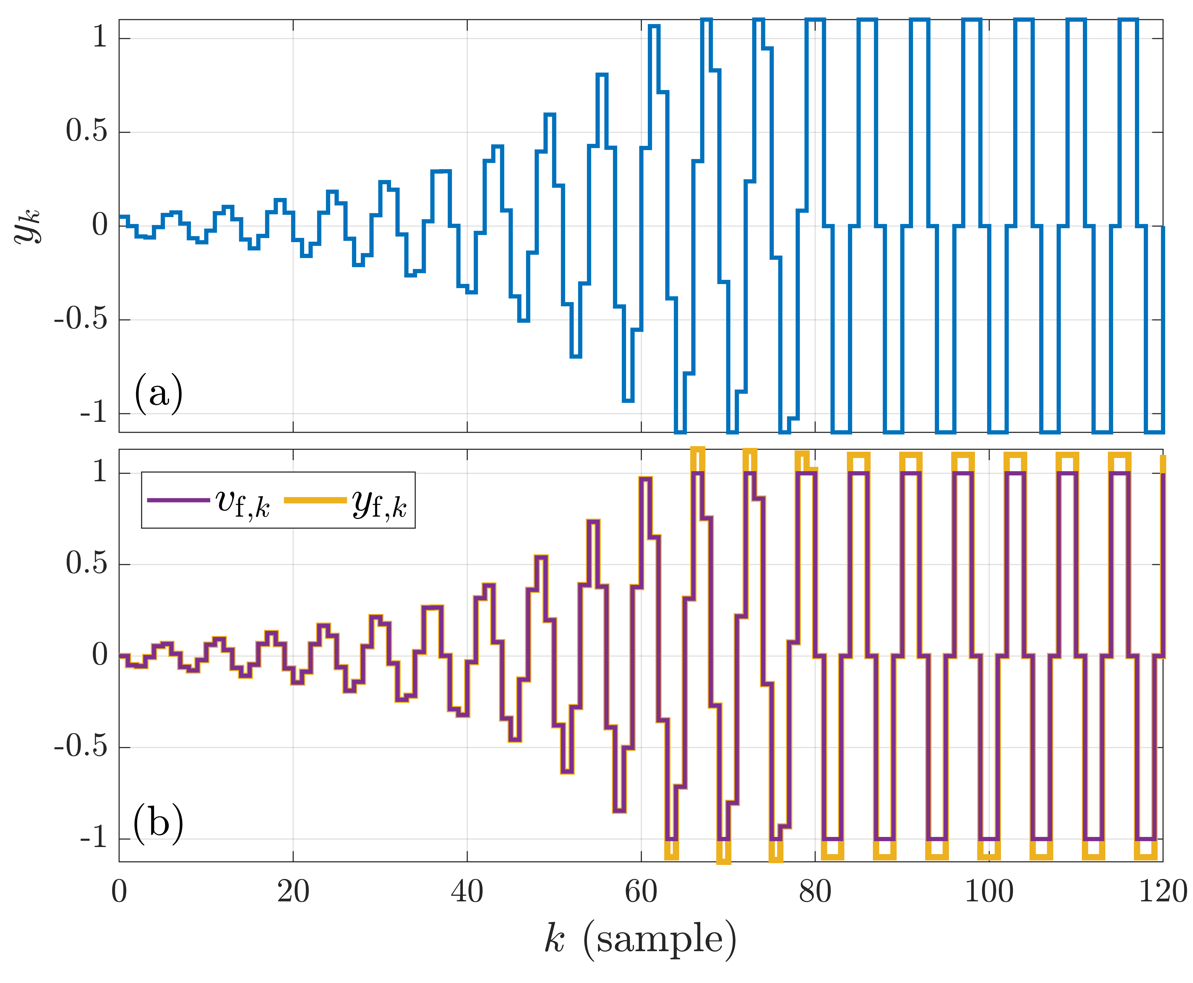
Figure 14: Example 3.3: For $d=0$, $\delta=1,$ and $\alpha=1.1,$ (a) shows $y_{k},$ and (b) shows $v_{{\rm f},k}$ and $y_{{\rm f},k}$. The saturation nonlinearity, with $\delta=1,$ saturates the values of $y_{{\rm f},k},$ resulting in $v_{{\rm f},k}\in[-\delta,\delta].$

Figure 15: Example 3.3: For $d=0$ and $d=1$, these plots show the values $\alpha(\theta_{i})$ of $\alpha$ for which the closed-loop dynamics have a pole on the unit circle at the angle $\theta_{i}$ for $i=1,\ldots,d+2.$ For the case $d=0,$ where $\theta_{1}=1.0472$ and $\theta_{2}=\pi$, the time-delayed Lur’e model has self-excited oscillations if and only if either $\alpha>1$ or $\alpha<-\tfrac{1}{2},$ while, for the case $d=1,$ where $\theta_{1}=0.6283$, $\theta_{2}=1.8850$ and $\theta_{3}=\pi$, the TDL model has self-excited oscillations if and only if either $\alpha>\tfrac{1}{2}$ or $\alpha<-0.618.$ For all values of $\alpha$ corresponding to the shaded regions, the response of the TDL model oscillates.

Figure 16: Example 3.3: Response $y_{k}$ of the TDL model for $d=0,1$ and $\alpha=0.6,1.1$ with $\delta=1$.

Figure 17: Example 3.3: Frequency response of $y_{k}$ for $d=0,1$ with $\alpha=1.1$ and $\delta=1$. Note that, for $d=0,$ the peak is located at $\theta_{1}$, whereas, for $d=1,$ the peak is located at $\theta_{3}.$

4 Time-Delayed Lur’e Model with Bias Generation

We now modify the discrete-time time-delay Lur’e model by including the bias-generation mechanism shown in Figure 1. The corresponding closed-loop dynamics are thus given by

$$\left[\begin{array}[]{c}x_{k+1}\\ x_{{\rm d},k+1}\\ x_{{\rm f},k+1}\end{array}\right]=\left[\begin{array}[]{ccc}A&0&0\\ e_{d,d}C&N_{d}&0\\ 0&e_{1,d}^{\rm T}&0\end{array}\right]\left[\begin{array}[]{c}x_{k}\\ x_{{\rm d},k}\\ x_{{\rm f},k}\end{array}\right]+\left[\begin{array}[]{c}B\\ 0\\ 0\end{array}\right]v_{{\rm b},k},$$ (113)

with $y_{k},$ $y_{{\rm d},k},$ and $y_{{\rm f},k}$ given by (15), (16), and (17), respectively, where $\beta$ is a constant,

$$v_{{\rm b},k}=(\beta+v_{{\rm f},k})v_{k},$$ (114)

and $v_{{\rm f},k}={\rm sat}_{\delta}(y_{{\rm f},k}).$ Note that the constant $\alpha$ is now omitted. Instead, the constant input $v$ is injected multiplicatively inside the loop, thus playing the role of $\alpha$. This feature allows the offset of the oscillation to depend on the external input. The resulting bias $\bar{y}$ of the periodic response is thus given by

$$\bar{y}=v\beta G(1).$$ (115)

Figure 18: Discrete-time time-delayed Lur’e model with constant input $v$ and bias generation.

Example 4.1

Let $G(z)\mspace{-2.0mu}=\mspace{-2.0mu}1/z,$ $d\mspace{-2.0mu}=\mspace{-2.0mu}0,$ $\beta=2.5,$ $v\mspace{-2.0mu}=\mspace{-2.0mu}1.1,$ and $\delta\mspace{-2.0mu}=\mspace{-2.0mu}1.$ Figure 19(a) shows that the output $y_{k}$ is oscillatory with offset $\bar{y}=v\beta G(1)=2.75.$ Figure 19(b) shows $v_{{\rm f},k}$ and $y_{{\rm f},k}.$ Note that, as in Example 3.3, despite the offset $\bar{y}$ of $y_{k}$, the signals $y_{{\rm f},k}$ and $v_{{\rm f},k}$ oscillate without an offset. Finally, Figure 19(c) shows the magnitude of the frequency response for $y_{k}-\bar{y}$. Note that the peak is located near the same frequency as in Example 3.3, and thus the oscillation frequency remains the same with the addition of the bias-generation mechanism. $\diamond$

Figure 19: Example 4.1: For $v=1.1,$ $\beta=2.5,$ $d=0,$ and $\delta=1,$ (a) shows $y_{k}$ and the offset $\bar{y}$, (b) shows $v_{{\rm f},k}$ and $y_{{\rm f},k},$ and (c) shows the frequency response of $y_{k}-\bar{y}.$

Example 4.2

Let

$$G(z)=\frac{z-0.75e^{\pm\jmath 5\pi/6}}{(z-0.9e^{\pm\jmath\pi/6})(z-0.9e^{\pm\jmath 5\pi/12})},$$

$d=4,$ $\beta=15$ $v=1,$ and $\delta=1.$ Figure 20(a) shows that the output $y_{k}$ is oscillatory with offset $\bar{y}=v\beta G(1)=5.751.$ Figure 20(b) shows that $v_{{\rm f},k}$ and $y_{{\rm f},k}$ have an oscillatory response without an offset, as in previous cases. Finally, Figure 20(c) shows the magnitude of the frequency response for $y_{k}-\bar{y}$. $\diamond$

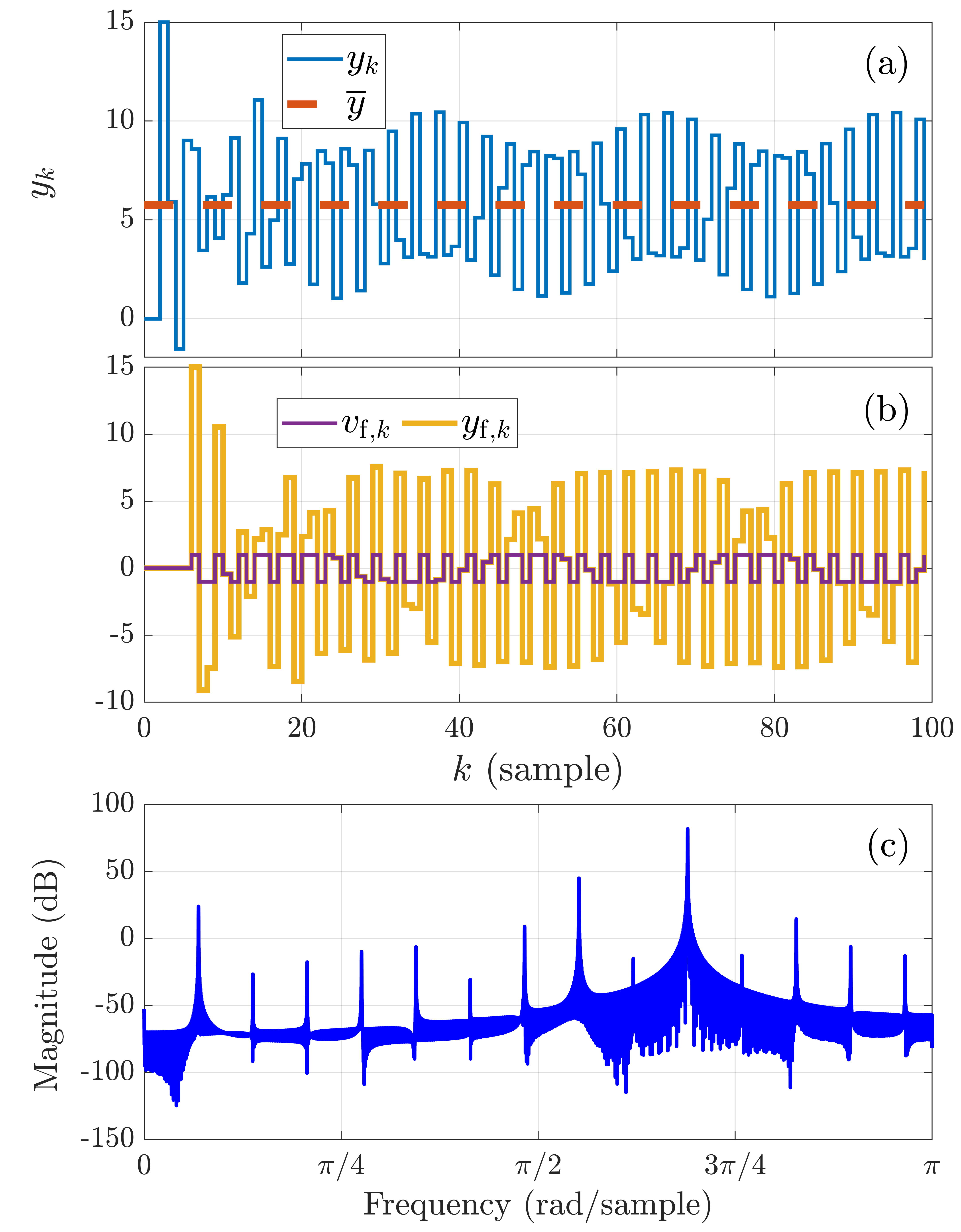
Figure 20: Example 4.2: For $v=1,$ $\beta=15,$ $d=4,$ and $\delta=1,$ (a) shows $y_{k}$ and the offset $\bar{y}$, (b) shows $v_{{\rm f},k}$ and $y_{{\rm f},k},$ and (c) shows the frequency response of $y_{k}-\bar{y}.$

5 Conclusions and Future Extensions

This paper presented and analyzed a discrete-time Lur’e model that exhibits self-excited oscillations. This model involves an asymptotically stable linear system, a time delay, a washout filter, and a saturation nonlinearity. It was shown that, for sufficiently large loop gains, the response converges to a periodic signal, and thus the system has self-excited oscillations. A bias-generation mechanism provides an input-dependent oscillation offset. The amplitude and spectral content of the oscillation were analyzed in terms of the components of the model.

An immediate extension of this work is to consider the case where $G$ has zeros on the unit circle. The main results of this paper appear to be valid for this case, although the proofs are more intricate. Extension to sigmoidal nonlinearities such as atan and tanh as well as relay nonlinearities is of interest. In addition, continuous-time, time-delay Lur’e models described by iv) in Section I are of interest. Finally, future work will use this discrete-time self-excited model for system identification and adaptive stabilization.

6 Acknowledgments

This research was supported by NSF grant CMMI 1634709, “A Diagnostic Modeling Methodology for Dual Retrospective Cost Adaptive Control of Complex Systems.”

Author Biographies

Juan Paredes received the B.Sc. degree in mechatronics engineering from the Pontifical Catholic University of Peru and a M.Sc. degree in aerospace engineering from the University of Michigan in Ann Arbor, MI. He is currently a PhD candidate in the Aerospace Engineering Department at the University of Michigan. His interests are in autonomous flight control and control of combustion.

Syed Aseem Ul Islam received the B.Sc. degree in aerospace engineering from the Institute of Space Technology, Islamabad and is currently pursuing the Ph.D. degree in flight dynamics and control from the University of Michigan in Ann Arbor. His interests are in data-driven adaptive control for aerospace applications.

Omran Kouba received the Sc.B. degree in Pure Mathematics from the University of Paris XI and the Ph.D. degree in Functional Analysis from Pierre and Marie Curie University in Paris, France. Currently he is a professor in the Department of Mathematics in the Higher Institute of Applied Sciences and Technology, Damascus (Syria). His interests are in real and complex analysis, inequalities, and problem solving.

Dennis S. Bernstein received the Sc.B. degree from Brown University and the Ph.D. degree from the University of Michigan in Ann Arbor, Michigan, where he is currently professor in the Aerospace Engineering Department. His interests are in identification, estimation, and control for aerospace applications. He is the author of Scalar, Vector, and Matrix Mathematics, published by Princeton University Press.

References

- [1] A. Jenkins, “Self-oscillation,” Physics Reports, vol. 525, no. 2, pp. 167–222, 2013.
- [2] W. Ding, Self-Excited Vibration: Theory, Paradigms, and Research Methods. Springer, 2010.
- [3] B. Chance, E. K. Pye, A. K. Ghosh, and B. Hess, Eds., Biological and Biochemical Oscillators. Academic Press, 1973.
- [4] P. Gray and S. K. Scott, Chemical Oscillations and Instabilities: Non-linear Chemical Kinetics. Oxford, 1990.
- [5] A. Goldbeter and M. J. Berridge, Biochemical Oscillations and Cellular Rhythms: The Molecular Bases of Periodic and Chaotic Behaviour. Cambridge, 1996.
- [6] A. P. Dowling, “Nonlinear Self-Excited Oscillations of a Ducted Flame,” J. Fluid Mech., vol. 346, pp. 271–291, 1997.
- [7] E. Awad and F. E. C. Culick, “On the existence and stability of limit cycles for longitudinal acoustic modes in a combustion chamber,” Combustion Science and Technology, vol. 46, pp. 195–222, 1986.
- [8] Y. Chen and J. F. Driscoll, “A multi-chamber model of combustion instabilities and its assessment using kilohertz laser diagnostics in a gas turbine model combustor,” Combustion and Flame, vol. 174, pp. 120–137, 2016.
- [9] M. Münnich, M. A. Cane, and S. E. Zebiak, “A study of self-excited oscillations of the tropical ocean–atmosphere system. part ii: Nonlinear cases,” Journal of the Atmospheric Sciences, vol. 48, no. 10, pp. 1238–1248, 1991.
- [10] R. D. Blevins, Flow-Induced Vibration. Van Nostrand Reinhold, 1990.
- [11] P. P. Friedmann, “Renaissance of aeroelasticity and its future,” J. Aircraft, vol. 36, pp. 105–121, 1999.
- [12] B. D. Coller and P. A. Chamara, “Structural non-linearities and the nature of the classic flutter instability,” J. Sound Vibr., vol. 277, pp. 711–739, 2004.
- [13] E. Jonsson, C. Riso, C. A. Lupp, C. E. S. Cesnik, J. R. R. A. Martins, and B. I. Epureanu, “Flutter and post-flutter constraints in aircraft design optimization,” Progress in Aerospace Sciences, vol. 109, p. 100537, August 2019.
- [14] R. Scott, In the Wake of Tacoma: Suspension Bridges and the Quest for Aerodynamic Stability. ASCE Press, 2001.
- [15] H. K. Khalil, Nonlinear Systems, 3rd ed. Prentice Hall, 2002.
- [16] X. Jian and C. Yu-shu, “Effects of time delayed velocity feedbacks on self-sustained oscillator with excitation,” Applied Mathematics and Mechanics, vol. 25, no. 5, pp. 499–512, May 2004.
- [17] D. H. Zanette, “Self-sustained oscillations with delayed velocity feedback,” Papers in Physics, vol. 9, pp. 090 003–1–090 003–7, March 2017.
- [18] S. Risau-Gusman, “Effects of time-delayed feedback on the properties of self-sustained oscillators,” Phys. Rev. E, vol. 94, p. 042212, October 2016.
- [19] S. Chatterjee, “Self-excited oscillation under nonlinear feedback with time-delay,” Journal of Sound and Vibration, vol. 330, no. 9, pp. 1860–1876, 2011.
- [20] G. Stan and R. Sepulchre, “Analysis of interconnected oscillators by dissipativity theory,” IEEE Transactions on Automatic Control, vol. 52, no. 2, pp. 256–270, 2007.
- [21] E. A. Tomberg and V. A. Yakubovich, “Conditions for auto-oscillations in nonlinear systems,” Siberian Mathematical Journal, vol. 30, no. 4, pp. 641–653, 1989.
- [22] A. Mees and L. Chua, “The hopf bifurcation theorem and its applications to nonlinear oscillations in circuits and systems,” IEEE Transactions on Circuits and Systems, vol. 26, no. 4, pp. 235–254, 1979.
- [23] L. T. Aguilar, I. Boiko, L. Fridman, and R. Iriarte, “Generating self-excited oscillations via two-relay controller,” IEEE Transactions on Automatic Control, vol. 54, no. 2, pp. 416–420, 2009.
- [24] C. Hang, K. Astrom, and Q. Wang, “Relay feedback auto-tuning of process controllers—a tutorial review,” Journal of Process Control, vol. 12, no. 1, pp. 143–162, 2002.
- [25] S. M. Savaresi, R. R. Bitmead, and W. J. Dunstan, “Non-linear system identification using closed-loop data with no external excitation: The case of a lean combustion chamber,” International Journal of Control, vol. 74, no. 18, pp. 1796–1806, 2001.
- [26] V. Rasvan, “Self-sustained oscillations in discrete-time nonlinear feedback systems,” in Proc. 9th Mediterranean Electrotechnical Conference, 1998, pp. 563–565.
- [27] M. B. D’Amico, J. L. Moiola, and E. E. Paolini, “Hopf bifurcation for maps: a frequency-domain approach,” IEEE Transactions on Circuits and Systems I: Fundamental Theory and Applications, vol. 49, no. 3, pp. 281–288, March 2002.
- [28] ——, “Study of degenerate bifurcation in maps: A feedback systems approach,” International Journal of Bifurcation and Chaos, vol. 14, no. 05, pp. 1625–1641, 2004.
- [29] F. S. Gentile, A. L. Bel, M. B. D’Amico, and J. L. Moiola, “Effect of delayed feedback on the dynamics of a scalar map via a frequency-domain approach,” Chaos: An Interdisciplinary Journal of Nonlinear Science, vol. 21, no. 2, p. 023117, 2011.
- [30] A. H. Nayfeh and D. T. Mook, Nonlinear oscillations. John Wiley & Sons, 2008.
- [31] N. Minorsky, “Self-excited oscillations in dynamical systems possessing retarded actions,” in Classic Papers in Control Theory, R. Bellman and R. Kalaba, Eds. Dover, 2010, pp. 143–149.
- [32] G. Stan and R. Sepulchre, “Global analysis of limit cycles in networks of oscillators,” IFAC Proceedings Volumes, vol. 37, no. 13, pp. 1153–1158, 2004, 6th IFAC Symposium on Nonlinear Control Systems.
- [33] M. A. Hassouneh, H. C. Lee, and E. H. Abed, “Washout filters in feedback control: Benefits, limitations and extensions,” in Proc. Amer. Contr. Conf., Boston, June/July 2004, pp. 3950–3955.
- [34] J. Paredes, S. A. U. Islam, and D. S. Bernstein, “A time-delayed lur’e model with biased self-excited oscillations,” in Proc. Amer. Contr. Conf., Denver, July 2020.