Sub-Neptune Formation: The View from Resonant Planets

Abstract

The orbital period ratios of neighbouring sub-Neptunes are distributed asymmetrically near first-order resonances. There are deficits of systems—“troughs” in the period ratio histogram—just short of commensurability, and excesses—“peaks”—just wide of it. We reproduce quantitatively the strongest peak-trough asymmetries, near the 3:2 and 2:1 resonances, using dissipative interactions between planets and their natal discs. Disc eccentricity damping captures bodies into resonance and clears the trough, and when combined with disc-driven convergent migration, draws planets initially wide of commensurability into the peak. The migration implied by the magnitude of the peak is modest; reductions in orbital period are $\sim$10%, supporting the view that sub-Neptunes complete their formation more-or-less in situ. Once captured into resonance, sub-Neptunes of typical mass $\sim$$5$–$15M_{\oplus}$ stay captured (contrary to an earlier claim), as they are immune to the overstability that afflicts lower mass planets. Driving the limited, short-scale migration is a gas disc depleted in mass relative to a solar-composition disc by 3–5 orders of magnitude. Such gas-poor but not gas-empty environments are quantitatively consistent with sub-Neptune core formation by giant impacts (and not, e.g., pebble accretion). While disc-planet interactions at the close of the planet formation era adequately explain the 3:2 and 2:1 asymmetries at periods $\gtrsim$ $5$–$15$ days, subsequent modification by stellar tides appears necessary at shorter periods, particularly for the 2:1.

1 Introduction

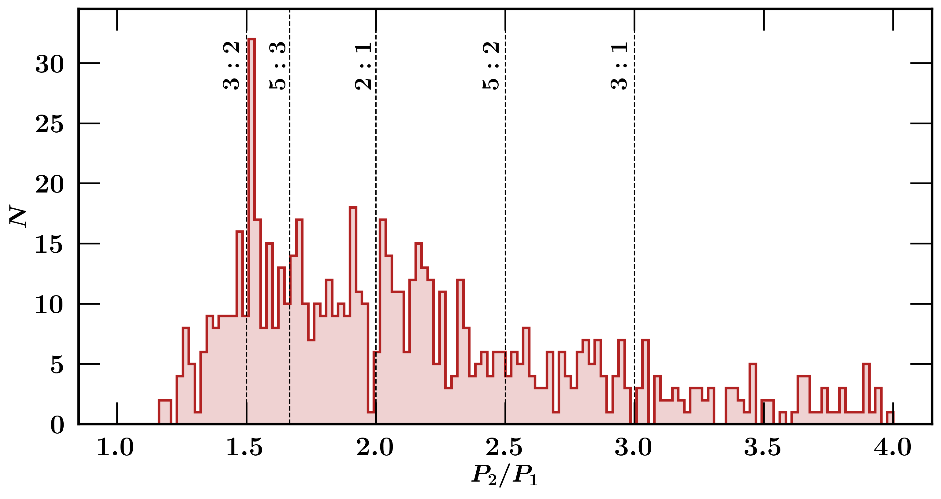
Figure 1: Period ratios $P_{2}/P_{1}$ for all pairs of sub-Neptunes (with radii $<4R_{\oplus}$) in the NASA Exoplanet Archive as of August 1, 2019 ($N$ is the number of systems in a bin). Most sub-Neptunes are not in low-order resonances, but there are excesses of systems (“peaks”) just wide of the 3:2 and 2:1 commensurabilities, and corresponding deficits (“troughs”) just short of these resonances. See Appendix A for how these data separate by host star spectral type.

As revealed by the Kepler mission, sub-Neptunes (planets with radii $\lesssim 4R_{\oplus}$) are a dominant demographic, orbiting an order-unity fraction of all FGKM stars with periods less than a year (e.g., Fressin et al., 2013; Dressing & Charbonneau, 2015; Petigura et al., 2018; Zhu et al., 2018). And where there is one sub-Neptune orbiting a star, there is frequently at least another (e.g., Zhu et al., 2018; Sandford et al., 2019).

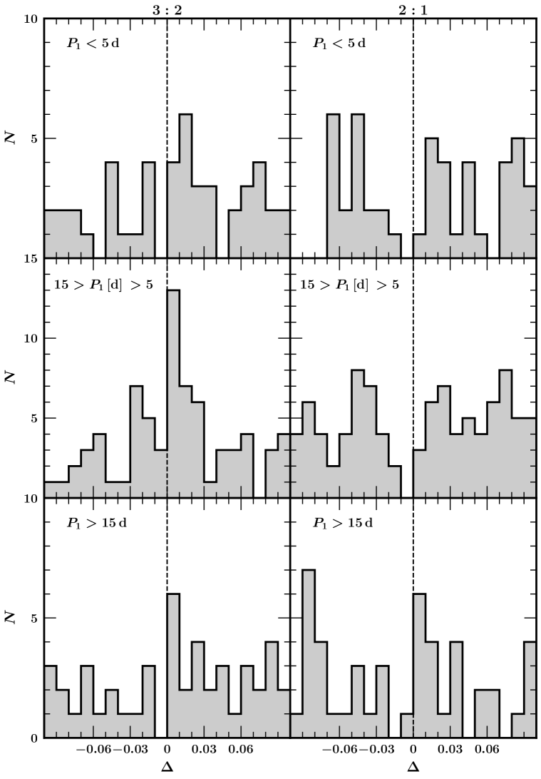
Figure 2: Distribution of $\Delta$, the fractional separation from nominal resonance (equation 1), for observed systems near the 3:2 and 2:1 commensurabilities ($N$ is the number of systems in a bin). This figure is modeled after fig. 2 of Delisle & Laskar (2014) who argued that the excess of systems just wide of resonance—what we call the “peak”—diminishes at large period ($P_{1}>15$ days), apparently implicating tidal interactions with the star which weaken rapidly with increasing orbital distance. However, their figure employs a bin that is centered at $\Delta=0$ and therefore mixes $\Delta<0$ systems with $\Delta>0$ systems, ignoring their qualitatively different dynamics. Correcting the bin boundaries recovers the peak and also its associated trough at all periods, suggesting that tidal effects are not sufficient to explain the asymmetry, especially at large period. Tides might still have a role to play in shifting the peak to larger $\Delta$ at the shortest periods; this trend is stronger for the 2:1 than for the 3:2, as shown further in Figure 3.

Lissauer et al. (2011) and Fabrycky et al. (2014) measured the period ratios $P_{2}/P_{1}$ of neighboring pairs of planets (the subscript 1 denoting the inner member of the pair, and 2 the outer). Figure 1 presents an updated measurement of this period ratio distribution using the NASA Exoplanet Archive. For the most part, the distribution of $P_{2}/P_{1}$ is broadly distributed between $\sim$1.2 and 4, the lower bound marking the boundary of dynamical stability (excepting planets in 1:1 resonance, so far undetected). Superposed on this continuum are excess numbers of planet pairs situated just wide of the 3:2 and 2:1 mean motion commensurabilities. That is, when populations are binned in $P_{2}/P_{1}$, the bins situated just a percent or so larger than 3/2 or 2/1 contain significantly more systems than neighboring bins—there are resonant “peaks” in the histogram. Accompanying these peaks are “troughs”—deficits of planet pairs with period ratios a percent or so smaller than 3/2 or 2/1. Similar substructure might also be present near the second-order 5:3 and 3:1 commensurabilities (see Xu & Lai, 2017). So far as we can tell, these period ratio asymmetries are common to both FGK and M host stars (see Appendix A).

We use the dimensionless parameter

$$\Delta\equiv\frac{q}{q+1}\frac{P_{2}}{P_{1}}-1$$ (1)

to measure the deviation of the (instantaneous) period ratio away from a first-order $(q+1)$:$q$ commensurability. The condition $\Delta=0$ is sometimes called “nominal resonance", a condition not necessarily equivalent to the pair actually being “in resonance” or “resonantly locked”; the latter terms imply that one or more resonant arguments librate (i.e., one or more linear combinations of orbital longitudes oscillate about fixed points; e.g., Murray & Dermott 1999). The peak-trough asymmetry is an excess of planet pairs at $\Delta\sim 0.01$, and a deficit of pairs at $\Delta\sim-0.01$, for $q=1$ and $q=2$.

The preference of resonant systems for $\Delta>0$ can be seen in the circular restricted planar three-body problem. An inner test particle near a $(q+1)$:$q$ resonance with an outer planet of mass $\mu^{\prime}$ relative to the central star obeys the following equations, written here to leading order in the test particle eccentricity and to order-of-magnitude accuracy:

$$\dot{n} \sim\mu^{\prime}en^{2}\sin\phi$$ (2)

$$\dot{e} \sim\mu^{\prime}n\sin\phi$$ (3)

$$\dot{\phi} \sim(q+1)n^{\prime}-qn+\frac{n\mu^{\prime}}{e}\cos\phi$$ (4)

where $\phi=(q+1)\lambda^{\prime}-q\lambda-\varpi$ is the resonant argument, $\lambda$, $\varpi$, $e$, and $n\equiv 2\pi/P$ are the mean longitude, longitude of periapse, eccentricity, and mean motion of the test particle, and primed quantities refer to the outer perturber on a fixed circular orbit. For an inner test particle locked in resonance, $\phi$ librates about the fixed point $\phi_{0}=0$; if the particle resides at the fixed point with zero libration, $\dot{\phi}=0$ and

$$(q+1)n^{\prime}-qn\sim-\frac{n\mu^{\prime}}{e}<0$$ (5)

from which $\Delta>0$ follows. In other words, the inner test particle must speed up its mean motion (relative to nominal resonance) if it is to repeatedly reach conjunction at periapse in the face of apsidal regression; the smaller the eccentricity, the faster the regression, and the more different the particle and perturber mean motions have to be. The same conclusion holds for the case of an outer test particle resonantly locked with an interior perturber. To be locked in a $(q+1)$:$q$ resonance with zero libration is actually to be at a period ratio slighter greater than $(q+1)$:$q$, in the absence of external sources of precession.

When resonantly locked planets have their orbital eccentricities damped by an external agent, they are wedged farther apart in semimajor axis ($\dot{\Delta}>0$; Papaloizou & Terquem 2010; Lithwick & Wu 2012; Batygin & Morbidelli 2013). This “resonant repulsion” can be seen in equation (5), whose right-hand side becomes more negative as $e$ decreases. When eccentricites are damped following a fixed time constant, $\Delta\propto t^{1/3}$ asymptotically. Resonant repulsion has been proposed as a mechanism to transport systems out of the trough at negative $\Delta$ and into the peak at positive $\Delta$.

One way to damp eccentricities and drive repulsion is by dissipating the eccentricity tide raised on planets by their host stars. However, on the face of it, the tidal dissipation rates required to reproduce the observed $\Delta$-distribution within the system age are too large compared to dissipation rates inferred from Solar System planets (Lee et al. 2013; Silburt & Rein 2015; but see Section 6 where we discuss the proposal by Millholland & Laughlin 2019 that dissipation can be provided by obliquity tides). Furthermore, if tides, whose strength diminishes rapidly with increasing distance from the host star, were the sole driver of resonant repulsion, the peak-trough asymmetry should become less pronounced at longer orbital periods. From Figure 2 we are hard pressed to say this is the case, as we can still make out the peak and the trough at periods $\gtrsim 15$ days (cf. Delisle & Laskar 2014 who claimed otherwise, using a non-optimal binning scheme for their fig. 2; see the caption to our Figure 2). Tides might still have a role to play insofar as the peak appears to shift to larger positive $\Delta$ with decreasing period (Delisle & Laskar 2014, their fig. 3); our Figure 3 shows that this trend applies more to the 2:1 than to the 3:2. Our interpretation of these various mixed (and low signal-to-noise) messages is that tidal interactions with the star may have shaped the period ratio asymmetry at the shortest periods, but may not be the whole story, especially at long periods.

Another way to damp eccentricities is by torques exerted on planets by their parent gas discs, during the planet formation era (Goldreich & Tremaine, 1980; Artymowicz, 1993; Cresswell et al., 2007). In addition to damping planet eccentricities, discs also change planet semimajor axes (Goldreich & Tremaine, 1980), i.e., they drive orbital migration, typically toward the star (Ward, 1997; Kley & Nelson, 2012). Planets that migrate convergently (toward smaller $P_{2}/P_{1}$) can become captured into mean-motion resonance. Whether the resonance is stable in the face of continued migration and eccentricity damping depends on the planet masses (Meyer & Wisdom, 2008; Goldreich & Schlichting, 2014; Deck & Batygin, 2015). Sufficiently high planet masses lead to permanent capture, with eccentricity pumping by resonant migration balancing eccentricity damping by the disc (e.g., Lee & Peale, 2002). The equilibrium eccentricities so established imply a positive equilibrium value for $\Delta$ (cf. equation 5) that depends on planet-to-star mass ratios and the relative rates at which the disc drives eccentricity and semimajor axis changes (Terquem & Papaloizou, 2019).

In this paper we ask whether disc-planet interactions can reproduce the observed peak-trough features in the $\Delta$-distribution near first-order resonances. We seek to use the observed period ratio distribution to constrain the extent to which sub-Neptunes migrated, a question tied to how much gas was present in the parent disc around the time these planets finished forming (i.e., completed their last doubling in mass). On the one hand, the observation that most planets neither lie near a period commensurability nor pile up at short periods suggests the majority of systems formed in situ (e.g., Lithwick & Wu, 2012; Lee & Chiang, 2017; Terquem & Papaloizou, 2019; MacDonald et al., 2020), consistent with formation models staged late in a disc’s life, when little gas remains to drive migration (e.g., Kominami & Ida, 2002; Lee & Chiang, 2016; Lee et al., 2018). On the other hand there are gas-rich scenarios for sub-Neptune formation—pebble accretion falls in this category (e.g., Bitsch et al., 2019; Lambrechts et al., 2019; Rosenthal & Murray-Clay, 2019)—where the many systems caught into resonance by disc-driven migration must eventually escape resonance, ostensibly because of instabilities driven by disc eccentricity damping (Goldreich & Schlichting, 2014; Deck & Batygin, 2015) or chaos in high-multiplicity systems (Pu & Wu, 2015; Izidoro et al., 2017, 2019). Our goal is to help decide the in-situ vs. migration (gas-poor vs. gas-rich disc) debate for sub-Neptunes by quantifying the disc gas surface density and the extent of planet-disc interaction needed to reproduce the peak-trough asymmetry revealed by ${\it Kepler}$.

We begin in Section 2 by laying out the equations of motion solved in this paper for near-resonant, disc-driven pairs of planets. In Section 3 we review, for the special case of the circular restricted planar three-body problem, the behaviour of near-resonant test particles whose semi-major axes and eccentricities are externally driven by a disc. There we survey the various possible evolutions for $\Delta$. Section 4 describes how these results are modified when the masses of both planets are accounted for. Our main contribution is in Section 5 where we carry out a population synthesis, generating mock populations of planet pairs that evolve under the influence of a disc, and comparing our calculated $\Delta$-distributions to the observed $\Delta$-distribution to constrain disc properties. In Section 6 we place our results in the context of our understanding of planet formation and identify areas for future work.

By design our paper studies planet-disc interactions and does not model stellar tidal interactions. Most of our calculations (all those in Sections 4–5) will be for the 3:2 resonance, which exhibits the strongest peak-trough asymmetry and the one least sensitive to distance from the host star (Figures 1–3). Our hypothesis is that 3:2 systems are least impacted by tides. We bring the 2:1 resonance back into consideration in Section 6. There we assess the extent to which disc-planet interactions, which establish a baseline for the peak-trough asymmetry, need to be abetted by tides.

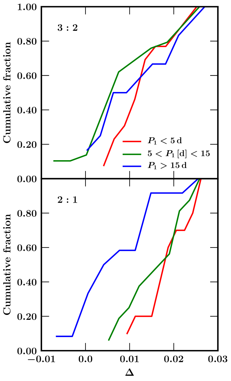
Figure 3: Similar to Figure 2, but now plotting the cumulative distribution function, which is not sensitive to choice of bins. This figure confirms the trend reported by Delisle & Laskar (2014, their fig. 3) that planet pairs situated closer to the host star have larger $\Delta$ than those situated farther away, and shows further that this behaviour is stronger for the 2:1 resonance than for the 3:2.

2 Equations of Motion

To leading order in eccentricity, two planets of mass $m_{1}$ and $m_{2}$ orbiting a star of mass $M_{\star}$ near a $(q+1)$:$q$ mean motion resonance obey the following coupled ordinary differential equations for their mean motions $n$, eccentricities $e$, and resonant arguments $\phi$ (subscript 1 for the inner planet and 2 for the outer planet; e.g., Terquem & Papaloizou 2019):

$$\dot{n}_{1} =-3qn_{1}^{2}\frac{\alpha m_{2}}{M_{\star}}\left(e_{1}f_{1}\sin\phi_{1}+e_{2}f_{2}\sin\phi_{2}\right)$$

$$+\frac{3n_{1}}{2t_{a,1}}+\frac{pn_{1}e_{1}^{2}}{t_{e,1}}$$ (6)

$$\dot{n}_{2} =3(q+1)n_{2}^{2}\frac{m_{1}}{M_{\star}}\left(e_{1}f_{1}\sin\phi_{1}+e_{2}f_{2}\sin\phi_{2}\right)$$

$$+\frac{3n_{2}}{2t_{a,2}}+\frac{pn_{2}e_{2}^{2}}{t_{e,2}}$$ (7)

$$\dot{e}_{1} =-n_{1}\frac{\alpha m_{2}}{M_{\star}}f_{1}\sin\phi_{1}-\frac{e_{1}}{t_{e,1}}$$ (8)

$$\dot{e}_{2} =-n_{2}\frac{m_{1}}{M_{\star}}f_{2}\sin\phi_{2}-\frac{e_{2}}{t_{e,2}}$$ (9)

$$\dot{\phi}_{1} =(q+1)n_{2}-qn_{1}-n_{1}\frac{\alpha m_{2}}{M_{\star}}\frac{1}{e_{1}}f_{1}\cos\phi_{1}$$ (10)

$$\dot{\phi}_{2} =(q+1)n_{2}-qn_{1}-n_{2}\frac{m_{1}}{M_{\star}}\frac{1}{e_{2}}f_{2}\cos\phi_{2}\,.$$ (11)

The coefficients $f_{1}$ and $f_{2}$ are given in terms of the ratio of semimajor axes $\alpha\equiv a_{1}/a_{2}$ and Laplace coefficients:

$$f_{1}=-\frac{1}{2}\left[2(q+1)+\alpha\frac{d}{d\alpha}\right]b_{1/2}^{q+1}(\alpha)$$ (12)

$$f_{2}=\frac{1}{2}\left[2q+1+\alpha\frac{d}{d\alpha}\right]b_{1/2}^{q}(\alpha)-2\alpha\delta_{q,1}$$ (13)

$$b_{1/2}^{j}(\alpha)=\frac{1}{\pi}\int_{0}^{2\pi}\frac{\cos(j\psi)}{\left(1-2\alpha\cos\psi+\alpha^{2}\right)^{1/2}}d\psi$$ (14)

where $\delta_{q,1}$ is the Kronecker $\delta$.

We focus on the case $q=2$, i.e., the $n_{1}$:$n_{2}$ = 3:2 resonance for which the observed peak-trough asymmetry is strongest and least sensitive to orbital distance (read: least affected by stellar tidal interactions; Figures 1–3). We hold fixed $f_{1}=-2.025$ and $f_{2}=2.484$, the values appropriate for $\alpha=a_{1}/a_{2}=(2/3)^{2/3}$ at nominal resonance. In reality, $\alpha$ varies with time, but by amounts too small for the resultant changes to $f_{1}$ and $f_{2}$ to matter.

To the resonant interaction terms (those depending on $\phi$ in equations 6–9) we have added terms for semi-major axis and eccentricity damping by an external agent—in this paper, the disc—parameterized by the timescales $t_{a}$ and $t_{e}$. The coefficient $p$ measures the extent to which eccentricity damping alone (ignoring the resonant potential) produces semi-major axis changes. If eccentricity damping alone conserved a planet’s orbital angular momentum, then $p=3$. Although disc torques (first-order co-orbital Lindblad torques in the case of eccentricity damping; e.g., Duffell & Chiang 2015 and references therein) generally do not conserve the planet’s angular momentum, the relevant value of $p$ may differ from 3 only by an order-unity factor. Moreover, both resonant repulsion (Lithwick & Wu, 2012) and resonant equilibria (Goldreich & Schlichting, 2014; Terquem & Papaloizou, 2019) are not too sensitive to $p$ (which could even be 0). For simplicity, and following previous work, we adopt $p=3$. Note further that the effect of the disc on apsidal precession has been neglected; the last terms in equations (10) and (11) account only for precession due to the resonance.

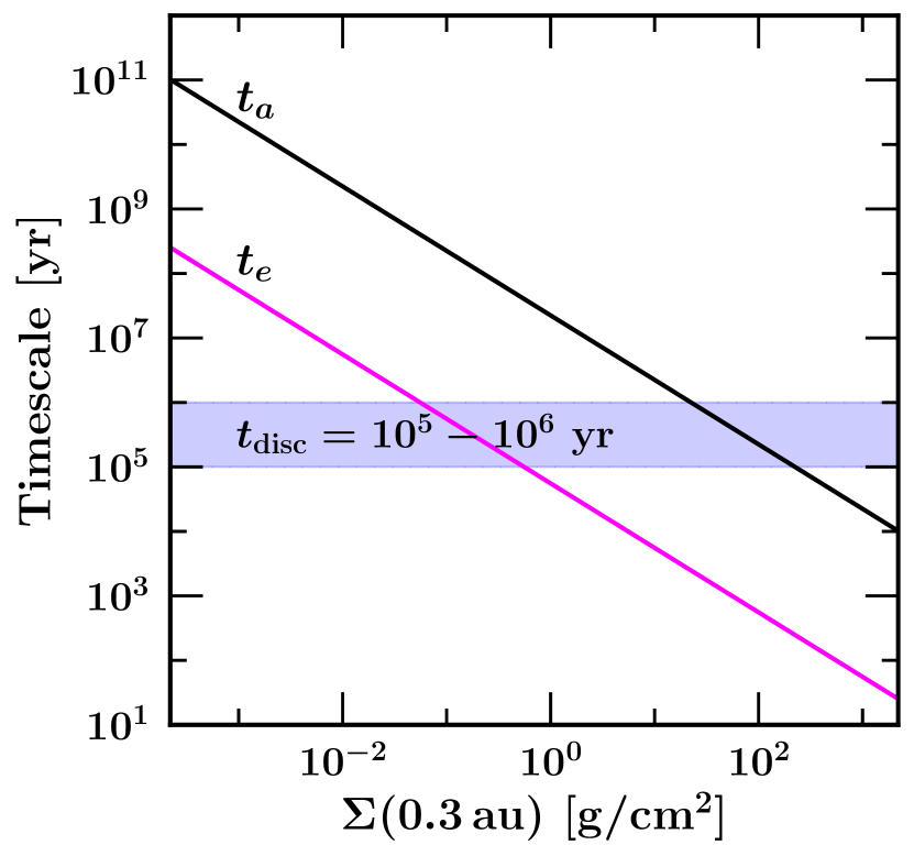
Figure 4: Characteristic semi-major axis and eccentricity damping times $t_{a}=a/|\dot{a}|$ and $t_{e}=e/|\dot{e}|$ for a sub-Neptune in a disc, as a function of the disc gas surface density $\Sigma$, evaluated for a planet mass of $10\,M_{\oplus}$ and an orbital radius of $a=0.3$ au. The shaded region indicates possible disc dispersal (e-folding) timescales. Eccentricity damping by the disc is faster than semi-major axis damping (orbital migration) by a factor of order $(a/h)^{2}$.

For the semi-major axis damping time $t_{a}$ we utilize the numerically calibrated value of Kley & Nelson (2012):

$$t_{a}=\frac{m\sqrt{GM_{\star}a}}{2|\Gamma|}$$ (15)

$$\Gamma=-\left(1.36+0.62\beta_{\Sigma}+0.43\beta_{T}\right)\left(\frac{m}{M_{\star}}\right)^{2}\left(\frac{h}{a}\right)^{-2}\Sigma a^{4}\Omega^{2}$$ (16)

where $G$ is the gravitational constant, and $\Sigma$, $h/a$, and $\Omega$ are the disc surface density, aspect ratio, and Keplerian angular frequency evaluated at the planet’s semimajor axis $a$, respectively. The variables $\beta_{T}\equiv-d\log T/d\log a$ and $\beta_{\Sigma}\equiv-d\log\Sigma/d\log a$ are the power-law indices describing how temperature and surface density vary with disc radius. We assume $\beta_{T}=3/7$ (Chiang & Goldreich, 1997) and set

$$h/a=0.04\left(\frac{a}{1\,{\rm au}}\right)^{2/7}\,.$$ (17)

For most of our calculations we choose for simplicity $\beta_{\Sigma}=0$. A flat $\Sigma$ profile yields nearly equal fractions of convergently and divergently migrating planet pairs, assuming $m_{2}$ and $m_{1}$ are drawn independently from the same distribution. However, we also experiment with $\beta_{\Sigma}$ up to 3/2 (the value appropriate to the minimum-mass solar and extrasolar nebulas; Chiang & Laughlin 2013). We assume $\Sigma$ decays exponentially with time:

$$\Sigma(a,t)=\Sigma_{0}\left(\frac{a}{1\,{\rm au}}\right)^{-\beta_{\Sigma}}\exp(-t/t_{\rm disc})$$ (18)

with a nominal $t_{\rm disc}=10^{5}$ yr, arguably appropriate for the innermost regions of discs where Kepler sub-Neptunes reside (e.g., Alexander et al., 2014). The initial surface density normalization $\Sigma_{0}$ is a free parameter that we will fit to the observations (Section 5).

The eccentricity damping timescale is given by

$$t_{e}=\left(\frac{M_{\star}}{m}\right)\left(\frac{M_{\star}}{\Sigma a^{2}}\right)\left(\frac{h}{a}\right)^{4}\Omega^{-1}$$ (19)

(e.g., Kominami & Ida 2002). There are corrections to $t_{e}$ that grow with $e/(h/a)$ (Papaloizou & Larwood, 2000), but these are less than order-unity for the small eccentricities considered here and are therefore omitted (cf. Xu et al., 2018). Figure 4 plots sample values of $t_{a}$ and $t_{e}$ as a function of $\Sigma$, for $a=0.3$ au and $m=10\,M_{\oplus}$. For our disc parameters, the ratio $t_{a}/t_{e}$ for a single planet varies from 200 to 750 as $a$ varies from 1 au to 0.1 au.

The migration we model is smooth and of varying rates depending on the gas surface density. Rein (2012) also study near-resonant planets torqued by discs, but focus on stochastic migration in turbulent, gas-rich discs. Their model employs a fixed value for the ratio of damping timescales $t_{a}/t_{e}=10$ that appears underestimated by more than an order of magnitude.

Equations (6)–(11) are solved numerically for how the distance from period commensurability $\Delta$ evolves for a pair of planets embedded in a decaying disc. We carry out all numerical integrations using the lsoda package, enforcing a fractional tolerance of $10^{-10}$ on the accuracy of our solutions. As a check on our calculations, we compared them against analytic equilibrium solutions for $e_{1}$, $e_{2}$, and $\Delta$ as derived by Terquem & Papaloizou (2019; their equations 35, 36, and 49):

$$e_{\rm eq,1} =\left\{\frac{t_{e,1}/t_{a,2}-t_{e,1}/t_{a,1}}{2\left(q+1\right)\left(1+\frac{q}{q+1}\frac{m_{1}}{\alpha m_{2}}\right)\left[1+\frac{m_{1}}{\alpha m_{2}}\left(\frac{q}{q+1}\right)^{2}\left(\frac{f_{2}}{f_{1}}\right)^{2}\frac{t_{e,1}}{t_{e,2}}\right]}\right\}^{1/2}$$ (20)

$$e_{\rm eq,2} =e_{\rm eq,1}\left(\frac{m_{1}}{\alpha m_{2}}\right)\left(\frac{q}{q+1}\right)\left|\frac{f_{2}}{f_{1}}\right|$$ (21)

$$\Delta_{\rm eq} =\sqrt{-\mathcal{A}/\mathcal{B}}$$

$$\mathcal{A} =\frac{3}{q^{2}t_{e,1}}\left(\frac{q}{q+1}\frac{m_{1}}{\alpha m_{2}}+1\right)\left(\frac{\alpha m_{2}}{M_{\star}}\right)^{2}\times$$

$$\left[(q+1)f_{1}^{2}+\frac{q^{2}}{q+1}\frac{m_{1}}{\alpha m_{2}}f^{2}_{2}\frac{t_{e,1}}{t_{e,2}}\right]>0$$

$$\mathcal{B} =\frac{3}{2t_{a,1}}\left(1-\frac{t_{a,1}}{t_{a,2}}\right)<0\,.$$ (22)

Application of equations (20)–(22) is restricted to the case where a pair of planets migrate convergently (so $\mathcal{B}<0$, either because (i) $t_{a,1}/t_{a,2}>1$ for $t_{a,1},t_{a,2}>0$, (ii) $t_{a,1}<0$ and $t_{a,2}>0$, or (iii) $t_{a,1}/t_{a,2}<1$ for $t_{a,1},t_{a,2}<0$) and locked in mutual resonance (at $\cos\phi_{1}=1$ and $\cos\phi_{2}=-1$). Our numerical solutions to the more general equations (6)–(11) do not make these assumptions.

Some additional notes on the validity of equations (6)–(11): the terms depending on $\phi$ reasonably describe the interaction potential “near resonance”, meaning either when $\phi$ is librating about a fixed value (in resonance), or when $\phi$ is circulating from $0$ to $2\pi$ outside and not too far from resonance (see, e.g., Murray & Dermott 1999, their figure 8.16, panels e and f). Far from resonance, keeping these terms and neglecting other short-period terms is technically not accurate, but the error is of little consequence, as here all terms depending on mean longitudes time-average to zero anyway. For our model parameters, the planets are never situated so far from resonance that their forced eccentricities (forced by the resonance) are smaller than the forced eccentricities from other short-period terms; the former are of order $\mu/\Delta$, where $\Delta<0.1$ for all calculations in this paper, while the latter are of order $\mu$ (Agol et al. 2005, their section 5). These eccentricities, and our modeled eccentricities which by assumption start at values $<0.1$ and decrease by disc damping, are all small enough that a first-order expansion of the resonance potential suffices.

3 The Restricted Problem

Case	Test particle	$\mu$	$|t_{a}|/t_{e}$	Migration	$\phi_{\rm final}$	Resonant repulsion?	$\Delta_{\rm final}$	$e_{\rm final}$
1	Inner	Any	$\infty$	None	0+	Yes	$\Delta_{\rm eq}=\infty$	0
2	Inner	$>\mu_{\rm crit}$	100	Convergent	0+	Yes	$\Delta_{\rm eq}$	$e_{\rm eq,1}$
3	Inner	$<\mu_{\rm crit}$	100	Convergent	$\pi^{-}$	No	$\ll\Delta_{\rm initial}$	0
4	Inner	Any	100	Divergent	$0^{+}$	No	$\gg\Delta_{\rm initial}$	0
5	Outer	Any	$\infty$	None	$\pi^{+}$	Yes	$\Delta_{\rm eq}=\infty$	0
6	Outer	Any	100	Convergent	$\pi^{+}$	Yes	$\Delta_{\rm eq}$	$e_{\rm eq,2}$
7	Outer	Any	100	Divergent	$\pi^{+}$	No	$\gg\Delta_{\rm initial}$	0

Table 1: Summary of the behaviour of a test particle in the restricted planar circular three-body problem near the 3:2 resonance, when the test particle’s eccentricity is damped and when its semi-major axis is driven either outward or inward. Columns specify: (1) case number, (2) whether the test particle resides interior or exterior to the perturber (“Inner” vs. “Outer”), (3) the perturber-to-star mass ratio, with the value $\mu_{\rm crit}$ (above which resonance capture is permanent and below which it is not) given by equation (28) of Goldreich & Schlichting (2014), (4) the ratio of the externally imposed e-folding timescales for the test particle semi-major axis and eccentricity, where $\infty$ denotes infinite $t_{a}$ and finite $t_{e}$, (5) whether migration is convergent or divergent (as controlled by the sign of $t_{a}$) or is not imposed, (6) the late-time value of the test particle’s resonant angle $\phi$, with superscripts “+” and “-” denoting values slightly greater or less than the listed number, (7) whether or not the planet-particle pair exhibits resonant repulsion, (8) the late-time value of the pair’s distance from nominal resonance $\Delta$, with equilibrium values $\Delta_{\rm eq}$ given by equations (23) and (25), (9) the late-time value of the eccentricity, with equilibrium values $e_{\rm eq}$ given by equations (24) and (26). Cases 1, 2, 5, and 6 can lead to permanent capture into resonance; cases 3, 4, and 7 cannot.

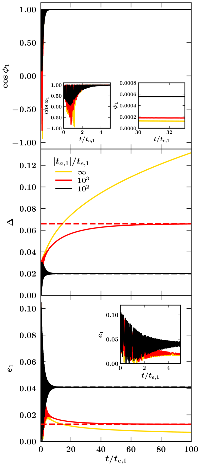
Figure 5: Evolution of an inner test particle whose semi-major axis and eccentricity are externally driven, near the 3:2 resonance with an outer massive perturber having $\mu=10^{-3}$ on a fixed circular orbit. The test particle is captured into resonance ($\phi_{1}$ locks to a stable point slightly greater than 0; top panel) either by eccentricity damping operating alone (yellow curves), or a combination of eccentricity damping and convergent migration (red and black curves). In the former case, the test particle eccentricity $e_{1}$ asymptotes to zero (bottom panel) and the separation $\Delta$ from nominal resonance increases as $t^{1/3}$ (middle panel; Lithwick & Wu 2012; Batygin & Morbidelli 2013). When convergent migration is added, resonant amplification of eccentricity balances disc eccentricity damping to yield an equilibrium eccentricity $e_{\rm eq,1}$ and an equilibrium separation $\Delta_{\rm eq}$; their values calculated analytically from equations (20) and (22) are shown as dashed lines and agree with our numerical results.

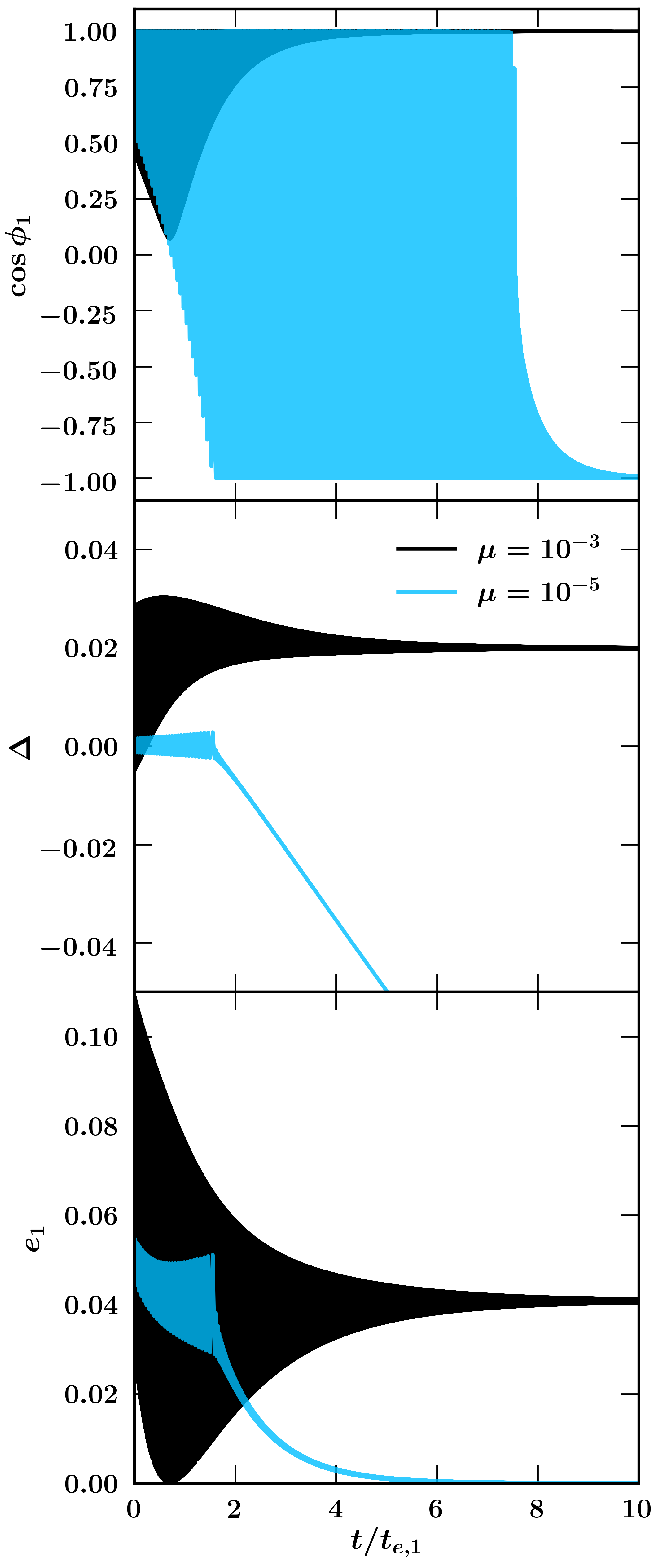
Figure 6: Same as Figure 5 but for fixed $|t_{a,1}|/t_{e,1}=100$ and two perturber-to-star mass ratios $\mu$. For low $\mu$ the inner test particle experiences overstable librations and eventually escapes resonance (blue curve).

To gain intuition and connect to previous work, we first explore the restricted problem where one of the planets is replaced with a test particle, while the other planet of non-zero mass $m\equiv\mu M_{\star}$ is kept on a fixed circular orbit (in this section we forgo the primed vs. unprimed notation). The damping timescales $t_{a}$ and $t_{e}$ refer here to the test particle, and are held constant in a given integration for simplicity (they do not refer to a depleting disc per se). We explore both the cases of an inner test particle ($m_{1},e_{2}\rightarrow 0$ and $t_{a,2},t_{e,2}\rightarrow\infty$ in equations 6-11) and outer test particle ($m_{2},e_{1}\rightarrow 0$, $t_{a,1},t_{e,1}\rightarrow\infty$), as well as both convergent and divergent migration (controlled by the sign of $t_{a}$ which we allow here to be negative). For the integrations reported in this section, initial conditions are as follows: $\Delta_{\rm initial}=0$, test particle $\phi_{\rm initial}=1$ rad (away from the fixed points of the resonance near 0 and $\pi$), and test particle $e_{\rm initial}=0.05$. Other initializations give qualitatively similar outcomes.

We begin with the case where an inner test particle is subject only to eccentricity damping ($t_{e,1}$ finite, $t_{a,1}=\infty$). From Figure 5, made for an outer perturber of mass $\mu=10^{-3}$, we see the test particle lock into resonance on a timescale of order $t_{e,1}$ (top panel, left inset). The resonant angle $\phi_{1}$ settles to a small positive value (top panel, right inset). This small offset in $\phi_{1}$ away from 0 (the dissipationless equilibrium point) arises because eccentricity damping accelerates apsidal regression ($\dot{\varpi}_{1}\propto-1/e_{1}$), causing conjunctions to occur just after periapse. Such conjunctions remove angular momentum from the test particle (e.g., Peale 1986), driving it away indefinitely according to $\Delta\propto t^{1/3}$ (middle panel, yellow curve). Lithwick & Wu (2012) term this behaviour resonant repulsion—the bodies, locked in resonance, are repelled farther apart.

Figure 5 also shows that for convergent migration at finite $t_{a,1}<0$ ($|t_{a,1}|$ is allowed to vary from $10^{2}t_{e,1}$ to $10^{3}t_{e,1}$) the planet-particle pairs do not wedge apart for all time but reach an equilibrium separation $\Delta_{\rm eq}>0$, i.e., they reach an equilibrium wide of resonance. From equation (missing) 22,

$$\Delta_{\rm eq}=-\frac{\alpha\mu f_{1}}{q}\sqrt{2(q+1)\frac{|t_{a,1}|}{t_{e,1}}}>0$$ (23)

which agrees with our numerical results (middle panel). This equilibrium $\Delta_{\rm eq}$ corresponds to an equilibrium eccentricity $e_{\rm eq,1}$ (given by equation A1 of Goldreich & Schlichting 2014, or our equation 20 taken from Terquem & Papaloizou 2019; see also equation 5). The equilibrium eccentricity reflects the balance between eccentricity pumping by resonant migration (driven by $t_{a,1}$) and eccentricity damping by the disc ($t_{e,1}$):

$$e_{\rm eq,1}=\sqrt{\frac{1}{2(q+1)}\frac{t_{e,1}}{|t_{a,1}|}}$$ (24)

which also matches our numerical results (bottom panel).

The value of $\mu=10^{-3}$ in Figure 5 was chosen to exceed $\mu_{\rm crit}\propto(t_{e,1}/|t_{a,1}|)^{3/2}$, the value above which the resonance is stable to eccentricity damping and below which it is not; we find using equation (28) of Goldreich & Schlichting (2014) that $\mu_{\rm crit}\simeq 6\times 10^{-5}$ for $|t_{a,1}|/t_{e,1}=10^{2}$. In Figure 6 we verify that for a lower perturber mass, $\mu=10^{-5}$, the test particle eventually escapes resonance after a few $t_{e,1}$, after which its eccentricity decays exponentially to zero, and $\Delta$ becomes increasingly negative because of the imposed convergent migration (i.e., equation 6 reduces to $\dot{n}_{1}=3n_{1}/(2t_{a,1})$).

The behaviours discussed so far for the inner test particle are summarized as cases 1, 2, and 3 in Table 1. Divergent migration for the inner test particle, case 4, does not lead to permanent resonance capture (e.g., Murray & Dermott, 1999) and simply causes $\Delta$ to increase on timescale $t_{a,1}$. Table 1 also provides entries for an outer test particle. An outer test particle behaves similarly to an inner test particle, except that all perturber masses can permanently capture an outer test particle when migration is convergent (contrast cases 2 and 3 for the inner test particle with the single case 6 for an outer test particle; see also section 2.2.2 of Deck & Batygin 2015). When an outer test particle migrates convergently and is resonantly captured, the equilibrium separation and eccentricity are given by the appropriate limits of equations (20)–(22):

$$\Delta_{\rm eq}=\frac{\mu f_{2}q}{q+1}\sqrt{\frac{2}{q}\frac{t_{a,2}}{t_{e,2}}}>0$$ (25)

$$e_{\rm eq,2}=\sqrt{\frac{1}{2q}\frac{t_{e,2}}{t_{a,2}}}\,.$$ (26)

4 The unrestricted problem

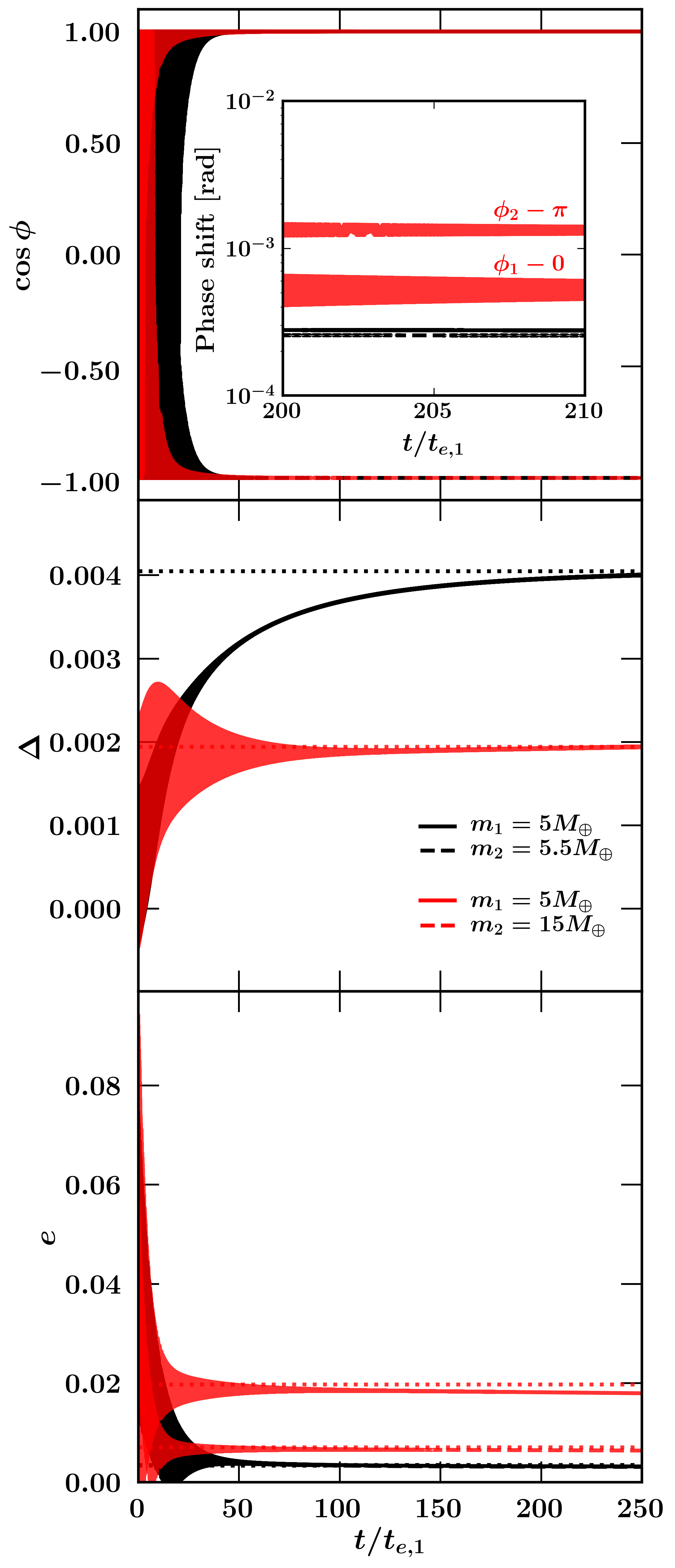
Figure 7: Analogous to Figure 5, but for convergently migrating planet pairs with non-zero masses (lifting the test particle restriction). Two sets of mass pairings are considered (black vs. red curves). Initial conditions for both sets are as follows: $e_{\rm 1,initial}=e_{\rm 2,initial}=0.05$, $\phi_{\rm 1,initial}=1$ rad, $\phi_{\rm 2,initial}=2$ rad, $a_{\rm 1,initial}=0.3$ au, and $\Delta_{\rm initial}=0$. We use our fiducial disc parameters except that we fix $\Sigma=10$ g/cm² for simplicity (we do not let the disc decay) and terminate the integration when $t/t_{e,1}=250$. At this end time, we analytically evaluate equilibrium values $\Delta_{\rm eq}$, $e_{\rm eq,1}$, and $e_{\rm eq,2}$ using equations (20)–(22), and plot them as horizontal dotted lines in the middle and bottom panels. The behaviours seen here for the unrestricted problem are essentially the same as in Figure 5 for the restricted problem: the bodies lock into resonance ($\phi_{1}$ to $0^{+}$ and $\phi_{2}$ to $\pi^{+}$), and the relative separation $\Delta$ and eccentricities $e_{1}$ and $e_{2}$ equilibrate as expected.

Solutions to the unrestricted problem where both planets have non-zero mass and are torqued by the disc are qualitatively similar to those in the restricted case. Figure 7 displays sample evolutions of two such pairs that convergently migrate and capture into mutual resonance, with $\phi_{1}$ and $\phi_{2}$ driven to values near 0 and $\pi$, respectively. Both pairs attain equilibrium eccentricities and separations that agree with those calculated analytically from equations (20)–(22).

Figure 8 explores how the stability of the resonance changes when going from the restricted to the unrestricted problem. We plot $\mu_{\rm crit}$, the combined planet-to-star mass ratio above which a convergently migrating pair can stay captured in resonance (equation 21 of Deck & Batygin 2015), vs. $m_{1}/m_{2}$ at fixed $m_{1}+m_{2}$. The requirement for stability is easier to satisfy ($\mu_{\rm crit}$ is smaller) in the unrestricted regime where $m_{1}/m_{2}$ is near unity. The variation in $\mu_{\rm crit}$ arises mostly from its dependence on $t_{a}=t_{a,1}t_{a,2}/(t_{a,1}-t_{a,2})$, the relative migration timescale. As the planets become more comparable in mass, their individual timescales for migration $t_{a,1}$ and $t_{a,2}$ approach each other, $t_{a}$ increases, and by extension $\mu_{\rm crit}\propto 1/t_{a}^{3/2}$ decreases. This effect helps to stabilize the population of sub-Neptunes we mock up in Section 5.

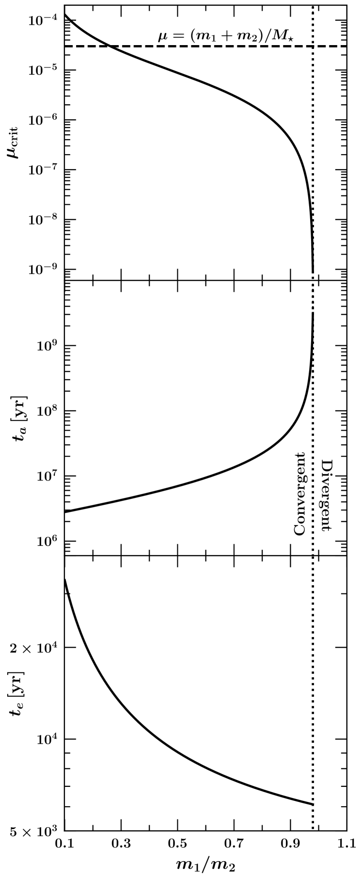
Figure 8: At fixed $m_{1}+m_{2}=10M_{\oplus}$ and fixed $M_{\star}=1M_{\odot}$, the stability of the resonance depends on how mass is distributed between $m_{1}$ and $m_{2}$. The top panel shows the combined planet-to-star mass ratio $\mu_{\rm crit}$ (solid curve) above which resonance capture is permanent and below which it is not, computed from equation (21) of Deck & Batygin (2015) for the 3:2 resonance using our fiducial disc parameters at $a=0.3$ au. As $m_{1}/m_{2}$ increases toward unity, $\mu_{\rm crit}$ decreases, i.e., the threshold for stability is easier to satisfy as we transition from the restricted to the unrestricted three-body problem. The critical value $\mu_{\rm crit}$ scales as $(t_{e}/t_{a})^{3/2}$, where $t_{a}$ is the timescale for relative migration ($1/t_{a}=1/t_{a,2}-1/t_{a,1}$, middle panel) and $t_{e}$ is a weighted average of $t_{e,1}$ and $t_{e,2}$ ($1/t_{e}=1/t_{e,1}+(m_{1}/m_{2})/t_{e,2}$, lower panel). Most of the variation in $\mu_{\rm crit}$ stems from $t_{a}$, which diverges as $m_{1}$ approaches $m_{2}$ (for $m_{1}>0.97m_{2}$, migration is divergent and permanent capture is not possible).

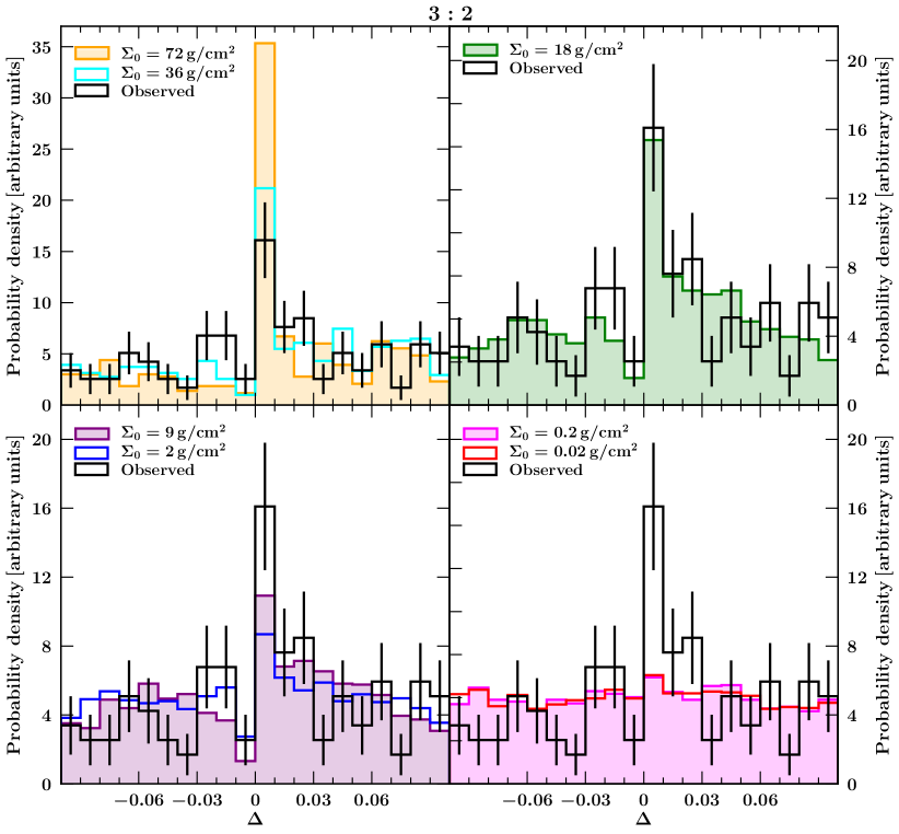
Figure 9: Final distributions of $\Delta$ from our Monte Carlo population synthesis model of the 3:2 resonance (open and filled coloured histograms) compared against the observed distribution (black open histogram). The 3:2 observations are culled of pairs with inner planet periods $P_{1}<5$ days to avoid potential contamination from stellar tidal interactions; see Figures 2 and 3. Of the models shown, the one corresponding to an initial disc gas surface density of $\Sigma_{0}=18$ g/cm² (upper right in green) reproduces the observed peak-trough feature best. This surface density, which characterizes our model disc from 0.1 to 1 au, is 3–4 orders of magnitude lower than corresponding surface densities in minimum-mass, solar-composition reconstructions of protoplanetary discs derived from Kepler data (e.g., Chiang & Laughlin 2013). In our model, the peak mostly comprises planet pairs that convergently migrate from $\Delta_{\rm initial}>0.01$ to an equilibrium separation $\Delta_{\rm eq}\simeq 0.001$–0.01. Values for $\Sigma_{0}\gtrsim 18$ g/cm² lead to more migration and overpredict the number of systems captured into the peak; conversely, $\Sigma_{0}\lesssim 18$ g/cm² underpredicts the peak.

5 Population synthesis

Having reconnoitered the outcomes of two planets undergoing semimajor axis and eccentricity changes near resonance, we now construct a population synthesis model designed to reproduce the observed distribution of $\Delta$’s near the 3:2 resonance. The goal is to identify the disc conditions—in particular the disc gas surface density around the time sub-Neptunes attain their final masses—that are compatible with the $\Delta$-distribution, and thereby assess the degree to which planets migrated. As our model is simplistic, the most we can hope for is that our inferences will be accurate enough to point us in the right direction when thinking about sub-Neptune formation—whether to a gas-rich disc where such planets typically migrate large distances, or to a gas-poor one where they spawn more-or-less in situ.

5.1 Monte Carlo method

Our calculation of the dynamical evolution of a pair of sub-Neptunes begins just after they form, i.e., just after their solid cores, which dominate their masses, coagulate. At this time ($t=0$), the disc gas surface density $\Sigma$ everywhere equals $\Sigma_{0}$ (assuming $\beta_{\Sigma}=0$); thereafter, $\Sigma$ decays exponentially (equation 18). We consider values for $\Sigma_{0}$ between 0.01 and 100 g/cm², a range that we will see brackets the best fit to the observations. For every value of $\Sigma_{0}$ chosen, we integrate the equations of motion (6)–(11) until $\Sigma$ has decreased by two orders of magnitude relative to its initial value. Thus, for example, a model with $\Sigma_{0}=10$ g/cm² is integrated from $\Sigma=10$ g/cm² to $\Sigma=0.1$ g/cm². We have verified that integrating further changes our results negligibly.

For every $\Sigma_{0}$, we construct $N=2000$ planetary systems with properties and initial conditions chosen randomly as follows. Host stellar masses are drawn uniformly from 0.5 to 2 $M_{\odot}$, approximately matching the range of masses reported in the NASA Exoplanet Archive. For every star we lay down two planets whose masses are each drawn randomly from a uniform distribution between 5 and 15 $M_{\oplus}$ (cf. Lithwick et al. 2012; Weiss & Marcy 2014; Hadden & Lithwick 2014, 2017; Wu 2019). The inner planet is initialized with a semimajor axis $a_{\rm 1,initial}$ chosen randomly from a distribution that is uniform in $\log a_{\rm 1,initial}$ between 0.1 and 1 au (corresponding to orbital periods of $\sim$10 to $\sim$400 days); such a distribution is similar to that observed (e.g., Fressin et al., 2013; Dressing & Charbonneau, 2015). We set the outer planet’s semi-major axis such that the pair are near commensurability: we draw $\Delta_{\rm initial}$ from a flat distribution between -0.1 and 0.1, a range that encompasses the observed period ratio asymmetry (e.g., Figure 2). Together, $\Delta_{\rm initial}$ and $a_{\rm 1,initial}$ specify the initial location of the outer planet:

$$a_{\rm 2,initial}=\left[\left(\Delta_{\rm initial}+1\right)\frac{q+1}{q}\right]^{2/3}a_{\rm 1,initial}$$ (27)

with $q=2$ for the 3:2 resonance. Initial eccentricities $e_{\rm 1,initial}$ and $e_{\rm 2,initial}$ are each drawn randomly from a uniform distribution between 0 and 0.1, and initial resonant arguments $\phi_{\rm 1,initial}$ and $\phi_{\rm 2,initial}$ are each drawn randomly from a uniform distribution between 0 and $2\pi$. In general the planets do not begin in resonance.

The semimajor axis and eccentricity driving terms from the background disc are given by equations (15)–(19). They and our input parameters—in particular our nominal choice for $\beta_{\Sigma}=0$—are such that while all planets migrate inward, about 50% of planet pairs convergently migrate ($t_{a,2}<t_{a,1}$), with the remaining fraction migrating divergently. Only a convergent pair can capture into resonance and attain an equilibrium separation $\Delta_{\rm eq}>0$ (see equation 22, and Sections 3 and 4).

For every $\Sigma_{0}$, we compare the $N=2000$ final values of $\Delta$ ($=\Delta_{\rm final}$) against the observed $\Delta$-distribution. Should a planet migrate to the inner edge of the disc, which we take to lie at $P=3$ days (e.g., Lee & Chiang, 2017), we shut off the disc torque acting on the planet, setting its $t_{a}$ and $t_{e}$ to infinity. An inner planet so stopped at the edge may be pushed further inward by resonant interaction with the outer planet; this process stops once the outer planet also hits the disc inner edge, at which point we terminate the integration. We also halt an integration if both planets convergently migrate such that their semimajor axes coincide ($\Delta$ near -1/3). For the models that best fit the observations, none of these eventualities is significant.

5.2 Comparison to observations

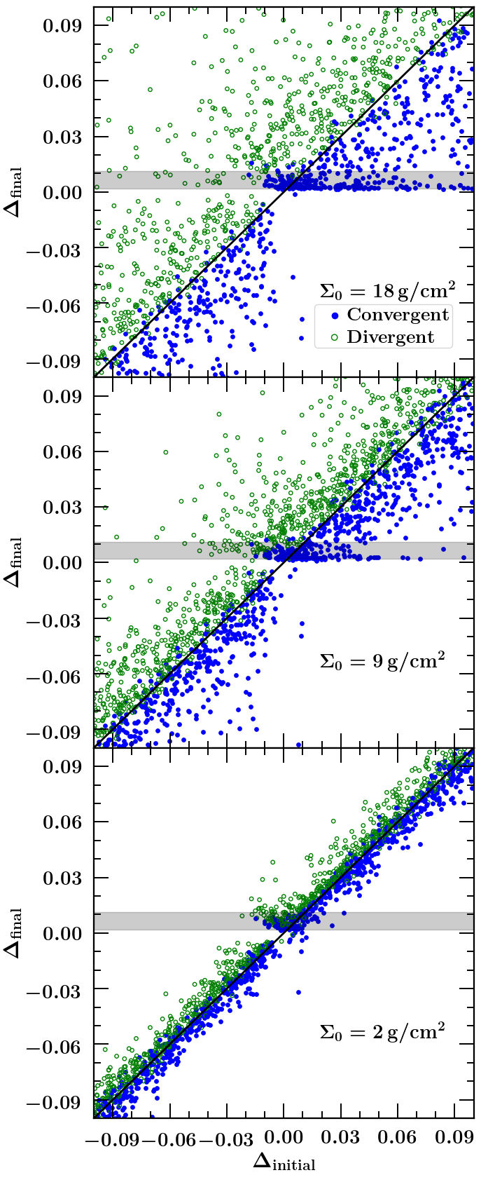
Figure 10: How initial separations $\Delta_{\rm initial}$ map to final separations $\Delta_{\rm final}$, for three population synthesis models with varying initial disc surface densities $\Sigma_{0}$. Away from resonance, convergently migrating pairs (blue points) move down, below the slope 1 line, to $\Delta_{\rm final}<\Delta_{\rm initial}$; divergently migrating pairs (green points) move up to $\Delta_{\rm final}>\Delta_{\rm initial}$. The greater is $\Sigma_{0}$ (the more massive the disc), the more systems move in $\Delta$. Convergent pairs that start at $\Delta_{\rm initial}>0.01$ and migrate to $0.001\lesssim\Delta_{\rm final}\lesssim 0.01$ (grey shaded band computed from equation 22 using our Monte Carlo inputs) stay there, trapped near stable resonant fixed points. The peak in the $\Delta$-histogram (Figure 9) is largely made up of these systems. Convergent systems can also start from $-0.01\lesssim\Delta_{\rm initial}<0$ and become resonantly trapped in the grey band at $\Delta_{\rm final}>0$ by eccentricity damping. For more details, including a discussion of divergent systems, see Section 5.2.

Figure 9 shows the final $\Delta$-distribution as a function of the initial gas surface density $\Sigma_{0}$. For every $\Sigma_{0}$ tested, we see an excess number of systems with $0<\Delta_{\rm final}<0.01$. Most of this excess population comprises convergently migrating planet pairs that capture into resonance and equilibrate in $\Delta$ (as described in Sections 3 and 4). This equilibration is illustrated in Figures 10 and 11, where we see the convergently migrating systems, colored in blue, converge on $\Delta_{\rm final}=\Delta_{\rm eq}\approx 0.005$. As a check on our numerics, we compute independently the value of $\Delta_{\rm eq}$ using equation (22), finding $\Delta_{\rm eq}\simeq 0.001$–0.01 (10th–90th percentile range) for our Monte Carlo inputs; this range is plotted as a horizontal shaded bar in Figures 10 and 11 and agrees well with the data.

The excess population at $\Delta_{\rm eq}$—the “peak” in the $\Delta$-histogram in Figure 9—increases with the number of systems that migrate convergently (with $\dot{\Delta}<0$) from large $\Delta_{\rm initial}>0.01$ to $\Delta_{\rm eq}$ over the disc lifetime. The more massive the disc, the faster the relative migration and the wider the range of $\Delta_{\rm initial}>0.01$ that the peak draws from. The height of the peak relative to the background is reproduced approximately by $\Sigma_{0}=18$ g/cm² (Figure 9, top right panel). Less massive discs (bottom panels) produce too small a peak, and more massive discs (top left panel) too large.

Accompanying the peak is a “trough”—a deficit of systems with $-0.01<\Delta_{\rm final}<0$. The observed trough relative to the background continuum appears reproduced by $\Sigma_{0}=2$–18 g/cm² (Figure 9). The trough is created by both convergent and divergent pairs with $-0.01<\Delta_{\rm initial}<0$ moving to $\Delta_{\rm final}>0$ (Figure 10). The crossing to positive $\Delta$ is effected by disc-driven eccentricity damping and not by disc-driven migration, as the same transport occurs when we turn off the latter. Moreover, numerical experiments show that the width of the trough—the range of negative $\Delta_{\rm initial}$ over which systems are transported—increases linearly with planet mass, presumably reflecting how the eccentricity damping rate scales linearly with planet mass. The convergent pairs that are transported become permanently captured into resonance and equilibrate at $\Delta_{\rm eq}>0$ (see the data colored blue in Figures 10 and 11). Divergent systems that are transported (Figure 10, green points) do not permanently lock and equilibrate, but continue toward increasing $\Delta$. The small fraction of divergent systems that contribute to the peak (10% for $\Sigma_{0}=18$ g/cm²; Figure 11, green lines) represent pairs that were merely “passing through” the peak in $\Delta$-space when they “froze” in place with the dispersal of the disc.

Our constraints on $\Sigma_{0}$, which are based on reproducing the observed $\Delta$-distribution, depend on the disc dispersal time $t_{\rm disc}$, as the amount by which systems are transported in $\Delta$-space scales as the product $\Sigma_{0}\times t_{\rm disc}$. Thus our best-fit $\Sigma_{0}=18$ g/cm², which pairs with our nominal $t_{\rm disc}=10^{5}$ yr, is degenerate with $\Sigma_{0}=1.8$ g/cm² and $t_{\rm disc}=10^{6}$ yr.

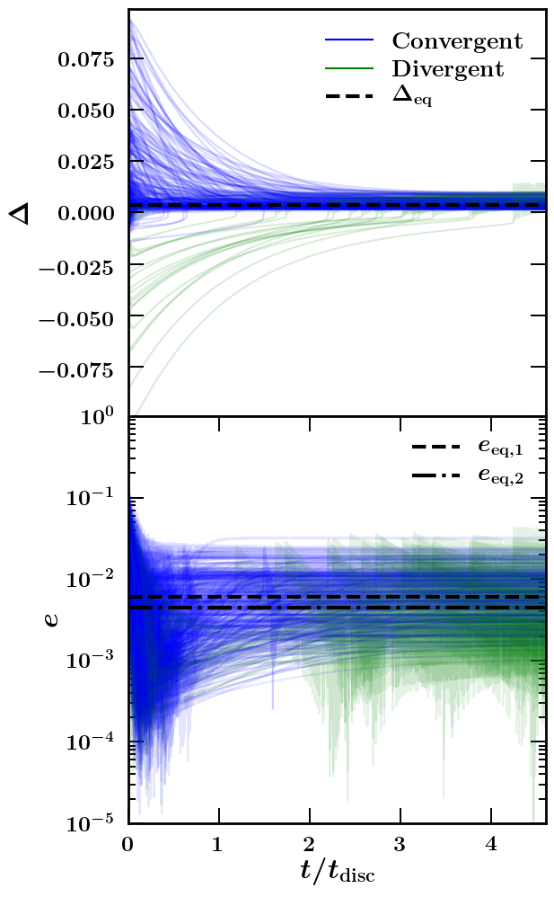
Figure 11: How systems in the peak of the $\Delta$-distribution arrived there. Only planet pairs in our $\Sigma_{0}=18$ g/cm² model with $0<\Delta_{\rm final}<0.01$ (i.e., the peak; Figure 9) are plotted here. Most systems land in the peak by migrating convergently from $\Delta_{\rm initial}>0.01$ and settling into resonant equilibria (blue curves); a few migrate divergently from $\Delta_{\rm initial}<0$ and are left in the peak when the disc disperses (green curves). Horizontal dashed line in the top panel gives the median $\Delta_{\rm eq}$ computed from equation (missing) 22 using our Monte Carlo inputs for convergent pairs only. Horizontal lines in the bottom panel give median equilibrium eccentricities computed similarly from equations (20)–(21).

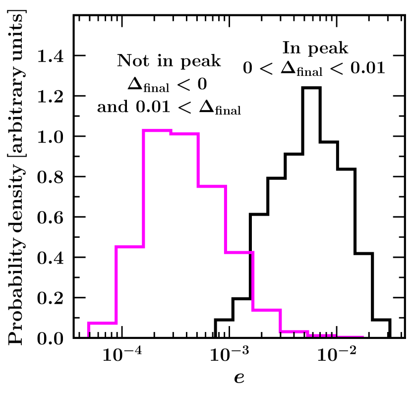
Figure 12: Final eccentricities of planets within the peak of the $\Delta$-distribution (black histogram) and outside the peak (magenta histogram), for our best-fitting $\Sigma_{0}=18$ g/cm² population synthesis model. Within the peak, eccentricities amplify from resonant migration and damp from first-order co-orbital Lindblad torques, reaching equilibrium values of $10^{-3}$–$10^{-2}$. Outside the peak, there is no resonant amplification of eccentricity, only disc damping.

Convergently migrating pairs comprising the peak equilibrate not only in $\Delta$ but also in $e$, as eccentricity pumping by resonant migration balances eccentricity damping by the disc. Figure 11 shows that eccentricities of planet pairs that convergently migrate into resonance starting from $\Delta_{\rm initial}>0.01$ equilibrate to $e_{\rm eq}\sim 10^{-3}$–$10^{-2}$ (lower panel, blue curves).

The handful of systems that find their way into the peak from $\Delta_{\rm initial}<-0.01$ exhibit similar final eccentricities, but via a different path: just after the planets cross into resonance on diverging orbits (effected either by eccentricity damping or divergent migration), their eccentricities jump to values $\gtrsim 0.01$ (Dermott et al., 1988), after which they damp back down by residual disc torques.

More generally, systems in the peak have eccentricity histories that differ from systems outside the peak, as the former have been influenced by the resonance whereas the latter have not. Figure 12 shows that, for our assumed Monte Carlo inputs (and neglecting post-formation gravitational interactions lasting Gyrs), eccentricities of non-peak systems are systematically lower than for systems in the peak.

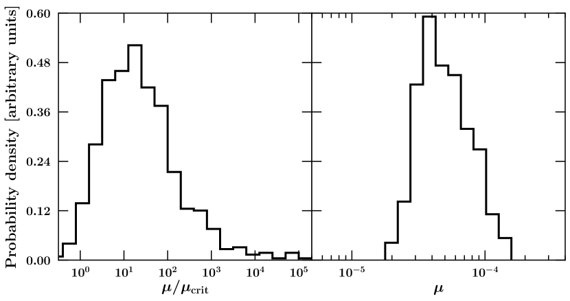
Figure 13: Distributions of $\mu/\mu_{\rm crit}$ (left panel) and $\mu$ (right panel), where $\mu=(m_{1}+m_{2})/M_{\star}$ and $\mu_{\rm crit}$ is the critical value below which the 3:2 resonance is unstable, for all convergently migrating pairs in our mock population. Our modeled sub-Neptunes, having masses between 5 and $15M_{\oplus}$, and orbiting stars between 0.5 and $2M_{\odot}$, are stable.

In our Monte Carlo calculations, convergently migrating pairs that capture into resonance stay in resonance. Escape after capture does not occur—in Figure 10, systems that convergently migrate into the shaded horizontal bar denoting $\Delta_{\rm eq}$ stay there. We checked this result by comparing our combined planet-to-star mass ratios, $\mu\equiv(m_{1}+m_{2})/M_{\star}$, to the critical value $\mu_{\rm crit}$ below which a system escapes resonance (equation 21 of Deck & Batygin 2015). The left panel of Figure 13 shows the distribution of $\mu/\mu_{\rm crit}$ for all convergently migrating pairs in our mock planet population. The distribution peaks at $\mu/\mu_{\rm crit}\sim 10$ and extends to values even larger—a consequence of comparable masses $m_{1}$ and $m_{2}$ leading to a longer relative migration timescale $t_{a}$ and thus a smaller $\mu_{\rm crit}\propto 1/t_{a}^{3/2}$ (Section 4)—demonstrating that practically all our simulated resonances are stable. Our finding contrasts with an earlier suggestion by Goldreich & Schlichting (2014, GS) that sub-Neptunes generically escape resonance (their figs. 10 and 11). The difference stems in part from our respective disc models: the GS model drops order-unity factors and fixes $t_{a}/t_{e}\equiv 3n/(2\dot{n}t_{e})=3(h/a)^{-2}/2=150$, whereas ours retains order-unity factors and $a$-dependencies (equations 15–18) to find that $t_{a}/t_{e}$ for an individual planet varies from 200 to 750 across the disc. Consequently, as $\mu_{\rm crit}\propto(t_{e}/t_{a})^{3/2}$, our values for $\mu_{\rm crit}$ are systematically lower than theirs by factors of 1.5–11. Furthermore, our combined planet-to-star mass ratios $\mu$, shown in the right panel of Figure 13, are greater than the values adopted by GS by an order of magnitude ($\mu=10^{-5}$–$10^{-4}$ vs. $10^{-6}$–$10^{-5}$). Our planet masses are modeled after radial velocity measurements (e.g., Weiss & Marcy, 2014), transit timing variations (Lithwick et al., 2012; Hadden & Lithwick, 2014, 2017), and evolutionary models for planet radius (Wu, 2019), whereas the GS values derive from planet radius measurements from 2013 and an assumed universal bulk density of 2 g/cm³.

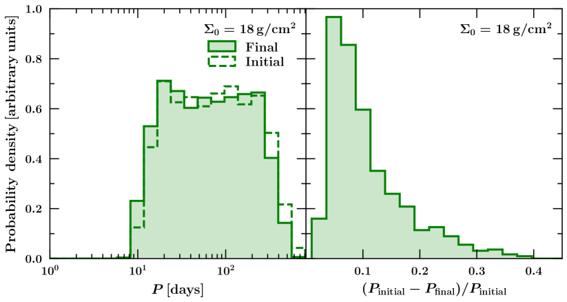
Figure 14: Final vs. initial period distributions of our mock planet population (left panel), and the fractional changes to the periods (right panel), for our best-fit $\Sigma_{0}=18$ g/cm² model. Migration is modest; the median change in orbital period is $\sim$10%.

While the relative separation $\Delta$ can increase, decrease, or equilibrate, all planets migrate inward (by construction from our adoption of Type I migration). Figure 14 compares the final distribution of individual planet periods to the initial distribution for $\Sigma_{0}=18$ g/cm², the value that gives an encouraging match to the observed $\Delta$-distribution (Figure 9). There is hardly any migration: the median change in orbital period is 10% (Figure 14, right panel). Insofar as these changes are small, sub-Neptunes can be said to have completed their mass assembly more-or-less in situ.

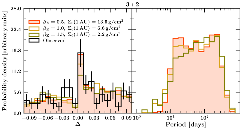
Figure 15: Attempts to reproduce the peak-trough asymmetry using alternate disc surface density profiles. Steeper profiles (larger $\beta_{\Sigma}=-d\log\Sigma/d\log a$) lead to inner planets migrating faster and fewer convergently migrating pairs, reducing the number of systems that populate the peak (left panel). With steeper profiles, more planets migrate toward the disc inner edge, producing pile-ups in the occurrence rate at short period (right panel) that are not observed (Lee & Chiang, 2017).

Finally, in Figure 15, we relax our standard assumption of a flat gas surface density profile and experiment with $\beta_{\Sigma}\equiv-d\log\Sigma/d\log a\neq 0$, with $\Sigma_{0}$ now denoting the surface density at $a=1$ au only (equation 18). As $\beta_{\Sigma}$ increases and the gas density toward the star rises, inner planets migrate faster and fewer planet pairs migrate convergently. Consequently the simulated peak in the $\Delta$-distribution weakens (left panel). Higher $\beta_{\Sigma}$ also leads to more inner planets migrating to orbital periods $P<10$ days (right panel), toward the innermost disc edge at $P=3$ days. Migrating toward the disc edge is not desirable as it leads to pile-ups in the occurrence rate at short $P$ that are not observed (Lee & Chiang, 2017). We have tried to mitigate against pile-ups by reducing $\Sigma_{0}$ as $\beta_{\Sigma}$ increases in Figure 15; however, the surface densities employed in this figure still resemble those of the disfavored migration models of Lee & Chiang (2017), which betray pile-ups that do not compare well with the observed sub-Neptune period distribution (see their figs. 4 and 5). In this regard the data appear to prefer surface densities that either stay flat or increase away from the star—these yield more convergent pairs and healthier peaks (Figure 9), while keeping migration-induced pile-ups at bay (Figure 14). Other studies have independently come to this same conclusion, as we discuss in Section 6.

6 Summary and discussion

6.1 Gas-Rich vs. Gas-Poor Discs, Migration vs. In-Situ Formation

Most pairs of sub-Neptunes and super-Earths are not in mean-motion resonance (Figure 1; Lissauer et al. 2011; Fabrycky et al. 2014). At face value, this observation suggests that disc-driven migration plays only a limited role in the formation of such planets, as wholesale changes to orbital periods would be expected to capture a large fraction of bodies into resonance. Goldreich & Schlichting (2014) warned against this conclusion, pointing out that sufficiently low-mass planets escape from resonance when their eccentricities are damped by interactions with their natal discs. While our calculations confirm the existence of a planetary system mass below which resonances are overstable, we find that most sub-Neptune pairs sit above this threshold, and their resonances are therefore stable against eccentricity damping. Current inferences of sub-Neptune masses from radial velocity measurements (e.g., Weiss & Marcy, 2014), transit timing variations (Lithwick et al., 2012; Hadden & Lithwick, 2014, 2017), and theoretical radius-mass relations incorporating photoevaporative mass loss (Wu, 2019) indicate planet-to-star mass ratios at least a factor of $\sim$10 higher than the values used by Goldreich & Schlichting (2014); compare our Figure 13 to their fig. 10.

While most planet pairs are not in resonance, some are. There are excess numbers of systems just wide of resonance, with $0<\Delta\lesssim 0.02$, where $\Delta$ is the fractional deviation of a pair’s period ratio away from 3/2 or 2/1 (equation 1). Accompanying these excesses are deficits in the planet population just short of resonance, with $-0.02\lesssim\Delta<0$. We have sought to reproduce this “peak-trough” feature in the $\Delta$-histogram by modeling the dynamical evolution of planets within their natal discs. In our model, the peak mostly comprises pairs of planets each of which convergently migrated from $\Delta_{\rm initial}>0.01$, captured into resonance, and attained an equilibrium wherein migration-induced, resonant amplification of eccentricities balances disc damping of eccentricities. This eccentricity equilibrium corresponds, in resonance, to an equilibrium in relative semi-major axes, i.e., an equilibrium in $\Delta$ (e.g., Terquem & Papaloizou, 2019). For our model parameters, $\Delta_{\rm eq}=0.001$–0.01, which matches well the position of the peak for the 3:2 resonance, at least for periods longer than $\sim$5 days (more on the 2:1 resonance in Section 6.2 below). The trough corresponds to systems that begin at $-0.01<\Delta_{\rm initial}<0$ and are transported into resonance at $\Delta>0$ by disc eccentricity damping. The parameters responsible for this quantitative agreement include disc aspect ratios of $h/a\simeq 0.02$–0.04, appropriate for the $a=0.1$–1 au orbital distances of Kepler planets, and planet-pair-to-star mass ratios of $\mu\sim 10^{-5}$–$10^{-4}$.

The more massive the disc and the longer it persists, the farther away a pair can be from resonance (i.e., the larger $\Delta_{\rm initial}$ can be) and still be brought into resonant contact by migration—more migration brings more systems into the peak. The observed peak and trough for the 3:2 resonance are approximately reproduced for a disc e-folding time of $t_{\rm disc}=10^{5}$ yr and a gas surface density of $\Sigma_{0}\sim 20$ g/cm² at orbital distances $a=0.1$–1 au (Figure 9). An equivalent fit is obtained for $t_{\rm disc}=10^{6}$ yr and $\Sigma_{0}\sim 2$ g/cm².

Gas surface density profiles that are flat if not actually rising with distance from the host star are preferred as they lead to a greater proportion of planet pairs that migrate convergently and efficiently populate the peak. Gas profiles that fall steeply away from the star (like that of the minimum-mass nebula, $\Sigma\propto a^{-3/2}$) are disfavored because they lead to a smaller fraction of convergent pairs; faster migration rates, i.e., higher overall surface densities, are then needed to reproduce the peak, but these lead to pile-ups of sub-Neptunes near the disc inner edge that violate observed occurrence rate profiles (Lee & Chiang, 2017).

Since we do not follow the growth of planet masses, but merely mock up their present-day values, our model gas surface densities should be interpreted as characterizing the disc around the time planets complete their assembly, during or just after their last mass doubling. The gas densities we have inferred from fitting the peak-trough feature are low: 2–20 g/cm² is 3–5 orders of magnitude lower than the gas content of a minimum-mass, solar composition nebula at the relevant orbital distances. Our preferred model disc appears incompatible with gas-rich scenarios (e.g., pebble accretion) for super-Earth and sub-Neptune formation. Our results point instead to gas-poor formation scenarios, in particular giant impacts (e.g., Dawson et al., 2015; Lee, 2019; MacDonald et al., 2020). Our fitted nebular densities are quantitatively consistent with the formation of super-Earth/sub-Neptune cores by giant impacts; gas densities are sufficiently low, and by extension disc eccentricity damping is sufficiently weak, that proto-cores, each a few Earth masses and spaced several Hill radii apart, can gravitationally stir one another onto crossing orbits and merge into full-fledged super-Earths (see, e.g., the $k=7$ curve in fig. 5 of Lee & Chiang 2016). Although we need planets to migrate to produce the peak, they should not migrate by much, as otherwise the magnitude of the peak would be overestimated: in our preferred model, the median change in the orbital period of an individual planet is only 10% (Figure 14). Accordingly, we would describe the endgame of sub-Neptune formation as occurring largely in situ. This same conclusion is reached by Terquem & Papaloizou (2019). Furthermore, MacDonald & Dawson (2018) show that the handful of multi-planet resonant chains like Kepler-223 (Mills et al., 2016) and Trappist-1 (Gillon et al., 2017) do not necessarily implicate wholesale migration, but can also be established by more modest “short-scale” migration, as advocated here.

Encouragingly, our preferred low-mass disc with a flat-to-rising surface density profile resembles disc models computed by Suzuki et al. (2016) using strongly magnetized winds to drive accretion (see their fig. 1, the red or green curves). Ogihara et al. (2018) have shown that sub-Neptunes within such discs undergo their last mass doubling/giant impact around $10^{6}$ yr (their fig. 3c), at which time the surface density at 0.1–1 au is about $20$ g/cm² (their fig. 1a). Their calculated final period distribution of sub-Neptunes matches that observed (their fig. 14), with no pile-ups from excessive migration. The largely in-situ formation history described by these authors agrees with ours.

6.2 Tides and the 2:1 and 3:2 Resonances

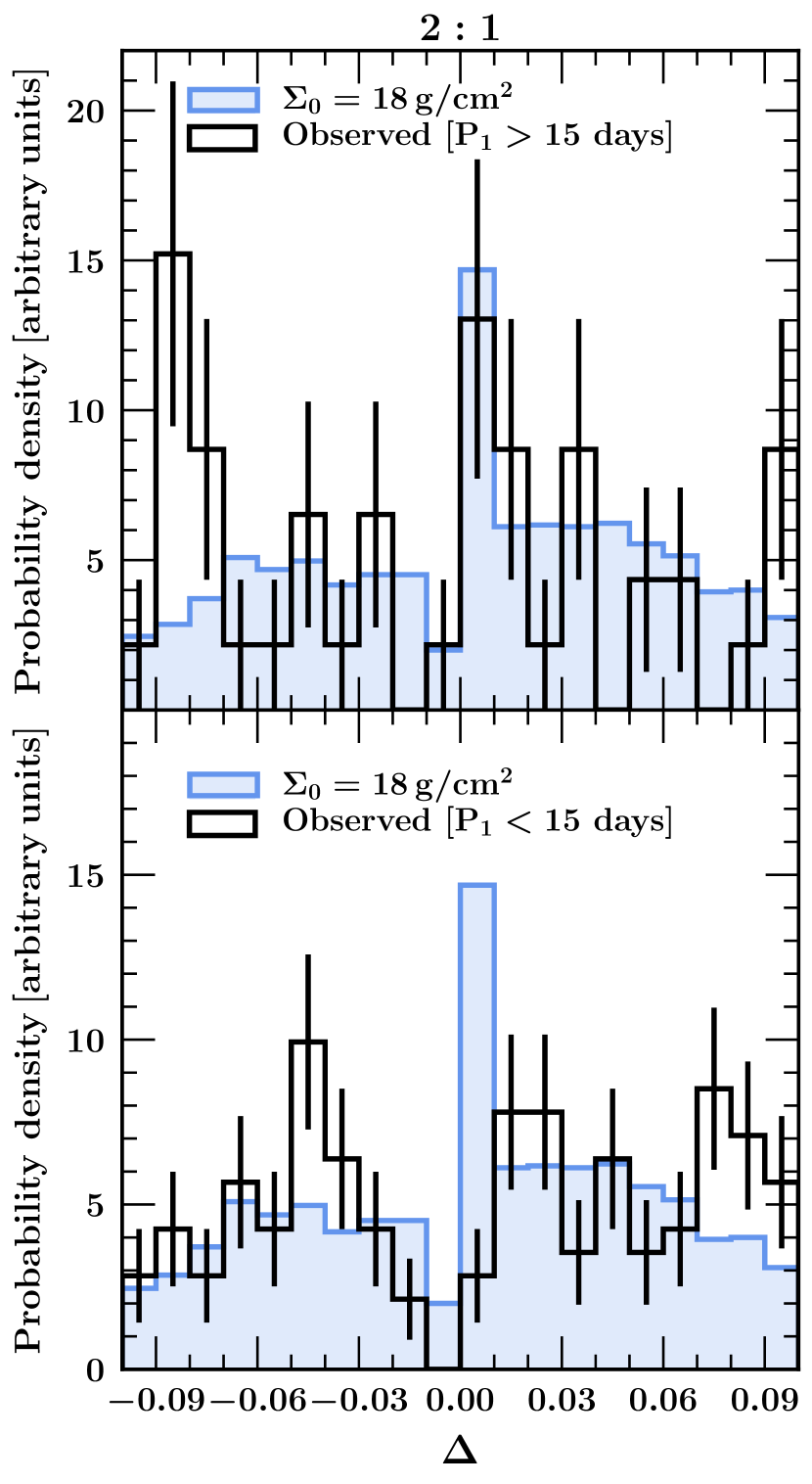
Figure 16: The $\Delta$-distribution for the 2:1 resonance, observed (black) and modeled (blue). The observational data are split according to the period of the inner planet $P_{1}$. At $P_{1}>15$ days (upper panel), systems are presumably least impacted by stellar tidal interactions, and the peak-trough asymmetry can be reproduced by our disc-only, no-tide model. Disc parameters are the same as those fitted for the 3:2 ($\Sigma_{0}=18$ g/cm², $\beta_{\Sigma}=0$, $t_{\rm disc}=10^{5}$ yr), while the resonance parameters are appropriate for the 2:1 ($\alpha=(1/2)^{2/3}$, $f_{1}=-1.190$, and $f_{2}=1.688$). At $P_{1}<15$ days (lower panel), the observed peak shifts to larger $\Delta$ than is predicted by our model, and the trough is wider, presumably reflecting post-disc tidal dissipation.

We have focussed so far on using planet-disc interactions, and not stellar tidal effects, to reproduce the $\Delta$-distribution near the 3:2 resonance. The 3:2 data exhibit the strongest peak-trough asymmetry. These data also appear, as judged by their relative insensitivity to orbital period (Figures 2 and 3), the least impacted by stellar tides. A non-trivial test of our model is to see whether it can simultaneously reproduce the 2:1 $\Delta$-distribution, at least at the longest periods where potential complications from tides are minimal. Our model appears to pass this test: Figure 16 demonstrates that our best-fit disc model for the 3:2 reproduces the 2:1 reasonably well at inner planet periods $P_{1}>15$ days (top panel). We emphasize that we have not tuned any of our disc parameters to fit for the 2:1; we have merely taken the same background disc that we fitted for the 3:2 ($\Sigma_{0}\sim 20$ g/cm², $t_{\rm disc}=10^{5}$ yr) and asked whether it reproduces the 2:1. It does.

We have looked to the parent disc to change planet semi-major axes and eccentricities. While Millholland & Laughlin (2019, ML) also looked to the disc to drive semi-major axis changes, they appealed to tidal friction, specifically the heat generated by obliquity tides raised on planets by their host stars, for an additional energy sink to drive resonant repulsion. All of our results indicate that, at long enough periods, the disc suffices as a source of dissipation. Eccentricity damping by the disc is neglected by ML but is part and parcel of the disc-planet torque. In concert with disc-driven migration, disc eccentricity damping creates the peak-trough features at $\Delta=\pm\,0.01$ seen at large periods for both the 3:2 and 2:1 resonances, with no need for extra damping.

The picture complicates, however, at the shortest periods. At $P_{1}<15$ days (bottom panel in Figure 16), the disc-only, no-tide model is not a good fit to the 2:1: the observed 2:1 peak is lower in amplitude and displaced to larger $\Delta$, and the observed 2:1 trough is wider. Future work needs to resolve these discrepancies. Planets in the 2:1 are situated farther apart than in the 3:2, making the 2:1 more prone to disruption (say by other planets in the system), and possibly less prone to convergent migration (see the end of this section for why); both effects would reduce the height of the 2:1 peak. The larger separation also renders 2:1 systems less sensitive to their mutual resonant forcing and more sensitive to stellar tides. The shift of the location of the peak toward larger $\Delta$ with decreasing period (Figures 2 and 3) seems best explained by tides. In this context the ML scenario specifically calls out the 2:1 over the 3:2: ML argued that the parameter space for spin-orbit resonance capture and obliquity-driven tidal dissipation is larger for the 2:1 than for the 3:2, and Millholland (2019) uncovered observational evidence for greater tidal heating of planets in the 2:1 than the 3:2. The emerging qualitative picture is that planet-disc interactions establish, over Myrs, a baseline peak-trough asymmetry at all periods (this paper), while tides take this baseline at the shortest periods and modify it over Gyrs (ML). Asynchronous tides raised on host stars by planets might also have a role to play—these cause planets to migrate inward and divergently, further shifting the peak to larger $\Delta$ (Lee & Chiang 2017, their fig. 10).

Whereas our model requires only small, $\sim$10% changes to orbital periods that are consistent with the lack of observed planet pile-ups at short period (Ogihara et al., 2018; Lee & Chiang, 2017; Dressing & Charbonneau, 2015; Fressin et al., 2013), it is not clear whether disc-driven migration in the ML scenario is similarly compatible. In the example evolution shown in fig. 3 of ML, planet orbital periods change by $\sim$70–80%: first to cross a spin-orbit resonance, then to capture into 3:2 resonance, and finally to capture into spin-orbit resonance and generate a large permanent obliquity. Adjusting initial conditions and parameters may reduce the degree of migration needed in the ML scenario. What should also help is an accounting for how planetary precession rates change as the disc dissipates (an effect omitted by ML and by us); explicitly time-varying precession can lead to spin-orbit resonance crossings with less need for semi-major axis changes (see, e.g., Ward 1981).

There are other open questions. How does the $\Delta$-distribution change post-disc, over Gyrs of gravitational interactions between planets? Diffusion of systems in $\Delta$ would erode the peak-trough asymmetry, with the lower survival probability of systems at $\Delta<0$ compensating in part (Pu & Wu, 2015). The free eccentricities (resonant libration amplitudes) of our modeled planets in the peak are damped to zero by the disc; how do we raise them to reproduce resonant systems with observed free eccentricities of order 1% (Lithwick et al., 2012; Hadden & Lithwick, 2014, 2017)? Here also post-formation interplanetary interactions should be investigated. Finally, most planet pairs in the peak arrived there in our model by convergent migration. Whether migration is convergent or divergent depends on how the disc is structured (how its aspect ratio and surface density change with radius), and the mass ratio $m_{2}/m_{1}$ of the outer planet to the inner. Mass measurements by Hadden & Lithwick (2017) using transit timing variations indicate that $m_{2}/m_{1}>1$ about as often as $m_{2}/m_{1}<1$ for planet pairs near resonance peaks. What do these mass ratio statistics imply about disc structure, assuming these pairs migrated convergently? Pairs with $m_{2}/m_{1}<1$ can still migrate convergently if the surface density rises with increasing distance from the host star, as it does in the wind-driven disc models of Suzuki et al. (2016). Planetary orbits also converge regardless of $m_{2}/m_{1}$ if a common gap is opened between them (Masset & Snellgrove, 2001; Fung & Chiang, 2017). The closer the planets, the more easily planetary Lindblad torques clear a common gap; thus we would expect more convergent pairs capturing into the 3:2 than into the (more separated) 2:1. Indeed the peak for the 3:2 is stronger than for the 2:1.

Appendix A Host Star Spectral Type

In Figure 17 we plot the distribution of period ratios of pairs of sub-Neptunes, distinguishing between those with FGK host stars and those with M host stars. Compared to Figure 1, the statistics in Figure 17 are poorer, not only because we are splitting the data but because we had to discard the many entries in the NASA Exoplanet Archive that do not specify host star spectral type (Figure 1 plots all systems regardless of whether they have a spectral type listed or not). As far as we can tell from Figure 17, the peak-trough asymmetries near the 3:2 and 2:1 resonances are common to sub-Neptunes around both FGK and M stars.

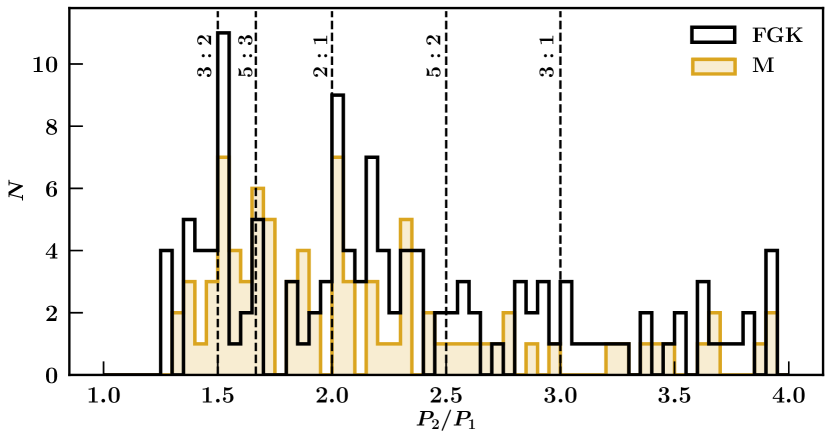
Figure 17: Same as Figure 1 but now differentiating between FGK host stars and M stars. The period ratio asymmetries near first-order resonances are evident for all spectral types.

References

- Agol et al. (2005) Agol E., Steffen J., Sari R., Clarkson W., 2005, MNRAS, 359, 567
- Alexander et al. (2014) Alexander R., Pascucci I., Andrews S., Armitage P., Cieza L., 2014, in Beuther H., Klessen R. S., Dullemond C. P., Henning T., eds, Protostars and Planets VI. p. 475 (arXiv:1311.1819), doi:10.2458/azu_uapress_9780816531240-ch021
- Artymowicz (1993) Artymowicz P., 1993, ApJ, 419, 155
- Batygin & Morbidelli (2013) Batygin K., Morbidelli A., 2013, AJ, 145, 1
- Bitsch et al. (2019) Bitsch B., Izidoro A., Johansen A., Raymond S. N., Morbidelli A., Lambrechts M., Jacobson S. A., 2019, A&A, 623, A88
- Chiang & Goldreich (1997) Chiang E. I., Goldreich P., 1997, ApJ, 490, 368
- Chiang & Laughlin (2013) Chiang E., Laughlin G., 2013, MNRAS, 431, 3444
- Cresswell et al. (2007) Cresswell P., Dirksen G., Kley W., Nelson R. P., 2007, A&A, 473, 329
- Dawson et al. (2015) Dawson R. I., Chiang E., Lee E. J., 2015, MNRAS, 453, 1471
- Deck & Batygin (2015) Deck K. M., Batygin K., 2015, ApJ, 810, 119
- Delisle & Laskar (2014) Delisle J. B., Laskar J., 2014, A&A, 570, L7
- Dermott et al. (1988) Dermott S. F., Malhotra R., Murray C. D., 1988, Icarus, 76, 295
- Dressing & Charbonneau (2015) Dressing C. D., Charbonneau D., 2015, ApJ, 807, 45
- Duffell & Chiang (2015) Duffell P. C., Chiang E., 2015, ApJ, 812, 94
- Fabrycky et al. (2014) Fabrycky D. C., et al., 2014, ApJ, 790, 146
- Fressin et al. (2013) Fressin F., et al., 2013, ApJ, 766, 81
- Fung & Chiang (2017) Fung J., Chiang E., 2017, ApJ, 839, 100
- Gillon et al. (2017) Gillon M., et al., 2017, Nature, 542, 456
- Goldreich & Sari (2003) Goldreich P., Sari R., 2003, ApJ, 585, 1024
- Goldreich & Schlichting (2014) Goldreich P., Schlichting H. E., 2014, AJ, 147, 32
- Goldreich & Tremaine (1980) Goldreich P., Tremaine S., 1980, ApJ, 241, 425
- Hadden & Lithwick (2014) Hadden S., Lithwick Y., 2014, ApJ, 787, 80
- Hadden & Lithwick (2017) Hadden S., Lithwick Y., 2017, AJ, 154, 5
- Hunter (2007) Hunter J. D., 2007, Computing In Science & Engineering, 9, 90
- Izidoro et al. (2017) Izidoro A., Ogihara M., Raymond S. N., Morbidelli A., Pierens A., Bitsch B., Cossou C., Hersant F., 2017, MNRAS, 470, 1750
- Izidoro et al. (2019) Izidoro A., Bitsch B., Raymond S. N., Johansen A., Morbidelli A., Lambrechts M., Jacobson S. A., 2019, arXiv e-prints, p. arXiv:1902.08772
- Kley & Nelson (2012) Kley W., Nelson R. P., 2012, ARA&A, 50, 211
- Kominami & Ida (2002) Kominami J., Ida S., 2002, Icarus, 157, 43
- Lambrechts et al. (2019) Lambrechts M., Morbidelli A., Jacobson S. A., Johansen A., Bitsch B., Izidoro A., Raymond S. N., 2019, A&A, 627, A83
- Lee (2019) Lee E. J., 2019, ApJ, 878, 36
- Lee & Chiang (2016) Lee E. J., Chiang E., 2016, ApJ, 817, 90
- Lee & Chiang (2017) Lee E. J., Chiang E., 2017, ApJ, 842, 40
- Lee & Peale (2002) Lee M. H., Peale S. J., 2002, ApJ, 567, 596
- Lee et al. (2013) Lee M. H., Fabrycky D., Lin D. N. C., 2013, ApJ, 774, 52
- Lee et al. (2018) Lee E. J., Chiang E., Ferguson J. W., 2018, MNRAS, 476, 2199
- Lissauer et al. (2011) Lissauer J. J., et al., 2011, ApJS, 197, 8
- Lithwick & Wu (2012) Lithwick Y., Wu Y., 2012, ApJ, 756, L11
- Lithwick et al. (2012) Lithwick Y., Xie J., Wu Y., 2012, ApJ, 761, 122
- MacDonald & Dawson (2018) MacDonald M. G., Dawson R. I., 2018, AJ, 156, 228
- MacDonald et al. (2020) MacDonald M. G., Dawson R. I., Morrison S. J., Lee E. J., Khandelwal A., 2020, ApJ, 891, 20
- Masset & Snellgrove (2001) Masset F., Snellgrove M., 2001, MNRAS, 320, L55
- Meyer & Wisdom (2008) Meyer J., Wisdom J., 2008, Icarus, 193, 213
- Millholland (2019) Millholland S., 2019, arXiv e-prints, p. arXiv:1910.06794
- Millholland & Laughlin (2019) Millholland S., Laughlin G., 2019, Nature Astronomy, 3, 424
- Mills et al. (2016) Mills S. M., Fabrycky D. C., Migaszewski C., Ford E. B., Petigura E., Isaacson H., 2016, Nature, 533, 509
- Murray & Dermott (1999) Murray C. D., Dermott S. F., 1999, Solar system dynamics
- Ogihara et al. (2018) Ogihara M., Kokubo E., Suzuki T. K., Morbidelli A., 2018, A&A, 615, A63
- Papaloizou & Larwood (2000) Papaloizou J. C. B., Larwood J. D., 2000, MNRAS, 315, 823
- Papaloizou & Terquem (2010) Papaloizou J. C. B., Terquem C., 2010, MNRAS, 405, 573
- Peale (1986) Peale S. J., 1986, Orbital resonances, unusual configurations and exotic rotation states among planetary satellites. pp 159–223
- Petigura et al. (2018) Petigura E. A., et al., 2018, AJ, 155, 89
- Pu & Wu (2015) Pu B., Wu Y., 2015, ApJ, 807, 44
- Rein (2012) Rein H., 2012, MNRAS, 427, L21
- Rosenthal & Murray-Clay (2019) Rosenthal M. M., Murray-Clay R. A., 2019, arXiv e-prints, p. arXiv:1908.06991
- Sandford et al. (2019) Sandford E., Kipping D., Collins M., 2019, MNRAS, 489, 3162
- Silburt & Rein (2015) Silburt A., Rein H., 2015, MNRAS, 453, 4089
- Suzuki et al. (2016) Suzuki T. K., Ogihara M., Morbidelli A. r., Crida A., Guillot T., 2016, A&A, 596, A74
- Terquem & Papaloizou (2019) Terquem C., Papaloizou J. C. B., 2019, MNRAS, 482, 530
- Ward (1981) Ward W. R., 1981, Icarus, 47, 234
- Ward (1997) Ward W. R., 1997, ApJ, 482, L211
- Weiss & Marcy (2014) Weiss L. M., Marcy G. W., 2014, ApJ, 783, L6
- Wu (2019) Wu Y., 2019, ApJ, 874, 91
- Xu & Lai (2017) Xu W., Lai D., 2017, MNRAS, 468, 3223
- Xu et al. (2018) Xu W., Lai D., Morbidelli A., 2018, MNRAS, 481, 1538
- Zhu et al. (2018) Zhu W., Petrovich C., Wu Y., Dong S., Xie J., 2018, ApJ, 860, 101