Improving sampling and calibration of GRBs as distance indicators

Abstract

We present a sample of 74 Gamma-Ray Bursts (GRBs) from the Fermi-GBM catalogue for which we compute the distance moduli and use them to constrain effective dark energy models. To overcome the circularity problem affecting GRBs as distance indicators, we calibrate the Amati relation of our sample with a cosmology-independent technique. Specifically, we use the latest observational Hubble parameter data, including associated systematics, to approximate the cosmic expansion through a Bezier parametric curve. We subsequently obtain the distance moduli of the GRBs and include the data in a suite of recent cosmological observations of the expansion history (Planck Compressed 2018, 2012 BOSS release of BAO data and Pantheon SNIa), to compute Bayesian posterior constraints for the standard cosmological model $\Lambda$CDM, as well as $\omega$CDM, and the CPL parametrization. Throughout the analysis we strive to keep under control the error propagation and limit our GRBs sample to avoid observational bias. As a result, we find no evidence in favour of the alternatives to $\Lambda$CDM model. The latter agrees very well with our calibrated sample of GRBs and presently available luminosity distance probes.

1 Introduction

In the endeavour to characterise the cosmological expansion, standard candles are a keystone for precise distance determinations. In practice, however, the demand for high precision in many of the distance indicators exposes several sources of bias that prevent astrophysical objects from reaching the status of standard candles. The luminosity of Supernovae of Type Ia (SNe Ia), for example, is thought to be subject to its environment (Kang et al., 2020) and such dependence could only be accounted for through precise observations. See however, the recent analysis of Rose et al. (2020) which reports no evidence for such dependence.

In this sense, any contribution from alternative distance indicators, preferably covering a wide range of redshifts, is key to improve cosmological distance determinations, and ultimately, characterise the Dark Energy component.

An attractive prospect is the distance modulus of Gamma Ray Bursts (GRBs). For pioneer works see e.g., Ghirlanda et al. (2004a); Liang & Zhang (2005); Firmani et al. (2005); Schaefer (2007). Despite the well known dispersion in the luminosity correlations and other sources of uncertainty, GRBs remain good candidates for distance indicators.

GRBs account for the most powerful explosions in the Universe; they are bright enough to be detected up to high redshifts. Therefore, they are often proposed as complementary tools to SNe Ia observations to probe the expansion history of the Universe. The prompt emission of GRBs lies mostly in the range from $0.001$ to a few MeV, and lasting from $0.01$ to $1000$ seconds. This property classifies naturally the set of GRBs into two categories, those with $T{90}>2$ seconds are classified as long and are associated to the collapse of certain types of massive stars. On the other hand, the short kind is associated to the merger of compact objects (Meszaros, 2006). Despite several efforts to model the explosion mechanism of the GRBs (e.g., Mendoza et al., 2009; Rivera-Paleo & Guzman, 2016; Dainotti et al., 2018; Stratta et al., 2018), there is no single satisfactory explanation and their nature is still not fully understood. In consequence, the distance calibration of GRBs presents more difficulties than that of SNe Ia.

So far, several methods have been proposed to calibrate GRBs (Liang & Zhang, 2005; Firmani et al., 2005; Schaefer, 2007; Liang et al., 2008; Liang & Zhang, 2008; Wei & Zhang, 2009; Kodama et al., 2008; Wang, 2008; Liu & Wei, 2015). Most calibrating methods rely on empirical luminosity correlations found in long GRBs. Among the known correlations are those between spectrum lag and isotropic peak luminosity ($\tau_{\rm lag}-L$ relation of Norris et al. (2000)), the correlation between time variability and isotropic peak luminosity ($V-L$ relation proposed by Fenimore & Ramirez-Ruiz (2000)), a tight correlation between the peak energy of $\nu F_{\nu}$ spectrum and isotropic equivalent energy ($E_{\rm p}-E_{\mathrm{iso}}$ relation of Amati et al. (2002)), a correlation between the peak energy and the collimation-corrected energy ($E_{\rm p}-E_{\gamma}$ relation proposed by Ghirlanda et al. (2004b)), the correlation between peak energy and isotropic peak luminosity ($E_{\rm p}-L$ relation of Yonetoku et al. (2004)), the correlation between the isotropic peak luminosity, the peak energy and the high signal time-scale, ($L_{\rm iso}-E_{\rm p}-T_{0.45}$ relation by Firmani et al. (2006a)) and the correlation between minimum rise time of light curve and isotropic peak luminosity ($\tau_{\rm RT}-L$ relation of Schaefer (2007)). Recently, some other correlations have been reported in the literature (Dainotti et al., 2008; Liang et al., 2010; Ghirlanda et al., 2011; Xu & Huang, 2012; Lü et al., 2012; Yi et al., 2015; Liang et al., 2015). For a review and more details about them, see for instance Zhang (2018).

In many of the above, the luminosity of GRBs appears correlated with the temporal and spectral properties. While such correlations are not fully understood from first principles, their existence naturally leads to the consideration that GRBs could be used as distance indicators, offering a route to probe the expansion history of the Universe up to $z\gtrsim 9$. Datasets of GRBs distance moduli are often used (either alone or in combination with other observational data such as SNe Ia), to constrain cosmological parameters (e.g. Ghirlanda et al., 2004a; Firmani et al., 2005; Liang & Zhang, 2005; Schaefer, 2007; Liang et al., 2008; Liang & Zhang, 2008; Wei & Zhang, 2009; Wei, 2010; Montiel & Breton, 2011; Velten et al., 2013; Bretón & Montiel, 2013; Amati & Della Valle, 2013; Wang et al., 2015). It is important to note that in the calibration of empirical correlations, two caveats stand out that prevent the improvement of GRBs distance moduli as distance indicators. First is a number of sources of uncertainty in the determination of luminosity parameters. It is known that combining databases from different telescopes may introduce an unknown selection bias due to the different thresholds and spectroscopic sensitivity (Butler et al., 2007; Nava et al., 2008). Additionally, mixing methods for the redshift determination (photometric vs. spectral) also represents a source for uncertainty (Coward, 2009).

The purpose of the present work is to present a new and independent dataset of GRBs addressing the above issues and show their usefulness as distance indicators. To overcome the aforementioned shortcomings, we consider data exclusively from a single catalogue (the Fermi-GBM catalogue), which prevents selection biases and other instrument-associated systematics. Moreover, to avoid extra bias, instead of using the complete set of long GRBs with available redshift, we select only those with redshift determined through spectroscopic methods.

An important drawback of the usual GRBs calibration as distance indicators is an inherent circularity problem, since the determination of energy flux typically assumes an underlying cosmological model. Several works have attempted to tackle these circularity problems by adopting model-independent methods to estimate parameters in the calibration (see for instance Liang & Zhang (2006); Li et al. (2008); Firmani et al. (2005); Li et al. (2008); Liang et al. (2008); Kodama et al. (2008); Liang & Zhang (2008); Wei & Zhang (2009); Montiel & Breton (2011); Velten et al. (2013); Bretón & Montiel (2013)). Here we adopt the strategy presented by Amati et al. (2019) to overcome this problem.

This paper presents a sample of 74 Fermi-GRBs, carefully selected to avoid speculation, and consequently large uncertainty, in the determination of luminosity parameters. After listing their spectral properties, we calibrate the set in a model-independent way by employing the Amati relation (Amati & Della Valle, 2013; Amati et al., 2008) which relates the rest frame peak energy of the spectra $E_{\rm p}$ to the isotropic energy emitted $E_{\mathrm{iso}}$. The calibration is performed following the recent work of Amati et al. (2019) where a compilation of 31 measurements of the Hubble parameter was used to fit a Bezier parametric curve in order to obtain the Hubble’s rate at arbitrary redshifts without assuming an a priori cosmological model. In that paper, the values for the $E_{\mathrm{iso}}$ was determined for 193 GRBs taken from Demianski et al. (2017a) and references therein. In the present work, in contrast, our sample stems from a single catalogue and in the calibration process we take into account the impact of systematic uncertainties of the Hubble parameter measurements (coming from the stellar population synthesis model, and stellar metallicity among others); an aspect overlooked in previous works. Moreover, we take special care in propagating the uncertainties of the best-fit parameters for the Bezier curve as well as for the Amati relation.

The usefulness of our dataset is demonstrated by comparing our results with previous samples through a Bayesian parameter estimation, performed for three popular effective Dark Energy models. Namely, the $\Lambda$ cold dark matter ($\Lambda$CDM), the $\omega$ cold dark matter ($\omega$CDM), and the Chevalier-Polarski-Linder (CPL) models. The parameter estimation is carried employing the GRB data and the latest compilation of Supernovae Ia data (SNe Ia) (Scolnic et al., 2018), Baryon Acoustic Oscillations (BAO) (Alam et al., 2017; Beutler et al., 2011; Ross et al., 2015), and Cosmic Microwave Background (CMB) data (Chen et al., 2019).

The paper is organized as follows. In Sec. 2 we present in detail our Fermi/GBM GRBs sample; in Sec. 3 we calibrate the observables of our sample and subsequently the Amati relation. In Sec. 4 we present the three dark energy (DE) models studied in this work. In Sec. 5 we present the datasets included in our suite of observations to fit parameters of DE models. We discuss our results in Sec. 6 and draw conclusions in Sec. 7.

2 Gamma-Ray Bursts observations

The GRBs spectrum is mainly, but not exclusively, described in terms of an empirical spectral function, the Band function (Band et al., 1993), which is explicitly

$$f(E)=\begin{cases}N_{0}\left(\dfrac{E}{100\text{keV}}\right)^{\alpha}\exp\left(-\dfrac{E}{E_{0}}\right)&E\leq E_{b}\\ \\ N_{0}\left(\dfrac{E_{b}}{\text{100keV}}\right)^{(\alpha-\beta)}\exp(\beta-\alpha)\left(\dfrac{E}{100\text{keV}}\right)^{\beta}&E>E_{b}\end{cases}$$ (1)

with $E_{b}=(\alpha-\beta)E_{0}$. This spectrum peaks at (E_p,obs), which is related to the spectral parameters as $E_{\rm p,obs}=E_{0}(2+\alpha)$.

Due to the intense radiation emitted in GRBs, it is possible to detect such explosions at high redshift $z$ (Salvaterra et al., 2009). The precise determination of $z$ is crucial to infer the distance to the object (luminosity distance), which is necessary to determine the radiated energy ($E_{\rm iso}$) in gamma rays. The redshift can be computed analysing spectral emission or absorption lines of the afterglow spectrum, or by its photometric analysis at lower energy bands (from X-rays to radio), from observations generally performed by auxiliary telescopes .

2.1 The sample

While the SWIFT satellite has provided the largest number of GRBs with redshift to the existing catalogues, the BAT instrument of this satellite is limited to energies up to $150$ keV (Gehrels et al., 2004). This value lies below the average $E_{\rm p,obs}$ of GRBs (Kaneko et al., 2006), which prevents the determination of most of the spectral parameters in the Band function or even the cut-off power-law. Consequently, it is impossible to obtain directly the flux and luminosity for many of the GRBs observed by the BAT-SWIFT satellite.

On the other hand, Fermi features two instruments GBM and LAT sensible to energy bands of 8 keV to 40 MeV (Meegan et al., 2009), and 100 MeV to 300 GeV (Atwood et al., 2009), respectively.

After SWIFT-BAT, FERMI-GMB is the instrument with the largest count of long GRBs with redshift, with the advantage that GMB allows for the determination of all the spectral parameters in the Band function. This is why we have compiled and reduced a sample of long GRBs with known redshift exclusively from the FERMI-GBM catalogue (recall that the short GRBs do not satisfy the same Amati relation as that of the long GRBs and they are also discarded from our sample).

Including long GRBs from other telescopes aside from FERMI-GBM pertains observational biases caused by the different sensitivities in the range of energy intervals and energy fluxes for each instrument (Ghirlanda et al., 2008; Nava et al., 2008; Ghirlanda et al., 2012). Such biases bring uncertainties to the determination of the fluence, and we avoid them by limiting the size of our sample, in contrast with other recent compilations (see e.g. Amati et al., 2019; Demianski et al., 2019).

For our compilation, FERMI spectral data were taken from the FERMI-GBM catalogue including observations from August 2008 to March 2019 (107 long GRBs) compiled by von Kienlin et al. (2020); Gruber et al. (2014); von Kienlin et al. (2014). The redshifts were retrieved from the BAT-SWIFT database available at https://swift.gsfc.nasa.gov/archive/grb_table.html/ and the webpage of J. Greiner http://www.mpe.mpg.de/~jcg/grbgen.html. Noting that some of the GRBs listed in the FERMI-GBM catalogue present no value for the spectral parameters, we reduced the raw data, employing the Gamma Ray Spectral Fitting Package (RMFIT V4.3.2). In particular, we did this for the cases of GRB120712571, GRB180728728, GRB181020792, GRB190114873, GRB190324947.

Since the determination of redshift from photometry is subject to the learning-curve effect, that is, there is a drift in the mean redshift over time as a consequence of different instruments contributing to redshift acquisition (see e.g. Coward (2009)), we avoid further bias and discard 8 GRBs with redshift set through such method (Nava et al., 2012a). Thus, we limit our sample to those GRBs with redshift determined through spectroscopic methods either from the afterglow or from the host galaxy. In addition, we discard 7 events (GRB080905705, GRB091020900, GRB101219686, GRB120907017, GRB121211574, GRB130612141 and GRB180205184), that present a low signal-to-noise or an incomplete light curve which lead to highly uncertain spectral parameters.

In the same spirit, we also discard 18 GRBs which present significant uncertainties in the spectral parameters, namely $E_{\rm p}$ and $F_{\rm bolo}$, because of their poor contribution to the fitting procedure.

In sum, after selecting objects meeting the above criteria, from the initial sample of 107 GRBs we finally present in Table 1 a sample of 74 GRBs covering the redshift range $0.117\leq z\leq 5.283$, together with their spectral parameters and their associated errors.

In the following section we describe the method to derive the distance moduli for these objects.

GRB	z	t90	N0	$\sigma_{\rm N_{0}}$	$E_{\rm p,obs}$	$\sigma_{E_{\rm p,obs}}$	$\alpha$	$\sigma_{\alpha_{0}}$	$\beta$	$\sigma_{\beta}$	Fbolo	$\sigma_{F_{\rm bolo}}$
		[s]	[ph/cm2s keV]	[ph/cm2s keV]	[keV]	[keV]					[ergs/cm2s]	[ergs/cm2s]
*GRB180728728	0.1170	6.400E+00	2.093E-01	5.400E-03	7.964E+01	1.900E+00	-1.549E+00	1.270E-02	-2.272E+00	1.43E-02	1.047E-05	3.378E-07
GRB150727793	0.3130	4.941E+01	1.907E-02	5.853E+03	1.483E+02	1.827E+01	1.314E-01	2.777E-01	-2.158E+00	1.985E-01	3.366E-07	1.83E-07
GRB171010792	0.3285	1.073E+02	1.182E-01	1.216E-03	1.377E+02	1.427E+00	-1.089E+00	5.936E-03	-2.191E+00	8.671E-03	4.746E-06	7.923E-08
GRB130427324	0.3400	1.382E+02	6.497E-02	1.335E-04	8.250E+02	5.448E+00	-1.018E+00	1.843E-03	-2.829E+00	3.238E-02	9.345E-06	7.62E-08
GRB130925173	0.3470	2.156E+02	5.732E-01	3.550E-01	2.316E+01	8.086E-01	-1.106E-01	1.831E-01	-2.006E+00	3.260E-02	5.969E-07	4.123E-07
GRB140606133	0.3840	2.278E+01	9.634E-03	5.992E-04	5.338E+02	1.128E+02	-1.239E+00	4.621E-02	-2.037E+00	4.716E-01	1.173E-06	4.062E-07
GRB190114873	0.4250	1.164E+02	3.796E-02	1.600E-04	8.997E+02	1.570E+01	-1.072E+00	3.690E-03	-2.586E+00	4.180E-02	5.876E-06	1.037E-07
GRB091127976	0.4903	8.701E+00	9.052E-02	1.361E-02	3.546E+01	1.550E+00	-1.254E+00	6.618E-02	-2.216E+00	2.009E-02	1.651E-06	2.826E-07
GRB090618353	0.5400	1.124E+02	5.788E-02	1.287E-03	1.490E+02	3.286E+00	-1.114E+00	1.308E-02	-2.239E+00	2.007E-02	2.405E-06	8.453E-08
GRB170607971	0.5570	2.093E+01	2.024E-02	2.086E-03	1.118E+02	9.032E+00	-1.286E+00	5.950E-02	-2.383E+00	0.000E+00	7.474E-07	9.862E-08
GRB141004973	0.5730	2.560E+00	4.976E-01	1.829E-01	2.781E+01	6.640E+00	5.630E-02	5.375E-01	-1.891E+00	7.405E-02	6.262E-07	6.42E-07
GRB130215063	0.5970	1.437E+02	6.217E-03	9.168E-04	2.099E+02	4.231E+01	-1.059E+00	9.077E-02	-1.615E+00	4.154E-02	7.411E-07	1.538E-07
GRB131231198	0.6420	3.123E+01	5.624E-02	9.278E-04	1.781E+02	4.031E+00	-1.218E+00	9.639E-03	-2.305E+00	3.373E-02	2.782E-06	8.957E-08
GRB161129300	0.6450	3.610E+01	7.848E-03	1.238E-03	1.464E+02	4.261E+01	-1.037E+00	9.784E-02	-1.954E+00	1.622E-01	4.04E-07	1.461E-07
GRB180720598	0.6540	4.890E+01	2.926E-02	1.914E-04	6.360E+02	1.543E+01	-1.171E+00	4.805E-03	-2.490E+00	7.095E-02	3.314E-06	8.309E-08
GRB080916406	0.6890	4.634E+01	1.501E-02	2.834E-03	1.057E+02	2.045E+01	-7.807E-01	1.063E-01	-1.774E+00	4.619E-02	6.254E-07	1.803E-07
GRB111228657	0.7163	9.984E+01	1.089E-02	2.170E-03	2.651E+01	1.252E+00	-1.582E+00	8.062E-02	-2.443E+00	5.903E-02	3.246E-07	7.276E-08
GRB140512814	0.7250	1.480E+02	6.663E-03	1.395E-04	6.910E+02	5.824E+01	-1.225E+00	1.754E-02	-3.540E+00	1.616E+01	7.148E-07	1.298E-07
GRB160804065	0.7360	1.316E+02	1.165E-02	1.888E-03	7.139E+01	4.175E+00	-1.03E+00	8.786E-02	-2.819E+00	9.034E-01	1.672E-07	4.966E-08
GRB090328401	0.7360	6.170E+01	9.689E-03	1.951E-04	6.505E+02	4.377E+01	-1.083E+00	1.657E-02	-2.390E+00	2.323E-01	1.183E-06	1.010E-07
GRB100816026	0.8049	2.045E+00	6.539E-02	7.034E-03	1.331E+02	7.083E+00	-3.178E-01	7.378E-02	-2.733E+00	2.726E-01	8.674E-07	1.665E-07
GRB150514774	0.8070	1.081E+01	2.842E-02	5.211E-03	6.461E+01	5.908E+00	-1.206E+00	9.780E-02	-2.431E+00	1.824E-01	6.056E-07	1.481E-07
GRB151027166	0.8100	1.234E+02	7.868E-03	6.011E-04	2.014E+02	2.447E+01	-1.247E+00	4.736E-02	-1.955E+00	9.463E-02	5.688E-07	8.607E-08
GRB091003191	0.8969	2.022E+01	2.044E-02	6.546E-04	3.702E+02	2.661E+01	-1.072E+00	2.277E-02	-2.215E+00	1.480E-01	1.707E-06	1.747E-07
GRB141225959	0.9150	5.632E+01	1.228E-02	2.387E-03	1.784E+02	1.928E+01	-2.982E-01	1.555E-01	-2.059E+00	1.662E-01	4.172E-07	1.482E-07
GRB140508128	1.0270	4.429E+01	2.331E-02	6.635E-04	2.574E+02	1.212E+01	-1.182E+00	1.890E-02	-2.319E+00	9.382E-02	1.440E-06	9.273E-08
GRB091208410	1.0633	1.248E+01	5.948E-02	2.492E-02	4.473E+01	1.276E+01	-6.152E-01	2.236E-01	-1.923E+00	4.911E-02	5.556E-07	3.398E-07
GRB180620660	1.1175	4.672E+01	1.042E-02	1.819E-03	1.756E+02	4.979E+01	-1.206E+00	1.156E-01	-1.660E+00	3.474E-02	1.018E-06	2.336E-07
GRB160509374	1.1700	3.697E+02	2.201E-02	3.058E-04	3.552E+02	9.877E+00	-1.015E+00	9.913E-03	-2.232E+00	4.756E-02	1.740E-06	6.529E-08
GRB190324947	1.1715	2.688E+01	2.640E-02	2.180E-03	1.297E+02	8.230E+00	-9.824E-01	4.490E-02	-2.365E+00	1.350E-01	7.756E-07	1.055E-07
GRB140213807	1.2076	1.862E+01	3.202E-02	2.246E-03	8.615E+01	4.100E+00	-1.126E+00	3.499E-02	-2.252E+00	5.515E-02	8.495E-07	8.243E-08
GRB090926914	1.2400	6.400E+01	8.279E-02	1.367E-02	8.234E+01	2.561E+00	2.346E-01	1.057E-01	-3.343E+00	4.482E-01	2.152E-07	4.965E-08
GRB130420313	1.2970	1.050E+02	2.877E-02	8.411E-03	5.275E+01	3.718E+00	-9.366E-01	1.738E-01	-2.921E+00	4.152E-01	2.583E-07	9.624E-08
GRB140801792	1.3200	7.168E+00	1.046E-01	6.316E-03	1.194E+02	2.638E+00	-3.846E-01	3.932E-02	-3.853E+00	1.200E+00	1.134E-06	2.504E-07
GRB100414097	1.3680	2.650E+01	2.440E-02	2.832E-04	6.635E+02	1.537E+01	-6.242E-01	1.384E-02	-3.534E+00	1.245E+00	3.581E-06	7.504E-07
GRB100615083	1.3980	3.738E+01	2.607E-02	8.130E-03	5.355E+01	7.505E+00	-9.064E-01	1.560E-01	-1.803E+00	3.070E-02	6.146E-07	2.330E-07
GRB160625945	1.4060	4.534E+02	2.479E-02	1.531E-04	4.715E+02	6.445E+00	-9.341E-01	4.352E-03	-2.182E+00	2.018E-02	2.558E-06	4.455E-08
GRB100814160	1.4400	1.505E+02	2.373E-02	3.611E-03	1.277E+02	8.730E+00	-2.419E-01	1.001E-01	-2.437E+00	2.555E-01	3.307E-07	8.634E-08
GRB180314030	1.4450	2.202E+01	7.343E-02	9.386E-03	1.030E+02	4.485E+00	-4.038E-01	7.725E-02	-3.356E+00	1.473E+00	6.711E-07	1.678E-07
GRB110213220	1.4600	3.430E+01	8.441E-03	7.374E-04	1.126E+02	1.204E+01	-1.563E+00	4.812E-02	-4.870E+00	0.000E+00	4.099E-07	5.837E-08
GRB161117066	1.5490	1.222E+02	2.858E-02	2.805E-03	8.067E+01	3.045E+00	-8.111E-01	5.158E-02	-3.023E+00	5.141E-01	3.354E-07	4.416E-08
GRB100728095	1.5670	1.654E+02	1.973E-02	5.593E-04	2.539E+02	6.569E+00	-5.097E-01	2.151E-02	-2.542E+00	9.954E-02	8.905E-07	5.625E-08
GRB100906576	1.7270	1.106E+02	2.684E-02	1.039E-02	7.491E+01	2.427E+01	-9.263E-01	2.344E-01	-1.861E+00	1.001E-01	7.480E-07	4.083E-07
GRB120119170	1.7280	5.530E+01	2.270E-02	1.220E-03	1.828E+02	1.045E+01	-9.550E-01	3.240E-02	-2.366E+00	1.603E-01	9.094E-07	9.610E-08
GRB150314205	1.7580	1.069E+01	9.181E-02	1.649E-03	3.472E+02	7.897E+00	-6.792E-01	1.382E-02	-2.601E+00	1.021E-01	6.361E-06	2.866E-07
GRB120326056	1.7980	1.178E+01	6.022E-02	2.483E-02	4.431E+01	5.587E+00	-6.790E-01	2.284E-01	-2.335E+00	1.347E-01	3.562E-07	1.898E-07
GRB131011741	1.8740	7.706E+01	8.097E-03	8.791E-04	2.176E+02	4.088E+01	-8.778E-01	7.417E-02	-2.085E+00	2.288E-01	4.283E-07	1.178E-07
GRB170705115	2.0100	2.278E+01	2.682E-02	3.314E-03	9.788E+01	7.644E+00	-9.911E-01	6.923E-02	-2.303E+00	1.083E-01	6.422E-07	1.119E-07
GRB161017745	2.0127	3.789E+01	9.605E-03	1.253E-03	2.386E+02	4.077E+01	-1.030E+00	1.010E-01	-2.371E+00	7.765E-01	5.130E-07	1.519E-07
GRB140620219	2.0400	4.583E+01	2.570E-02	1.044E-02	6.948E+01	1.072E+01	-8.497E-01	1.905E-01	-2.092E+00	8.071E-02	4.304E-07	2.091E-07
GRB150403913	2.0600	2.227E+01	2.561E-02	6.409E-04	4.287E+02	2.106E+01	-8.733E-01	1.830E-02	-2.108E+00	5.752E-02	2.484E-06	1.619E-07
GRB090926181	2.1062	1.376E+01	6.448E-02	7.427E-04	3.338E+02	5.839E+00	-8.480E-01	8.619E-03	-2.378E+00	4.558E-02	4.542E-06	1.285E-07
GRB120624933	2.1974	2.714E+02	9.779E-03	1.307E-04	6.376E+02	2.451E+01	-9.163E-01	1.227E-02	-2.217E+00	6.592E-02	1.285E-06	6.136E-08
GRB121128212	2.2000	1.734E+01	6.344E-02	1.620E-02	6.008E+01	3.849E+00	-6.837E-01	1.195E-01	-2.424E+00	9.205E-02	5.345E-07	1.644E-07
GRB081221681	2.2600	2.970E+01	6.972E-02	2.871E-03	8.691E+01	1.328E+00	-8.387E-01	2.245E-02	-3.675E+00	4.704E-01	1.053E-06	2.001E-07
GRB141028455	2.3300	3.149E+01	1.804E-02	7.357E-04	2.931E+02	1.798E+01	-8.420E-01	2.806E-02	-1.966E+00	5.182E-02	1.319E-06	1.135E-07
GRB130518580	2.4900	4.858E+01	2.066E-02	4.170E-04	3.811E+02	1.457E+01	-8.629E-01	1.561E-02	-2.181E+00	6.691E-02	1.746E-06	9.416E-08
GRB081121858	2.5120	4.198E+01	3.519E-02	5.452E-03	1.609E+02	1.445E+01	-4.351E-01	1.148E-01	-2.096E+00	9.481E-02	1.029E-06	2.568E-07
GRB170214649	2.5300	1.229E+02	1.981E-02	2.047E-04	4.814E+02	1.123E+01	-9.788E-01	8.669E-03	-2.512E+00	1.021E-01	1.944E-06	7.330E-08
GRB120811649	2.6710	1.434E+01	4.445E-02	1.558E-02	5.539E+01	3.931E+00	-7.028E-01	2.255E-01	-2.839E+00	3.367E-01	3.252E-07	1.581E-07
GRB140206304	2.7400	2.726E+01	1.006E-01	1.408E-02	1.212E+02	5.826E+00	5.490E-02	9.329E-02	-2.416E+00	9.637E-02	1.091E-06	2.308E-07
GRB081222204	2.7700	1.888E+01	2.546E-02	1.874E-03	1.472E+02	8.431E+00	-8.444E-01	4.478E-02	-2.300E+00	1.188E-01	7.994E-07	9.551E-08
GRB110731465	2.8300	7.485E+00	3.837E-02	1.457E-03	3.222E+02	1.692E+01	-8.686E-01	3.117E-02	-2.436E+00	2.741E-01	2.652E-06	2.598E-07
GRB181020792	2.9380	1.510E+01	4.340E-02	2.350E-03	2.694E+02	1.350E+01	-3.552E-01	3.960E-02	-1.778E+00	2.270E-02	3.062E-06	3.062E-07
GRB140703026	3.1400	8.397E+01	4.179E-03	4.153E-04	2.089E+02	3.473E+01	-1.267E+00	5.914E-02	-2.681E+00	9.169E-01	2.319E-07	7.141E-08
GRB140423356	3.2600	9.523E+01	1.305E-02	2.538E-03	1.162E+02	1.589E+01	-5.542E-01	1.155E-01	-1.786E+00	4.965E-02	3.618E-07	1.002E-07
GRB140808038	3.2900	4.477E+00	4.924E-02	7.458E-03	1.174E+02	6.459E+00	-4.223E-01	1.004E-01	-2.868E+00	4.827E-01	7.875E-07	2.411E-07
GRB110818860	3.3600	6.707E+01	4.822E-03	1.088E-03	1.822E+02	5.789E+01	-1.112E+00	1.460E-01	-1.765E+00	1.571E-01	3.033E-07	1.053E-07
GRB170405777	3.5100	7.859E+01	2.005E-02	5.696E-04	2.670E+02	9.288E+00	-7.993E-01	1.996E-02	-2.354E+00	8.888E-02	1.170E-06	7.549E-08
GRB090323002	3.5700	1.339E+02	1.101E-02	1.838E-04	4.536E+02	2.360E+01	-1.183E+00	1.145E-02	-2.354E+00	1.470E-01	1.013E-06	6.838E-08
GRB120909070	3.9300	1.121E+02	6.395E-03	4.727E-04	1.996E+02	2.428E+01	-8.436E-01	5.132E-02	-1.934E+00	7.372E-02	3.183E-07	4.987E-08
GRB090516353	4.1090	1.231E+02	4.287E-03	4.314E-04	1.421E+02	2.645E+01	-1.517E+00	5.265E-02	-2.304E+00	2.701E-01	2.581E-07	4.088E-08
GRB120712571	4.1745	2.253E+01	2.395E-02	1.140E-02	1.194E+02	1.610E+01	1.437E-01	3.020E-01	-2.163E+00	2.100E-01	2.732E-07	1.790E-07
GRB140304557	5.2830	3.123E+01	9.363E-03	2.406E-03	1.224E+02	3.144E+01	-7.893E-01	1.765E-01	-2.429E+00	6.779E-01	2.493E-07	1.414E-07

Table 1: Spectral parameters for the employed GRBs taken from the GBM-FERMI catalogue. The (*) represents the GRBs that we processed. Columns are: name, redshift, t₉₀, spectral normalization, the standard deviation for the spectral normalization, observed peak energy, standard deviation for the observed peak energy, spectral index of low energy, standard deviation for the spectral index of low energy, spectral index of high energy, standard deviation for the spectral index of high energy, bolometric fluence and the standard deviation for the bolometric fluence.

3 Calibration

We followed the model-independent calibration recently proposed by Amati et al. (2019). We thus apply the empirical relation $E_{\rm p}-E_{\mathrm{iso}}$ of Amati et al. (2002, 2008), that connects $E_{\rm p}=E_{\mathrm{p,obs}}(1+z)$ with the isotropic equivalent energy,

$$E_{\mathrm{iso}}(z)=4\pi d^{2}_{L}(z)S_{\mathrm{bolo}}(1+z)^{-1},$$ (2)

where $S_{\mathrm{bolo}}$ is the bolometric fluence of gamma rays in the GRB at redshift $z$. The factor $(1+z)^{-1}$ transforms the observed GRB duration to the source cosmological rest-frame, and $d_{L}(z)$ is the luminosity distance of the GRB given by

$$d_{L}(\Omega_{K},z)=\frac{c}{H_{0}}\frac{(1+z)}{\sqrt{|\Omega_{K}|}}\mathrm{sinn}\left[\sqrt{|\Omega_{K}|}\int_{0}^{z}\frac{H_{0}dz^{\prime}}{H(z^{\prime})}\right].$$ (3)

In this last expression $\Omega_{K}$ is the present curvature density defined as $\Omega_{K}\equiv-K/H_{0}^{2}a^{2}$. Also, the symbol $\mathrm{sinn}(x)$ stands for $\sinh{(x)}$ (if $\Omega_{K}>0$), $\sin{(x)}$ (if $\Omega_{K}<0$) or just $x$ (if $\Omega_{K}=0$). From this equation it is evident that the calibration of GRBs depends on the cosmological model through the expansion history $H(z)$. In fact a good fit can be obtained when a cosmological model is assumed a priori (see Fig. 1) although this is the cause of the circularity problem we want to avoid.

Since the most recent results from the Planck satellite infer a parameter value $\Omega_{K}=0.001\pm 0.002$ (Planck Collaboration et al., 2018), the analyses in this paper assume $\Omega_{K}=0$.

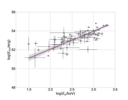
Figure 1: Cosmology-dependent fit of the Amati correlation obtained with the data in Table 1 assuming a standard flat cosmology with parameter values $h=0.674\pm 0.005$, and $\Omega_{m}=0.315\pm 0.007$ (Planck Collaboration et al., 2018). Note we have performed the corresponding error propagation to calculate the uncertainties for $E_{\rm iso}$. In this case, the parameters of the Amati correlation in Eq. (9) take values $A=1.9099\pm 0.2412$ and $B=48.2477\pm 0.6591$. The Spearman’s rank coefficient of the correlation is $\rho=0.7592$.

Following Amati et al. (2019), we construct a Bézier parametric curve of degree $n$ given by

$$H_{n}(z)=\sum_{d=0}^{n}\beta_{d}h_{n}^{d}(z), h_{n}^{d}\equiv\frac{n!(z/z_{m})^{d}}{d!(n-d)!}\left(1-\frac{z}{z_{m}}\right)^{n-d},$$ (4)

where $\beta_{d}$ are coefficients of the linear combination of Bernstein basis polynomials $h_{n}^{d}(z)$, positive in the range $0\leq z/z_{m}\leq 1$, with $z_{m}$ the maximum $z$ in the dataset employed. Specifically, we use Hubble parameter data reported by Capozziello et al. (2018), which comes from the Cosmic Chronometers (CC) approach (Jimenez & Loeb, 2002; Moresco, 2015), to build a Bézier curve of degree $n=2$ in order to obtain a monotonic growing function in such way that the Hubble constant, $H_{0}$, can be identified with the parameter $\beta_{0}$ by setting $d=0$ and $z=0$.

Cosmic Chronometers is a cosmology-independent technique to measure the Hubble parameter as a function of redshift, $H(z)$, from the differential evolution of massive and passive early-type galaxies. The strength of the CC approach is to provide a direct estimation of the expansion history of the Universe without relying on any cosmological assumption; however, the systematic uncertainties must be carefully taken into account. Such uncertainties are mostly attributed to four sources: the dependence on the stellar population synthesis (SPS) model used to calibrate the measurement, the dependence on the estimate of the stellar metallicity of the population, the dependence on the assumed model of star formation history (SFH), and finally the influence of a possible residual star formation due to a young sub-dominant component underlying the selected sample (Moresco et al., 2020). An initial estimation of the impact of systematic uncertainties was presented by Moresco et al. (2012) and Moresco et al. (2016), where the impact of the SFH assumption in the method was estimated to be $2.5\%$ on average. A more recent work showed that it is possible to minimize the impact of a recent burst of star formation through a careful selection of purely passively evolving galaxies from the optical spectra alone (Moresco et al., 2018).

Here we follow the latest analysis of Moresco et al. (2020), where the systematic uncertainties due to the choice of the stellar population synthesis model (i.e., stellar physics models, along with an adopted stellar library, initial mass function, etc.), and metallicity were estimated. The authors showed that the most relevant effects come from the SPS model, the stellar libraries and metallicity. In order to assess the impact of these systematic uncertainties in our calibration (and in our analysis of the cosmological models), we added to the measurement error of the Hubble parameter dataset we take from Capozziello et al. (2018), in quadrature, the maximum bias reported in Table 4 of Moresco et al. (2020) due to the stellar library ($7.40\%$), SPS model ($15.86\%$) and due to $5\%$ error on metallicity ($6.97\%$), that is,

$$\sigma_{\rm syst}=\pm 7.40\%({\rm StellarLib})\pm 15.86\%({\rm SPS})\pm 6.97\%({\rm met}).$$ (5)

For consistency, and given that the analysis of Moresco et al. (2020) was carried out through simulations in the redshift range $0<z<1.5$, we limit our CC Hubble data to this range and instead of using the 31 measurements of $H(z)$ reported by Capozziello et al. (2018), we work with a sub-sample of 28 measurements of Hubble parameter with maximum redshift $z=1.43$.

By employing the sub-sample of 28 measurements of the Hubble parameter, we performed a non-linear least-squares minimization by using the Python software package lmfit (Newville et al., 2014) with two error sets. In the first case, presented only for reference, we use the data without adding the bias due to the systematic uncertainties. The second case takes into account the contribution of the maximum systematic error described above. We adopt this second case to perform the subsequent steps of our analysis. The best-fit parameters obtained for the Bézier fit with $n=2$ in both cases are

$$H_{2}(z)=\beta_{0}h_{2}^{0}(z)+\beta_{1}h_{2}^{1}(z)+\beta_{2}h_{2}^{2}(z),$$ (6)

where for each case,

$$\beta_{0}^{(I)}=H_{0}^{(I)}=72.81, \beta_{1}^{(I)}=77.46, \beta_{2}^{(I)}=181.71,$$

$$\beta_{0}^{(II)}=H_{0}^{(II)}=70.81, \beta_{1}^{(II)}=81.99, \beta_{2}^{(II)}=179.02.$$ (7)

The corresponding covariance matrices are,

$$\mathbf{cov}^{(I)}=\begin{bmatrix}8.58&-15.20&6.91\\ -15.20&39.39&-23.17\\ 6.91&-23.17&43.14\\ \end{bmatrix},$$

$$\mathbf{cov}^{(II)}=\begin{bmatrix}12.99&-20.07&8.88\\ -20.07&50.18&-29.92\\ 8.88&-29.926&53.76\\ \end{bmatrix},$$

with the associated errors for the parameters in (7) encoded in the diagonal terms of each matrix. The best-fit with its 1$\sigma$ confidence region for both cases are shown in each panel of Fig. 2.

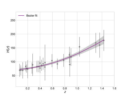
Figure 2: The 28 Hubble parameter datapoints with the fit to the Bézier curve and its respective 1$\sigma$ confidence region (shaded region). The left panel shows data with the usual errors associated to the differential age (Jimenez & Loeb, 2002) but without extra systematic errors. The right panel includes the maximum uncertainty at 1-$\sigma$ from the recent treatment of uncertainties from SPS modelling, stellar library, and stellar metallicity (Moresco et al., 2020).

The next step consists of extrapolating the function $H_{2}(z)$ to redshift $z>z_{m}$ and construct the luminosity distance $d^{\mathrm{cal}}_{L}(z)$ for a flat cosmology, that is

$$d^{\mathrm{cal}}_{L}(z)=c(1+z)\int_{0}^{z}\frac{dz^{\prime}}{H_{2}(z^{\prime})},$$ (8)

and subsequently the isotropic energy ${E^{\mathrm{cal}}_{\mathrm{iso}}=4\pi(d^{\mathrm{cal}}_{L}(z))^{2}S_{\mathrm{bolo}}(1+z)^{-1}}$. In order to obtain the corresponding errors $\sigma E^{\mathrm{cal}}_{\mathrm{iso}}$, the associated error to $\sigma^{\mathrm{cal}}_{d_{L}}$ is calculated by taking into account the correlations between the parameters $\beta$’s, see Eq. 6, besides of the GRBs systematics on the observables, $S_{\mathrm{bolo}}$. In Fig. 3, we show the corresponding $E_{\rm p}-E^{\mathrm{cal}}_{\mathrm{iso}}$ distribution, with $E^{\mathrm{cal}}_{\mathrm{iso}}$ coming from the $H(z)$ data that takes into account the maximum bias due to systematic uncertainties.

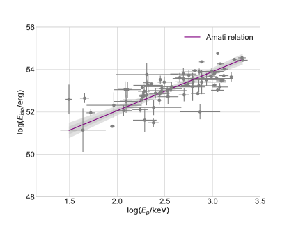
Figure 3: 74 GRBs between the redshift range $0.117\leq z\leq 5.283$. The best-fit calibration, Amati relation, is the straight line in purple. In this case the $E_{\mathrm{iso}}$ comes from the CC Hubble data that take into account the maximum extra bias. The Spearman’s rank coefficient of the correlation is $\rho=0.7623$.

To calibrate the Amati relation for our sample of 74 Fermi-GRBs, we employed the bivariate correlated errors and intrinsic scatter (BCES) method of the Python module by Nemmen et al. (2012). This fitting method performs a robust linear regression, following Akritas & Bershady (1996), which is useful when it is unclear which variable should be treated as the independent one and which as the dependent one. Moreover, the method takes into account the possible intrinsic scatter of the data with respect to the linear fit and the measurement errors in both variables.

Following this method, the best fit for the Amati relation

$$\log\left(\frac{E^{\mathrm{cal}}_{\mathrm{iso}}}{\mathrm{erg}}\right)=A\log\left(\frac{E_{\rm p}}{\mathrm{keV}}\right)+B,$$ (9)

is obtained for $A=1.8355\pm 0.2403$, $B=48.3934\pm 0.6551$, and the covariance matrix given by

$$\textbf{cov}=\left[\begin{array}[]{cccc}0.0577&-0.1568\\ -0.1568&0.4292\\ \end{array}\right].$$ (10)

It should be noted that while we used the BCES-orthogonal regression algorithm to perform our data-fitting, there are other methods of fitting Eq. (9) to our sample of GRBs. For example, we also considered the scipy.odr package, translated from the Fortran-77 odrpack by Boggs et al. (1989). odrpack is a weighted orthogonal distance regression function which takes into account errors in both variables by minimizing the weighted orthogonal distance between the observations and model. With this algorithm, the best fit to the Amati relation was estimated to be $A=1.9287\pm 0.1862$, $B=48.0725\pm 0.5321$. While this estimate agrees with our results from BCES-orthogonal method and with the results of Amati et al. (2019), some issues with the values of uncertainties on the parameters have been noted in Beatty et al. (2019); Baxter, Claire et al. (2020). Similar complications have been noted in other methods like the BCES-bisector (Hogg et al., 2010), thus we employ only the results obtained through the BCES-orthogonal method, which has been chosen as a favoured method in other applications (see e.g. Richard-Laferrière et al. (2020)).

Finally, the GRBs distance moduli, from the definition $\mu_{\mathrm{GRB}}=5\log(d_{L}^{\mathrm{cal}}/\mathrm{Mpc})+25$, can be calculated by using all the fitting parameters obtained from the Amati relation for the sample of 74 GRBs with $0.117\leq z\leq 5.283$. The variance of $\mu$ is computed by using error propagation method and is given by

$$\begin{split}\sigma_{\mu_{\mathrm{GRB}}}^{2}=&\left(\frac{\partial\mu_{\mathrm{GRB}}}{\partial A}\right)^{2}\sigma_{A}^{2}+\left(\frac{\partial\mu_{\mathrm{GRB}}}{\partial B}\right)^{2}\sigma_{B}^{2}+\\ &2\left(\frac{\partial\mu_{\mathrm{GRB}}}{\partial A}\right)\left(\frac{\partial\mu_{\mathrm{GRB}}}{\partial B}\right)\sigma_{AB}+\left(\frac{\partial\mu_{\mathrm{GRB}}}{\partial E_{\rm p}}\right)^{2}\sigma_{E_{\rm p}}^{2}\\ &+\left(\frac{\partial\mu_{\mathrm{GRB}}}{\partial S_{\mathrm{bolo}}}\right)^{2}\sigma_{S_{\mathrm{bolo}}}^{2},\end{split}$$ (11)

where the covariances for $E_{\rm p}$ and $S_{\mathrm{bolo}}$ are absent since they are not correlated.

The distance moduli of the 74 GRBs, $\mu_{\mathrm{GRB}}$, and their 1$\sigma$ uncertainties calibrated through the Amati relation are listen in Table 2. The corresponding distribution of $\mu_{\mathrm{GRB}}$ versus $z$ is shown in Fig. 4 together the most recent compilation of SNe Ia, the Pantheon dataset (Scolnic et al., 2018).

Name	$z_{\mathrm{GRB}}$	$\mu_{\mathrm{GRB}}$	$\sigma_{\mu_{\rm GRB}}$
GRB180728728	0.117	40.2876	0.485068
GRB150727793	0.313	43.5373	0.38344
GRB171010792	0.3285	39.7107	0.309248
GRB130427324	0.34	42.2947	0.245225
GRB130925173	0.347	37.6941	0.751191
GRB140606133	0.384	45.7371	0.455169
GRB190114873	0.425	43.3469	0.27912
GRB091127976	0.4903	41.2349	0.620159
GRB090618353	0.54	41.0103	0.261624
GRB170607971	0.557	43.5656	0.358325
GRB141004973	0.573	43.2978	0.923718
GRB130215063	0.597	42.8165	0.442175
GRB131231198	0.642	42.7956	0.213511
GRB161129300	0.645	44.3482	0.630753
GRB180720598	0.654	44.6778	0.239499
GRB080916406	0.689	43.0348	0.497411
GRB111228657	0.7163	40.2065	0.658414
GRB140512814	0.725	45.4356	0.310337
GRB160804065	0.736	42.6363	0.417647
GRB090328401	0.736	45.7377	0.283133
GRB100816026	0.8049	46.7315	0.288428
GRB150514774	0.807	43.877	0.454466
GRB151027166	0.81	43.5722	0.297084
GRB091003191	0.8969	45.7004	0.218752
GRB141225959	0.915	44.6923	0.28191
GRB140508128	1.027	44.5137	0.172955
GRB091208410	1.0633	43.4901	0.741808
GRB180620660	1.1175	44.2046	0.589936
GRB160509374	1.17	42.8561	0.186522
GRB190324947	1.1715	44.5738	0.250219
GRB140213807	1.2076	44.109	0.314352
GRB090926914	1.24	44.214	0.312897
GRB130420313	1.297	42.6682	0.430143
GRB140801792	1.32	45.6352	0.225935
GRB100414097	1.368	46.448	0.326704
GRB100615083	1.398	43.0109	0.481797
GRB160625945	1.406	43.0984	0.251807
GRB100814160	1.44	43.957	0.239648
GRB180314030	1.445	44.8533	0.253852
GRB110213220	1.46	45.1038	0.305649
GRB161117066	1.549	43.387	0.29187
GRB100728095	1.567	44.3048	0.165154
GRB100906576	1.727	42.6846	0.705178
GRB120119170	1.728	45.004	0.184931
GRB150314205	1.758	45.9886	0.220605
GRB120326056	1.798	44.9544	0.475731
GRB131011741	1.874	45.9691	0.404528
GRB170705115	2.01	45.4027	0.259356
GRB161017745	2.0127	46.8726	0.379906
GRB140620219	2.04	44.4257	0.413362
GRB150403913	2.06	46.9528	0.298582
GRB090926181	2.1062	46.3678	0.234238
GRB120624933	2.1974	45.88	0.392779
GRB121128212	2.2	45.114	0.324018
GRB081221681	2.26	44.5865	0.216956
GRB141028455	2.33	46.7664	0.251315
GRB130518580	2.49	46.6589	0.295154
GRB081121858	2.512	45.6925	0.231653
GRB170214649	2.53	46.0353	0.344863
GRB120811649	2.671	46.1205	0.319856
GRB140206304	2.74	45.7267	0.177794
GRB081222204	2.77	46.8751	0.185688
GRB110731465	2.83	48.1874	0.288535
GRB181020792	2.938	46.9983	0.256644
GRB140703026	3.14	47.5843	0.385486
GRB140423356	3.26	45.8838	0.309091
GRB140808038	3.29	48.4009	0.196729
GRB110818860	3.36	47.4237	0.659063
GRB170405777	3.51	46.6516	0.27214
GRB090323002	3.57	47.3263	0.402843
GRB120909070	3.93	47.3737	0.328148
GRB090516353	4.109	46.9323	0.407857
GRB120712571	4.1745	48.4067	0.310428
GRB140304557	5.283	48.7986	0.542238

Table 2: Distance moduli of 74 GRBs calibrated through the Amati relation.

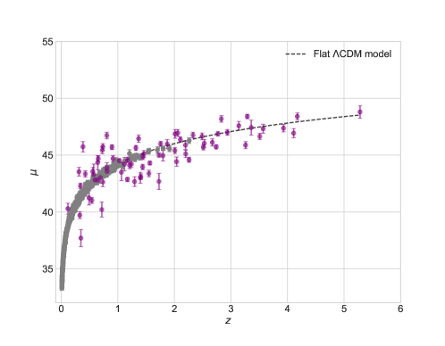
Figure 4: Distance moduli $\mu_{\mathrm{GRB}}$ for our 74 GRB sample together with the SNe Ia distance moduli compared to the flat $\Lambda$CDM model with $\Omega_{m}=0.315$ and $h=0.674$.

Before we proceed, we stress that, although there is a debate as to whether the Amati relation is an intrinsic effect, or the result of detection biases, or even a combination of these two (Butler et al., 2007; Li, 2007b; Ghirlanda et al., 2008; Butler et al., 2009, 2010; Collazzi et al., 2012; Kocevski, 2012; Heussaff et al., 2013; Petrosian et al., 2015). Other works have claimed that the instrumental selection biases, even if they may affect the sample, cannot be responsible for the existence of the spectral-energy correlations Ghirlanda et al. (2008); Nava et al. (2012b). Additionally, the Amati relation could arguably change with redshift, but previous analyses have shown the opposite based on current data (e.g., Demianski et al. (2017b)). More thorough discussions supporting the reliability of Amati relation can be found in Demianski et al. (2017a); Dainotti & Amati (2018); Dirirsa et al. (2019)

4 Dark Energy models

The dark energy dominance induces a period of accelerated expansion, well described by an effective equation of state $\omega_{\rm DE}=p_{\rm DE}/\rho_{\rm DE}$ (the label ${\rm DE}$ stands for dark energy). In the homogeneous and isotropic (FLRW) description of the Universe, a negative pressure (specifically $\omega_{\rm DE}<-1/3$) is required in order to induce the accelerated expansion. Furthermore, the parameter $\omega_{\rm DE}$ determines the gravitational properties of dark energy as well as its own evolution, derived from the energy-momentum conservation. The Friedmann equation (field equation) assuming a flat cosmology, pressureless matter, and negligible radiation is,

$$\frac{H^{2}(z)}{H^{2}_{0}}=\Omega_{m}(1+z)^{3}+\Omega_{\rm DE}\exp{\left(3\int\frac{dz^{\prime}}{1+z^{\prime}}[1+\omega_{\rm DE}(z^{\prime})]\right)},$$ (12)

where the density fraction parameters are defined as $\Omega_{m}\equiv\rho_{m}(t_{0})/\rho_{c}^{0}$ and $\Omega_{\rm DE}\equiv\rho_{\rm DE}(t_{0})/\rho_{c}^{0}$ with critical density $\rho_{c}^{0}\equiv 3H_{0}^{2}/(8\pi G)$. It is important to recall that in this work $H_{0}$ is not a parameter constrained by the Bayesian analysis. This is because once we fit the Bezier curve, the value for the Hubble constant is set through the $\beta_{0}$ parameter (see Eq. (7)).

From Eq. (12), we recover the expansion history for all the dark energy models here studied:

1. $\Lambda$CDM model

   In this case Eq. (12) reads,

   $$H^{2}(z)=H^{2}_{0}\left[\Omega_{m}(1+z)^{3}+\Omega_{\rm DE}\right],$$ (13)

   where $\Omega_{\Lambda}\equiv\Omega_{\rm DE}$ is the density fraction due to a cosmological constant with equation of state $\omega_{\Lambda}=-1$. Requiring the consistency of Eq. (13) at $z=0$, that is, $H(z=0)=H_{0}$, yields $\Omega_{m}+\Omega_{\Lambda}=1$. Thus, there is only one free parameter.

2. $\omega$CDM model

   For the case in which $\omega_{\rm DE}$ is a constant such that $\omega_{\rm DE}\equiv\omega_{0}\neq-1$, one gets

   $$H^{2}(z)=H^{2}_{0}\left[\Omega_{m}(1+z)^{3}+\Omega_{\rm DE}(1+z)^{3(1+\omega_{\rm DE})}\right],$$ (14)

   where $\Omega_{\rm DE}$ is the density fraction due to the dark energy fluid. Since flatness imposes the constraint $\Omega_{m}+\Omega_{\rm DE}=1$, then the free parameters of this model are $\Omega_{m}$ and $\omega_{0}$.

3. CPL model

   In the well-known CPL model, the equation of state is $\omega_{\rm DE}=\omega_{0}+\omega_{a}\frac{z}{1+z}$, where $\omega_{0}$ and $\omega_{a}$ are both constants. The Hubble parameter equation, from Eq. (12), is

   $$H^{2}(z)=H^{2}_{0}\left[\Omega_{m}(1+z)^{3}+\Omega_{\rm DE}(1+z)^{3(1+\omega_{0}+\omega_{a})}\exp{\left(-\frac{3\omega_{a}z}{1+z}\right)}\right],$$ (15)

   where $\Omega_{\rm DE}$ is the density fraction due to the dark energy fluid and again $\Omega_{m}+\Omega_{\rm DE}=1$ is imposed. Consequently, the free parameters of the model are $\Omega_{m}$, $\omega_{0}$ and $\omega_{a}$.

Our task is to constrain the free parameters of each model by performing a Bayesian parameter estimation on the a set of up-to-date observations, including Type Ia Supernovae, BAO data and CMB data in the condensed form of shift parameters, complementing the GRB distance moduli reported here.

5 Parameter estimation of Dark Energy Models

We have used the public Boltzmann code class (Lesgourgues, 2011) to run the background evolution for all the dark energy models studied here. Then we use the cosmological parameter estimator monte python (Audren et al., 2013), which is linked to class and adopts the Markov Chain Monte Carlo (MCMC) method to constrain the parameters of each DE model by fitting the cosmological data. The code employs the Metropolis-Hastings algorithm (Metropolis et al., 1953; Hastings, 1970) for sampling, and computes the Bayesian parameter inference of the posteriors with the convergence test given by the Gelman-Rubin criterion $R$ (Gelman & Rubin, 1992), where the condition $R-1<10^{-3}$ is imposed to end all of our chains.

In addition to the calibrated samples of Gamma Ray Bursts listed above, the suite of datasets considered for our analysis includes those related to the expansion history of the universe (described by Eq. (12)), i.e., the ones describing the distance-redshift relations as detailed below.

5.1 Observational data

5.1.1 Type Ia Supernovae (SNe Ia)

One of the latest SNe Ia data compilation is the Pantheon sample (Scolnic et al., 2018) which consists of 1048 SNe with the redshift spanning $0.01<z<2.3$. This sample is a combination of 365 spectroscopically confirmed SNe Ia discovered by the Pan-STARRS1(PS1) Medium Deep Survey together with the subset of 279 PS1 SNe Ia ($0.03<z<0.68$) with distance estimates from SDSS, SNLS and several low-$z$ and Hubble Space Telescope samples (see Table 4 of Scolnic et al. (2018)). In order to include this data, we define

$$\chi^{2}_{SN}=\mathrm{\Delta}\mathrm{\mu^{SN}}\cdot\mathrm{C_{SN}^{-1}}\cdot\mathrm{\Delta}\mathrm{\mu^{SN}},$$ (16)

where $\mathrm{C_{SN}}$ is the full systematic covariance matrix and $\mathrm{\Delta}\mathrm{\mu^{SN}}=\mathrm{\mu_{theo}}-\mathrm{\mu_{obs}}$ is the vector of the differences between the observed and theoretical value of the distance modulus, $\mathrm{\mu}$, with the absolute magnitude taken as nuisance parameter.

5.1.2 Baryon Acoustic Oscillations (BAO)

Survey	$z_{\mathrm{BAO}}$	Measurement
6DF	$0.106$	$r_{\mathrm{s}}/D_{V}$
SDSS DR7 MGS	$0.15$	$D_{V}/r_{\mathrm{s}}$
SDSS DR12 galaxies	$0.38$, $0.51$, $0.61$	$D_{A}/r_{\mathrm{s}}$, $D_{H}/r_{\mathrm{s}}$

Table 3: BAO measurements from various surveys, Beutler et al. (2011); Ross et al. (2015); Alam et al. (2017), adopted in this work.

We used the low redshift galaxy BAO data listed in Table 3. The data provide measurements of three types of ratios of comoving distance: the angular scale of the BAO ($D_{A}(z)/r_{\mathrm{s}}$), the redshift-space BAO scale ($D_{H}(z)/r_{\mathrm{s}}$), with $D_{H}(z)=c/H(z)$  (Alam et al., 2017), and the spherically-averaged BAO scale ($D_{V}(z)/r_{\mathrm{s}}$) (Beutler et al., 2011; Ross et al., 2015). Here $r_{\mathrm{s}}$ is the comoving sound horizon at the end of the baryon drag epoch, given by

$$r_{\mathrm{s}}=\int_{z_{d}}^{\infty}\frac{c_{s}(z)}{H(z)}dz,$$ (17)

where $c_{s}$ denotes the sound speed in the primordial photon-baryon plasma given by $c_{s}=3^{-1/2}c[1+\frac{3}{4}\rho_{b}(z)/\rho_{\gamma}(z)]^{-1/2}$. $D_{A}(z)$ is the comoving angular diameter distance

$$D_{A}(z)=c\int_{0}^{z}\frac{dz^{\prime}}{H(z^{\prime})},$$ (18)

and $D_{V}(z)$ is the spherically averaged combination of transverse and radial BAO modes,

$$D_{V}(z)=\left[zD_{H}(z)D_{A}^{2}(z)\right]^{1/3}.$$ (19)

Thus, the corresponding $\chi_{BAO}^{2}$ for BAO data is given by

$$\chi^{2}_{BAO}=\mathrm{\Delta}\mathbfcal{F}^{BAO}\cdot\mathbf{C}_{BAO}^{-1}\cdot\mathrm{\Delta}\mathbfcal{F}^{BAO},$$ (20)

where $\mathrm{\Delta}\mathbfcal{F}^{BAO}=\mathcal{F}_{theo}-\mathcal{F}_{obs}$ is the difference between the observed and theoretical value of the observable quantity for BAO, which may vary from one survey to another, and $\mathbf{C}^{-1}_{BAO}$ is the respective inverse covariance matrix.

5.1.3 Cosmic Microwave Background (CMB)

Instead of the full data of the CMB anisotropies, we use CMB data in the condensed form of shift parameters reported by Chen et al. (2019), derived from the last release of the Planck results (Planck Collaboration et al., 2018). Evidently, the analysis proceeds much faster in this way than by performing an analysis involving the full CMB likelihood.

As argued by several authors, the shift parameters $(R,l_{A},\Omega_{b}h^{2},n_{s})$ provide an efficient summary of CMB data as far as DE constraints are concerned (Kosowsky et al., 2002; Wang & Mukherjee, 2007; Mukherjee et al., 2008; Ade et al., 2016). This set of parameters can be used to study models with either non-zero curvature or a smooth DE component, as is our case, but not with modifications of gravity (Mukherjee et al., 2008; Ade et al., 2016).

The first two quantities in the vector $(R,l_{A},\Omega_{b}h^{2},n_{s})$ are defined as

$$R\equiv\sqrt{\Omega_{m}H_{0}^{2}}\frac{r(z_{*})}{c},$$ (21)

$$l_{A}\equiv\pi\frac{r(z_{*})}{r_{s}(z_{*})},$$ (22)

where $r(z)$ is the comoving distance, here evaluated at photon-decoupling epoch $z_{*}$. The corresponding $\chi^{2}$ for the CMB is thus

$$\chi^{2}_{CMB}=\mathrm{\Delta}\mathbfcal{F}^{CMB}\cdot\mathbf{C}_{CMB}^{-1}\cdot\mathrm{\Delta}\mathbfcal{F}^{CMB},$$ (23)

where $\mathcal{F}^{CMB}=(R,l_{A},\Omega_{b}h^{2},n_{s})$ is the vector of the shift parameters and $\mathbf{C}^{-1}_{CMB}$ is the respective inverse covariance matrix. The mean values for these shift parameters as well as their standard deviations and normalized covariance matrix are taken from Table 1 of Chen et al. (2019).

5.1.4 Gamma-Ray Bursts (GRBs)

We test our method by analysing two samples. The first one consists on 193 GRBs calibrated in Amati et al. (2019) which cover the redshift range $0.03351\leq z\leq 8.1$. The second sample is our set of 74 Fermi-GRBs, a selection described in detail above, with a redshift range $0.117\leq z\leq 5.283$.

The $\chi^{2}$ function for the GRBs data is defined analogous to Eq. (16) of SNe Ia data, that is,

$$\chi^{2}_{GRB}=\mathrm{\Delta}\mathrm{\mu}^{GRB}\cdot\mathrm{C^{-1}}_{GRB}\cdot\mathrm{\Delta}\mathrm{\mu}^{GRB},$$ (24)

where $\mathrm{C}_{GRB}$ is a diagonal matrix containing $\sigma^{2}_{\mu}$ and $\mathrm{\Delta}\mathrm{\mu}^{GRB}=\mathrm{\mu_{theo}}-\mathrm{\mu_{estimated}}$ is the vector of the differences between the theoretical and estimated value of the distance moduli for the GRBs.

6 RESULTS

We have obtained the constraints for the $\Lambda$CDM, $\omega$CDM and CPL models from the latest observational data of SNe Ia, BAO, CMB distance priors inferred from the final Planck 2018 data, and including either the 193 GRBs calibrated by Amati et al. (2019) labeled as sample (1) or the 74 GRBs calibrated in this work labeled as sample (2-nosys) or sample (2-sys). For comparison, SNe Ia + BAO + CMB without GRBs have been also analysed in order to highlight the contribution of GRBs to the joint cosmological constraints.

We used flat priors for the free parameters of the models analyzed with ranges set as follow: $\Omega_{m}\in(0.1,0.5)$ (all models). $\omega_{0}$ in the $\mathrm{\omega CDM}$ model with no priors. Finally, the CPL parameters are allowed to take values in the ranges $\omega_{0}\in(-2,0),~{}\omega_{a}\in(-5,5)$. Note that if we wanted to constraint the value for the Hubble constant $H_{0}$ from all cosmological data employed in this work, it would be necessary to leave $\beta_{0}$ as a free parameter before and after the Bezier function fitting.

	SNIa+BAO+CMB		SNIa+BAO+CMB + GRBs(1)		ALL + GRBs(2-no sys)		ALL + GRBs(2-sys)
	best-fit	mean$\pm\sigma$	best-fit	mean$\pm\sigma$	best-fit	mean$\pm\sigma$	best-fit	mean$\pm\sigma$
$\Omega_{\mathrm{m}}$	$0.3179$	$0.3179_{-0.00058}^{+0.00057}$	$0.3180$	$0.3180_{-0.00057}^{+0.00057}$	$0.3180$	$0.3180_{-0.00057}^{+0.00057}$	$0.3180$	$0.3180_{-0.00057}^{+0.00057}$

Table 4: Constraints at 68$\%$ C.L. on the cosmological parameter $\Omega_{\mathrm{m}}$ in case of the $\Lambda$CDM model using different combinations of datasets. 1) The joint analysis of the SNe Ia, BAO and CMB distance priors, 2) SNe Ia + BAO + CMB + the sample of 193 GRBs calibrated by Amati et al. (2019), labeled as GRBs(1). For 3) and 4) SNe Ia + BAO + CMB is condensed as ALL and the sample of 74 GRBs from Fermi-GBM catalog calibrated in this work, labeled as GRBs(2-no sys) and GRBs(2-sys) without and with extra bias in the CC Hubble data, respectively, is added.

In Table 4, the best-fit values for $\Omega_{m}$ with 1-$\sigma$ uncertainties are shown. In spite of the relatively large dispersion observed in our calibrated GRBs sample, the results obtained by using either GRBs(2-nosys) or GRBs(2-sys) plus SNIa+BAO+CMB are in good agreement with the results we obtained by using the calibrated sample by Amati et al. (2019), namely the results obtained by using SNIa+BAO+CMB+GRBs(1), and these are consistent with the Planck 2018 results (Planck Collaboration et al., 2018) at 1$\sigma$ confidence level.

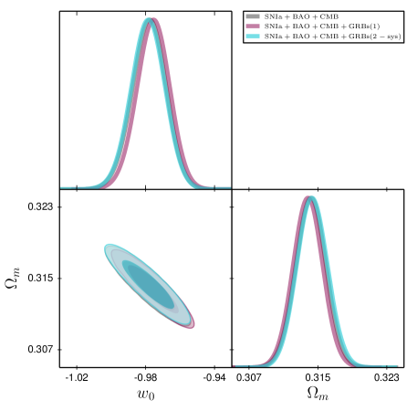
Figure 5: Constraints at the 68$\%$ and 95$\%$ C.L. on the ($\omega_{0}$, $\Omega_{\mathrm{m}}$) plane from the combinations of datasets 1) The joint analysis of the SNe Ia, BAO and CMB distance priors, 2) SNe Ia + BAO + CMB + the sample of 193 GRBs calibrated by Amati et al. (2019), labeled as GRBs(1) and 3) SNe Ia + BAO + CMB + the sample of 74 GRBs from Fermi-GBM catalog presented in this work taking into account extra bias due to the systematic uncertainties in the CC Hubble dataset, labeled as GRBs(2-sys).

	SNe Ia + BAO + CMB		SNe Ia + BAO + CMB + GRBs(1)		ALL + GRBs (2- no sys)		ALL + GRBs (2- sys)
	best-fit	mean$\pm\sigma$	best-fit	mean$\pm\sigma$	best-fit	mean$\pm\sigma$	best-fit	mean$\pm\sigma$
$\omega_{0}$	$-0.9776$	$-0.9782_{-0.0096}^{+0.01}$	$-0.9755$	$-0.9757_{-0.0096}^{+0.0099}$	$-0.9783$	$-0.9785_{-0.0097}^{+0.01}$	$-0.9779$	$-0.9786_{-0.0098}^{+0.01}$
$\Omega_{\mathrm{m}}$	$0.3141$	$0.3142_{-0.0018}^{+0.0018}$	$0.3138$	$0.3138_{-0.0018}^{+0.0018}$	$0.3143$	$0.3143_{-0.0018}^{+0.0018}$	$0.3142$	$0.3144_{-0.0018}^{+0.0018}$

Table 5: Constraints at 68$\%$ C.L. on the cosmological parameters of the $\omega$CDM model using the combinations of datasets mentioned in Table 4.

The results of a similar analysis for the two parameters of the $\omega$CDM model are displayed in Figure 5. We show only the results from the calibrated sample of GRBs that comes from the inclusion of extra bias in the CC Hubble dataset. In this case our calibrated sample yields a value for the $\omega_{0}$ parameter consistent with the ones obtained from the other datasets employed here.

The corresponding best-fits of the analysis are listed in Table 5. It is important to note that the parameter estimation of Amati et al. (2019) for this model yields best fit values for $\omega_{0}$ that fall far from our fit of their same dataset and show a much larger uncertainty than ours.

This advocates for our method as an improvement over previous analyses of GRB data.

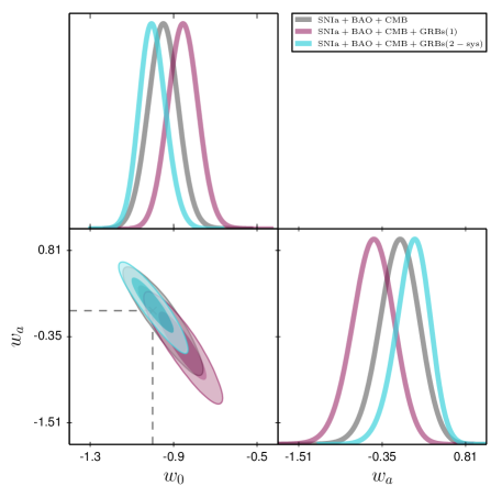
Figure 6: Constraints at the 68$\%$ and 95$\%$ C.L. on the ($\omega_{0}$, $\omega_{a}$) plane from the combinations of datasets mentioned in Fig. 5.

	SNe Ia + BAO + CMB		SNe Ia + BAO + CMB + GRBs(1)		ALL + GRBs(2-no sys)		ALL + GRBs(2- sys)
	best-fit	mean$\pm\sigma$	best-fit	mean$\pm\sigma$	best-fit	mean$\pm\sigma$	best-fit	mean$\pm\sigma$
$\omega_{0}$	$-0.9631$	$-0.9515_{-0.078}^{+0.074}$	$-0.8628$	$-0.8548_{-0.075}^{+0.073}$	$-1.002$	$-0.9933_{-0.069}^{+0.066}$	$-1.009$	$-0.9982_{-0.068}^{+0.064}$
$\omega_{a}$	$-0.05507$	$-0.1079_{-0.27}^{+0.3}$	$-0.4361$	$-0.4782_{-0.28}^{+0.31}$	$0.09276$	$0.05013_{-0.23}^{+0.27}$	$0.1135$	$0.06781_{-0.22}^{+0.26}$
$\Omega_{\mathrm{m}}$	$0.3142$	$0.3144_{-0.0019}^{+0.0018}$	$0.3144$	$0.3147_{-0.0019}^{+0.0018}$	$0.3139$	$0.3142_{-0.0019}^{+0.0018}$	$0.3141$	$0.3143_{-0.0019}^{+0.0018}$

Table 6: Constraints at 68$\%$ C.L. on the cosmological parameters of the CPL model using the combinations of datasets mentioned in Table 4.

In Figure 6 we show 1$\sigma$ (dark colours) and 2$\sigma$ (light colours) error contours in the ($\omega_{0}$, $\omega_{a}$) parameter-space of the CPL model, resulting from the combination of samples indicated above. The datasets tested for this model show consistency in parameter values at $1\sigma$. Furthermore, the parameter values fitting the new sample of GRBs favours the $\Lambda$CDM model more than the other two cases. This is clear from Table 6, where the $\Lambda$CDM values $(\omega_{0}=-1,\omega_{a}=0)$ lie close to the central values of our new GRBs dataset.

We also note that the values of the parameter $\omega_{0}$ in the CPL model from the three datasets employed in this work, intersect the range of values resulting from the Planck 2018 data at 1$\sigma$ (Planck Collaboration et al., 2018), in contrast with the recent results of Demianski et al. (2019) (where a sample of GRBs covering a redshift range of $0.033\leq z<9$ is employed, together with direct $H(z)$ measurements (Farooq & Ratra, 2013) and the past compilation of SNe Ia Union 2.1 (Suzuki et al., 2012)). We emphasise that our adequate handling of errors, and a suitable choice of calibration method, yield a significantly tighter confidence region for the parameters of the models here presented, in comparison to the posteriors of previous works.

For a quick insight into model comparison, we compute the Bayesian information criterion (BIC) introduced by Schwarz (1978), defined as

$$BIC=-2\ln{\mathcal{L_{\mathrm{max}}}}+k\ln{N},$$ (25)

where $N$ is the number of datapoints used in the fit and $k$ is the number of free parameters of the cosmological model. In practice, one computes BIC for each of the candidate models and selects the model of reference to calculate the difference $\Delta\mathrm{BIC}=\Delta\chi^{2}+\Delta k\ln N$. A difference in $\Delta\mathrm{BIC}$ of 2 is considerable positive evidence against the model with higher BIC, while a $\Delta\mathrm{BIC}$ of 6 is considered to be strong evidence Jeffreys (1961). For the model comparison we choose the $\Lambda$CDM model as the model of reference because it shows lowest BIC score. Thus, for the case in which our calibrated sample of GRBs is coming from CC Hubble data with extra systematics uncertainties, we obtained $\Delta\mathrm{BIC}_{\mathrm{\omega CDM}}=2.25$ and $\Delta\mathrm{BIC}_{\mathrm{CPL}}=9.08$ indicating positive evidence against $\omega$CDM model and strong evidence against the CPL model. The evidence against alternative models is slightly weaker when our GRBs sample is removed, in this case we found $\Delta\mathrm{BIC}_{\mathrm{\omega CDM}}=1.97$ and $\Delta\mathrm{BIC}_{\mathrm{CPL}}=8.88$ showing a positive weak evidence against the $\omega$CDM but confirming the strong evidence against the CPL model. Thus, by employing the BIC selection criteria to compare the statistical performance of all the studied models with and without our calibrated sample of GRBs, we found that $\Lambda$CDM model is still preferred with respect to the $\omega$CDM and CPL models.

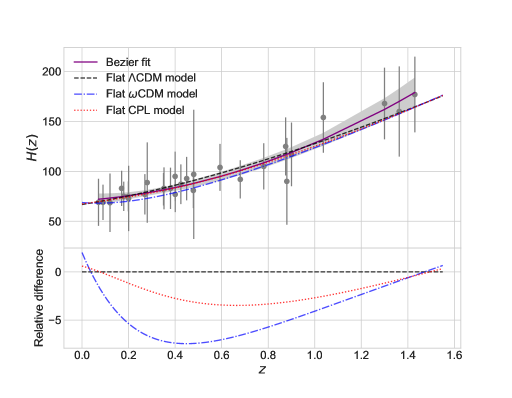
Figure 7: In the upper panel, the 28 Hubble parameter datapoints with the fit to the Bézier curve and its respective 1$\sigma$ confidence region (shaded region including the maximum uncertainty at 1-$\sigma$ from the recent treatment of uncertainties from SPS modelling, stellar library, and stellar metallicity (Moresco et al., 2020). Additionally, the fitted Hubble function for each of the cosmological models constrained in this paper are shown. In the lower panel, the relative differences of the models w.r.t. the $\Lambda$CDM one.

7 Conclusions and Discussion

Through the criteria described in Sec. 2 we have carefuly selected a sample of 74 GRBs as tracers of the luminosity distance. The Amati relation for these GRBs is calibrated in a model-independent way. Such calibration, described in Section 3, relies on $H(z)$ data coming from the CC approach as our calibration source at low redshifts.

We have computed and incorporated our GRB distance moduli to a suite of observations complemented by the latest CMB, BAO and SNe 1a data in order to fit parameters of Dark Energy and test the usefulness of our sample. We find consistency with previous works for $\Lambda$CDM and $\omega$CDM models at 1$\sigma$ in the posterior contours of the relevant parameters, with the bonus of a much tighter confidence region for the parameters. This is particularly evident for the CPL model, where the preferred values are close to those of $\Lambda$CDM, in contrast to recent results in the literature (Demianski et al., 2019)

Since the parameter values of alternative models and the BIC criterion suggest preference of a $\Lambda$CDM cosmology, we argue that this is still the better model to describe all of the data.

There is room for improvement in the analysis here presented. Most prominently, the Bezier fit to the CC Hubble data is not reproduced by the $H(z)$ function of the cosmological models as shown in Figure 7. This means that the cosmology dictated by the CC Hubble data is not reproduced in the posterior values of the tested models. As an alternative proposal to circumvent the circularity problem, one might find convergence by jointly calibrating the GRB Amati relation and the fitting to the cosmological model, including the CC Hubble data as one more set of observations (Firmani et al., 2006b, 2005; Xu et al., 2005; Schaefer, 2007; Li, 2007a). We shall perform these alternative tests and compare strategies to tackle the circularity problem in a follow-up study.

In the meantime, given the reduction of the confidence region in the parameter space of alternative models obtained from our GRB sample and method, we argue in favour of our analysis when considering GRBs and other luminosity distance probes.

Data availability

The data underlying this article are available in the article.

References

- Ade et al. (2016) Ade P. A. R., et al., 2016, Astron. Astrophys., 594, A14
- Akaike (1974) Akaike H., 1974, in , Selected Papers of Hirotugu Akaike. Springer, pp 215–222
- Akritas & Bershady (1996) Akritas M. G., Bershady M. A., 1996, Astrophys. J., 470, 706
- Alam et al. (2017) Alam S., et al., 2017, Mon. Not. Roy. Astron. Soc., 470, 2617
- Amati & Della Valle (2013) Amati L., Della Valle M., 2013, Int. J. Mod. Phys., D22, 1330028
- Amati et al. (2002) Amati L., et al., 2002, Astron. Astrophys., 390, 81
- Amati et al. (2008) Amati L., Guidorzi C., Frontera F., Della Valle M., Finelli F., Landi R., Montanari E., 2008, Mon. Not. Roy. Astron. Soc., 391, 577
- Amati et al. (2019) Amati L., D’Agostino R., Luongo O., Muccino M., Tantalo M., 2019, Mon. Not. Roy. Astron. Soc., 486, L46
- Atwood et al. (2009) Atwood W. B., et al., 2009, ApJ, 697, 1071
- Audren et al. (2013) Audren B., Lesgourgues J., Benabed K., Prunet S., 2013, JCAP, 1302, 001
- Band et al. (1993) Band D., et al., 1993, ApJ, 413, 281
- Baxter, Claire et al. (2020) Baxter, Claire et al., 2020, A&A, 639, A36
- Beatty et al. (2019) Beatty T. G., Marley M. S., Gaudi B. S., Colón K. D., Fortney J. J., Showman A. P., 2019, AJ, 158, 166
- Betoule et al. (2014) Betoule M., et al., 2014, Astron. Astrophys., 568, A22
- Beutler et al. (2011) Beutler F., et al., 2011, mnras, 416, 3017
- Boggs et al. (1989) Boggs P. T., Donaldson J. R., Byrd R. h., Schnabel R. B., 1989, ACM Trans. Math. Softw., 15, 348–364
- Bretón & Montiel (2013) Bretón N., Montiel A., 2013, Phys. Rev., D87, 063527
- Butler et al. (2007) Butler N. R., Kocevski D., Bloom J. S., Curtis J. L., 2007, ApJ, 671, 656
- Butler et al. (2009) Butler N. R., Kocevski D., Bloom J. S., 2009, ApJ, 694, 76
- Butler et al. (2010) Butler N. R., Bloom J. S., Poznanski D., 2010, ApJ, 711, 495
- Capozziello et al. (2018) Capozziello S., D’Agostino R., Luongo O., 2018, Mon. Not. Roy. Astron. Soc., 476, 3924
- Chen et al. (2019) Chen L., Huang Q.-G., Wang K., 2019, JCAP, 1902, 028
- Collazzi et al. (2012) Collazzi A. C., Schaefer B. E., Goldstein A., Preece R. D., 2012, ApJ, 747, 39
- Coward (2009) Coward D. M., 2009, Mon. Not. Roy. Astron. Soc., 393, L65
- Cucchiara et al. (2011) Cucchiara A., et al., 2011, The Astrophysical Journal, 736, 7
- Dainotti & Amati (2018) Dainotti M. G., Amati L., 2018, Publ. Astron. Soc. Pac., 130, 051001
- Dainotti et al. (2008) Dainotti M. G., Cardone V. F., Capozziello S., 2008, Mon. Not. Roy. Astron. Soc., 391, 79
- Dainotti et al. (2018) Dainotti M., Del Vecchio R., Tarnopolski M., 2018, Adv. Astron., 2018, 4969503
- Demianski et al. (2017a) Demianski M., Piedipalumbo E., Sawant D., Amati L., 2017a, A&A, 598, A112
- Demianski et al. (2017b) Demianski M., Piedipalumbo E., Sawant D., Amati L., 2017b, Astron. Astrophys., 598, A112
- Demianski et al. (2019) Demianski M., Piedipalumbo E., Sawant D., Amati L., 2019, arXiv e-prints, p. arXiv:1911.08228
- Dirirsa et al. (2019) Dirirsa F. F., et al., 2019, Astrophys. J., 887, 13
- Farooq & Ratra (2013) Farooq O., Ratra B., 2013, Astrophys. J., 766, L7
- Fenimore & Ramirez-Ruiz (2000) Fenimore E. E., Ramirez-Ruiz E., 2000, Submitted to: Astrophys. J.
- Firmani et al. (2005) Firmani C., Ghisellini G., Ghirlanda G., Avila-Reese V., 2005, Mon. Not. Roy. Astron. Soc., 360, L1
- Firmani et al. (2006a) Firmani C., Ghisellini G., Avila-Reese V., Ghirlanda G., 2006a, Monthly Notices of the Royal Astronomical Society, 370, 185
- Firmani et al. (2006b) Firmani C., Avila-Reese V., Ghisellini G., Ghirlanda G., 2006b, Mon. Not. Roy. Astron. Soc., 372, L28
- Gehrels et al. (2004) Gehrels N., et al., 2004, ApJ, 611, 1005
- Gelman & Rubin (1992) Gelman A., Rubin D. B., 1992, Statist. Sci., 7, 457
- Ghirlanda et al. (2004a) Ghirlanda G., Ghisellini G., Lazzati D., Firmani C., 2004a, The Astrophysical Journal, 613, L13
- Ghirlanda et al. (2004b) Ghirlanda G., Ghisellini G., Lazzati D., 2004b, Astrophys. J., 616, 331
- Ghirlanda et al. (2008) Ghirlanda G., Nava L., Ghisellini G., Firmani C., Cabrera J. I., 2008, MNRAS, 387, 319
- Ghirlanda et al. (2011) Ghirlanda G., Ghisellini G., Nava L., Burlon D., 2011, MNRAS, 410, L47
- Ghirlanda et al. (2012) Ghirlanda G., et al., 2012, MNRAS, 422, 2553
- Gruber et al. (2014) Gruber D., et al., 2014, ApJS, 211, 12
- Hastings (1970) Hastings W. K., 1970, Biometrika, 57, 97
- Heussaff et al. (2013) Heussaff V., Atteia J.-L., Zolnierowski Y., 2013, Astron. Astrophys., 557, A100
- Hogg et al. (2010) Hogg D. W., Bovy J., Lang D., 2010, arXiv e-prints, p. arXiv:1008.4686
- Hsiao et al. (2020) Hsiao T. Y.-Y., et al., 2020, MNRAS, 496, 4405
- Jeffreys (1961) Jeffreys H., 1961, Theory of probability. Third edition, Clarendon Press, Oxford
- Jimenez & Loeb (2002) Jimenez R., Loeb A., 2002, The Astrophysical Journal, 573, 37
- Kaneko et al. (2006) Kaneko Y., Preece R. D., Briggs M. S., Paciesas W. S., Meegan C. A., Band D. L., 2006, ApJS, 166, 298
- Kang et al. (2020) Kang Y., Lee Y.-W., Kim Y.-L., Chung C., Ree C. H., 2020, ApJ, 889, 8
- Kocevski (2012) Kocevski D., 2012, ApJ, 747, 146
- Kodama et al. (2008) Kodama Y., Yonetoku D., Murakami T., Tanabe S., Tsutsui R., Nakamura T., 2008, Mon. Not. Roy. Astron. Soc., 391, L1
- Kosowsky et al. (2002) Kosowsky A., Milosavljevic M., Jimenez R., 2002, Phys. Rev., D66, 063007
- Lesgourgues (2011) Lesgourgues J., 2011, arXiv e-prints, p. arXiv:1104.2932
- Li (2007a) Li L.-X., 2007a, Mon. Not. Roy. Astron. Soc., 379, L55
- Li (2007b) Li L.-X., 2007b, MNRAS, 379, L55
- Li et al. (2008) Li H., Xia J.-Q., Liu J., Zhao G.-B., Fan Z.-H., Zhang X., 2008, Astrophys. J., 680, 92
- Liang & Zhang (2005) Liang E.-W., Zhang B., 2005, Astrophys. J., 633, 611
- Liang & Zhang (2006) Liang E.-W., Zhang B., 2006, Mon. Not. Roy. Astron. Soc., 369, L37
- Liang & Zhang (2008) Liang N., Zhang S. N., 2008, AIP Conference Proceedings, 1065, 367
- Liang et al. (2008) Liang N., Xiao W. K., Liu Y., Zhang S. N., 2008, Astrophys. J., 685, 354
- Liang et al. (2010) Liang E.-W., Yi S.-X., Zhang J., Lü H.-J., Zhang B.-B., Zhang B., 2010, ApJ, 725, 2209
- Liang et al. (2015) Liang E.-W., Lin T.-T., Lü J., Lu R.-J., Zhang J., Zhang B., 2015, Astrophys. J., 813, 116
- Linares Cedeño et al. (2019) Linares Cedeño F. X., Montiel A., Hidalgo J. C., Germán G., 2019, JCAP, 08, 002
- Liu & Wei (2015) Liu J., Wei H., 2015, Gen. Rel. Grav., 47, 141
- Lü et al. (2012) Lü J., Zou Y.-C., Lei W.-H., Zhang B., Wu Q., Wang D.-X., Liang E.-W., Lü H.-J., 2012, The Astrophysical Journal, 751, 49
- Meegan et al. (2009) Meegan C., et al., 2009, ApJ, 702, 791
- Mendoza et al. (2009) Mendoza S., Hidalgo J. C., Olvera D., 2009, Mon. Not. Roy. Astron. Soc., 395, 1403
- Meszaros (2006) Meszaros P., 2006, Rept. Prog. Phys., 69, 2259
- Metropolis et al. (1953) Metropolis N., Rosenbluth A. W., Rosenbluth M. N., Teller A. H., Teller E., 1953, J. Chem. Phys., 21, 1087
- Montiel & Breton (2011) Montiel A., Breton N., 2011, JCAP, 1108, 023
- Moresco (2015) Moresco M., 2015, Monthly Notices of the Royal Astronomical Society: Letters, 450, L16
- Moresco et al. (2012) Moresco M., et al., 2012, J. Cosmology Astropart. Phys., 2012, 006
- Moresco et al. (2016) Moresco M., et al., 2016, JCAP, 1605, 014
- Moresco et al. (2018) Moresco M., Jimenez R., Verde L., Pozzetti L., Cimatti A., Citro A., 2018, The Astrophysical Journal, 868, 84
- Moresco et al. (2020) Moresco M., Jimenez R., Verde L., Cimatti A., Pozzetti L., 2020, arXiv e-prints, p. arXiv:2003.07362
- Mukherjee et al. (2008) Mukherjee P., Kunz M., Parkinson D., Wang Y., 2008, Phys. Rev., D78, 083529
- Nava et al. (2008) Nava L., Ghirlanda G., Ghisellini G., Firmani C., 2008, Mon. Not. Roy. Astron. Soc., 391, 639
- Nava et al. (2012a) Nava L., et al., 2012a, MNRAS, 421, 1256
- Nava et al. (2012b) Nava L., et al., 2012b, MNRAS, 421, 1256
- Nemmen et al. (2012) Nemmen R. S., Georganopoulos M., Guiriec S., Meyer E. T., Gehrels N., Sambruna R. M., 2012, Science, 338, 1445
- Newville et al. (2014) Newville M., Stensitzki T., Allen D. B., Ingargiola A., 2014, LMFIT: Non-Linear Least-Square Minimization and Curve-Fitting for Python, doi:10.5281/zenodo.11813, https://doi.org/10.5281/zenodo.11813
- Norris et al. (2000) Norris J. P., Marani G. F., Bonnell J. T., 2000, ApJ, 534, 248
- Petrosian et al. (2015) Petrosian V., Kitanidis E., Kocevski D., 2015, ApJ, 806, 44
- Planck Collaboration et al. (2018) Planck Collaboration et al., 2018, arXiv e-prints, p. arXiv:1807.06209
- Richard-Laferrière et al. (2020) Richard-Laferrière A., et al., 2020, arXiv e-prints, p. arXiv:2007.01306
- Rivera-Paleo & Guzman (2016) Rivera-Paleo F. J., Guzman F. S., 2016, Mon. Not. Roy. Astron. Soc., 459, 2777
- Rose et al. (2020) Rose B., et al., 2020, Astrophys. J., 896, L4
- Ross et al. (2015) Ross A. J., Samushia L., Howlett C., Percival W. J., Burden A., Manera M., 2015, Mon. Not. Roy. Astron. Soc., 449, 835
- Salvaterra et al. (2009) Salvaterra R., et al., 2009, Nature, 461, 1258
- Schaefer (2007) Schaefer B. E., 2007, Astrophys. J., 660, 16
- Schwarz (1978) Schwarz G., 1978, Annals Statist., 6, 461
- Scolnic et al. (2018) Scolnic D. M., et al., 2018, Astrophys. J., 859, 101
- Stratta et al. (2018) Stratta G., Dainotti M. G., Dall’Osso S., Hernandez X., De Cesare G., 2018, Astrophys. J., 869, 155
- Suzuki et al. (2012) Suzuki N., et al., 2012, ApJ, 746, 85
- Tanvir et al. (2009) Tanvir N. R., et al., 2009, Nature, 461, 1254
- Trotta (2008) Trotta R., 2008, Contemp. Phys., 49, 71
- Velten et al. (2013) Velten H., Montiel A., Carneiro S., 2013, Mon. Not. Roy. Astron. Soc., 431, 3301
- Wang (2008) Wang Y., 2008, Phys. Rev., D78, 123532
- Wang & Mukherjee (2007) Wang Y., Mukherjee P., 2007, Phys. Rev., D76, 103533
- Wang et al. (2015) Wang F. Y., Dai Z. G., Liang E. W., 2015, New Astron. Rev., 67, 1
- Wei (2010) Wei H., 2010, Journal of Cosmology and Astroparticle Physics, 2010, 020
- Wei & Zhang (2009) Wei H., Zhang S. N., 2009, Eur. Phys. J., C63, 139
- Xu & Huang (2012) Xu M., Huang Y. F., 2012, A&A, 538, A134
- Xu et al. (2005) Xu D., Dai Z., Liang E., 2005, Astrophys. J., 633, 603
- Yi et al. (2015) Yi S.-X., Wu X.-F., Wang F.-Y., Dai Z.-G., 2015, Astrophys. J., 807, 92
- Yonetoku et al. (2004) Yonetoku D., Murakami T., Nakamura T., Yamazaki R., Inoue A. K., Ioka K., 2004, ApJ, 609, 935
- Zhang (2018) Zhang B., 2018, The Physics of Gamma-Ray Bursts. Cambridge University Press, https://books.google.com.mx/books?id=isd6DwAAQBAJ
- von Kienlin et al. (2014) von Kienlin A., et al., 2014, ApJS, 211, 13
- von Kienlin et al. (2020) von Kienlin A., et al., 2020, The Astrophysical Journal, 893, 46