A minimal Maxey–Riley model for the drift of Sargassum rafts

Abstract

Inertial particles (i.e. with mass and of finite size) immersed in a fluid in motion are unable to adapt their velocities to the carrying flow and thus they have been the subject of much interest in fluid mechanics. In this paper we consider an ocean setting with inertial particles elastically connected forming a network that floats at the interface with the atmosphere. The network evolves according to a recently derived and validated Maxey–Riley equation for inertial particle motion in the ocean. We rigorously show that, under sufficiently calm wind conditions, rotationally coherent quasigeostrophic vortices (which have material boundaries that resist outward filamentation) always possess finite-time attractors for elastic networks if they are anticyclonic, while if they are cyclonic provided that the networks are sufficiently stiff. This result is supported numerically under more general wind conditions and, most importantly, is consistent with observations of rafts of pelagic Sargassum, for which the elastic inertial networks represent a minimal model. Furthermore, our finding provides an effective mechanism for the long range transport of Sargassum, and thus for its connectivity between accumulation regions and remote sources.

1 Introduction

This paper is motivated by a desire to understand the mechanism that leads rafts of pelagic Sargassum—a genus of large brown seaweed (a type of alga)—to choke coastal waters and land on, most notably, the Caribbean Sea and beaches, phenomenon that has been on the rise and is challenging scientists, coastal resource managers, and administrators at local and regional levels (Langin, 2018). A raft of pelagic Sargassum is composed of flexible stems which are kept afloat by means of bladders filled with gas while it drifts under the action of ocean currents and winds (Figure 7, left panel). A mathematical model is here conceived for this physical depiction of a drifting Sargassum raft as an elastic network of buoyant, finite-size or inertial particles that evolve according to a novel motion law (Beron-Vera et al., 2019b), which has been recently shown capable of reproducing observations (Olascoaga et al., 2020). The motion law derives from the Maxey–Riley equation (Maxey & Riley, 1983), a classical mechanics Netwon’s second law that constitutes the de-jure fluid mechanics framework for investigating inertial dynamics (Michaelides, 1997). The inability of inertial particles to adapt their velocities to the carrying fluid flow leads to dynamics that can be quite unlike that of fluid or Lagrangian (i.e. neutrally buoyant, infinitesimally small) particles (Cartwright et al., 2010). While largely overlooked in “particle tracking” in oceanography, particularly Sargassum raft tracking (Putman et al., 2018; Johns et al., 2020), this holds true for neutrally buoyant particles, irrespective of how small they are (Babiano et al., 2000; Sapsis & Haller, 2010). The Maxey–Riley theory for inertial particle dynamics in the ocean (Beron-Vera et al., 2019b; Olascoaga et al., 2020) accounts for the combined effects of ocean currents and winds on the motion of floating finite-size particles. Elastic interaction among such particles unveils, as we show here, a mechanism for long-range transport that may be at the core of connectivity of Sargassum between accumulation regions in the Caribbean Sea and surroundings and possibly quite remote blooming areas in the tropical North Atlantic from the coast of Africa (Ody et al., 2019) to the Amazon River mouth (Gower et al., 2013), along what has been dubbed (Wang et al., 2019) the “Great Sargassum belt.”

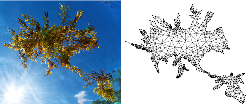
Figure 1: (left) Floating raft of Sargassum. Credit: Alain M. Brin, Blue Glass Photography. (right) Elastic network of finite-size, buoyant particles providing a minimal representation for the raft on the left.

2 The model

To construct the mathematical model, we consider a (possibly irregular) network of $N>1$ spherical particles (beads) connected by (massless, nonbendable) springs. The particles are assumed to have small radius, denoted by $a$, and to be characterized by a water-to-particle density ratio $\delta\geq 1$ finite, so $1-\delta^{-1}$ approximates well (Olascoaga et al., 2020) reserve volume assuming that the air-to-particle density ratio is very small. The elastic force (per unit mass) exerted on particle $i$, with 2-dimensional Cartesian position $x_{i}=(x^{1}_{i},x^{2}_{i})$, by neighboring particles at positions $\{x_{j}:j\in\operatorname{neighbor}(i)\}$, is assumed to obey Hooke’s law (cf. e.g. Goldstein, 1981):

$$F_{i}=-\sum_{j\in\operatorname{neighbor}(i)}k_{ij}\big{(}|x_{ij}|-\ell_{ij}\big{)}\frac{x_{ij}}{|x_{ij}|},$$ (1)

$i=1,\dotsc,N$, where

$$x_{ij}:=x_{i}-x_{j};$$ (2)

$k_{ij}\geq 0$ is the stiffness (per unit mass) of the spring connecting particle $i$ with neighboring particle $j$; and $\ell_{ij}\geq 0$ is the length of the latter at rest. Elastic network models are commonly employed to represent biological macromolecules in the study of dynamics and function of proteins (Bahar et al., 1997). Elastic chain models, a particular form of elastic network models, are used to represent polymers (Bird et al., 1977). A relevant recent application (Picardo et al., 2018) is the investigation of preferential sampling of inertial chains in turbulent flow.

According to the Maxey–Riley theory for inertial ocean motion (Beron-Vera et al., 2019b; Olascoaga et al., 2020), a particle of the elastic network, when taken in isolation, evolves according to the following 2nd-order ordinary differential equation (Appendix A)

$$\ddot{x}+\left(f+\tfrac{1}{3}R\omega\right)\dot{x}^{\perp}+\tau^{-1}\dot{x}=R\frac{\operatorname{D}\!{v}}{\operatorname{D}\!{t}}+R\left(f+\tfrac{1}{3}\omega\right)v^{\perp}+\tau^{-1}u,$$ (3)

where

$$u:=(1-\alpha)v+\alpha v_{\mathrm{a}}$$ (4)

and $\perp$ represents a $+\frac{1}{2}\pi$ rotation. Time-and/or-position-dependent quantities in (3)–(4) are: the (horizontal) velocity of the water, $v$, with $\frac{\operatorname{D}\!{}}{\operatorname{D}\!{t}}v=\partial_{t}v+(\nabla v)v$ where $\nabla$ is the gradient operator in $\mathbb{R}^{2}$; the water’s vorticity, $\omega$; the air velocity, $v_{\mathrm{a}}$; and the Coriolis “parameter,” $f=f_{0}+\beta x^{2}$, where $f_{0}=2\Omega\sin\vartheta_{0}$ and $\beta=2a_{\odot}^{-1}\Omega\cos\vartheta_{0}$ with $\Omega$ and $a_{\odot}$ being Earth’s angular velocity magnitude and mean radius, respectively, and $\vartheta_{0}$ being reference latitude. Quantities independent of position and time in (3)–(4) in turn are:

$$R(\delta):=\frac{1-\frac{1}{2}\Phi(\delta)}{1-\frac{1}{6}\Phi(\delta)}\in[0,1);$$ (5)

$$\tau(\delta):=\frac{1-\frac{1}{6}\Phi(\delta)}{\left(1+(1-\gamma)\Psi(\delta)\right)\delta^{4}}\cdot\frac{a^{2}\rho}{3\mu}>0,$$ (6)

which measures the inertial response time of the medium to the particle ($\rho$ is the assumed constant water density and $\mu$ the water dynamic viscosity); and

$$\alpha(\delta):=\frac{\gamma\Psi(\delta)}{1+(1-\gamma)\Psi(\delta)}\in[0,1),$$ (7)

which makes the convex combination (4) a weighted average of water and air velocities ($\gamma\approx 1/60$ is the air-to-water viscosity ratio). Here

$$\Phi(\delta):=\frac{\mathrm{i}\sqrt{3}}{2}\left(\varphi(\delta)^{-1}-\varphi(\delta)\right)-\frac{1}{2}(\varphi(\delta)^{-1}+\varphi(\delta))+1\in[0,2)$$ (8)

is the fraction of emerged particle piece’s height, where

$$\varphi(\delta):=\sqrt[3]{\mathrm{i}\sqrt{1-(2\delta^{-1}-1)^{2}}+2\delta^{-1}-1}$$ (9)

and

$$\Psi(\delta):=\pi^{-1}\cos^{-1}(1-\Phi(\delta))-\pi^{-1}(1-\Phi(\delta))\smash{\sqrt{1-(1-\Phi(\delta))^{2}}}\in[0,1),$$ (10)

which gives the fraction of emerged particle’s projected (in the flow direction) area. The Sargassum raft drift model is obtained by adding the elastic force (1) to the right-hand-side of the Maxey–Riley set (3). The result is a set of $N$ 2nd-order ordinary differential equations, coupled by the elastic term, viz.,

$$\ddot{x}_{i}+\left(\left.f\right|_{i}+\tfrac{1}{3}R\left.\omega\right|_{i}\right)\dot{x}_{i}^{\perp}+\tau^{-1}\dot{x}_{i}=R\frac{\operatorname{D}\!{\left.v\right|_{i}}}{\operatorname{D}\!{t}}+R\left(\left.f\right|_{i}+\tfrac{1}{3}\left.\omega\right|_{i}\right)\left.v\right|_{i}^{\perp}+\tau^{-1}\left.u\right|_{i}+F_{i},$$ (11)

$i=1,\dotsc,N$, where $\left.\right|_{i}$ means pertaining to particle $i$.

Now, as the radius ($a$) of the elastically interacting particles is small by assumption, the inertial response time ($\tau\propto a^{2}$) is short. We write, then, $\tau=O(\varepsilon)$ where $0<\varepsilon\ll 1$ is a parameter that we use to measure smallness throughout this paper. In this case $\varepsilon$ can be interpreted as a Stokes number (Cartwright et al., 2010). That $\tau=O(\varepsilon)$ has an important consequence: (11) represents a singular perturbation problem involving slow, $x_{i}$, and fast, $v_{i}=\dot{x}_{i}$, variables. This readily follows by rewriting (11) as a system of 1st-order ordinary differential equations in $(x_{i},v_{i})$, i.e. a nonautonomous $4$-dimensional dynamical system, which reveals that while $x_{i}$ changes at $O(1)$ speed, $v_{i}$ does it at $O(\varepsilon^{-1})$ speed. The geometric singular perturbation theory of Fenichel (Fenichel, 1979; Jones, 1995) extended to nonautonomous systems (Haller & Sapsis, 2008) was applied by Beron-Vera et al. (2019b) to (3) to frame its slow manifold, to wit, a $(2+1)$-dimensional subset $\{(x,v_{\mathrm{p}},t):v_{\mathrm{p}}=u(x,t)+u_{\tau}(x,t)+O(\varepsilon^{2})\}$ of the $(4+1)$-dimensional phase space $(x,v_{\mathrm{p}},t)$ where

$$u_{\tau}=\tau\left(R\frac{\operatorname{D}\!{v}}{\operatorname{D}\!{t}}+R\left(f+\tfrac{1}{3}\omega\right)v^{\perp}-\frac{\operatorname{D}\!{u}}{\operatorname{D}\!{t}}-\left(f+\tfrac{1}{3}R\omega\right)u^{\perp}\right)$$ (12)

with $\frac{\operatorname{D}\!{}}{\operatorname{D}\!{t}}u=\partial_{t}u+(\nabla u)u$, which normally attracts all solutions of (3) exponentially in time. On the slow manifold, equation (3) reduces to a 1st-order ordinary differential equation in $x$ given by $\dot{x}=v_{\mathrm{p}}=u+u_{\tau}+O(\varepsilon^{2})$, which represents a nonautonomous $2$-dimensional dynamical system. Mathematically more tractable than the full set (3), this reduced set facilitated uncovering aspects of the inertial ocean dynamics such as the occurrence of great garbage patches in the ocean’s subtropical gyres (Beron-Vera et al., 2016, 2019b) and the potential role of mesoscale eddies (vortices) as flotsam traps (Beron-Vera et al., 2015; Haller et al., 2016; Beron-Vera et al., 2019b). Because the elastic force (1) does not depend on velocity, the geometric singular perturbation analysis of (3) by Beron-Vera et al. (2019b) applies to (11) with the only difference that the equations on the slow manifold are coupled by the elastic force (1), namely,

$$\dot{x}_{i}=v_{i}=\left.u\right|_{i}+\left.u_{\tau}\right|_{i}+\tau F_{i}+O(\varepsilon^{2}),$$ (13)

$i=1,\dotsc,N$. The slow manifold of (11) is the $(2N+1)$-dimensional subset $\{(x_{i},v_{i},t):v_{i}=u(x_{i},t)+u_{\tau}(x_{i},t)+\tau F_{i}(x_{i};x_{j}:j\in\operatorname{neighbor}(i))+O(\varepsilon^{2}),\,i=1,\dotsc,N\}$ of the $(4N+1)$-dimensional phase space $(x_{i},v_{i},t)$, $i=1,\dotsc,N$.

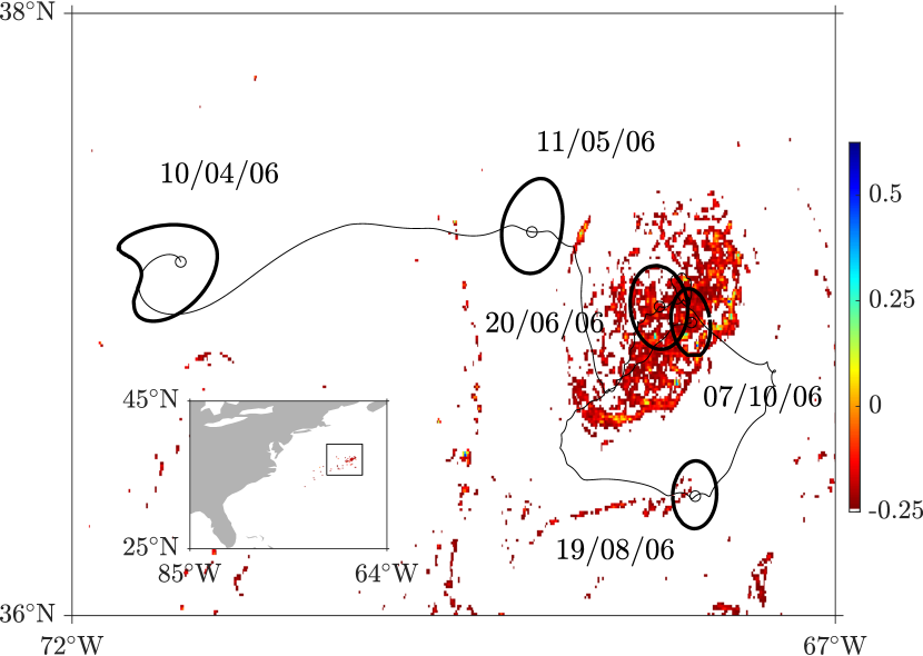
Figure 2: Floating Sargassum distribution inferred from satellite spectrometry on the first week of October 2006 in the region of the Northwestern Atlantic indicated in the inset map. Sargassum corresponds to Maximum Chlorophyll Index (MCI) values exceeding $-0.25$ mW m^-2 sr^-1 nm^-1. MCI is inferred from the Medium Resolution Imaging Spectrometer (MERIS) aboard Envisat. Overlaid in heavy black are snapshots of the evolution of the boundary of a coherent material vortex revealed from satellite altimetry data. The small open circle represents the center of the vortex and the black curve the corresponding trajectory.

3 Behavior near mesoscale eddies

Having settled on a Maxey–Riley equation for Sargassum raft drift, we turn to evaluate its ability to represent reality. This evaluation is not meant to be exhaustive; such type of evaluation is left for a future publication. With this in mind, we consider an actual observation of Sargassum, in the Northwestern Atlantic (Figure 2). This figure more precisely shows, on the first week of October 2006, satellite-derived Maximum Chlorophyll Index (MCI) at the ocean surface. Floating Sargassum corresponds to MCI values exceeding $-0.25$ mW m^-2 sr^-1 nm^-1 (Gower et al., 2008, 2013). Note the spiraled shape of high-MCI distribution filling a compact region. Overlaid on the MCI distribution are snapshots of the evolution of a coherent material vortex/eddy, as extracted from satellite altimetry measurements of sea surface height, widely used to investigate mesoscale (50–200 km) variability in the ocean (Fu et al., 2010). Shown in heavy black is the boundary of the vortex; the (small) open circle and thin black curve indicate its center and trajectory described, respectively. Below we will give precise definitions for all these objects. What is important to be realized at this point is that, being material, the boundary of such a vortex, which can be identified with the core of a cold Gulf Stream ring (vortex) (Talley et al., 2011), cannot be traversed by water. Yet it may be bypassed by inertial particles, whose motion is not tied (Haller & Sapsis, 2008; Beron-Vera et al., 2015) to Lagrangian coherent structures (Haller & Yuan, 2000; Haller, 2016). But this is not enough to explain the collection of Sargassum inside the ring. In fact, this ring is cyclonic (a water particle along the boundary circulates in the local Earth rotation’s sense, which is anticlockwise in the northern hemisphere), and inertial particles tend to collect inside anticyclonic vortices while avoiding cyclonic vortices, as it was formally shown by Beron-Vera et al. (2019b) in agreement with a similar observed tendency of plastic debris in the North Atlantic subtropical gyre (Brach et al., 2018). The relevant question is whether elastic interaction alters this paradigm.

We begin by addressing this question via direct numerical experimentation. This is done by integrating (3) for an elastic network of inertial particles centered at a point on the boundary of the coherent material vortex on 10/04/06. The water velocity $v$ is inferred using altimetry, following standard practice (e.g. Beron-Vera et al., 2008). In turn, the air velocity ($v_{\mathrm{a}}$) is obtained from reanalysis (Dee et al., 2011). While these velocities provide an admittedly imperfect representation of the carrying flow, they are data based and hence enable a comparison with observed behavior. Parameters characterizing the carrying fluid system are set to mean values, namely, $\rho=1025$ kg m^-3, $\rho_{\mathrm{a}}=1.2$ kg m^-3, $\mu=0.001$ kg m^-1s^-1, and $\mu_{\mathrm{a}}=1.8\times 10^{-5}$ kg m^-1s^-1. The initial network is chosen to be a square of 12.5-km side (it could be chosen irregular, if desired, as that one obtained from Delaunay triangulation of polygonal regions spanning the area covered by the Sargassum raft in Figure 7). The network’s springs are of equal length at rest, $\ell_{ij}=0.5$ m. The beads, totalling $n=625$, have a common radius $a=0.1$ m. The buoyancies of the beads are all taken the same and equal to $\delta=1.25$, which has been found appropriate for Sargassum (Olascoaga et al., 2020). The resulting inertial parameters $\alpha=5.9\times 10^{-3}$, $R=0.6$, and $\tau=4.1\times 10^{-2}$ d. Shown in red in Figure 3 are snapshots (on 11/05/06, 20/06/06, and 07/10/06) of the evolution of the network for two different stiffness values, $k_{ij}=4.25$ d^-2 (top) and $k_{ij}=425$ d^-2 (bottom). For reference, inertial particles, unconstrained by elastic forces, i.e. with motion obeying (3) or (11) with $F_{i}=0$, are shown in blue, and the boundary and trajectory of the center of the coherent material vortex are shown in black. The inertial particles, consistent with Beron-Vera et al.’s (2019) prediction, are repelled away from the vortex. By contrast, the elastic network of inertial particles remains close to it when $k_{ij}=4.25$ d^-2 or, much more consistent with the observed Sargassum distribution in Figure 2, collect inside the vortex when $k_{ij}=425$ d^-2. In Figure 4 we show the results of the same numerical experiments when the sense of the planet’s rotation is artificially changed, mimicking conditions in the southern hemisphere. This is achieved by multiplying the Coriolis parameter ($f$) by $-1$. The effect of this alteration first is a change in the polarity of the vortex from cyclonic to anticyclonic. The second, more important effect is that the inertial particles of the network, irrespective of whether they elastically interact or not, are attracted into the vortex. Next we show how analytic treatment of the reduced Maxey–Riley set (13) sheds light on the numerically inferred behavior just described.

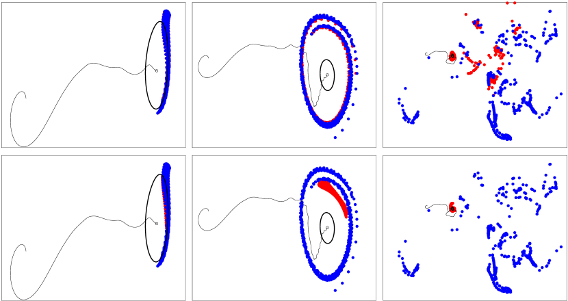
Figure 3: Snapshots of the evolution of elastic networks of inertial particles (red) initially lying on the boundary of the coherent material vortex of Figure 2. From left to right are positions 30, 60, and 180 d after initialization on 10/04/06. The stiffness of the network in the top panels is smaller than that in the bottom panels. Blue dots, shown for reference, correspond to inertial particles which do not interact elastically. Overlaid in all panels are the boundary of the vortex (heavy black), center (small open circle), and corresponding trajectory (black curve).

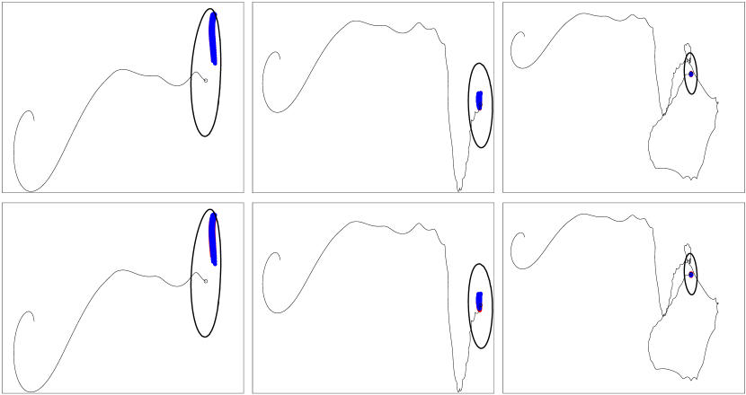
Figure 4: As in Fig. 3, but with the sign of Coriolis parameter ($f$) artificially set negative.

4 A formal result

With the above goal in mind, we first make the coherent material vortex notion precise. This is done by considering the Lagrangian-averaged vorticity deviation or LAVD field: Haller et al. (2016)

$$\operatorname{LAVD}_{t_{0}}^{t}(x_{0}):=\int_{t_{0}}^{t}|\omega(F_{t_{0}}^{t^{\prime}}(x_{0}),t^{\prime}),t^{\prime})-\bar{\omega}(t^{\prime})|\operatorname{d}\!{t^{\prime}},$$ (14)

where

$$\bar{\omega}(t)=\frac{1}{\operatorname{area}U(t)}\int_{U(t)}\omega(x,t)\,\mathrm{d}^{2}x,$$ (15)

which is an average of the vorticity over a region of water $U(t)=F_{t_{0}}^{t}U(t_{0})$. Here $F_{t_{0}}^{t}$ is the flow map that takes water particle positions $x_{0}$ at time $t_{0}$ to positions $x$ at time $t$. As defined by Haller et al. (2016), a rotationally coherent vortex over $t\in[t_{0},t_{0}+T]$ is an evolving material (water) region $V(t)\subset U(t)$, $t\in[t_{0},t_{0}+T]$, such that its time-$t_{0}$ position is enclosed by the outermost, sufficiently convex isoline of $\operatorname{LAVD}_{t_{0}}^{t_{0}+T}(x_{0})$ around a local (nondegenerate) maximum (resp., minimum) is $T>0$ (resp., $T<0$). (To be more precise, a region $V(t)$ may contain several local extrema (Beron-Vera et al., 2019a), but we conveniently exclude from consideration such situations here to enable a straightforward definition of vortex center (Haller et al., 2016).) As a consequence, the elements of the boundaries of such material regions $V(t)$ complete the same total material rotation relative to the mean material rotation of the whole water mass in the domain $U(t)$ that contains them. This property of the boundaries tends (Haller et al., 2016) to restrict their filamentation to be mainly tangential under advection from $t_{0}$ to $t_{0}+T$. Furthermore, the ensuing water-holding-property of rotationally coherent eddies and related elliptic Lagrangian coherent structures (Haller & Beron-Vera, 2013, 2014; Farazmand & Haller, 2016; Haller et al., 2018), verified numerically extensively (Haller et al., 2016; Beron-Vera et al., 2019a) and observed in controlled laboratory experiments (Tel et al., 2018, 2020) and field surveys involving in-situ (buoy trajectories) and remote (satellite-inferred chlorophyll distributions) measurements (Beron-Vera et al., 2018), can be so enduring (Wang et al., 2015, 2016) for the water-holding-property to provide a very effective long-range transport mechanism in the ocean consistent with traditional oceanographic expectation (Gordon, 1986). The material vortex in Figure 2 (and also 3 and 4) is of the rotationally coherent class just described. It was obtained by applying LAVD analysis on $t_{0}=$ 07/10/06, a day of the week when the Sargassum raft observation in Figure 2 was acquired, using $T=-180$ d. This turned out to be the longest backward-time integration from which a closed LAVD isoline with a stringent convexity deficiency of $10^{-3}$ was possible to find. It represents a rather long backward-time integration, which dates the “genesis” of the rotationally coherent vortex around $t_{0}+T=$ 10/04/06. Figure 2 not only shows the vortex boundary on detection date ($t_{0}$), but also several advected images of it under the backward-time flow out to $t_{0}+T$.

The second step in reaching the goal above is to assume that set (13), which attracts all solutions of (11), can be approximated by

$$\dot{x}_{i}=v_{i}=gf_{0}^{-1}\nabla^{\perp}\left.\eta\right|_{i}+\tau\big{(}g(1-\alpha-R)\nabla\left.\eta\right|_{i}+F_{i}\big{)}$$ (16)

$+\,O(\varepsilon^{2})$, $i=1,\dotsc,N$, which is justified as follows. First, the near surface ocean flow is in quasigeostrophic balance (Pedlosky, 1987), as it can be expected for mesoscale ocean flow (Fu et al., 2010). Interpreting $\varepsilon$ as a Rossby number (Pedlosky, 1987), this means that $v=gf_{0}^{-1}\nabla^{\perp}\eta+O(\varepsilon^{2})$, where $g$ is gravity and $\eta=O(\varepsilon)$ sea surface height, $\partial_{t}=O(\varepsilon)$, and $f=f_{0}+O(\varepsilon)$. Second, the elastic interaction does not alter the nature of the critical and slow manifolds, which is guaranteed by making $F_{i}=O(\varepsilon)$. Third, $\alpha=O(\varepsilon)$, at least, consistent with it being very small (a few percent) over a large range of buoyancy ($\delta$) values; cf. Figure 2 of Beron-Vera et al. (2019b). Indeed, taking $\delta=1.25$ (as it was found appropriate by Olascoaga et al. (2020) for Sargassum), recall we estimated $\alpha\approx 5\times 10^{-3}$. This is actually quite small, and more consistent with $\alpha=O(\varepsilon^{3})$ for a Rossby number that typically characterizes mesoscale flow ($\varepsilon=0.1$). Note that this makes $\alpha v_{\mathrm{a}}=O(\varepsilon^{3})$ for an $O(1)$ near surface atmospheric flow. But this would not be consistent with the quasigeostrophic ocean flow assumption. So we require, fourth, that $v_{\mathrm{a}}=O(\varepsilon^{2})$, at least, i.e. the wind field over the period of interest is sufficiently weak (calm).

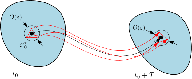
Figure 5: By smooth dependence of the solutions of (16) on parameters, an elastic network of inertial particles initially $O(\varepsilon)$-close to the center of $x_{0}^{*}$ of a rotationally coherent vortex will remain $O(\varepsilon)$-close to the trajectory flowing from it over a finite-time interval $[t_{0},t_{0}+T]$.

Now, let $\mathbf{x}:=(x_{1}^{1},\dotsc,x_{N}^{1},x_{1}^{2},\dotsc,x_{N}^{2})$ and $\mathbf{v}:=(v_{1}^{1},\dotsc,v_{N}^{1},v_{1}^{2},\dotsc,v_{N}^{2})$. Then write (16) as

$$\dot{\mathbf{x}}=\mathbf{v}(\mathbf{x},t)$$ (17)

We denote $\mathbf{F}_{t_{0}}^{t}$ the corresponding flow map, namely, $\mathbf{F}_{t_{0}}^{t}(\mathbf{x}_{0}):=\mathbf{x}(t;\mathbf{x}_{0},t_{0})$ where $\mathbf{x}_{0}=\mathbf{x}(t_{0})$. Following Haller et al. (2016) closely, we invoke Liouville’s theorem (e.g. Arnold, 1989) and note that a trajectory $\smash{\mathbf{F}_{t_{0}}^{t}}(\mathbf{x}_{0})$ is overall forward attracting over $t\in[t_{0},t_{0}+T]$, $T>0$ (resp., $T<0$), if $\det\smash{\operatorname{\mathbf{D}}\!{\mathbf{F}}_{t_{0}}^{t_{0}+T}}(\mathbf{x}_{0})<1$ (resp., $\det\smash{\operatorname{\mathbf{D}}\!{\mathbf{F}}_{t_{0}}^{t_{0}+T}}(\mathbf{x}_{0})>1$). Let us suppose now that the time-$t_{0}$ position of the network of elastically connected inertial particles is very close to the center of a rotationally coherent vortex, given by (Haller et al., 2016)

$$x_{0}^{*}=\operatorname*{arg\,max}_{x_{0}\in V(t_{0})}\operatorname{LAVD}_{t_{0}}^{t_{0}+T}(x_{0}),$$ (18)

which is expected to exist in a well-defined fashion when the ocean flow is quasigeostrophic, as we have assumed here. We write the above formally as $|x_{i}(t_{0})-x_{0}^{*}|=O(\varepsilon)$, $i=1,\dotsc,N$. Then, by smooth dependence of the solutions of (16) on parameters, for $t\in[t_{0},t_{0}+T]$ finite, one has

$$x_{i}(t;x_{i}(t_{0}),t_{0})=F_{t_{0}}^{t}(x_{0}^{*})+O(\varepsilon),$$ (19)

$i=1,\dotsc,N$, where $F_{t_{0}}^{t}$ is the flow map generated by the quasigeostrophic ocean velocity field $gf_{0}^{-1}\nabla^{\perp}\eta$ (Figure 5). With this in mind, we find (Appendix B)

$$\det\operatorname{\mathbf{D}}\!{\mathbf{F}}_{t_{0}}^{t_{0}+T}(\mathbf{x}_{0})=\exp\tau(\mathcal{A}+\mathcal{B})$$ (20)

$+\,O(\varepsilon^{2})$, where

$$\mathcal{A}:=gN(1-\alpha-R)\mathop{\rm sign}_{t\in[t_{0},t_{0}+T]}\big{(}T\nabla^{2}\eta(F_{t_{0}}^{t}(x_{0}^{*}),t)\big{)}\cdot\left|\int_{t_{0}}^{t_{0}+T}|\nabla^{2}\eta(F_{t_{0}}^{t}(x_{0}^{*}),t)|\operatorname{d}\!{t}\right|$$ (21)

and

$$\mathcal{B}:=-T\sum_{i=1}^{N}\sum_{j\in\operatorname{neighbor}(i)}k_{ij}.$$ (22)

Noting that $1-\alpha-R\geq 0$, it finally follows that:

Theorem 1

$F_{t_{0}}^{t}(x_{0}^{*})$ is locally forward attracting overall over $t\in[t_{0},t_{0}+T]$:

1. for all $k_{ij}$ when $\mathop{\rm sign}_{t\in[t_{0},t_{0}+T]}\nabla^{2}\eta(F_{t_{0}}^{t}(x_{0}^{*}),t)<0$; and

2. provided that

   $$|T|\sum_{i=1}^{N}\sum_{j\in\operatorname{neighbor}(i)}k_{ij}>gN(1-\alpha-R)\left|\int_{t_{0}}^{t_{0}+T}|\nabla^{2}\eta(F_{t_{0}}^{t}(x_{0}^{*}),t)|\operatorname{d}\!{t}\right|$$ (23)

   when $\mathop{\rm sign}_{t\in[t_{0},t_{0}+T]}\nabla^{2}\eta(F_{t_{0}}^{t}(x_{0}^{*}),t)>0$.

Since $\omega=gf_{0}^{-1}\nabla^{2}\eta+O(\varepsilon^{2})$, the above result says that the center of a cyclonic rotationally coherent quasigeostrophic eddy represents a finite-time attractor for elastic networks of inertial particles in the presence of calm winds if they are sufficiently stiff, while that of an anticyclonic eddy irrespective of how stiff. The minimal stiffness $k_{\min}$ required for a cyclonic eddy center to attract an elastic inertial network over finite time decreases with network’s size. This can be readily seen assuming that the stiffness is the same for all pairs of elastically connected particles, say, $k_{ij}=k$, and considering a square network with $N=n^{2}$ elements. In such a case one easily computes $\smash{\sum_{i=1}^{N}\sum_{j\in\operatorname{neighbor}(i)}}=4n(n-1)$ and thus $k_{\min}=\smash{\frac{n}{4(n-1)}}(1-\alpha-R)|f_{0}T^{-1}\operatorname{LAVD}_{t_{0}}^{t_{0}+T}(x_{0}^{*})|+O(\varepsilon^{2})$, which decays to a value bounded away from 0 as $n\to\infty$. (In getting the last result we have relied on the fact that $U(t)$ in (15) can be taken as large as desired, e.g. $\operatorname{area}U(t)=O(\varepsilon^{-1})$ as we have specifically set.) So as the size of the network increases, the condition on the stiffness is expected to be more easily satisfied. Similarly, this condition is easier to be fulfilled as the buoyancy of the particles approaches neutrality; indeed, $\lim_{\delta\to 1}k_{\min}=0$. Note, on the other hand, that $\lim_{n\to 1}k_{\min}=\infty$. Thus, as expected, the result of Beron-Vera et al. (2019b) for isolated inertial particles is recovered: while anticyclonic eddy centers attract finite-size particles floating at the ocean surface, cyclonic ones always repel them away. It is important to realize that statements on the existence of finite-time attractors inside rotationally coherent eddies do not say anything about basins of attraction. Yet the expectation, verified numerically above in qualitative agreement with remote-sensing data, is that mesoscale eddies will in general trap Sargassum rafts if they initially lie near their boundaries (the sensitivity analysis in Appendix C provides further numerical support for this expectation).

5 Concluding remarks

The above formal result provides an explanation for the behavior of the elastic network in Figures 3 and 4. This encourages us to speculate that Sargassum rafts should behave similarly. Of course, there are additional (physical) processes in the ocean that may also play a role. For instance, downwelling associated with submesoscale (less than 10 km) motions can lead to surface convergence of flotsam. While such convergence has been recently observed (D’Asaro et al., 2018), numerical simulations and theoretical arguments (McWilliams, 2016) suggest that this should happen at the periphery of submesoscale cyclonic vortices, where density contrast is large. Yet, consistent with this work, initial inspection of satellite images is revealing (Triñanes, 2020) that Sargassum collection is not restricted to vortex peripheries and further that both cyclonic and anticyclonic eddies trap Sargassum.

We note too that pelagic Sargassum is reportedly (Sheinbaum, 2020) observed to sometimes be found beneath the sea surface, which can be a result of downwellings and/or reductions of the buoyancy of the rafts as they absorb water or undergo physiological transformations. The effects of the latter can be incorporated into the minimal model of this paper, partially at least, by making $\delta\geq 1$ a function of time, as it has been done previously (Tanga & Provenzale, 1994) in the standard Maxey–Riley set. Full representation, beyond the scope at present, of possible three-dimensional aspects of the motion of Sargassum rafts will require one to consider the (vertical) buoyancy force along with a reliable representation of the three components of the ocean velocity field, coupled with an ecological model of Sargassum life cycle.

We close by noting that satellite-altimetry observations reveal a dominant tendency of mesoscale eddies of either polarity to propagate westward (Morrow et al., 2004; Chelton et al., 2011) consistent with theoretical argumentation (Nof, 1981; Cushman-Roisin et al., 1990; Graef, 1998; Ripa, 2000). This observational evidence, along with the additional observational evidence on the long-range transport capacity of eddies (Wang et al., 2015, 2016; Beron-Vera et al., 2018), makes the result of this paper a potentially very effective mechanism for the connectivity of Sargassum between the Caribbean Sea and remote regions in the tropical North Atlantic. Clearly, a comprehensive modeling effort is needed to verify this hypothesis. The are several parameters that will require specification, which may be obtained from a study of the architecture of Sargassum rafts or, alternatively, from observed evolution (as inferred from satellite imagery) via regression or learning (e.g. Aksamit et al., 2020).

Appendix A Review of the Maxey–Riley set (3)

The exact motion of inertial particles obeys the Navier–Stokes equation with moving boundaries as such particles are extended objects in the fluid with their own boundaries. This results in complicated partial differential equations which are hard to solve and analyze. Here, as well as in Beron-Vera et al. (2019b), the interest is in the approximation, formulated in terms of an ordinary differential equation, provided by the Maxey–Riley equation (Maxey & Riley, 1983), the de-jure fluid mechanics paradigm for inertial particle dynamics.

Such an equation is a classical mechanics Newton’s second law with several forcing terms that describe the motion of solid spherical particles immersed in the unsteady nonuniform flow of a homogeneous viscous fluid. Normalized by particle mass, $m_{\mathrm{p}}=\frac{4}{3}\pi a^{3}\rho_{\mathrm{p}}$, the relevant forcing terms for the horizontal motion of a sufficiently small particle, excluding so-called Faxen corrections and the Basset-Boussinesq history or memory term, are: 1) the flow force exerted on the particle by the undisturbed fluid,

$$F_{\mathrm{flow}}=\frac{m_{\mathrm{f}}}{m_{\mathrm{p}}}\frac{\operatorname{D}\!{v_{\mathrm{f}}}}{\operatorname{D}\!{t}},$$ (24)

where $m_{\mathrm{f}}=\frac{4}{3}\pi a^{3}\rho_{\mathrm{f}}$ is the mass of the displaced fluid (of density $\rho_{\mathrm{f}}$), and $\smash{\frac{\operatorname{D}\!{v_{\mathrm{f}}}}{\operatorname{D}\!{t}}}$ is the material derivative of the fluid velocity ($v_{\mathrm{f}}$) or its total derivative taken along the trajectory of a fluid particle, $x=X_{\mathrm{f}}(t)$, i.e., $\smash{\frac{\operatorname{D}\!{v_{\mathrm{f}}}}{\operatorname{D}\!{t}}}=\smash{\left[\frac{\operatorname{d}\!{}}{\operatorname{d}\!{t}}v_{\mathrm{f}}(x,t)\right]_{x=X_{\mathrm{f}}(t)}}=\partial_{t}v_{\mathrm{f}}+(\nabla v_{\mathrm{f}})v_{\mathrm{f}}$; 3) the added mass force resulting from part of the fluid moving with the particle,

$$F_{\mathrm{mass}}=\frac{\frac{1}{2}m_{\mathrm{f}}}{m_{\mathrm{p}}}\left(\frac{\operatorname{D}\!{v_{\mathrm{f}}}}{\operatorname{D}\!{t}}-\dot{v}_{\mathrm{p}}\right),$$ (25)

where $\dot{v}_{\mathrm{p}}$ is the acceleration of an inertial particle with trajectory $x=X_{\mathrm{p}}(t)$, i.e., $\dot{v}_{\mathrm{p}}=\smash{\frac{\operatorname{d}\!{}}{\operatorname{d}\!{t}}\left[v_{\mathrm{p}}(x,t)\right]_{x=X_{\mathrm{p}}(t)}}=\partial_{t}v_{\mathrm{p}}$ where $v_{\mathrm{p}}=\partial_{t}X_{\mathrm{p}}=\dot{x}$ is the inertial particle velocity; 2) the lift force, which arises when the particle rotates as it moves in a (horizontally) sheared flow,

$$F_{\mathrm{lift}}=\frac{\frac{1}{2}m_{\mathrm{f}}}{m_{\mathrm{p}}}\omega_{\mathrm{f}}(v_{\mathrm{f}}-v_{\mathrm{p}})^{\perp},$$ (26)

where $\omega_{\mathrm{f}}=\partial_{1}v^{2}_{\mathrm{f}}-\partial_{2}v^{1}_{\mathrm{f}}$ is the (vertical) vorticity of the fluid; and 4) the drag force caused by the fluid viscosity,

$$F_{\mathrm{drag}}=\frac{12\mu_{\mathrm{f}}\frac{A_{\mathrm{f}}}{\ell_{\mathrm{f}}}}{m_{\mathrm{p}}}(v_{\mathrm{f}}-v_{\mathrm{p}}),$$ (27)

where $\mu_{\mathrm{f}}$ is the dynamic viscosity of the fluid, and $A_{\mathrm{f}}$ ($=\pi a^{2}$) is the projected area of the particle and $\ell_{\mathrm{f}}$ ($=2a$) is the characteristic projected length, which we have intentionally left unspecified for future appropriate evaluation.

The above forces are included in the original formulation by Maxey & Riley (1983), except for the lift force (26), due to Auton (1987) and a form of the added mass term different than (25), which corresponds to the correction due to Auton et al. (1988). The specific form of lift force (26) can be found in Montabone (2002, Chapter 4) (cf. similar forms in Henderson et al., 2007; Sapsis et al., 2011).

To derive equation (3), Beron-Vera et al. (2019b) first accounted for the geophysical nature of the fluid by including the Coriolis force. (In an earlier geophysical adaptation of the Maxey–Riley equation (Provenzale, 1999), the centrifugal force was included as well, but this is actually balanced out by the gravitational force on the horizontal plane.) This amounts to replacing (24) and (25) with

$$F_{\mathrm{flow}}=\frac{m_{\mathrm{f}}}{m_{\mathrm{p}}}\left(\frac{\operatorname{D}\!{v_{\mathrm{f}}}}{\operatorname{D}\!{t}}+fv_{\mathrm{f}}^{\bot}\right)$$ (28)

and

$$F_{\mathrm{mass}}=\frac{\frac{1}{2}m_{\mathrm{f}}}{m_{\mathrm{p}}}\left(\frac{\operatorname{D}\!{v_{\mathrm{f}}}}{\operatorname{D}\!{t}}+fv_{\mathrm{f}}^{\bot}-\dot{v}_{\mathrm{p}}-fv_{\mathrm{p}}^{\bot}\right),$$ (29)

respectively.

Then, noting that fluid variables and parameters take different values when pertaining to seawater or air, e.g.

$$v_{\mathrm{f}}(x,z,t)=\begin{cases}v_{\mathrm{a}}(x,t)&\text{if }z\in(0,h_{\mathrm{a}}],\\ v(x,t)&\text{if }z\in[-h,0),\end{cases}$$ (30)

Beron-Vera et al. (2019b) wrote

$$\dot{v}_{\mathrm{p}}+fv_{\mathrm{p}}^{\perp}=\langle F_{\mathrm{flow}}\rangle+\langle F_{\mathrm{mass}}\rangle+\langle F_{\mathrm{lift}}\rangle+\langle F_{\mathrm{drag}}\rangle,$$ (31)

where $\langle\,\rangle$ is an average over $z\in[-h,h_{\mathrm{a}}]$. After some algebraic manipulation, equation (3) follows upon making $\ell=\ell_{\mathrm{a}}=\delta^{-3}h$ as suggested by observations (Olascoaga et al., 2020), and assuming $\delta_{\mathrm{a}}\ll 1$ with the static stability considerations in §IV.B of Olascoaga et al. (2020) in mind.

Appendix B Derivation of equations (20)–(22)

We begin by decomposing the elastic force as $F_{i}=A_{i}+B_{i}$, where

$$A_{i}:=-\sum_{j\in\operatorname{neighbor}(i)}k_{ij}x_{ij},\quad B_{i}:=\sum_{j\in\operatorname{neighbor}(i)}k_{ij}\ell_{ij}\frac{x_{ij}}{|x_{ij}|}.$$ (32)

Then we note

$$\nabla_{i}A_{i}=-\sum_{j\in\operatorname{neighbor}(i)}k_{ij}\nabla_{i}x_{ij}=-\sum_{j\in\operatorname{neighbor}(i)}k_{ij}\operatorname{Id}^{2\times 2}$$ (33)

and thus

$$\sum_{i=1}^{N}\operatorname*{trace}\nabla_{i}A_{i}=-\sum_{i=1}^{N}\sum_{j\in\operatorname{neighbor}(i)}k_{ij}\operatorname*{trace}\operatorname{Id}^{2\times 2}=-2\sum_{i=1}^{N}\sum_{j\in\operatorname{neighbor}(i)}k_{ij}.$$ (34)

Now, let $x,y\in\mathbb{R}^{2}$ and note

$$\nabla_{x}\frac{x-y}{|x-y|} =\frac{\nabla_{x}x}{|x-y|}-\frac{(x-y)2(x-y)^{\top}\nabla_{x}x}{2|x-y|^{3}}$$

$$=\frac{\operatorname{Id}^{2\times 2}}{|x-y|}-\frac{(x-y)(x-y)^{\top}\operatorname{Id}^{2\times 2}}{|x-y|^{3}}$$

$$=\frac{\operatorname{Id}^{2\times 2}}{|x-y|}-\frac{(x-y)(x-y)^{\top}}{|x-y|^{3}}.$$ (35)

Consequently,

$$\operatorname*{trace}\nabla_{x}\frac{x-y}{|x-y|} =\operatorname*{trace}\begin{pmatrix}\frac{1}{|x-y|}&0\\ 0&\frac{1}{|x-y|}\end{pmatrix}-\operatorname*{trace}\begin{pmatrix}\frac{(x_{1}-y_{1})^{2}}{|x-y|^{3}}&\frac{(x_{1}-y_{1})(x_{2}-y_{2})}{|x-y|^{3}}\\ \frac{(x_{2}-y_{2})(x_{1}-y_{1})}{|x-y|^{3}}&\frac{(x_{2}-y_{2})^{2}}{|x-y|^{3}}\end{pmatrix}$$

$$=\frac{2}{|x-y|}-\frac{|x-y|^{2}}{|x-y|^{3}}$$

$$=\frac{1}{|x-y|}.$$ (36)

Using (35) we obtain

$$\nabla_{i}B_{i} =-\sum_{j\in\operatorname{neighbor}(i)}k_{ij}\ell_{ij}\left(-\frac{\nabla_{i}x_{ij}}{|x_{ij}|}+\frac{x_{ij}x_{ij}^{\top}}{|x_{ij}|^{3}}\right)$$

$$=-\sum_{j\in\operatorname{neighbor}(i)}k_{ij}\ell_{ij}\left(-\frac{\operatorname{Id}^{2\times 2}}{|x_{ij}|}+\frac{x_{ij}x_{ij}^{\top}}{|x_{ij}|^{3}}\right),$$

while using (36),

$$\sum_{i=1}^{N}\operatorname*{trace}\nabla_{i}B_{i} =-\sum_{i=1}^{N}\sum_{j\in\operatorname{neighbor}(i)}k_{ij}\ell_{ij}\operatorname*{trace}\left(-\frac{\operatorname{Id}^{2\times 2}}{|x_{ij}|}+\frac{x_{ij}x_{ij}^{\top}}{|x_{ij}|^{3}}\right)$$

$$=-\sum_{i=1}^{N}\sum_{j\in\operatorname{neighbor}(i)}k_{ij}\ell_{ij}\left(-\frac{2}{|x_{ij}|}+\frac{1}{|x_{ij}|}\right)$$

$$=\sum_{i=1}^{N}\sum_{j\in\operatorname{neighbor}(i)}k_{ij}\frac{\ell_{ij}}{|x_{ij}|}.$$ (37)

Combining (34) and (37) we obtain

$$\sum_{i=1}^{N}\operatorname*{trace}\nabla_{i}F_{i}=\sum_{i=1}^{N}\sum_{j\in\operatorname{neighbor}(i)}k_{ij}\left(\frac{\ell_{ij}}{|x_{ij}|}-2\right).$$ (38)

Now, taking into account (38), from (16) it follows that

$$\operatorname*{trace}\boldsymbol{\nabla}\mathbf{v}(\mathbf{F}_{t_{0}}^{t}(\mathbf{x}_{0}),t)={} \sum_{1}^{N}\operatorname*{trace}\nabla_{i}v_{i}(x_{i}(t;x_{i}(t_{0}),t_{0}),t)$$

$$={} \tau R_{\alpha}g\sum_{1}^{N}\nabla^{2}\eta(x_{i}(t;x_{i}(t_{0}),t_{0}),t)$$

$$+\tau\sum_{i=1}^{N}\sum_{j\in\operatorname{neighbor}(i)}k_{ij}\left(\frac{\ell_{ij}}{|x_{ij}(t;x_{ij}(t_{0}),t_{0})|}-2\right)+O(\varepsilon^{2})$$

$$={} \tau R_{\alpha}gN\nabla^{2}\eta(F_{t_{0}}^{t}(x_{0}^{*}),t)-\tau\sum_{i=1}^{N}\sum_{j\in\operatorname{neighbor}(i)}k_{ij}+O(\varepsilon^{2}),$$ (39)

where $R_{\alpha}:=1-\alpha-R$. Here we have had (19) in mind, and consistent with this have assumed $\ell_{ij}=O(\varepsilon)$, so $\ell_{ij}/|x_{ij}|\sim 1$ as $\varepsilon\to 0$. Result (20)–(22) follows upon noting that $\det\operatorname{\mathbf{D}}\!{\mathbf{F}}_{t_{0}}^{t}(\mathbf{x}_{0})=\int_{t_{0}}^{t}\operatorname*{trace}\boldsymbol{\nabla}\mathbf{v}(\mathbf{F}_{t_{0}}^{t^{\prime}}(\mathbf{x}_{0}),t^{\prime})\operatorname{d}\!{t^{\prime}}$, where $\boldsymbol{\nabla}$ is the gradient operator in $\mathbb{R}^{2N}$. $\square$

Appendix C Sensitivity analysis

We provide further numerical support for the expectation that mesoscales eddies should in general trap Sargassum rafts through a sensitivity analysis with respect to the elastic network’s initial position relative to the vortex and also the configuration of the initial network. This is given in Figure 6, which uses the same parameters as in bottom panels of Figure 3 except that initialization is made 25 (top) and 50 (bottom) km away from the boundary of the vortex. These distances correspond to about one and two times the mean radius of the vortex, respectively. The initial network’s shape is irregular, obtained by applying a small random perturbation on the original square network’s bead locations (Figure 7). Note the influence of the vortex on the network.

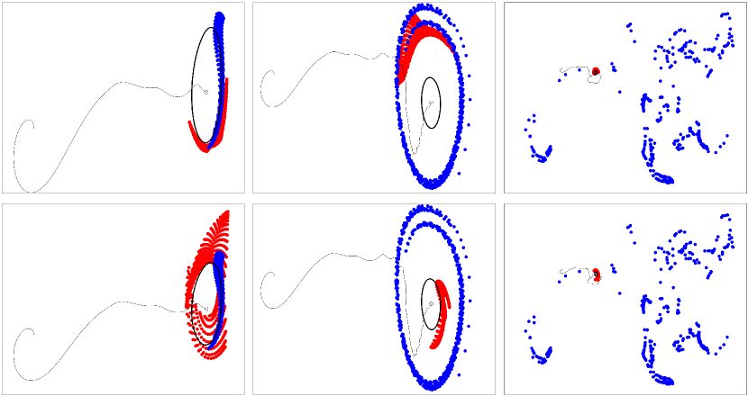
Figure 6: As in the bottom panel of Figure 3, except that the initialization of the elastic networks takes place away from the boundary of the vortex, at a distance equal to one (top) and two times as large as (bottom) the mean radius of the vortex (about 25 km) where the initial network’s bead locations are a small random perturbation of the original locations forming a rectangular grid.

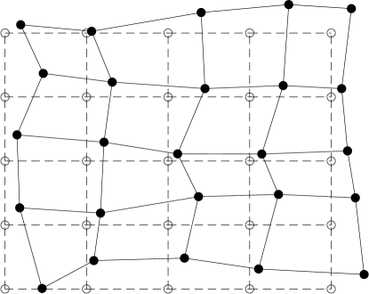
Figure 7: Portions (of about 2.5-km side) of the initial square network employed in Figures 3–4 (beads depicted open) and the irregular network used in Figure 6 (beads depicted solid).

References

- Aksamit et al. (2020) Aksamit, N., Sapsis, T. & Haller, G. 2020 Machine-learning mesoscale and submesoscale surface dynamics from Lagrangian ocean drifter trajectories. J. Phys. Oceanogr. 50, 1179–1196.
- Arnold (1989) Arnold, V. I. 1989 Mathematical Methods of Classical Mechanics, 2nd edn. Springer.
- Auton (1987) Auton, T. R. 1987 The lift force on a spherical body in a rotational flow. Journal of Fluid Mechanics 183, 199–218.
- Auton et al. (1988) Auton, T. R., Hunt, F. C. R. & Prud’homme, M. 1988 The force exerted on a body in inviscid unsteady non-uniform rotational flow. J. Fluid. Mech. 197, 241.
- Babiano et al. (2000) Babiano, A., Cartwright, J. H., Piro, O. & Provenzale, A. 2000 Dynamics of a small neutrally buoyant sphere in a fluid and targeting in Hamiltonian systems. Phys. Rev. Lett. 84, 5,764–5,767.
- Bahar et al. (1997) Bahar, Ivet, Atilgan, Ali Rana & Erman, Burak 1997 Direct evaluation of thermal fluctuations in proteins using a single-parameter harmonic potential. Folding and Design 2 (3), 173 – 181.
- Beron-Vera et al. (2019a) Beron-Vera, F. J., Hadjighasem, A., Xia, Q., Olascoaga, M. J. & Haller, G. 2019a Coherent Lagrangian swirls among submesoscale motions. Proc. Natl. Acad. Sci. U.S.A. 116, 18251–18256.
- Beron-Vera et al. (2018) Beron-Vera, F. J., Olascaoaga, M. J., Wang, Y., nanes, J. Tri & Pérez-Brunius, P. 2018 Enduring Lagrangian coherence of a Loop Current ring assessed using independent observations. Scientific Reports 8, 11275.
- Beron-Vera et al. (2008) Beron-Vera, F. J., Olascoaga, M. J. & Goni, G. J. 2008 Oceanic mesoscale vortices as revealed by Lagrangian coherent structures. Geophys. Res. Lett. 35, L12603.
- Beron-Vera et al. (2015) Beron-Vera, F. J., Olascoaga, M. J., Haller, G., Farazmand, M., Triñanes, J. & Wang, Y. 2015 Dissipative inertial transport patterns near coherent Lagrangian eddies in the ocean. Chaos 25, 087412.
- Beron-Vera et al. (2016) Beron-Vera, F. J., Olascoaga, M. J. & Lumpkin, R. 2016 Inertia-induced accumulation of flotsam in the subtropical gyres. Geophys. Res. Lett. 43, 12228–12233.
- Beron-Vera et al. (2019b) Beron-Vera, F. J., Olascoaga, M. J. & Miron, P. 2019b Building a Maxey–Riley framework for surface ocean inertial particle dynamics. Phys. Fluids 31, 096602.
- Bird et al. (1977) Bird, R. B., Curtiss, C. F., Armstrong, R. C. & Hassager, O. 1977 Dynamics of Polymeric Liquids, , vol. 2. New York: John Wiley and Sons.
- Brach et al. (2018) Brach, Laurent, Deixonne, Patrick, Bernard, Marie-France, Durand, Edmée, Desjean, Marie-Christine, Perez, Emile, van Sebille, Erik & ter Halle, Alexandra 2018 Anticyclonic eddies increase accumulation of microplastic in the north atlantic subtropical gyre. Marine Pollution Bulletin 126, 191–196.
- Cartwright et al. (2010) Cartwright, J. H. E., Feudel, U., Károlyi, G., de Moura, A., Piro, O. & Tél, T. 2010 Dynamics of finite-size particles in chaotic fluid flows. In Nonlinear Dynamics and Chaos: Advances and Perspectives (ed. M. Thiel et al.), pp. 51–87. Springer-Verlag Berlin Heidelberg.
- Chelton et al. (2011) Chelton, D. B., Schlax, M. G. & Samelson, R. M. 2011 Global observations of nonlinear mesoscale eddies. Prog. Oceanogr. 91, 167–216.
- Cushman-Roisin et al. (1990) Cushman-Roisin, B., Chassignet, E. P. & Tang, B. 1990 Westward motion of mesoscale eddies. J. Phys. Oceanogr. 20, 758–768.
- D’Asaro et al. (2018) D’Asaro, Eric A., Shcherbina, Andrey Y., Klymak, Jody M., Molemaker, Jeroen, Novelli, Guillaume, Guigand, Cédric M., Haza, Angelique C., Haus, Brian K., Ryan, Edward H., Jacobs, Gregg A., Huntley, Helga S., Laxague, Nathan J. M., Chen, Shuyi, Judt, Falko, McWilliams, James C., Barkan, Roy, Kirwan, A. D., Poje, Andrew C. & Özgökmen, Tamay M. 2018 Ocean convergence and the dispersion of flotsam. Proceedings of the National Academy of Sciences 115, 1162–1167.
- Dee et al. (2011) Dee, D. P., Uppala, S. M., Simmons, A. J., Berrisford, P., Poli, P., Kobayashi, S., Andrae, U., Balmaseda, M. A., Balsamo, G., Bauer, P., Bechtold, P., Beljaars, A. C. M., van de Berg, L., Bidlot, J., Bormann, N., Delsol, C., Dragani, R., Fuentes, M., Geer, A. J., Haimberger, L., Healy, S. B., Hersbach, H., Holm, E. V., Isaksen, L., Kallberg, P., Kohler, M., Matricardi, M., McNally, A. P., Monge-Sanz, B. M., Morcrette, J.-J., Park, B.-K., Peubey, C., de Rosnay, P., Tavolato, C., Thepaut, J.-N. & Vitart, F. 2011 The ERA-Interim reanalysis: configuration and performance of the data assimilation system. Quart. J. Roy. Met. Soc. 137, 553–597.
- Farazmand & Haller (2016) Farazmand, Mohammad & Haller, George 2016 Polar rotation angle identifies elliptic islands in unsteady dynamical systems. Physica D: Nonlinear Phenomena 315, 1 – 12.
- Fenichel (1979) Fenichel, N. 1979 Geometric singular perturbation theory for ordinary differential equations. J. Differential Equations 31, 51–98.
- Fu et al. (2010) Fu, L. L, Chelton, D. B., Le Traon, P.-Y. & Morrow, R. 2010 Eddy dynamics from satellite altimetry. Oceanography 23, 14–25.
- Goldstein (1981) Goldstein, H. 1981 Classical Mechanics. Addison-Wesley, 672.
- Gordon (1986) Gordon, A. 1986 Interocean exchange of thermocline water. J. Geophys. Res. 91, 5037–5046.
- Gower et al. (2008) Gower, Jim, King, S. & Goncalves, P. 2008 Global monitoring of plankton blooms using MERIS MCI. International Journal of Remote Sensing 29, 6209–6216.
- Gower et al. (2013) Gower, Jim, Young, Erika & King, Stephanie 2013 Satellite images suggest a new Sargassum source region in 2011. Remote Sensing Letters 4, 764–773.
- Graef (1998) Graef, F. 1998 On the westward translation of isolated eddies. J. Phys. Oceanogr. 28, 740–745.
- Haller (2016) Haller, G. 2016 Climate, black holes and vorticity: How on Earth are they related? SIAM News 49, 1–2.
- Haller & Beron-Vera (2013) Haller, G. & Beron-Vera, F. J. 2013 Coherent Lagrangian vortices: The black holes of turbulence. J. Fluid Mech. 731, R4.
- Haller & Beron-Vera (2014) Haller, G. & Beron-Vera, F. J. 2014 Addendum to ‘Coherent Lagrangian vortices: The black holes of turbulence’. J. Fluid Mech. 755, R3.
- Haller et al. (2016) Haller, G., Hadjighasem, A., Farazmand, M. & Huhn, F. 2016 Defining coherent vortices objectively from the vorticity. J. Fluid Mech. 795, 136–173.
- Haller et al. (2018) Haller, George, Karrasch, Daniel & Kogelbauer, Florian 2018 Material barriers to diffusive and stochastic transport. Proceedings of the National Academy of Sciences 115, 9074–9079.
- Haller & Sapsis (2008) Haller, G. & Sapsis, T. 2008 Where do inertial particles go in fluid flows? Physica D 237, 573–583.
- Haller & Yuan (2000) Haller, G. & Yuan, G. 2000 Lagrangian coherent structures and mixing in two-dimensional turbulence. Physica D 147, 352–370.
- Henderson et al. (2007) Henderson, Karen L., Gwynllyw, D. Rhys & Barenghi, Carlo F. 2007 Particle tracking in Taylor–Couette flow. European Journal of Mechanics - B/Fluids 26, 738 – 748.
- Johns et al. (2020) Johns, Elizabeth M., Lumpkin, Rick, Putman, Nathan F., Smith, Ryan H., Muller-Karger, Frank E., Rueda-Roa, Digna T., Hu, Chuanmin, Wang, Mengqiu, Brooks, Maureen T., Gramer, Lewis J. & Werner, Francisco E. 2020 The establishment of a pelagic sargassum population in the tropical atlantic: Biological consequences of a basin-scale long distance dispersal event. Progress in Oceanography 182, 102269.
- Jones (1995) Jones, C. K. R. T. 1995 Dynamical Systems, Lecture Notes in Mathematics, , vol. 1609, chap. Geometric Singular Perturbation Theory, pp. 44–118. Berlin: Springer-Verlag.
- Langin (2018) Langin, K. 2018 Mysterious masses of seaweed assault Caribbean islands. Sience Magazine, doi:10.1126/science.360.6394.1157.
- Maxey & Riley (1983) Maxey, M. R. & Riley, J. J. 1983 Equation of motion for a small rigid sphere in a nonuniform flow. Phys. Fluids 26, 883.
- McWilliams (2016) McWilliams, J. C. 2016 Submesoscale currents in the ocean. Proc R Soc A 472, 20160117.
- Michaelides (1997) Michaelides, E. E. 1997 Review—The transient equation of motion for particles, bubbles and droplets. ASME. J. Fluids Eng. 119, 233–247.
- Montabone (2002) Montabone, L. 2002 Vortex dynamics and particle transport in barotropic turbulence. PhD thesis, University of Genoa, Italy.
- Morrow et al. (2004) Morrow, R., Birol, F. & Griffin, D. 2004 Divergent pathways of cyclonic and anti-cyclonic ocean eddies. Geophys. Res. Lett. 31, L24311.
- Nof (1981) Nof, D. 1981 On the -induced movement of isolated baroclinic eddies. J. Phys. Oceanogr. 11, 1662–1672.
- Ody et al. (2019) Ody, Anouck, Thibaut, Thierry, Berline, Leo, Changeux, Thomas, Andre, Jean-Michel, Chevalier, Cristele, Blanfune, Aurelie, Blanchot, Jean, Ruitton, Sandrine, Stiger-Pouvreau, Valerie, Connan, Solene, Grelet, Jacques, Aurelle, Didier, Guene, Mathilde, Bataille, Hubert, Bachelier, Celine, Guillemain, Dorian, Schmidt, Natascha, Fauvelle, Vincent, Guasco, Sophie & Menard, Frederic 2019 From In Situ to satellite observations of pelagic Sargassum distribution and aggregation in the Tropical North Atlantic Ocean. PLOS ONE 14, 1–29.
- Olascoaga et al. (2020) Olascoaga, M J., Beron-Vera, F. J., Miron, P., Triñanes, J., Putman, N. F., Lumpkin, R. & Goni, G. J. 2020 Observation and quantification of inertial effects on the drift of floating objects at the ocean surface. Phys. Fluids 32, 026601.
- Pedlosky (1987) Pedlosky, J. 1987 Geophysical Fluid Dynamics, 2nd edn. Springer.
- Picardo et al. (2018) Picardo, Jason R., Vincenzi, Dario, Pal, Nairita & Ray, Samriddhi Sankar 2018 Preferential sampling of elastic chains in turbulent flows. Phys. Rev. Lett. 121, 244501.
- Provenzale (1999) Provenzale, A. 1999 Transport by coherent barotropic vortices. Annu. Rev. Fluid Mech. 31, 55–93.
- Putman et al. (2018) Putman, N. F., Goni, G. J., Gramer, L. J., Hu, C., Johns, E. M., Trinanes, J. & Wang, M. 2018 Simulating transport pathways of pelagic Sargassum from the Equatorial Atlantic into the Caribbean Sea. Progress in Oceanography 165, 205–214.
- Ripa (2000) Ripa, P. 2000 Effects of the Earth’s curvature on the dynamics of isolated objects. Part II: The uniformly translating vortex. J. Phys. Oceanogr. 30, 2504–2514.
- Sapsis & Haller (2010) Sapsis, T. & Haller, G. 2010 Clustering criterion for inertial particles in two-dimensional time-periodic and three-dimensional steady flows. Chaos 20, 017515.
- Sapsis et al. (2011) Sapsis, Themistoklis P., Ouellette, Nicholas T., Gollub, Jerry P. & Haller, George 2011 Neutrally buoyant particle dynamics in fluid flows: Comparison of experiments with lagrangian stochastic models. Physics of Fluids 23, 093304.
- Sheinbaum (2020) Sheinbaum, J. 2020 Private communication.
- Talley et al. (2011) Talley, Lynne D., Pickard, George L., Emery, William J. & Swift, James H. 2011 Introduction to Descriptive Physical Oceanography, sixth edn. Boston: Academic Press.
- Tanga & Provenzale (1994) Tanga, P. & Provenzale, A. 1994 Dynamics of advected tracers with varying buoyancy. Physica D 76, 202–215.
- Tel et al. (2018) Tel, T., Kadi, L., Janosi, I. M. & Vincze, M. 2018 Experimental demonstration of the water-holding property of three-dimensional vortices. EPL 123, 44001.
- Tel et al. (2020) Tel, T., Vincze, M. & Janosi, I. M. 2020 Vortices capturing matter: a classroom demonstration. Phys. Educ. 55, 015007.
- Triñanes (2020) Triñanes, J. 2020 Private communication.
- Wang et al. (2019) Wang, M., Hu, C., Barnes, B.B., Mitchum, G., Lapointe, B. & Montoya, J. P. 2019 The Great Atlantic Sargassum Belt. Science 365, 83–87.
- Wang et al. (2015) Wang, Y., Olascoaga, M. J. & Beron-Vera, F. J. 2015 Coherent water transport across the South Atlantic. Geophys. Res. Lett. 42, 4072–4079.
- Wang et al. (2016) Wang, Y., Olascoaga, M. J. & Beron-Vera, F. J. 2016 The life cycle of a coherent Lagrangian Agulhas ring. J. Geophys. Res. 121, 3944–3954.