Structure and composition of inner crust of neutron stars from Gogny interactions

Abstract

The detailed knowledge of the inner crust properties of neutron stars might be important to explain different phenomena such as pulsar glitches or the possibility of an r-process site in neutron star mergers. It has been shown in the literature that quantal effects like shell correction or pairing may play a relevant role to determine the composition of the inner crust of the neutron star. In this paper we construct the equation of state of the inner crust using the finite-range Gogny interactions, where the mean field and the pairing field are calculated with same interaction. We have used the semiclassical Variational Wigner-Kirkwood method along with shell and pairing corrections calculated with the Strutinsky integral method and the BCS approximation, respectively. Our results are compared with those of some popular models from the literature. We report a unified equation of state of the inner crust and core computed with the D1M* Gogny force, which was specifically fabricated for astrophysical calculations.

I Introduction

The structure of a neutron star (NS) can be described mainly by a homogeneous core encompassed by two inhomogeneous concentric shells Haensel et al. (2007). The outermost region, called the “outer-crust”, is formed by a lattice of neutron-rich nuclei permeated by an electron gas. The Equation of State (EoS) in this region is mainly determined by nuclear masses, which can be taken from the experiment or, when unknown, from successful mass models. When the density reaches a value $\sim$ $0.0003$ fm^-3 the neutrons start to drip from the nuclei Baym et al. (1971); Haensel et al. (2007); Chamel et al. (2015), the lattice structure still remains but now permeated by neutron and electron gases. This region is called the “inner-crust”, which further transforms into a homogeneous core around a density $\sim$ $0.08$ fm^-3. It has been suggested that near the transition to the core in the bottom layers of the inner crust matter may arrange in geometrical structures different from the spherical configuration in order to reduce the Coulomb energy. These structures may exist in various shapes embedded in a neutron and electron fluid giving rise to the so-called “pasta-phase” (see Chapter 3 of Ref. Haensel et al. (2007) and references therein for comprehensive details). The presence of the free neutron gas lying in the continuum makes a Hartree-Fock (HF) calculation in this region of the NS very complicated. Since the seminal paper of Negele and Vautherin Negele and Vautherin (1973), there are several HF calculations performed in the inner crust of NSs within the framework of the spherical Wigner-Seitz (WS) approximation Pizzochero et al. (2002); Sandulescu et al. (2004); Baldo et al. (2007); Grill et al. (2011); Pastore et al. (2011); Than et al. (2011); Pastore (2015); Carreau et al. (2019), which are mainly devoted to study the superfluid properties of the star. More sophisticated three-dimensional HF calculations, often at finite temperature and fixed proton fraction, have recently been carried out Gögelein and Müther (2007); Newton and Stone (2009); Pais and Stone (2012); Schuetrumpf et al. (2014); Fattoyev et al. (2017); Schuetrumpf et al. (2019). Also calculations based on Monte-Carlo techniques and molecular dynamics calculations, which do not impose periodicity or symmetry of the system unlike the WS approximation, have been reported in the literature Horowitz et al. (2004); Watanabe et al. (2009); Schneider et al. (2013); Horowitz et al. (2015). However, these calculations usually do not provide the complete EoS in the inner crust. Thus, simplified methods of semiclassical type, based on the Thomas-Fermi approximation with non-relativistic Oyamatsu (1993); Gögelein and Müther (2007); Onsi et al. (2008); Pearson et al. (2012); Sharma et al. (2015); Martin and Urban (2015); Lim and Holt (2017); Pearson et al. (2018, 2019) or relativistic Cheng et al. (1997); Shen et al. (1998a, b); Grill et al. (2012, 2014); Bao and Shen (2015) interactions as well as the Compressible Liquid Drop Model (CLDM) calculations Lattimer et al. (1991); Douchin and Haensel (2001), are often used for systematic studies of the inner crust.

Although the mass and the thickness of the NS crust is a small fraction of their total values, which are basically determined by the core, the crust has a relevant role in some observed astrophysical phenomena such as pulsar glitches, quasi-periodic oscillations in soft gamma ray repeaters, thermal relaxation in soft X-ray transients, etc Haensel et al. (2007); Chamel and Haensel (2008); Piro (2005); Strohmayer and Watts (2006); Steiner and Watts (2009); Sotani et al. (2012); Newton et al. (2012); Piekarewicz et al. (2014). The crust might also be an r-process site in NS mergers Lattimer et al. (1977); Meyer (1989); Freiburghaus et al. (1999); Goriely et al. (2005). Therefore, it is very important to draw a clear picture of the structure and composition of the crust. A large number of theoretical studies of the inner crust of NSs have been carried out with Skyrme interactions or Relativistic Mean Field parametrizations. In this work we intend to do this analysis using the finite-range Gogny interactions Decharge and Gogny (1980); Berger et al. (1991). The reason behind this is two-fold. In one hand, we wanted to extend the advantage of using newly proposed Gogny forces Gonzalez-Boquera et al. (2017, 2018) which are able to predict maximum masses of NSs about $2M_{\odot}$, in agreement with the observational data Demorest et al. (2010); Antoniadis and et. al (2013); Cromartie et al. (2019). On the other hand, unlike Skyrme and RMF interactions, Gogny forces describe simultaneously the mean-field and the pairing field, which may have some impact on the study of the crust.

The D1 family of Gogny interactions consists of two finite-range terms plus a density-dependent zero-range contribution. In particular, the D1S interaction Berger et al. (1991) has been used to perform large-scale Hartree-Fock-Bogoliubov (HFB) calculations Cea ; Delaroche et al. (2010) of ground-state properties of finite nuclei along the whole periodic table. The D1S interaction has also been widely used for dealing with fission properties Schunck and Robledo (2016) and has become a benchmark for the study of deformation and pairing properties of finite nuclei. More recent Gogny parametrizations, namely D1N Chappert et al. (2008) and D1M Goriely et al. (2009), have been proposed. They take into account the microscopic neutron matter EoS of Friedman and Pandharipande in the fit of their parameters, which improves the description of the isovector properties. In particular, the D1M interaction is able to reproduce more than 2000 experimental masses with a rms deviation of only 798 keV Goriely et al. (2009). However, in spite the success of the Gogny forces in describing finite nuclei, their extrapolation to the NS domain has been less successful. It has been shown earlier Sellahewa and Rios (2014); Gonzalez-Boquera et al. (2017) that the Tolman-Oppenheimer-Volkov (TOV) equations, which give the NS mass-radius relationship, have no solution using the EoS built up with the D1S force. If one uses the D1N Gogny force Chappert et al. (2008) the maximum mass is around 1.2$M_{\odot}$ and with the D1M Gogny interaction Goriely et al. (2009) it is about 1.7$M_{\odot}$. For both these cases the predicted maximum mass is much lower than the observed values of about 2$M_{\odot}$ Demorest et al. (2010); Antoniadis and et. al (2013); Cromartie et al. (2019). In order to overcome this limitation, two new Gogny interactions aimed to describe NS properties have been built up recently. These new parametrizations, called D1M^∗ Gonzalez-Boquera et al. (2018) and D1M^∗∗ Viñas et al. (2018), are obtained by modifying the D1M force in such a way that they reproduce finite-nuclei data with quality similar to that found using the D1M force and, at the same time, predict a maximum mass of NS of about 2$M_{\odot}$ Gonzalez-Boquera et al. (2018); Viñas et al. (2018).

In the astrophysical context, our previous studies using the modified D1M forces have been mainly applied for describing the core of the star. In addition to the NS mass-radius relationship, we have also studied the moment of inertia Gonzalez-Boquera et al. (2017, 2018) as well as the tidal deformability Viñas et al. (2019); Lourenço et al. (2020). We have also performed a detailed analysis of the crust-core transition using both the thermodynamical and dynamical methods Gonzalez-Boquera et al. (2019). Some of these calculations need the knowledge of the EoS in the crust region. When necessary, and due to the lack of the crustal EoS computed with the Gogny forces, we have used a polytropic form of the type $P=a+b\epsilon^{4/3}$, where $P$ is the pressure and $\epsilon$ is the mass-energy density Gonzalez-Boquera et al. (2018); Viñas et al. (2019). The parameters $a$ and $b$ are determined in such a way that the pressure be continuous at the inner crust-core and inner-outer crust transition points. Presently, our aim is to establish the EoS in the inner crust with the same Gogny interaction used to describe the core.

In our calculations of the inner crust we use the WS approximation, which assumes that the space can be described by non-interacting electrically neutral cells containing each one a single nuclear cluster surrounded by electron and neutron gases. We restrict ourselves to spherical nuclear clusters, which smoothly transform to homogeneous core at the transition density without the pasta phases. There are two reasons for that. Firstly, considering only spherical nuclei, quantal calculations including pairing correlations can be performed in a rather simple way. Secondly, as discussed e.g. in Ref. Sharma et al. (2015); Chamel et al. (2015), having spherical nuclei or pasta structures in the region of the inner crust close to the core-crust transition density has very little impact on the EoS of the NS. Another simplification used in many calculations of the inner crust of NSs is to perform semiclassical calculations of Thomas-Fermi type in the representative WS cell assuming a mixture of neutrons, protons and electrons in charge and beta equilibrium (see Ref. Sharma et al. (2015) for a detailed discussion). Quantal effects, mainly proton shell corrections and proton pairing correlations, can be added in a perturbative way in a microscopic-macroscopic (Mic-Mac) description of the inner crust of the NS. In particular, large-scale calculations of this type have been carried out by the Brussels-Montreal group Pearson et al. (2012); Onsi et al. (2008); Fantina, A. F. et al. (2013); Potekhin, A. Y. et al. (2013); Pearson et al. (2015, 2018) using the BSk family of Skyrme forces Goriely et al. (2010). The WS approximation induces, however, spurious shell effects in the spectrum of unbound neutrons Chamel et al. (2007). To avoid this difficulty, as was also done in the pioneering paper of Negele and Vautherin Negele and Vautherin (1973), one can neglect the neutron shell effects, which are much smaller than the proton shell correction Chamel et al. (2007). Regarding pairing correlations, we must emphasize the advantage of using Gogny forces, in which pairing is treated with the same interaction employed to describe the mean field.

Because of the reasons above we have chosen a Mic-Mac approach to establish the EoS in the inner crust using Gogny forces. We first compute the semiclassical EoS within the so-called Variational Wigner-Kirkwood approach Schuck and Viñas (1993); Centelles et al. (1998, 2007) using trial neutron and proton densities of the type proposed in Ref. Onsi et al. (2008). This calculation includes the $\hbar^{2}$-contributions to the kinetic, exchange and spin-orbit energies perturbatively Soubbotin and Viñas (2000); Soubbotin et al. (2003). In a second step, the proton shell corrections are incorporated through the so called Strutinsky Integral Method Onsi et al. (2008). Finally, the proton pairing correlations are calculated in the BCS approximation with the corresponding Gogny interaction.

The paper is organized as follows. In the second section the basic theory concerning the Variational Wigner-Kirkwood approach in the case of finite-range interactions is discussed. In the same section, the shell correction and the treatment of the pairing correlations are briefly summarized. The third section is devoted to the discussion of the results of the inner crust obtained in this work. Finally, our conclusions are given in the last section. Some of the details of our calculations are given in the Appendices.

II EoS of inner crust of neutron star

The mass formula has been a very useful tool for dealing with the average behavior of nuclear masses from the early days of Nuclear Physics. The success of the mass formula lies in the fact that the quantal effects, i.e., the shell correction and pairing correlations, can be treated perturbatively because they are small as compared with the part that varies smoothly with mass number $A$ and atomic number $Z$. The perturbative treatment of the shell correction in finite nuclei was established by Strutinsky Strutinsky (1967). The average part of the energy can be extracted from a quantal mean-field HFB calculation using the so-called Strutinsky smoothing method Strutinsky (1967), which is a well-defined mathematical procedure that removes the quantal effects. However, this method, in general, is difficult to handle in the case of realistic mean-field potentials that may not vanish at the edge of the WS cells. The reason behind this difficulty is that the Strutinsky smoothing requires the knowledge of the single-particle spectrum at least in three major shells above the Fermi level. For realistic potentials this situation requires taking account of states in the continuum, which is difficult to handle in practice.

To avoid the problem related to continuum, an alternative technique consists of computing the average energy of a nucleus using the Wigner-Kirkwood (WK) $\hbar$-expansion of the one-body partition function Wigner (1932); Kirkwood (1933); Uhlenbeck and Beth (1936); Ring and Schuck (1980); Brack and Bhaduri (1997); Schuck and Viñas (1993), from where the smooth part of the energy of a system, i.e., the energy without the quantal effects, can easily be derived avoiding the problems related to the continuum. An important property of the WK expansion of the energy in powers of $\hbar$ concerns its variational content. For a set of non-interacting fermions in an external potential, the variational solution that minimizes the WK energy at each order of $\hbar$, is just the WK expansion of the particle density at the same $\hbar$-order. This method of solving the variational equation by sorting out properly the different powers of $\hbar$-expansion is called the Variational Wigner Kirkwood (VWK) theory Schuck and Viñas (1993); Centelles et al. (2007). It is important to point out that in this variational method, the VWK energy at a given order of $\hbar$ is just the sum of the energies up to that order calculated with the densities computed up to the previous order. For example, calculation of the VWK energy up to $\hbar^{2}$-order i.e. sum of the variational Thomas-Fermi (TF) energy ($\hbar^{0}$ order) and the perturbative $\hbar^{2}$ contribution, only requires the explicit knowledge of the TF densities.

II.1 Variational Wigner-Kirkwood method for finite nuclei with the Gogny force

The Gogny force of the D1 family including the spin-orbit interaction can be written as,

$$V(\vec{r}_{1},\vec{r}_{2}) = \sum_{i=1,2}\big{(}W_{i}+B_{i}P_{\sigma}-H_{i}P_{\tau}-M_{i}P_{\sigma}P_{\tau}\big{)}e^{-\frac{r^{2}}{\mu_{i}^{2}}}$$ (1)

$$+t_{3}(1+x_{3}P^{\sigma})\rho^{\alpha}(\vec{R})\delta(\vec{r})$$

$$+iW_{LS}(\vec{\sigma}_{1}+\vec{\sigma}_{2})(\vec{k^{\prime}}\times\delta(\vec{r})\vec{k}),$$

where ${\vec{r}}={\vec{r}_{1}}-{\vec{r}_{2}}$ and ${\vec{R}}=({\vec{r}_{1}}+{\vec{r}_{2}})/2$ are the relative and the center-of-mass coordinates, and $\mu_{1}\simeq$0.5-0.7 fm and $\mu_{2}\simeq$1.2 fm are the ranges of the two Gaussian form factors, which simulate the short- and long-range components of the force, respectively. The last term in Eq. (1) is the spin-orbit interaction, which is of zero range with strength $W_{LS}$ as in the case of Skyrme forces. The quantity $\vec{k}=(\vec{\nabla_{1}}-\vec{\nabla_{2}})/2i$ is the relative momentum and $\vec{k^{\prime}}$ its complex conjugate.

The total energy of a nucleus in the VWK approximation can be obtained starting from the interaction given in Eq. (1) and using the corresponding Extended Thomas-Fermi density matrix Soubbotin and Viñas (2000) (see also Appendix A for more details), which allows to write the VWK energy upto $\hbar^{2}$ order as Soubbotin and Viñas (2000); Gridnev et al. (2017):

$$E_{\text{VWK}} = E_{\text{VWK},0}+E_{\text{VWK},2}=\int d\vec{R}\mathcal{H}$$ (2)

$$= \int d\vec{R}\left[\mathcal{H}_{kin}+\mathcal{H}_{dir}^{nucl}+\mathcal{H}_{exch}^{nucl}+\mathcal{H}_{coul}+\mathcal{H}_{SO}\right]$$

$$= \int d\vec{R}\left[\mathcal{H}_{kin,0}+\mathcal{H}_{dir}^{nucl}+\mathcal{H}_{exch,0}^{nucl}+\mathcal{H}_{coul}\right]$$

$$+ \int d\vec{R}\left[\mathcal{H}_{kin,2}+\mathcal{H}_{exch,2}^{nucl}+\mathcal{H}_{SO}\right],$$

where we have split the energy into a TF ($\hbar^{0}$) part and a $\hbar^{2}$ correction. One can see that the $\hbar^{2}$-corrections enter into the kinetic energy and spin-orbit energy densities $\mathcal{H}_{kin}$ and $\mathcal{H}_{SO}$, respectively, as it happens for zero-range forces Brack and Bhaduri (1997), and also in the exchange energy due to the finite range of the force.

In order to find the semiclassical energy and the density profiles in the VWK approach up to $\hbar^{2}$ order, one needs to solve first the equation of motion for the TF problem,

$${\delta\over{\delta\rho_{q}}}\left[E_{\text{VWK},0}-\mu_{q}\int\rho_{q}(\vec{R})d\vec{R}\right]=0,$$ (3)

where $\mu_{q}$ is the chemical potential with $q=n$ for neutrons and $p$ for protons that ensures the right number of particles. Using the solutions of Eq. (3) one can calculate both the TF ($E_{\text{VWK},0}$) as well as the $\hbar^{2}$ correction ($E_{\text{VWK},2}$) of the VWK energy. In the present work, however, instead of solving the full variational equation (Eq.(3)), we perform a restricted variational calculation minimizing the TF energy using trial densities of Fermi type. This technique has been successfully applied in many finite nuclei calculations with Skyrme forces Brack and Bhaduri (1997). It is shown in Ref. Centelles et al. (1990) that the differences between the semiclassical energies obtained either by solving self-consistently the equations of motion or by means of a restricted variational approach are very small. This fact justifies the use of this simpler technique, which, in addition, is still more stable numerically. In the case of finite nuclei the profile of the trial neutron and proton density functions used to minimize the energy (Eq. (2)) is chosen as a Fermi distribution for each kind of particles,

$$\rho_{q}(r)=\frac{\rho_{0,q}}{1+{\rm exp}\left({{r-C_{q}}\over{a_{q}}}\right)},$$ (4)

where the radii $C_{q}$ and diffuseness $a_{q}$ are the variational parameters and the strengths $\rho_{0,q}$ are determined by normalization to the number of particles of each type.

II.2 Restoring quantal effects: Shell and Pairing corrections

It has been mentioned in the previous subsection that the VWK method provides the average energy of the nucleus. To obtain the quantal energy in a Mic-Mac approach one needs to add perturbatively the shell effects and, in the case of open shell nuclei, also incorporate the energy due to the pairing correlations. To compute the shell correction we use the so-called Strutinsky integral method Pearson et al. (2012), which states that for each type of particles the shell correction can be estimated as the difference between the quantal and semiclassical energies in the corresponding semiclassical single-particle potential treated as an external one:

$$E_{q}^{shell}=\sum_{i}\widetilde{\epsilon}_{i,q}-\int d\vec{R}\left[{{\hbar^{2}}\over{2\widetilde{m}_{q}^{*}}}\widetilde{\tau}_{q}+\widetilde{\rho}_{q}\widetilde{U}_{q}+\widetilde{\vec{J}}_{q}\cdot\widetilde{\vec{W}}_{q}\right],$$ (5)

where, the single particle energies $\widetilde{\epsilon}_{i,q}$ are the eigenvalues of the Schrödinger equation as follows,

$$\left[-{\vec{\nabla}}{\hbar^{2}\over{2\widetilde{m}_{q}^{*}}}{\vec{\nabla}}+\widetilde{U}_{q}-i\widetilde{\vec{W}}_{q}\cdot({\vec{\nabla}}\times\vec{\sigma})\right]\phi_{i,q}=\widetilde{\epsilon}_{i,q}\phi_{i,q},$$ (6)

for each type of particles ($q=n,\ p$).

In Eqs. (5) and (6) the quantities $\widetilde{\rho}_{q}$, $\widetilde{\tau}_{q}$ and $\widetilde{\vec{J}}_{q}$ are the particle, kinetic energy and spin densities, respectively. The effective mass, central and spin-orbit potentials are denoted by $\widetilde{m}_{q}^{*}$, $\widetilde{U}_{q}$ and $\widetilde{\vec{W}}_{q}$, respectively. All these smooth densities and fields mentioned above are evaluated with the semiclassical solutions of the restricted variational approach applied to the TF energy. It is also worthwhile to note that the Schrödinger equation (6) is obtained from the quasilocal reduction of the energy density associated to a finite range forces in the framework of the non-local Density Functional Theory (DFT) Soubbotin et al. (2003) as explained in Appendix A.

Pairing correlations are taken into account at the BCS level in a perturbative way using the single particle levels obtained from Eq. (6). This implies that the single particle gaps obey, for each type of particles, the following set of coupled gap equations

$$\Delta_{i}=-\sum_{k}v_{i\bar{i},k\bar{k}}^{pair}\ \ {\Delta_{k}\over{2E_{k}}},$$ (7)

where, the indices $i\equiv nlj$ and $k\equiv n^{\prime}l^{\prime}j^{\prime}$ denote the corresponding single particle levels, $v_{i\bar{i},k\bar{k}}^{pair}$ are the pairing matrix elements calculated with the Gogny force (for more details see Appendix B of Than et al. (2011)) and $E_{k}=\sqrt{(\widetilde{\epsilon}_{k}-\mu)^{2}+\Delta_{k}^{2}}$ are the quasiparticle energies. Once the gap equations are solved, the pairing energy and the occupation number of each level can be computed as,

$$E^{pair}=-{1\over 4}\sum_{k}{\Delta_{k}^{2}\over{E_{k}}}$$ (8)

and

$$\widetilde{n}_{k}^{2}={1\over 2}\left[1-{{\widetilde{\epsilon}_{k}-\mu}\over E_{k}}\right],$$ (9)

respectively.

Notice that the shell and pairing corrections are calculated simultaneously, implying that the occupation probabilities (Eq. (9)) need to be included in the calculation of the shell correction and the total energy of a nucleus in this case is given by

$$E=E_{\text{VWK}}+\sum_{q}\left[E_{q}^{shell}+E_{q}^{pair}\right].$$ (10)

II.3 VWK method with shell and pairing corrections in Wigner-Seitz cells

To deal with the inner crust of neutron star we have adopted the WS approximation. As mentioned before, we do not delve into the possibilities of pasta phase in the inner crust matter in the present calculation. We restrict ourselves to a spherical WS approximation to describe the building blocks of the inner crust. For a given density in the WS cell, we look for the configuration ($N,Z$) of the WS cell with a given number of protons and electrons that fulfills the $\beta$-equilibrium condition given by,

$$\mu_{n}=\mu_{p}+\mu_{e},$$ (11)

where, $\mu_{n}$, $\mu_{p}$ and $\mu_{e}$ are the neutron, proton and electron chemical potentials, respectively. For a given average density and proton number we start with a trial number of neutrons and compute the difference $d\beta=\mu_{n}-\mu_{p}-\mu_{e}$. If this quantity does not vanish, we change the number of neutrons governed by the deviation of $d\beta$ from zero using Newton-Raphson method. This eventually changes the size of the cell because the total number of nucleons determines the radius of the WS cell. This procedure is iterated till $d\beta$ approaches zero with some chosen accuracy. Once this configuration (neutron, proton and electron content) of the the WS cell is determined, the radius of the cell is also decided. To obtain the energy we apply the techniques similar to the ones used to compute the energy of finite nuclei as described in the subsection II.1 and Appendix B. The pressure associated to the WS cell is computed as explained in Ref. Pearson et al. (2012). There is, however, a small change in the form of the trial density for baryons used to solve the equations of motion (Eq. (3)), which is taken from Ref. Pearson et al. (2012),

$$\rho_{q}(r)=\rho_{B,q}+\frac{\rho_{0,q}}{1+{\rm exp}\left\{\left({{C_{q}-R_{WS}}\over{r-R_{WS}}}\right)^{2}-1\right\}{\rm exp}\left({{r-C_{q}}\over{a_{q}}}\right)},\ \ \$$ (12)

where the first term represents a background density throughout the WS cell and the usual Fermi distribution has an extra damping factor modulated by the radius of the WS cell $R_{WS}$. This damping ensures that all the density derivatives vanish at the edge of the WS cell, which implies a smooth matching of the adjacent cells justifying the WS approximation of the inner crust. We recover the quantal effects of protons in terms of shell and pairing corrections in the same fashion as described in the section II.2.

For a set density we repeat the procedure described above for even numbers of protons varying from $Z=14$ to $Z=100$. The optimal configuration (neutron, proton and electron content) giving the minimum energy is designated to give the description of the inner crust at a particular density. It is worthwhile to mention here that in our calculation the number of neutrons is not integer to achieve $\beta$-equilibrium inside the WS cell. The charge neutrality of a WS cell is maintained by considering an electron gas distributed uniformly in the whole cell in such a way that the number of electrons equal to that of protons in the cell. The contribution of the electrons to the energy of the cell is taken into account considering them to be ultra-relativistic and including the direct and exchange Coulomb energy at the Slater level.

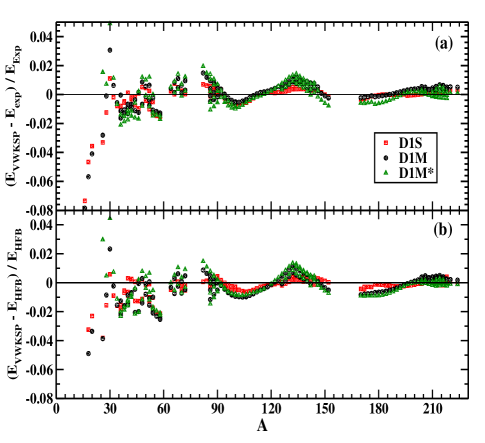
Figure 1: Relative difference between binding energies calculated from VWKSP approach with HFB method in harmonic oscillator basis and their experimental values for $\sim 160$ even-even nuclei spread across the whole nuclear chart using D1M, D1S and D1M* Gogny forces.

III Results and Discussions

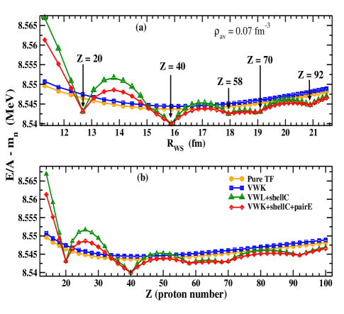
Figure 2: Binding energy per particle subtracted by the free nucleon mass for inner crust of neutron star calculated with D1M* force as a function of radius of the WS cell in panel (a) and as a function of proton number $Z$ in panel (b) at average density $\rho_{\rm av}=0.07$ fm^-3.

III.1 Finite Nuclei

Table 1: Binding energies of 10 different nuclei across the nuclear chart calculated with VWKSP method and compared with their experimental values along with the ones calculated with Hartree-Fock-Bogoliubov (HFB) method in harmonic oscillator basis using D1M* Gogny force.

Nucl.($\rm{}_{Z}^{A}X_{N}$)	$\rm{}_{12}^{32}Mg_{20}$	$\rm{}_{20}^{40}Ca_{20}$	$\rm{}_{20}^{50}Ca_{30}$	$\rm{}_{40}^{90}Zr_{50}$	$\rm{}_{50}^{100}Sn_{50}$	$\rm{}_{62}^{142}Sm_{80}$	$\rm{}_{80}^{176}Hg_{96}$	$\rm{}_{82}^{208}Pb_{126}$	$\rm{}_{84}^{216}Po_{132}$	$\rm{}_{92}^{224}U_{132}$
Expt.	-249.849	-342.052	-427.490	-783.892	-824.794	-1176.614	-1369.743	-1636.430	-1675.904	-1710.285
VWKSP	-251.665	-338.010	-429.318	-784.834	-818.355	-1174.188	-1357.301	-1636.241	-1679.186	-1708.199
HFB	-248.848	-342.546	-424.996	-783.138	-826.542	-1174.549	-1364.428	-1636.729	-1671.738	-1706.392

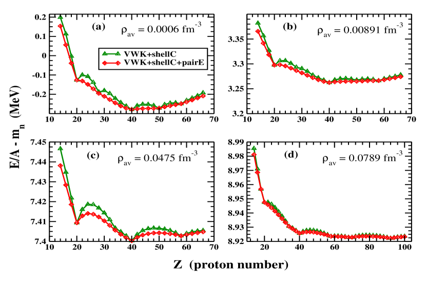
Figure 3: Binding energy per particle for inner crust of neutron star subtracted by free nucleon mass calculated at different average densities mentioned in different panels using VWK approach with shell correction and pairing are plotted as a function of proton number $Z$ for D1M* Gogny force in the spherical WS approximation.

Before applying the VWK method with shell and pairing correction (VWKSP) to the inner crust, we take recourse to testing it for finite nuclei. For this purpose we have used three different Gogny forces, namely, D1S, D1M and D1M^∗. We want to recall here that all three forces mentioned previously belong to D1 family of Gogny forces with the interaction given by Eq. (1). As it was pointed out before, the new D1M^∗ force was built with the aim to be able to predict a maximum NS mass of about 2$M_{\odot}$ and, at the same time, describe finite nuclei with a quality similar to that found using the D1M interaction. To this end, starting with the D1M force, the eight parameters that determine the finite-range part of the force were modified as follows. The saturation density, binding energy per nucleon, incompressibility coefficient and effective mass in symmetric nuclear matter, as well as the symmetry energy at a subsaturation density ($\rho=0.1$ fm^-3) in the isovector sector, were kept fixed to the values predicted by the D1M force. The two combinations of $W_{i},B_{i},H_{i}$ and $M_{i}\ (i=1,2)$, which determine the strength of the pairing force in the $S=0,T=1$ channel, were also kept at the same value as in the original D1M force. In this way seven out of the eight parameters were determined. The last parameter, chosen to be $B_{1}$, was used to modify the slope of the symmetry energy at saturation, which in turn determines the maximum mass of the neutron star. Finally, the strength of the zero-range part of the force and the spin-orbit strength in Eq.(1) were fine tuned for improving the description of finite nuclei (see Ref.Gonzalez-Boquera et al. (2018) for further details).

We have calculated the binding energies of a set of even-even spherical nuclei and compared them with their experimental values in Fig 1(a). In this figure we plot the relative difference in the binding energy for $\sim 160$ even-even nuclei spread across the entire nuclear chart, calculated with the VWKSP method using the Gogny forces mentioned before from their experimental values. One can observe that the differences for the lighter nuclei are on the higher side compared to those for heavier nuclei. This is a typical feature of the mean-field approximation, which works better with a relatively large number of particles in the system. From this panel we see that for mass numbers larger than $A\sim 30$ the VWKSP energies are scattered around the experimental values reproducing them within a 2$\%$ of accuracy. In order to validate our VWKSP method to predict binding energies, we compare our results with the ones obtained using the standard HFB method, which is the benchmark for the theoretical ground-state binding energies with effective forces. The relative differences between the HFB and VWKSP methods are plotted in Fig. 1(b). They differences are quite small, less than 2$\%$ almost throughout the entire nuclear chart apart from few nuclei in the lighter region. In Table 1, a representative subset of these nuclei is provided with their binding energies computed with VWKSP method using the D1M* interaction and their comparison with the experimental values as well as with the corresponding HFB results. Overall the agreement is satisfactory. These tests in the finite nuclear sector provide us the much needed confidence to apply VWKSP method for the case of inner crust of NS.

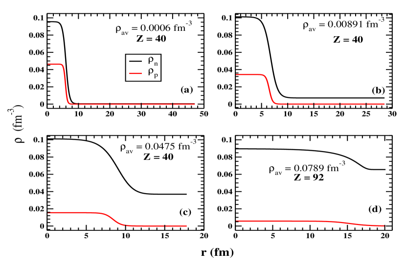
Figure 4: Same as Fig. 3 but for neutron and proton density profiles inside the WS cell.

III.2 Inner crust of Neutron Stars

We start the calculation of inner crust by choosing different average densities $\rho_{\rm av}$ ranging from 0.0003 fm^-3 to 0.08 fm^-3. Some of the choices are taken from the article by Negele and Vautherin Negele and Vautherin (1973). For each average density we search the optimal configuration, i.e., neutron and proton numbers which minimize the energy per particle in the WS cell using the VWKSP method. To this end, we proceed in two steps. In the first one, for an even proton number $Z$ we determine the neutron number $N$ from the $\beta$-equilibrium condition (Eq. 11), which also determines the radius of WS cell. In the second step we scan the energy per particle as a function of $Z$ to obtain the global minimum. In panel (a) of Fig. 2, we plot the energy per particle (subtracted by free nucleon mass, $m_{n}=939$ MeV) as a function of radius of the WS cell, $R_{WS}$, for an average density $\rho_{\rm av}=0.07$ fm^-3 using the D1M* interaction. We plot the same quantity as a function of proton number $Z$ in Fig. 2(b). The orange lines with circles represent the pure Thomas-Fermi (TF) calculation. Being a semiclassical calculation in nature, the energy per particle varies smoothly with $N$ and $Z$ in this case. The blue lines with the squares represent the VWK calculation, where the $\hbar^{2}$-correction is added to the TF energy perturbatively. The green lines with triangles correspond to the results when the shell correction is added further, perturbatively. Clearly this quantal effect makes the graphs unsmooth in nature and distinct local minima appear at conventional magic numbers like $Z=20$ or 40, but there also appear few other magic numbers at $Z=58,70,92$ and 138 (the latest not shown in Fig. 2). The red lines with diamonds correspond to added pairing energy on top of the shell correction. This somewhat smoothens the lines compared to those only with shell correction. The global minimum appears at $Z=40$ after incorporation of all the corrections, which describes the optimal configuration of the crust at $\rho_{\rm av}=0.07$ fm^-3 calculated with the D1M* interaction. This systematic study demonstrates the importance of quantal effects to determine the configuration of the inner crust of neutron star. Notice that the local minima, which correspond to magic proton numbers, are unaffected by pairing correlations as they have an impact only on the open-shell nuclei lying in between the minima. One can notice from Fig. 2 that with increase in proton number the size of the WS cell does not increase linearly. When the proton number increases in a WS cell of given density, the neutron number also increases to maintain the $\beta$-equilibrium and, therefore, the size of the cell, which is determined by the mass number, also grows.

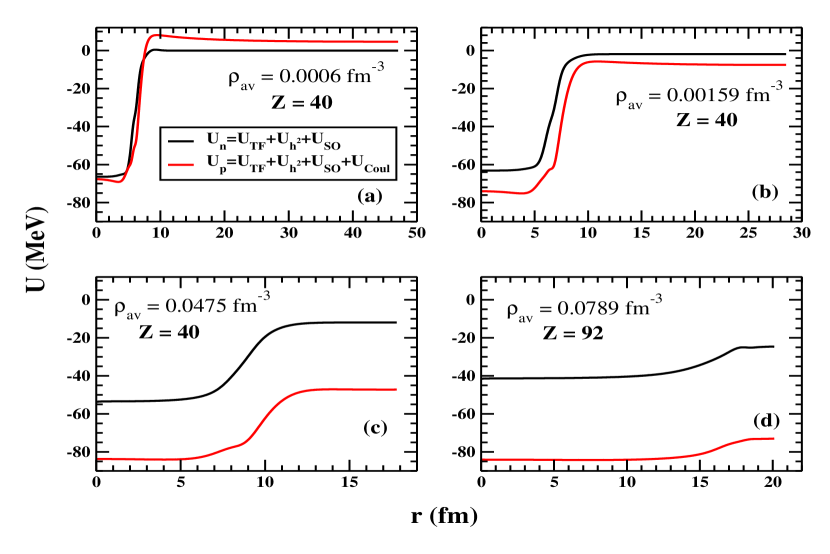
Figure 5: Same as Fig. 3 but for neutron and proton potentials inside the WS cell.

In Fig. 3 we plot the energy per particle subtracted by the free nucleon mass as a function of proton number $Z$ for four different $\rho_{\rm av}$ values using the D1M* interaction. The green lines with the triangles correspond to VWK calculation along with shell correction added perturbatively and the red lines with diamonds correspond to VWKSP calculation, which also includes pairing effects. The general feature one can observe here is that addition of pairing somewhat smoothens the quantal effects throughout the average density range considered in the four panels. At $\rho_{\rm av}=0.0006$ fm^-3 (see Fig. 3(a)) only with shell correction, one can observe the appearance of conventional magic numbers like $Z=20,28,40,50$. However, there is also a hint of local minimum at $Z=58$. Due to the presence of the neutron gas, the appearance of the magic numbers similar to those of finite nuclei gets blurred by the time one reaches a higher average density (for example $\rho_{\rm av}=0.00891$ fm^-3 in Fig. 3(b)) and the appearance of magic numbers like $Z=28$ or 50 gets completely washed away when one reaches even higher average density (say, $\rho_{\rm av}=0.0475$ fm^-3 depicted in Fig. 3(c)). The global minima appear at $Z=40$ for average densities upto $\sim 0.08$ fm^-3, where the minimum shifts to $Z=92$ (see Fig. 3(d)). One can also notice that the effects of shell correction get diluted when one shifts to higher average densities (notice that the vertical scales of the panels of Fig. 3 are different for different panels). Overall, the inclusion of quantal effects in the energy is quite crucial for the inner crust of neutron star. We must mention here is that, as a general feature, the semiclassical energy per particle in a WS cell varies very slowly with the proton number. In spite of the larger fluctuations after incorporation of shell and pairing energy emerge, the values of the total energy of the system are very similar for varying number of protons. This implies that determination of minimal energy configuration corresponding to the inner crust of neutron star is a delicate problem from the numerical point of view.

Table 2: Radius of the WS cell $R_{WS}$, its corresponding neutron number $N$, proton number $Z$, energy per particle subtracted by nucleon mass $E/A-m_{n}$, pressure $P$, chemical potentials of neutron ($\mu_{n}$), proton ($\mu_{p}$) and electron ($\mu_{e}$) at different average densities $\rho_{\rm av}$ of inner crust of NS corresponding to the minimum energy configuration for D1S, D1M and D1M* Gogny interactions. We have used $m_{n}=939$ MeV.

	$\rho_{\rm av}$	$R_{WS}$	$N$	$Z$	$E/A-m_{n}$	$P$	$\mu_{n}$	$\mu_{p}$	$\mu_{e}$
	(fm-3)	(fm)			(MeV)	(MeV fm-3)	(MeV)	(MeV)	(MeV)
D1S	0.0004	50.0488	170.0538	40	-0.85386	0.00052	0.5105	-25.0660	25.5769
	0.0006	48.1364	240.3249	40	-0.36003	0.00067	0.8037	-25.7910	26.5951
	0.000879	46.1657	322.2734	40	0.05280	0.00092	1.1274	-26.6055	27.7329
	0.00159	42.6967	478.4050	40	0.66983	0.00170	1.7578	-28.2341	29.9917
	0.00373	36.8371	741.0056	40	1.67778	0.00505	3.0441	-31.7328	34.7766
	0.00577	33.5312	871.1931	40	2.31735	0.00926	3.9311	-34.2858	38.2171
	0.00891	30.1276	980.6055	40	3.07788	0.01714	5.0082	-37.5434	42.5520
	0.0204	23.6452	1089.6526	40	4.98537	0.05594	7.7295	-46.5564	54.2863
	0.03	20.7605	1084.4102	40	6.13499	0.09690	9.3633	-52.5260	61.8894
	0.0475	17.5449	1034.5676	40	7.77519	0.18563	11.6701	-61.7009	73.3706
	0.06	12.7870	505.4683	20	8.73363	0.25872	12.9645	-67.4367	80.4012
D1M	0.0004	48.7506	154.1277	40	-0.86383	0.00057	0.4688	-25.7906	26.2594
	0.0006	46.7373	216.5842	40	-0.36546	0.00073	0.7844	-26.6088	27.3930
	0.000879	44.6674	288.1330	40	0.05627	0.00100	1.1325	-27.5327	28.6653
	0.00159	41.0245	419.8488	40	0.69759	0.00185	1.8132	-29.4046	31.2174
	0.00373	34.9033	624.3484	40	1.76817	0.00548	3.2011	-33.5087	36.7096
	0.00577	31.5165	716.6228	40	2.45137	0.00995	4.1402	-36.5290	40.6694
	0.00891	28.1298	790.7460	40	3.25485	0.01801	5.2393	-40.3485	45.5880
	0.0204	25.1930	1308.3346	58	5.16037	0.05291	7.7310	-49.7482	57.4793
	0.03	22.3713	1348.9628	58	6.19822	0.08396	8.9590	-55.8469	64.8064
	0.0475	19.4933	1415.8068	58	7.52030	0.14037	10.4099	-64.1245	74.5343
	0.06	18.2139	1460.6204	58	8.21455	0.18126	11.1399	-68.7630	79.9025
	0.0789	19.5763	2387.4758	92	9.04198	0.24948	12.0330	-74.6456	86.6787
D1M*	0.0004	49.0468	157.6882	40	-0.74943	0.00056	0.4855	-25.6148	26.1005
	0.0006	47.0450	221.6858	40	-0.27892	0.00072	0.7993	-26.4144	27.2135
	0.000879	44.9802	295.0745	40	0.12384	0.00098	1.1463	-27.3191	28.4656
	0.00159	41.3408	430.5692	40	0.74518	0.00183	1.8248	-29.1535	30.9779
	0.00373	35.2332	643.3648	40	1.79723	0.00543	3.2033	-33.1619	36.3650
	0.00577	31.8661	742.0830	40	2.47121	0.00983	4.1300	-36.0917	40.2217
	0.00891	28.5108	824.9535	40	3.26236	0.01770	5.2060	-39.7706	44.9766
	0.0204	22.6141	948.2304	40	5.12315	0.05114	7.5829	-49.2004	56.7834
	0.03	20.2603	1005.0806	40	6.12660	0.08046	8.7544	-54.6898	63.4438
	0.0475	17.8000	1082.1295	40	7.40033	0.13496	10.1676	-62.1776	72.3449
	0.06	16.6427	1118.5374	40	8.07662	0.17845	10.9405	-66.5598	77.5002
	0.07	15.8808	1134.3594	40	8.53993	0.22176	11.5152	-69.8479	81.3629
	0.0789	20.0985	2591.2263	92	8.92225	0.26701	12.0208	-72.7213	84.7418

In Fig. 4 we plot the density profiles for neutrons and protons inside the WS cell at four different $\rho_{\rm av}$ values as the ones considered in Fig. 3 corresponding to their minimum energy configuration computed with the D1M* Gogny force. The black solid lines correspond to the neutron density profile and the red lines denote the ones for protons. For each average density we mention the number of protons corresponding to the minimum energy configuration described before in Fig. 3. By close inspection one can notice that at an average density as low as $0.0006$ fm^-3 (depicted in Fig. 4(a)), the density profiles for both protons and neutrons resemble very much to those in finite nuclei, maintaining a constant density from the center to certain extent and then fall down in a very short distance as compared with the size of the WS cell. Although not visible in Fig. 4(a), the neutron density profile maintains a feeble presence throughout the whole WS cell owing to the neutron gas, unlike finite nuclei where it vanishes. The proton density profile behaves differently and vanishes inside the WS cell, because at such low average densities there are no dripped protons in the inner crust. With increasing average density of the WS cell, the neutron gas becomes more and more prominent. More quantitatively, if we take the case of lowest average density $\rho_{\rm av}=0.0006$ fm^-3 considered here, the neutron and proton densities remain constant, respectively, at $\sim$ 0.095 fm^-3 and $\sim$ 0.045 fm^-3 from the center of the WS cell to about radius $r\sim 8$ fm and they fall almost to zero at $r\sim 10$ fm. For a large average density such as $0.0789$ fm^-3 (represented in Fig. 4(d)), the neutron density profile reaches $0.09$ fm^-3 at the center and attenuates to 0.065 fm^-3 at $r\sim 17$ fm. However, in this case the proton density remains constant at 0.01 fm^-3 starting from the center and vanishes at $r\sim 17$ fm. So, the WS cell is filled with dense neutron gas for this case and protons tend to spread in the whole WS cell. A gradual evolution can be observed through the intermediate average densities depicted in Fig. 4. The central value of the neutron density remains roughly constant and the diffuseness increases when the $\rho_{\rm av}$ in the WS cell increases. However, the proton densities behave a little bit differently; the central density decreases and the diffuseness increases when the average density grows. This is because at high average densities, protons tend to maintain an almost uniform distribution in the whole WS cell in an attempt to reduce the Coulomb energy.

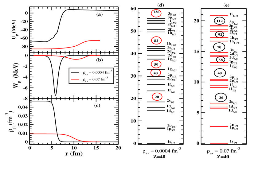
Figure 6: Single-particle potential, spin-orbit potential and density distributions are compared for protons in inner crust of neutron star at $\rho_{\rm av}=0.0004$ fm^-3 and 0.07 fm^-3, respectively, in panels (a-c) calculated with D1M* interaction. The boxes are truncated at $r=20$ fm for better comparison. In panels (d-e), the single particle energy levels for protons calculated with the same interaction are compared. Possible appearance of magic numbers are encircled.

In Fig. 5 we plot the single-particle potentials for neutrons and protons inside the WS cell corresponding to the minimum energy configurations for the different average densities considered in Figs. 3 and 4 computed using the D1M* interaction. As indicated in the figure, these potentials consist of the self-consistent TF part plus the $\hbar^{2}$ and the spin-orbit contributions to the mean field added perturbatively (see Appendix A for further details). These proton potentials also include the contribution from Coulomb interaction taking into account the contribution of the electrons. We use this form as $U_{q}$ ($q=n$ for neutrons and $p$ for protons) of the potential in the Schrödinger equation (6), which allows one to find the single-particle levels needed to compute the shell and pairing corrections to the semiclassical energy through the Strutinsky integral method and BCS approximation, respectively. These potentials, however, show trends different from the case of finite nuclei, especially in larger average densities. This is due to the presence of the denser neutron and electron gases, which deeply modify the potentials. The depths of the proton potentials decrease with increase in the average density of the WS cell. For example, at average density $\rho_{\rm av}=0.0006$ fm^-3 (in Fig. 5(a)), the depth of the proton potential is $\sim-65$ MeV and even has a Coulomb barrier of $\sim 10$ MeV before attenuating at $r\sim 20$ fm. Because of the screening of the proton potential in the crust by electrons, the Coulomb potential is reduced compared to the case of terrestrial finite nuclei. The depth of the neutron potential is $\sim-65$ MeV and it goes to a constant value corresponding to the single-particle potential of the neutron gas at $r\sim 10$ fm. On the other extreme of considered average density $\rho_{\rm av}=0.0789$ fm^-3 (represented in Fig. 5(d)), the depth of the proton potential is $\sim-85$ MeV at the center of the cell, which freezes to $\sim-70$ MeV at $r\sim 17$ fm making the effective depth of only about $\sim-15$ MeV. For neutrons, the potential at the center is $\sim-40$ MeV and attenuates to $\sim-25$ MeV at $\sim 17$ fm. Unlike finite nuclei this situation is very unique, which is due to the existence of the neutron gas that has an important impact not only on the neutrons but also on the protons contained in the WS cell. On the other hand, the frozen value of the neutron potential is much smaller compared to those of protons. This indicates to the smaller chemical potential for neutrons compared to those for protons throughout the whole region of inner crust of neutron stars (see Table 2 for further details).

In Table 2, we summarize the value of WS radius, neutron number $N$ and proton number $Z$ corresponding to their $\beta$-equilibrium configuration, the energy per particle subtracted by the free nucleon mass, pressure and the chemical potentials for neutron, proton and electron respectively, for all the average densities considered in the present work using the D1S, D1M and D1M* interactions. For the D1S interaction, apart from $\rho_{\rm av}=0.06$ fm^-3, for all other average densities the minimum energy configuration appears at $Z=40$ and it becomes $Z=20$ for $\rho_{\rm av}=0.06$ fm^-3. For D1M interaction over the growing $\rho_{\rm av}$ minimum energy configuration shifts from $Z=40$ to $Z=58$ at $\rho_{\rm av}=0.0204$ fm^-3 and at $\rho_{\rm av}=0.0789$ fm^-3 it appears at $Z=92$. For D1M* for all lower average densities the minimum energy configuration corresponds to $Z=40$ that shifts to $Z=92$ at $\rho_{\rm av}=0.0789$ fm^-3, which is almost the transition density estimated by our inner crust calculation using the D1M* interaction.

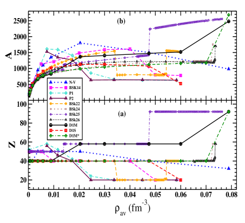
Figure 7: Proton number $Z$ and total number of nucleons $A$ corresponding to the $\beta$-equilibrium configuration as a function of the inner crust density $\rho_{av}$ for D1M, D1S and D1M* interactions in panels (a) and (b), respectively. We also provide the respective numbers predicted by the calculation of Negele and Vautherin (N-V) Negele and Vautherin (1973), P1, P2 Baldo et al. (2007) and BSk22-BSk26 Pearson et al. (2018) for comparison.

We have seen that when shell effects are added to the semiclassical calculation of the energy per particle in WS cells in the inner crust of neutron stars, several local minima appear as a function of the proton number considered in the cell. The atomic numbers corresponding to these minima depend on the average density of the WS cell and change from the standard magic numbers in finite nuclei to the major shell closures in a spherical box or in a Woods-Saxon potential without spin-orbit contribution. To get more insight about this evolution of magic numbers predicted in WS cells, we consider two specific average densities from the two ends of the density range considered, namely $\rho_{\rm av}=0.0004$ fm^-3 and $\rho_{\rm av}=0.07$ fm^-3 and compute their optimal configurations using the D1M* interaction. From Table 2 one can see that, for both these average densities the minimum energy configuration corresponds to $Z=40$. In panel (a) of Fig. 6 we plot the proton potentials for the aforementioned average densities. For $\rho_{\rm av}=0.0004$ fm^-3 the single-particle proton potential resembles very much to the ones corresponding to finite nuclei. The protons seem to be concentrated in a small region of the WS cell upto about $\sim 5$ fm. They are affected very little by the diluted electron gas, which is smeared throughout the whole WS cell (see Fig. 6(c)). For the higher average density considered in this example ($\rho_{\rm av}=0.07$ fm^-3) the radius of the WS cell is much smaller, $R_{WS}\sim 16$ fm. This significantly reduces the Coulomb effects in the WS cell. In this scenario the proton potential is almost due to the nuclear part, which is deep and and almost uniform. It is attenuated from $\sim-85$ MeV at the center to $\sim-70$ MeV at the edge, which is quite similar to a shallow Woods-Saxon potential with a large radius and diffuseness. The form factors of the spin-orbit potential (Eq. (30)) are also very different at these two average densities considered. This is due to the fact that they are determined by the gradients of the neutron and proton densities, which are much larger for $\rho_{\rm av}=0.0004$ fm^-3 compared to those for $\rho_{\rm av}=0.07$ fm^-3. These spin-orbit potentials are displayed in the panel (b) of Fig. 6. The spin-orbit potential is similar to the cases of finite nuclei for the lower average density considered here, however, it is strongly damped and shifted outwards for the case of $\rho_{\rm av}=0.07$ fm^-3, which is in agreement with previous findings for the change of the spin-orbit potential near the neutron drip-line Von-Eiff et al. (1995); Estal et al. (1999); Del Estal et al. (2001). As a consequence of the different mean-field $U_{p}$ and spin-orbit potential $W_{p}$ entering in the Schrödinger equation (Eq. (6)), the level schemes are very different for these two average densities. For $\rho_{\rm av}=0.0004$ fm^-3 the magicity appears at $Z=20,40,50$ or 82, as in standard nuclei, with quite strong gaps. In the high density case, however, as the spin-orbit effect gets much more diluted, the magicity is quite similar to the one on a shallow Woods-Saxon potential without spin-orbit with major shell closures at $Z=20,40,58,70,90,112$ etc. This is demonstrated in Fig. 6(d) and 6(e).

We plot in Fig. 7 the number of protons in panel (a) and total number of baryons in panel (b) within the WS cell corresponding to the $\beta$-equilibrium configuration as a function of the crustal average density. We compare the results obtained with the Gogny forces used in this work with other calculations existing in the literature at the WS level. We include in the figure only those calculations where the search of the $\beta$-equilibrium configuration consistent with the interaction used in the calculation has been performed and where the shell corrections have been explicitly taken into account. The number of protons of the selected configurations (see Fig. 7(a)) lie in the range between $Z=20$ and 50 for most of the interactions, with preferences at $Z=20,40$ or 50. D1M stands out among all the interactions considered, having a preference at $Z=58$ for most of the configurations in the density range considered. The configuration corresponding to $\rho_{av}\sim 0.08$ fm^-3 reaches $Z=92$ for D1M and D1M*, which is quite different from the others, though it was also predicted by the calculation using the BSk25 Skyrme force Pearson et al. (2018). The total number of baryons shown in Fig. 7(b) depends a great deal on the symmetry energy of the respective interactions. This is the reason why even with the same proton numbers, different interactions predict different neutron content. We want to mention here that there exist in the literature some other studies of the inner crust within the WS approximation using Skyrme Grill et al. (2011); Pastore et al. (2011) or Gogny Than et al. (2011) interactions. However, these works, mainly devoted to the study of the pairing properties in the inner crust, use the configurations obtained by Negele and Vautherin Negele and Vautherin (1973) without searching for the $\beta$-equilibrated configurations associated with the force.

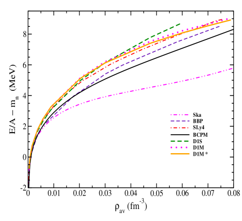
Figure 8: Energy per particle for inner crust of neutron star subtracted by free nucleon mass as a function of density for D1M, D1S and D1M* Gogny forces along with few very successful interactions like BBP, Sly4, BCPM and Ska.

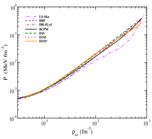
Figure 9: Pressure as a function of density for the inner crust of neutron star using the same set of interactions as Fig. 8.

In Figs. 8 and 9, we plot the energy per particle subtracted by the nucleon mass and the pressure, respectively, as a function of the density in the range relevant for the inner crust of neutron stars for the Gogny D1S, D1M and D1M* interactions. For comparison we also provide the same quantities obtained with the Compressible Liquid Drop Model of Baym-Bethe-Pethick (BBP)Baym et al. (1971), the Skyrme Sly4 Chabanat et al. (1998) and Ska Lattimer and Swesty (1991) interactions and with the BCPM energy density functional Baldo et al. (2008, 2010, 2013), which is derived using a microscopic interaction from Brueckner calculations with two and three-body forces supplemented by a phenomenological term. The energy per particle seems to be on the higher side of the figure for all the Gogny interactions compared to the test calculations. Specially at higher densities of the inner crust, D1S predicts higher energies, whereas D1M and D1M* come down in the regime of the Sly4 interaction. As far as the pressure is concerned (Fig. 9), at higher densities D1M and D1M* have a lowering trend compared to others. On the contrary, D1S produces higher pressure. The numerical values of the energy per particle subtracted by the nucleon mass, the pressure as well as the neutron, proton and electron chemical potentials computed with the D1S, D1M and D1M* Gogny forces are also reported in Table 2. We want to mention here that, if we plot the pressure as a function of density for the Gogny forces computed semiclassically with TF or VWK method, the results are almost indistinguishable from the ones we have plotted in Fig. 9 obtained with VWKSP method, which also includes shell and pairing corrections. This points out to the fact that the composition of the inner crust does not play a significant role in the equation of state of the neutron star, which in turn determines its global properties. Out of the three interactions considered here, only D1M* can predict neutron stars with masses of 2$M_{\odot}$. We provide the combined EoS of core and inner crust calculated with the D1M* interaction in Appendix C.

IV Summary and Conclusions

In summary, we have constructed the EoS of the inner crust of neutron stars using the finite-range Gogny forces D1S, D1M and D1M*. For this purpose, we have implemented the semiclassical Variational Wigner-Kirkwood method in the spherical Wigner-Seitz approximation. Further, we use the Strutinsky integral method to add perturbatively the effects of the quantal shell corrections for protons. Pairing correlations are added in the BCS approach with the same Gogny force as the mean field. Details about the theory used in this work are provided in Appendices A and B.

It is found that the quantal effects play a significant role to determine the specific composition of the inner crust of the neutron star. We have seen that in the inner crust of neutron stars the usual shell structures of terrestrial nuclei get washed away at higher average densities, where shell closures are similar to the ones of a Woods-Saxon potential well without the spin-orbit term. In contrast to the composition, we have noticed that the equation of state (pressure-vs-density relation) of the inner crust does not get much influenced by the shell and pairing effects in the inner crust. Therefore, the global properties of the star such as the mass and radius do not get affected either. However, for low-mass neutron stars (below the canonical mass of 1.4$M_{\odot}$), the stellar radius can change by a considerable amount depending on the treatment of the inner crust of neutron stars Baldo et al. (2014), which points out the importance of describing the crust and the core with the same interaction. We have compared our results for the energy and pressure with the ones provided by some popular models of the inner crust available in the literature. In our calculations, special attention is paid to the D1M* interaction, which was proposed for astrophysical calculations. We have obtained a unified EoS for inner crust and core in Appendix C, which can be used for astrophysical simulations using the D1M* force.

V Acknowledgments

C.M., M.C. and X.V. were partially supported by Grant FIS2017-87534-P from MINECO and FEDER, and Project MDM-2014-0369 of ICCUB (Unidad de Excelencia María de Maeztu) from MINECO. J. N. D. acknowledges support from the Department of Science and Technology through grant no. EMR/2016/001512.

APPENDICES

Appendix A The Variational Wigner-Kirkwood method with shell and paring corrections

The quasilocal energy density functional theory for a finite-range force, established in Ref. Soubbotin et al. (2003) (also see Refs. Gridnev et al. (2017); Behera et al. (2013, 2016)), allows one to write the energy density in a quasilocal form as

$$\mathcal{H}\equiv\mathcal{H}(\rho_{n},\rho_{p},\tau_{n},\tau_{p},\vec{J}_{n},\vec{J}_{p}),$$ (13)

where the local particle, kinetic energy and spin densities entering in (13) are obtained in the spirit of the Kohn-Sham scheme from a Slater determinant wave function of single-particle orbitals $\phi_{i}$ as

$$\rho_{q}(\vec{r})=\sum_{i=1}^{A_{q}}\sum_{\sigma}\mid{\phi_{i}(\vec{r},\sigma,q)}\mid^{2},$$

$$\tau_{q}(\vec{r})=\sum_{i=1}^{A_{q}}\sum_{\sigma}\mid{\vec{\nabla}\phi_{i}(\vec{r},\sigma,q)}\mid^{2},$$

$${\vec{J}}(\vec{r})=i\sum_{i=1}^{A_{q}}\sum_{\sigma\sigma^{\prime}}\phi^{*}(\vec{r},\sigma,q)\left[(\vec{\sigma})_{\sigma\sigma^{\prime}}\times\vec{\nabla}\right]\phi_{i}(\vec{r},\sigma,q).$$ (14)

The orbitals $\phi_{i}$ that determine these densities (A) are the solutions of the single-particle equations

$${h}\phi_{i}=\left\{-\vec{\nabla}\frac{\hbar^{2}}{2m_{q}^{*}(\vec{r})}\vec{\nabla}+U_{q}(\vec{r})-i\vec{W}_{q}(\vec{r})(\vec{\nabla}\times\vec{\sigma})\right\}\phi_{i}=\epsilon_{i}\phi_{i}.$$

The effective mass $m_{q}^{*}$, the mean-field $U_{q}$ and spin-orbit potential $\vec{W}_{q}$ in (A) are defined as

$$\frac{\hbar^{2}}{2m_{q}^{*}}=\frac{\delta\mathcal{H}}{\delta\tau_{q}},\ \ U_{q}=\frac{\delta\mathcal{H}}{\delta\rho_{q}},\ \ \vec{W}_{q}=\frac{\delta\mathcal{H}}{\delta\vec{J}_{q}}.$$ (16)

They are computed from the energy density (13) with the definitions (A) by applying the variational principle to the single particle orbitals $\phi_{i}$.

In the case of the Gogny interaction (1) the quasilocal energy density (13) can be written as

$$\mathcal{H}=\frac{\hbar^{2}}{2m}(\tau_{n}+\tau_{p})+\mathcal{H}_{dir}+\mathcal{H}_{exch}+\mathcal{H}_{zr}+\mathcal{H}_{coul}+\mathcal{H}_{SO},$$ (17)

where the different contributions are given by

$$\mathcal{H}_{dir}=\frac{1}{2}\sum_{i=1}^{2}\int d\vec{r^{\prime}}\left\{\left(W_{i}+\frac{B_{i}}{2}\right)\rho(\vec{r})\rho(\vec{r^{\prime}})-\left(H_{i}+\frac{M_{i}}{2}\right)\left[\rho_{n}(\vec{r})\rho_{n}(\vec{r^{\prime}})+\rho_{p}(\vec{r})\rho_{p}(\vec{r^{\prime}})\right]\right\}e^{-\frac{(\vec{r}-\vec{r^{\prime}})^{2}}{\mu_{i}^{2}}},$$ (18)

$$\mathcal{H}_{zr}=\frac{t_{3}}{4}\rho^{\alpha}(\vec{r})\left[(2+x_{3})\rho^{2}(\vec{r})-(2x_{3}+1)\right.\left.(\rho_{n}^{2}(\vec{r})+\rho_{p}^{2}(\vec{r}))\right],$$ (19)

$$\mathcal{H}_{coul}=\frac{1}{2}\int d\vec{r^{\prime}}\frac{\rho_{p}(\vec{r})\rho_{p}(\vec{r^{\prime}})}{\mid\vec{r}-\vec{r^{\prime}}\mid}-\frac{3}{4}\left(\frac{3}{\pi}\right)^{1\over 3}\rho_{p}^{4\over 3}(\vec{r}),$$ (20)

$$\mathcal{H}_{SO}=-\frac{1}{2}W_{0}\left[\rho(\vec{r})\vec{\nabla}\cdot\vec{J}+\rho_{n}(\vec{r})\vec{\nabla}\cdot\vec{J_{n}}\right.\left.+\rho_{p}(\vec{r})\vec{\nabla}\cdot\vec{J_{p}}\right].$$ (21)

Here, $\rho=\rho_{n}+\rho_{p}$ and $\vec{J}=\vec{J_{n}}+\vec{J_{p}}$ are the total particle and spin densities, respectively.

In the quasilocal reduction of the energy density we shall write the exchange contribution in a local form. To this end, we have to do some approximation to the one-body density matrix, similar to those performed in Refs. Negele and Vautherin (1972, 1975); Campi and Bouyssy (1978, 1979). In this work we use the Extended Thomas-Fermi density matrix derived in Ref. Soubbotin and Viñas (2000), which has been applied to compute the quantal energy of finite nuclei in the quasilocal approximation in Refs. Soubbotin et al. (2003); Gridnev et al. (2017). Using this approximation we can write the exchange energy density as a sum of the Thomas-Fermi (Slater) term

$$\mathcal{H}_{exch,0} = -\frac{1}{2}\sum_{i}\int d\vec{s}e^{-\frac{s^{2}}{\mu_{i}^{2}}}\left\{\left(B_{i}+\frac{W_{i}}{2}\right)\right.\left.\left[\left(\rho_{n}(\vec{r})\frac{3j_{1}(k_{F_{n}}s)}{k_{F_{n}}s}\right)^{2}+\left(\rho_{p}(\vec{r})\frac{3j_{1}(k_{F_{p}}s)}{k_{F_{p}}s}\right)^{2}\right]\right.$$ (22)

$$\left.-\left(M_{i}+\frac{H_{i}}{2}\right)\rho_{n}(\vec{r})\frac{3j_{1}(k_{F_{n}}s)}{k_{F_{n}}s}\rho_{p}(\vec{r})\frac{3j_{1}(k_{F_{p}}s)}{k_{F_{p}}s}\right\},$$

where $k_{F_{q}}=(3\pi^{2}\rho_{q}(\vec{r}))^{1/3}$ is the local Fermi momentum for each type of nucleon and $j_{1}$ is the spherical Bessel function, plus a corrective $\hbar^{2}$-contribution, which reads

$$\mathcal{H}_{exch,2} = \sum_{q}\frac{\hbar^{2}}{2m_{q}}\left\{(f_{q}-1)\left(\tau_{q}-\frac{3}{5}k_{F_{q}}^{2}\rho_{q}-\frac{1}{4}\Delta\rho_{q}\right)\right.\left.+k_{F_{q}}f_{qk}\left[\frac{1}{27}\frac{(\vec{\nabla}\rho_{q})^{2}}{\rho_{q}}-\frac{1}{36}\Delta\rho_{q}\right]\right\}.$$ (23)

In this equation

$$f_{q}\equiv f_{q}(\vec{r},k)_{k=k_{F_{q}}}\ \ \text{and}\ \ f_{qk}\equiv\left(\frac{\partial f(\vec{r},k)}{\partial k}\right)_{k=k_{F_{q}}}$$ (24)

are the inverse of the position and momentum-dependent effective mass and its derivative with respect to the momentum, both computed at the corresponding local Fermi momentum for each kind of nucleons. The quantity $f_{q}(\vec{r},k)$ that enters in Eq. 23 is defined as

$$f_{q}(\vec{r},k)=1+\frac{m}{\hbar^{2}k}\frac{\partial U_{exch,q}(\vec{r},k)}{\partial k},$$ (25)

where $U_{exch,q}$ is the Wigner transform of the single-particle exchange potential in the TF approximation, which can be written as

$$U_{exch,q}(\vec{r},k) = -\sum_{i}\int d\vec{s}e^{-i\vec{k}\cdot\vec{s}}e^{-\frac{s^{2}}{\mu_{i}^{2}}}\left\{\left(B_{i}+\frac{W_{i}}{2}\right)\rho_{q}(\vec{r})\right.\left.\frac{3j_{1}(k_{F_{q}}s)}{k_{F_{q}}s}\right.$$ (26)

$$- \left.\left(M_{i}+\frac{H_{i}}{2}\right)\left[\rho_{q}(\vec{r})\frac{3j_{1}(k_{F_{q}}s)}{k_{F_{q}}s}\right.\left.+\rho_{q^{\prime}}(\vec{r})\frac{3j_{1}(k_{F_{q^{\prime}}}s)}{k_{F_{q^{\prime}}}s}\right]\right\},$$

where, $q=n,p$ and $q^{\prime}=p,n$. Notice that the exchange potential at TF level is a function not only of the momentum $k$ of the nucleon of type $q$, but also of the position via the dependence of the TF exchange potential on the local Fermi momentum of both, neutrons and protons, $k_{F_{n}}(\vec{r})$ and $k_{F_{p}}(\vec{r})$, respectively.

Combining the total kinetic energy density with the $\hbar^{2}$ part of the exchange energy density (23), one can sort out explicitly the effective mass contribution, which at pure TF level is hidden in the exchange term. In this way we can write

$$\widetilde{\mathcal{E}}=\sum_{q}\left[\frac{\hbar^{2}}{2m}f_{q}\tau_{q}+\frac{\hbar^{2}}{2m}\left\{\left(1-f_{q}\right)\tau_{q,0}-\frac{1}{4}f_{q}\Delta\rho_{q}+k_{F_{q}}f_{qk}\left(\frac{1}{27}\frac{\left(\vec{\nabla}\rho_{q}\right)^{2}}{\rho_{q}}-\frac{1}{36}\Delta\rho_{q}\right)\right\}\right],$$ (27)

where $\tau_{q}=\tau_{q,0}+\tau_{q,2}$ contains the pure TF and $\hbar^{2}$ contributions.

In the $\hbar^{2}$ contribution to the exchange energy (23), $\tau_{q}$ is the semiclassical kinetic energy density for each type of particles, which is obtained from the semiclassical ETF density matrix Soubbotin and Viñas (2000); Gridnev et al. (2017) as

$$\tau_{q}(\vec{r})=\left.\left(\frac{1}{4}\Delta_{R}-\Delta_{s}\right)\widetilde{\rho_{q}}(\vec{R},s)\right|_{s=0}=\frac{3}{5}k_{F_{q}}^{2}s_{q}+\frac{1}{36}\frac{(\vec{\nabla}\rho_{q})^{2}}{\rho_{q}}\left[1+\frac{2}{3}k_{F_{q}}\frac{f_{qk}}{f_{q}}+\frac{2}{3}k_{F_{q}}^{2}\frac{f_{qkk}}{f_{q}}-\frac{1}{3}k_{F_{q}}^{2}\frac{f_{qk}^{2}}{f_{q}^{2}}\right]$$

$$+\frac{1}{4}\Delta\rho\left[1+\frac{2}{9}k_{F_{q}}\frac{f_{qk}}{f_{q}}\right]+\frac{1}{6}\rho_{q}\frac{\Delta f_{q}}{f_{q}}+\frac{1}{6}\frac{\vec{\nabla}\rho_{q}\cdot\vec{\nabla}f_{q}}{f_{q}}\left[1-\frac{1}{3}k_{F_{q}}\frac{f_{qk}}{f_{q}}\right]+\frac{1}{9}\frac{\vec{\nabla}\rho_{q}\cdot\vec{\nabla}f_{qk}}{f_{q}}-\frac{1}{12}\rho_{q}\frac{(\vec{\nabla}f_{q})^{2}}{f_{q}^{2}},$$ (28)

which is a functional of the two kind of local densities $\rho_{q}$ and $\rho_{q^{\prime}}$, the latest owing to the presence of effective mass terms in (A). Therefore, including $\hbar^{2}$ corrections the energy density (17) becomes a functional of the particle densities only.

As explained in Ref. Gridnev et al. (2017), the spin-orbit interaction provides an additional term to the semiclassical ETF density matrix, which allows one to calculate the semiclassical spin density as

$$\vec{J}_{q}(\vec{R})=-i\text{Tr}\left\{\left[\vec{\sigma}\times\left(\frac{\vec{\nabla}_{R}}{2}+\vec{\nabla}_{s}\right)\right]\left(-\frac{im}{2\hbar^{2}}\right)\frac{\rho_{q}}{f_{q}}\vec{\sigma}\cdot(\vec{W}_{q}\times\vec{s})\frac{3j_{1}(k_{F_{q}}s)}{k_{F_{q}}s}\right\}_{s=0}=-\frac{2m}{\hbar^{2}}\frac{\rho_{q}\vec{W}_{q}}{f_{q}},$$ (29)

where, the spin-orbit potential $\vec{W}_{q}$ (see third equation in (16)) is given by

$$\vec{W}_{q}(\vec{r})=\frac{1}{2}W_{0}\left[\vec{\nabla}\rho+\vec{\nabla}\rho_{q}\right].$$ (30)

The spin-orbit term in the density matrix also provides another contribution to the kinetic energy density (A) given by

$$\tau_{q,SO}=\frac{1}{2}\left(\frac{2m}{\hbar^{2}}\right)^{2}\frac{\rho}{f_{q}^{2}}W_{q}^{2}.$$ (31)

Using the spin-density (29) in the spin-orbit energy density (21) and performing a suitable partial integration, one can write the semiclassical spin-orbit energy density, which is actually a $\hbar^{2}$ order quantity, as

$$\mathcal{H}_{SO}=\vec{J}_{n}\cdot\vec{W}_{n}+\vec{J}_{p}\cdot\vec{W}_{p}=-\frac{2m}{\hbar^{2}}\left[\frac{\rho_{n}W_{n}^{2}}{f_{n}}+\frac{\rho_{p}W_{p}^{2}}{f_{p}}\right].\ \ \ \$$ (32)

Appendix B The single-particle potential

In order to describe the quantal energy of a nucleus using a finite-range interaction within a Mic-Mac frame, we shall add perturbatively to the macroscopic part given by the semiclassical energy the shell and pairing corrections. For each type of particles these quantal effects are obtained starting from the mean field obtained semiclassically by performing the variation of the energy density (17) with respect to the neutron or proton densities (see second equation (16)). The $\hbar^{0}$ (TF) part of the single-particle potential consists of the direct and zero-range contributions, which read

$$U_{dir,q}=\sum_{i=1}^{2}\int d\vec{r^{\prime}}\left\{\left(W_{i}+\frac{B_{i}}{2}\right)\rho(\vec{r^{\prime}})-\left(H_{i}+\frac{M_{i}}{2}\right)\rho_{n}(\vec{r^{\prime}})\right\}e^{-\frac{(\vec{r}-\vec{r^{\prime}})^{2}}{\mu_{i}^{2}}},$$ (33)

$$U_{zr,q}=\frac{t_{3}}{2}\rho^{\alpha}(\vec{r})\left[(2+x_{3})\rho(\vec{r})-(2x_{3}+1)\rho_{q}(\vec{r})\right]+\frac{t_{3}\alpha}{2}\rho^{\alpha-1}(\vec{r})\left[(2+x_{3})\rho^{2}(\vec{r})-(2x_{3}+1)(\rho_{n}^{2}(\vec{r})+\rho_{p}^{2}(\vec{r}))\right],$$ (34)

plus the exchange term given by Eq.(22), i.e.,

$$U_{q,0}=U_{dir,q}+U_{exch,q}+U_{zr,q}$$ (35)

and, in the case of protons, also including the contribution of the Coulomb potential

$$U_{coul}=\int d\vec{r^{\prime}}\frac{\rho_{p}(\vec{r^{\prime}})}{\mid\vec{r}-\vec{r^{\prime}}\mid}-\left(\frac{3}{\pi}\right)^{1\over 3}\rho_{p}^{1\over 3}(\vec{r}).$$ (36)

Next we compute the $\hbar^{2}$ contribution to the single-particle potential. Notice that the spin-orbit energy (21) is also a $\hbar^{2}$-order quantity that depends on the particle and spin densities for each type of particles. As mentioned before, the neutron and proton spin-orbit potentials, defined by Eq. (30), come from the variation of Eq. (21) with respect to the spin densities. The spin-orbit energy in Eq. (21) also contributes to the mean field of each type of particles through its variation with respect to the corresponding particle density, which is given as

$$U_{SO}=-\frac{1}{2}W_{0}\left[\vec{\nabla}\cdot\vec{J}(\vec{r})+\vec{\nabla}\cdot\vec{J}_{q}(\vec{r})\right].$$ (37)

Therefore, in order to include the spin-orbit contributions in our formalism, which are essential for describing properly the shell effects through the Strutinsky integral method, the semiclassical expansion of the energy should be pushed, at least, up to $\hbar^{2}$-order.

To obtain the nuclear part of the $\hbar^{2}$ contribution to the single-particle potential, one needs to perform the variation of the combination of the kinetic and second-order exchange energy densities $\widetilde{\mathcal{E}}$ (27) with respect to the neutron or proton densities $\rho_{q}$. To perform this variation one needs to treat the $\tau_{q}$ as an independent variable in $\widetilde{\mathcal{E}}$. So, this $\hbar^{2}$ contribution to the single-particle potential is given by

$$U_{q,2}=\frac{\delta\widetilde{\mathcal{E}}}{\delta\rho_{q}}=\frac{\hbar^{2}}{2m}\left(\frac{\delta f_{q}}{\delta\rho_{q}}\tau_{q}+\frac{\delta f_{q^{\prime}}}{\delta\rho_{q}}\tau_{q^{\prime}}\right)+\frac{\hbar^{2}}{2m}\frac{\delta}{\delta\rho_{q}}\left\{(1-f_{q})\tau_{q,0}+(1-f_{q^{\prime}})\tau_{q^{\prime},0}\right\}$$ (38)

$$+ \frac{\hbar^{2}}{2m}\frac{\delta}{\delta\rho_{q}}\left\{-\frac{1}{4}f_{q}\Delta\rho_{q}-\frac{1}{4}f_{q^{\prime}}\Delta\rho_{q^{\prime}}+k_{F_{q}}f_{qk}\left(\frac{1}{27}\frac{\left(\vec{\nabla}\rho_{q}\right)^{2}}{\rho_{q}}-\frac{1}{36}\Delta\rho_{q}\right)+k_{F_{q^{\prime}}}f_{q^{\prime}k}\left(\frac{1}{27}\frac{\left(\vec{\nabla}\rho_{q^{\prime}}\right)^{2}}{\rho_{q^{\prime}}}-\frac{1}{36}\Delta\rho_{q^{\prime}}\right)\right\}.\ \ \ \ \$$

Now, with the definitions $f_{q}\equiv f_{q}(k=k_{F_{q}},k_{F_{q}},k_{F_{q^{\prime}}})\ \text{and}\ f_{q^{\prime}}\equiv f_{q^{\prime}}(k=k_{F_{q^{\prime}}},k_{F_{q^{\prime}}},k_{F_{q}})$, one can easily obtain

$$\frac{\partial f_{q}}{\partial\rho_{q}}=\frac{\partial f_{q}}{\partial k_{F_{q}}}\frac{\partial k_{F_{q}}}{\partial\rho_{q}}=\left(f_{qk}+f_{qk_{F_{q}}}\right)\frac{1}{3}\frac{k_{F_{q}}}{\rho_{q}}\ \text{and}\ \frac{\partial f_{q^{\prime}}}{\partial\rho_{q}}=f_{q^{\prime}k_{F_{q}}}\frac{1}{3}\frac{k_{F_{q}}}{\rho_{q}}.$$ (39)

Using this the variation of the first term in Eq. (38) is given by,

$$\frac{\hbar^{2}}{2m}\left(\frac{\delta f_{q}}{\delta\rho_{q}}\tau_{q}+\frac{\delta f_{q^{\prime}}}{\delta\rho_{q}}\tau_{q^{\prime}}\right)=\frac{\hbar^{2}}{2m}\frac{1}{3}\frac{k_{F_{q}}}{\rho_{q}}\left\{\left(f_{qk}+f_{qk_{F_{q}}}\right)\tau_{q}+f_{q^{\prime}k_{F_{q}}}\tau_{q^{\prime}}\right\}.$$ (40)

Now taking into account that, $\tau_{q,0}=\frac{3}{5}(3\pi^{2})^{2/3}\rho_{q}^{5/3}$, one can write after some algebraic simplifications,

$$\frac{\hbar^{2}}{2m}\frac{\delta}{\delta\rho_{q}}\left\{(1-f_{q})\tau_{q,0}+(1-f_{q^{\prime}})\tau_{q^{\prime},0}\right\}=\frac{\hbar^{2}}{2m}\frac{1}{3\rho_{q}}\left[5\left\{1-f_{q}-\frac{1}{5}k_{F_{q}}\left(f_{qk}+f_{qk_{F_{q}}}\right)\right\}\tau_{q,0}-f_{q^{\prime}k_{F_{q}}}k_{F_{q}}{\tau_{q^{\prime},0}}\right].$$ (41)

Combining Eq. (41) and (40) one gets,

$$\frac{\hbar^{2}}{2m}\left[\frac{\delta f_{q}}{\delta\rho_{q}}\tau_{q}+\frac{\delta f_{q^{\prime}}}{\delta\rho_{q}}\tau_{q^{\prime}}+(1-f_{q})\tau_{q,0}+(1-f_{q^{\prime}})\tau_{q^{\prime},0}\right]=\frac{\hbar^{2}}{2m}\frac{1}{3\rho_{q}}\left[5\left\{1-f_{q}\right\}\tau_{q,0}+k_{F_{q}}\left(f_{qk}+f_{qk_{F_{q}}}\right)\tau_{q,2}+k_{F_{q}}f_{q^{\prime}k_{F_{q}}}\tau_{q^{\prime},2}\right],$$

where in this equation we use the local kinetic energy density $\tau_{q,2}=\frac{1}{36}\frac{(\vec{\nabla}\rho_{q})^{2}}{\rho_{q}}+\frac{1}{3}\Delta\rho_{q}$. As explained in Refs. Soubbotin and Viñas (2000) and Gridnev et al. (2017), one obtains almost the same $\hbar^{2}$-order energy if in the full kinetic energy density (B) the $\hbar^{2}$ contribution is replaced by its local counterpart.

The contributions of the remaining pieces of Eq.(38), which correspond to the $\hbar^{2}$-part of the single particle potential are given after some algebraic steps by,

$$\frac{\hbar^{2}}{2m}\frac{\delta}{\delta\rho_{q}}\left\{-\frac{1}{4}f_{q}\Delta\rho_{q}-\frac{1}{4}f_{q^{\prime}}\Delta\rho_{q^{\prime}}+k_{F_{q}}f_{qk}\left(\frac{1}{27}\frac{\left(\vec{\nabla}\rho_{q}\right)^{2}}{\rho_{q}}-\frac{1}{36}\Delta\rho_{q}\right)+k_{F_{q^{\prime}}}f_{q^{\prime}k}\left(\frac{1}{27}\frac{\left(\vec{\nabla}\rho_{q^{\prime}}\right)^{2}}{\rho_{q^{\prime}}}-\frac{1}{36}\Delta\rho_{q^{\prime}}\right)\right\}$$ (43)

$$= \Bigg{\{}\left[2k_{F_{q}}\left(f_{qk}+f_{qk_{F_{q}}}\right)-k_{F_{q}}^{2}\left(f_{qkk}+2f_{qkk_{F_{q}}}+f_{qk_{F_{q}}k_{F_{q}}}\right)\right]+\frac{1}{324}\left[10k_{F_{q}}f_{qk}-4k_{F_{q}}^{2}\left(f_{qkk}+f_{qkk_{F_{q}}}\right)\right.$$

$$- \left.k_{F_{q}}^{3}\left(f_{qkkk}+2f_{qkkk_{F_{q}}}+f_{qkk_{F_{q}}k_{F_{q}}}\right)\right]\Bigg{\}}\frac{(\vec{\nabla}\rho_{q})^{2}}{\rho_{q}^{2}}$$

$$- \left\{\frac{1}{6}k_{F_{q}}\left(f_{qk}+f_{qk_{F_{q}}}\right)+\frac{1}{108}\left[10k_{F_{q}}f_{qk}+2k_{F_{q}}^{2}\left(f_{qkk}+f_{qkk_{F_{q}}}\right)\right]\right\}\frac{\Delta\rho_{q}}{\rho_{q}}$$

$$- \frac{1}{162}\left[14k_{F_{q}}k_{F_{q^{\prime}}}f_{qkk_{F_{q^{\prime}}}}+k_{F_{q}}^{2}k_{F_{q^{\prime}}}f_{qkkk_{F_{q^{\prime}}}}\right]\frac{\vec{\nabla}\rho_{q}}{\rho_{q}}\frac{\vec{\nabla}\rho_{q^{\prime}}}{\rho_{q^{\prime}}}$$

$$+ \frac{1}{324}\left[4k_{F_{q}}k_{F_{q^{\prime}}}f_{q^{\prime}kk_{F_{q}}}\frac{\rho_{q^{\prime}}}{\rho_{q}}+18k_{F_{q^{\prime}}}f_{qk_{F_{q^{\prime}}}}-9k_{F_{q^{\prime}}}^{2}f_{qk_{F_{q^{\prime}}}}k_{F_{q^{\prime}}}+2k_{F_{q}}k_{F_{q^{\prime}}}f_{qkk_{F_{q^{\prime}}}}-k_{F_{q^{\prime}}}^{2}k_{F_{q}}f_{qkk_{F_{q^{\prime}}}k_{F_{q^{\prime}}}}\right]\frac{(\vec{\nabla}\rho_{q^{\prime}})^{2}}{\rho_{q^{\prime}}^{2}}$$

$$- \frac{1}{108}\left[\left(9k_{F_{q}}f_{q^{\prime}k_{F_{q}}}+k_{F_{q}}k_{F_{q^{\prime}}}f_{q^{\prime}kk_{F_{q}}}\right)\frac{\rho_{q^{\prime}}}{\rho_{q}}+9k_{F_{q^{\prime}}}f_{qk_{F_{q^{\prime}}}}+k_{F_{q}}k_{F_{q^{\prime}}}f_{qkk_{F_{q^{\prime}}}}\right]\frac{\Delta\rho_{q^{\prime}}}{\rho_{q^{\prime}}}.$$

Here, we have used under the integral sign the rules of functional derivative as,

$$\frac{\delta F[\rho]}{\delta\rho}=\frac{\partial f}{\partial\rho}+\sum_{i=1}^{N}(-1)^{i}\nabla^{(i)}\frac{\partial f}{\partial(\nabla^{(i)}\rho)},$$ (44)

where the functional $F[\rho(r)]$ is defined as,

$$F[\rho(r)]=\int f(\vec{r},\rho(\vec{r}),\vec{\nabla}\rho(\vec{r}),\vec{\nabla}^{(2)}\rho(\vec{r})\cdots)d\vec{r}.$$ (45)

Now, to obtain the binding energy of a set of nuclei including shell and pairing effects, as close as possible to the full HF or HFB values overall, a scaling parameter $\beta_{\scriptscriptstyle KE}$ has been introduced in the $\hbar^{2}$-part of the kinetic energy density $\tau_{q}$. Incorporating this parameter, the kinetic energy density now becomes,

$${\mathcal{H}}_{KE}=\sum_{q}\frac{\hbar^{2}}{2m}f_{q}(\tau_{q,0}+\beta_{\scriptscriptstyle KE}\tau_{q,2}),$$ (46)

and the potential part corresponding to the $\hbar^{2}$ term given in Eq. (B) containing $\tau_{q,2}$ and $\tau_{q^{\prime},2}$ is modified as $\beta_{\scriptscriptstyle KE}\tau_{q,2}$ and $\beta_{\scriptscriptstyle KE}\tau_{q^{\prime},2}$ respectively. Following this procedure, we find $\beta_{\scriptscriptstyle KE}=1.45$, 1.4 and 1.75 for D1S, D1M and D1M* interactions, respectively.

Appendix C EoS for D1M*

Table 3: Equation of state for inner crust and core of NS obtained with D1M* interaction. Here we have used $\mathcal{E}=\frac{E}{A}\cdot\rho$. $X_{p}$, $X_{e}$ and $X_{\mu}$ are proton, electron and muon fraction in the medium respectively.

	$\rho$	$E/A-m_{n}$	$P$	$\mathcal{E}$	$P$	$X_{p}$	$X_{e}$	$X_{\mu}$
	(fm-3)	(MeV)	(MeV fm-3)	(g cm-3)	(erg cm-3)
Crust	0.0004	-0.74943	0.00056	6.6903$\times 10^{11}$	8.9472$\times 10^{29}$	0.20234	0.20234	0.00000
	0.0006	-0.27892	0.00072	1.0040$\times 10^{12}$	1.1545$\times 10^{30}$	0.15285	0.15285	0.00000
	0.000879	0.12384	0.00098	1.4716$\times 10^{12}$	1.5760$\times 10^{30}$	0.11938	0.11938	0.00000
	0.00159	0.74518	0.00183	2.6636$\times 10^{12}$	2.9277$\times 10^{30}$	0.08500	0.08500	0.00000
	0.00373	1.79723	0.00543	6.2557$\times 10^{12}$	8.6995$\times 10^{30}$	0.05853	0.05853	0.00000
	0.00577	2.47121	0.00983	9.6839$\times 10^{12}$	1.5749$\times 10^{31}$	0.05115	0.05115	0.00000
	0.00891	3.26236	0.01770	1.4966$\times 10^{13}$	2.8359$\times 10^{31}$	0.04624	0.04624	0.00000
	0.0204	5.12315	0.05114	3.4334$\times 10^{13}$	8.1938$\times 10^{31}$	0.04048	0.04048	0.00000
	0.03	6.12660	0.08046	5.0545$\times 10^{13}$	1.2891$\times 10^{32}$	0.03827	0.03827	0.00000
	0.0475	7.40033	0.13496	8.0138$\times 10^{13}$	2.1623$\times 10^{32}$	0.03565	0.03565	0.00000
	0.06	8.07662	0.17845	1.0130$\times 10^{14}$	2.8591$\times 10^{32}$	0.03453	0.03453	0.00000
	0.07	8.53993	0.22176	1.1824$\times 10^{14}$	3.5529$\times 10^{32}$	0.03406	0.03406	0.00000
	0.0789	8.92225	0.26701	1.3333$\times 10^{14}$	4.2779$\times 10^{32}$	0.03429	0.03429	0.00000
Core	0.0838	9.11446	0.27042	1.4164$\times 10^{14}$	4.3326$\times 10^{32}$	0.03502	0.03502	0.00000
	0.09	9.35675	0.32190	1.5215$\times 10^{14}$	5.1573$\times 10^{32}$	0.03612	0.03612	0.00000
	0.10	9.76819	0.42733	1.6913$\times 10^{14}$	6.8466$\times 10^{32}$	0.03765	0.03765	0.00000
	0.11	10.21459	0.56487	1.8613$\times 10^{14}$	9.0502$\times 10^{32}$	0.03893	0.03893	0.00000
	0.12	10.70424	0.73946	2.0316$\times 10^{14}$	1.1848$\times 10^{33}$	0.04000	0.04000	0.00000
	0.13	11.23588	0.95653	2.2021$\times 10^{14}$	1.5325$\times 10^{33}$	0.04090	0.04082	0.00008
	0.14	11.77626	1.22382	2.3729$\times 10^{14}$	1.9608$\times 10^{33}$	0.04166	0.04098	0.00068
	0.15	12.36780	1.54275	2.5440$\times 10^{14}$	2.4718$\times 10^{33}$	0.04232	0.04090	0.00141
	0.16	13.02104	1.91706	2.7154$\times 10^{14}$	3.0715$\times 10^{33}$	0.04288	0.04072	0.00216
	0.17	13.73982	2.35077	2.8873$\times 10^{14}$	3.7663$\times 10^{33}$	0.04337	0.04048	0.00289
	0.18	14.52609	2.84784	3.0597$\times 10^{14}$	4.5627$\times 10^{33}$	0.04379	0.04021	0.00358
	0.21	17.29766	4.75742	3.5800$\times 10^{14}$	7.6222$\times 10^{33}$	0.04483	0.03938	0.00545
	0.24	20.69063	7.36949	4.1059$\times 10^{14}$	1.1807$\times 10^{34}$	0.04567	0.03864	0.00704
	0.27	24.69654	10.77234	4.6385$\times 10^{14}$	1.7259$\times 10^{34}$	0.04647	0.03804	0.00843
	0.30	29.29993	15.04513	5.1785$\times 10^{14}$	2.4105$\times 10^{34}$	0.04732	0.03763	0.00969
	0.33	34.48178	20.25854	5.7268$\times 10^{14}$	3.2458$\times 10^{34}$	0.04830	0.03741	0.01089
	0.36	40.22117	26.47535	6.2842$\times 10^{14}$	4.2418$\times 10^{34}$	0.04945	0.03739	0.01207
	0.39	46.49613	33.75094	6.8515$\times 10^{14}$	5.4075$\times 10^{34}$	0.05083	0.03756	0.01327
	0.42	53.28414	42.13356	7.4294$\times 10^{14}$	6.7505$\times 10^{34}$	0.05246	0.03794	0.01451
	0.45	60.56242	51.66452	8.0185$\times 10^{14}$	8.2776$\times 10^{34}$	0.05437	0.03853	0.01584
	0.48	68.30797	62.37829	8.6193$\times 10^{14}$	9.9941$\times 10^{34}$	0.05661	0.03934	0.01727
	0.51	76.49773	74.30242	9.2325$\times 10^{14}$	1.1905$\times 10^{35}$	0.05920	0.04038	0.01882
	0.54	85.10850	87.45746	9.8585$\times 10^{14}$	1.4012$\times 10^{35}$	0.06217	0.04165	0.02053
	0.57	94.11700	101.85674	1.0498$\times 10^{15}$	1.6319$\times 10^{35}$	0.06556	0.04316	0.02240
	0.60	103.49989	117.50632	1.1151$\times 10^{15}$	1.8827$\times 10^{35}$	0.06940	0.04493	0.02447
	0.63	113.23382	134.40496	1.1817$\times 10^{15}$	2.1534$\times 10^{35}$	0.07371	0.04697	0.02674
	0.66	123.29558	152.54446	1.2499$\times 10^{15}$	2.4440$\times 10^{35}$	0.07851	0.04928	0.02923
	0.69	133.66233	171.91034	1.3194$\times 10^{15}$	2.7543$\times 10^{35}$	0.08381	0.05186	0.03195
	0.72	144.31192	192.48320	1.3904$\times 10^{15}$	3.0839$\times 10^{35}$	0.08961	0.05470	0.03491
	0.75	155.22325	214.24048	1.4630$\times 10^{15}$	3.4325$\times 10^{35}$	0.09589	0.05780	0.03809
	0.78	166.37673	237.15886	1.5370$\times 10^{15}$	3.7997$\times 10^{35}$	0.10262	0.06113	0.04148
	0.81	177.75459	261.21683	1.6125$\times 10^{15}$	4.1852$\times 10^{35}$	0.10974	0.06467	0.04507
	0.84	189.34119	286.39706	1.6896$\times 10^{15}$	4.5886$\times 10^{35}$	0.11718	0.06837	0.04881
	0.87	201.12315	312.68832	1.7682$\times 10^{15}$	5.0098$\times 10^{35}$	0.12488	0.07220	0.05268
	0.90	213.08924	340.08655	1.8484$\times 10^{15}$	5.4488$\times 10^{35}$	0.13275	0.07612	0.05663
	0.93	225.23028	368.59505	1.9301$\times 10^{15}$	5.9055$\times 10^{35}$	0.14070	0.08007	0.06063
	0.96	237.53882	398.22395	2.0135$\times 10^{15}$	6.3803$\times 10^{35}$	0.14868	0.08403	0.06464
	0.99	250.00888	428.98910	2.0984$\times 10^{15}$	6.8732$\times 10^{35}$	0.15660	0.08796	0.06863
	1.02	262.63561	460.91087	2.1850$\times 10^{15}$	7.3846$\times 10^{35}$	0.16442	0.09184	0.07258
	1.05	275.41506	494.01278	2.2731$\times 10^{15}$	7.9150$\times 10^{35}$	0.17208	0.09563	0.07645
	1.08	288.34398	528.32039	2.3630$\times 10^{15}$	8.4646$\times 10^{35}$	0.17956	0.09933	0.08023
	1.11	301.41961	563.86039	2.4545$\times 10^{15}$	9.0340$\times 10^{35}$	0.18683	0.10292	0.08391
	1.14	314.63960	600.65982	2.5477$\times 10^{15}$	9.6236$\times 10^{35}$	0.19387	0.10639	0.08749
	1.17	328.00187	638.74563	2.6426$\times 10^{15}$	1.0234$\times 10^{36}$	0.20067	0.10973	0.09094
	1.20	341.50460	678.14433	2.7392$\times 10^{15}$	1.0865$\times 10^{36}$	0.20723	0.11295	0.09428
	1.23	355.14611	718.88173	2.8376$\times 10^{15}$	1.1518$\times 10^{36}$	0.21354	0.11605	0.09749
	1.26	368.92487	760.98288	2.9378$\times 10^{15}$	1.2192$\times 10^{36}$	0.21961	0.11902	0.10059
	1.29	382.83948	804.47197	3.0397$\times 10^{15}$	1.2889$\times 10^{36}$	0.22544	0.12187	0.10356
	1.32	396.88859	849.37238	3.1435$\times 10^{15}$	1.3608$\times 10^{36}$	0.23103	0.12460	0.10643
	1.35	411.07097	895.70663	3.2491$\times 10^{15}$	1.4351$\times 10^{36}$	0.23640	0.12722	0.10918
	1.38	425.38542	943.49646	3.3565$\times 10^{15}$	1.5116$\times 10^{36}$	0.24155	0.12973	0.11182
	1.41	439.83081	992.76285	3.4658$\times 10^{15}$	1.5906$\times 10^{36}$	0.24648	0.13213	0.11435

References

- Haensel et al. (2007) P. Haensel, A. Y. Potekhin, and D. G. Yakovlev, Astrophys. Space Sci. Libr. 326, pp.1 (2007).
- Baym et al. (1971) G. Baym, H. A. Bethe, and C. J. Pethick, Nuclear Physics A 175, 225 (1971).
- Chamel et al. (2015) N. Chamel, A. F. Fantina, J. L. Zdunik, and P. Haensel, Phys. Rev. C 91, 055803 (2015).
- Negele and Vautherin (1973) J. W. Negele and D. Vautherin, Nucl. Phy. A207, 298 (1973).
- Pizzochero et al. (2002) P. M. Pizzochero, F. Barranco, E. Vigezzi, and R. A. Broglia, The Astrophysical Journal 569, 381 (2002).
- Sandulescu et al. (2004) N. Sandulescu, N. Van Giai, and R. J. Liotta, Phys. Rev. C 69, 045802 (2004).
- Baldo et al. (2007) M. Baldo, E. Saperstein, and S. Tolokonnikov, Eur. Phys. J. A 32, 97 (2007).
- Grill et al. (2011) F. Grill, J. Margueron, and N. Sandulescu, Phys. Rev. C 84, 065801 (2011).
- Pastore et al. (2011) A. Pastore, S. Baroni, and C. Losa, Phys. Rev. C 84, 065807 (2011).
- Than et al. (2011) H. S. Than, E. Khan, and N. V. Giai, Journal of Physics G: Nuclear and Particle Physics 38, 025201 (2011).
- Pastore (2015) A. Pastore, Phys. Rev. C 91, 015809 (2015).
- Carreau et al. (2019) T. Carreau, F. Gulminelli, N. Chamel, A. F. Fantina, and J. M. Pearson, arXiv:1912.01265 (2019).
- Gögelein and Müther (2007) P. Gögelein and H. Müther, Phys. Rev. C 76, 024312 (2007).
- Newton and Stone (2009) W. G. Newton and J. R. Stone, Phys. Rev. C 79, 055801 (2009).
- Pais and Stone (2012) H. Pais and J. R. Stone, Phys. Rev. Lett. 109, 151101 (2012).
- Schuetrumpf et al. (2014) B. Schuetrumpf, K. Iida, J. A. Maruhn, and P.-G. Reinhard, Phys. Rev. C 90, 055802 (2014).
- Fattoyev et al. (2017) F. J. Fattoyev, C. J. Horowitz, and B. Schuetrumpf, Phys. Rev. C 95, 055804 (2017).
- Schuetrumpf et al. (2019) B. Schuetrumpf, G. Martínez-Pinedo, M. Afibuzzaman, and H. M. Aktulga, Phys. Rev. C 100, 045806 (2019).
- Horowitz et al. (2004) C. J. Horowitz, M. A. Pérez-García, and J. Piekarewicz, Phys. Rev. C 69, 045804 (2004).
- Watanabe et al. (2009) G. Watanabe, H. Sonoda, T. Maruyama, K. Sato, K. Yasuoka, and T. Ebisuzaki, Phys. Rev. Lett. 103, 121101 (2009).
- Schneider et al. (2013) A. S. Schneider, C. J. Horowitz, J. Hughto, and D. K. Berry, Phys. Rev. C 88, 065807 (2013).
- Horowitz et al. (2015) C. J. Horowitz, D. K. Berry, C. M. Briggs, M. E. Caplan, A. Cumming, and A. S. Schneider, Phys. Rev. Lett. 114, 031102 (2015).
- Oyamatsu (1993) K. Oyamatsu, Nuclear Physics A 561, 431 (1993).
- Onsi et al. (2008) M. Onsi, A. K. Dutta, H. Chatri, S. Goriely, N. Chamel, and J. M. Pearson, Phys. Rev. C 77, 065805 (2008).
- Pearson et al. (2012) J. M. Pearson, N. Chamel, S. Goriely, and C. Ducoin, Phys. Rev. C 85, 065803 (2012).
- Sharma et al. (2015) B. K. Sharma, M. Centelles, X. Viñas, M. Baldo, and G. F. Burgio, Astron. Astrophys. 584, A103 (2015).
- Martin and Urban (2015) N. Martin and M. Urban, Phys. Rev. C 92, 015803 (2015).
- Lim and Holt (2017) Y. Lim and J. W. Holt, Phys. Rev. C 95, 065805 (2017).
- Pearson et al. (2018) J. M. Pearson, N. Chamel, A. Y. Potekhin, A. F. Fantina, C. Ducoin, A. K. Dutta, and S. Goriely, Monthly Notices of the Royal Astronomical Society 481, 2994 (2018).
- Pearson et al. (2019) J. M. Pearson, N. Chamel, A. Y. Potekhin, A. F. Fantina, C. Ducoin, A. K. Dutta, and S. Goriely, Monthly Notices of the Royal Astronomical Society 486, 768 (2019).
- Cheng et al. (1997) K. S. Cheng, C. C. Yao, and Z. G. Dai, Phys. Rev. C 55, 2092 (1997).
- Shen et al. (1998a) H. Shen, H. Toki, K. Oyamatsu, and K. Sumiyoshi, Nuclear Physics A 637, 435 (1998a).
- Shen et al. (1998b) H. Shen, H. Toki, K. Oyamatsu, and K. Sumiyoshi, Progress of Theoretical Physics 100, 1013 (1998b).
- Grill et al. (2012) F. Grill, C. m. c. Providência, and S. S. Avancini, Phys. Rev. C 85, 055808 (2012).
- Grill et al. (2014) F. Grill, H. Pais, C. m. c. Providência, I. Vidaña, and S. S. Avancini, Phys. Rev. C 90, 045803 (2014).
- Bao and Shen (2015) S. S. Bao and H. Shen, Phys. Rev. C 91, 015807 (2015).
- Lattimer et al. (1991) J. M. Lattimer, C. J. Pethick, M.Prakash, and P. Haensel, Phys. Rev. Lett. 66, 2701 (1991).
- Douchin and Haensel (2001) A. Douchin and P. Haensel, Astron. Astrophys. 380, 151 (2001).
- Chamel and Haensel (2008) N. Chamel and P. Haensel, Living Rev. Relativ. 11, 10 (2008).
- Piro (2005) A. L. Piro, The Astrophysical Journal 634, L153 (2005).
- Strohmayer and Watts (2006) T. E. Strohmayer and A. L. Watts, The Astrophysical Journal 653, 593 (2006).
- Steiner and Watts (2009) A. W. Steiner and A. L. Watts, Phys. Rev. Lett. 103, 181101 (2009).
- Sotani et al. (2012) H. Sotani, K. Nakazato, K. Iida, and K. Oyamatsu, Phys. Rev. Lett. 108, 201101 (2012).
- Newton et al. (2012) W. G. Newton, M. Gearheart, and B.-A. Li, The Astrophysical Journal Supplement Series 204, 9 (2012).
- Piekarewicz et al. (2014) J. Piekarewicz, F. J. Fattoyev, and C. J. Horowitz, Phys. Rev. C 90, 015803 (2014).
- Lattimer et al. (1977) J. M. Lattimer, F. Mackie, D. G. Ravenhall, and D. N. Schramm, ApJ 213, 225 (1977).
- Meyer (1989) B. S. Meyer, ApJ 343, 254 (1989).
- Freiburghaus et al. (1999) C. Freiburghaus, S. Rosswog, and F.-K. Thielemann, ApJ 525, L121 (1999).
- Goriely et al. (2005) S. Goriely, P. Demetriou, H.-T. Janka, J. M. Pearson, and M. Samyn, Nuclear Physics A 758, 587 (2005).
- Decharge and Gogny (1980) J. Decharge and D. Gogny, Phys. Rev. C 21, 1568 (1980).
- Berger et al. (1991) J. Berger, M. Girod, and D. Gogny, Computer Physics Communications 63, 365 (1991).
- Gonzalez-Boquera et al. (2017) C. Gonzalez-Boquera, M. Centelles, X. Viñas, and A. Rios, Phys. Rev. C 96, 065806 (2017).
- Gonzalez-Boquera et al. (2018) C. Gonzalez-Boquera, M. Centelles, X. Viñas, and L. Robledo, Physics Letters B 779, 195 (2018).
- Demorest et al. (2010) P. Demorest, T. Pennucci, S. Ransom, M. Roberts, and J. Hessels, Nature 467, 1081 (2010).
- Antoniadis and et. al (2013) J. Antoniadis and et. al, Science 340, 1233232 (2013).
- Cromartie et al. (2019) H. T. Cromartie et al. (2019), eprint 1904.06759.
- (57) URL www-phynu.cea.fr.
- Delaroche et al. (2010) J. P. Delaroche, M. Girod, J. Libert, H. Goutte, S. Hilaire, S. Péru, N. Pillet, and G. F. Bertsch, Phys. Rev. C 81, 014303 (2010).
- Schunck and Robledo (2016) N. Schunck and L. M. Robledo, Reports on Progress in Physics 79, 116301 (2016).
- Chappert et al. (2008) F. Chappert, M. Girod, and S. Hilaire, Physics Letters B 668, 420 (2008).
- Goriely et al. (2009) S. Goriely, S. Hilaire, M. Girod, and S. Péru, Phys. Rev. Lett. 102, 242501 (2009).
- Sellahewa and Rios (2014) R. Sellahewa and A. Rios, Phys. Rev. C 90, 054327 (2014).
- Viñas et al. (2018) X. Viñas, C. Gonzalez-Boquera, M. Centelles, L. Robledo, and C. Mondal, Nuclear Theory 37, 68 (2018).
- Viñas et al. (2019) X. Viñas, C. Gonzalez-Boquera, M. Centelles, C. Mondal, and L. Robledo, Acta Phys. Pol. Proc. Suppl. 12, 705 (2019).
- Lourenço et al. (2020) O. Lourenço, M. Bhuyan, C. H. Lenzi, M. Dutra, C. Gonzalez-Boquera, M. Centelles, and X. Viñas, Phys. Lett. B 803, 135306 (2020).
- Gonzalez-Boquera et al. (2019) C. Gonzalez-Boquera, M. Centelles, X. Viñas, and T. R. Routray, Phys. Rev. C 100, 015806 (2019).
- Fantina, A. F. et al. (2013) Fantina, A. F., Chamel, N., Pearson, J. M., and Goriely, S., A&A 559, A128 (2013).
- Potekhin, A. Y. et al. (2013) Potekhin, A. Y., Fantina, A. F., Chamel, N., Pearson, J. M., and Goriely, S., A&A 560, A48 (2013).
- Pearson et al. (2015) J. M. Pearson, N. Chamel, A. Pastore, and S. Goriely, Phys. Rev. C 91, 018801 (2015).
- Goriely et al. (2010) S. Goriely, N. Chamel, and J. M. Pearson, Phys. Rev. C 82, 035804 (2010).
- Chamel et al. (2007) N. Chamel, S. Naimi, E. Khan, and J. Margueron, Phys. Rev. C 75, 055806 (2007).
- Schuck and Viñas (1993) P. Schuck and X. Viñas, Physics Letters B 302, 1 (1993).
- Centelles et al. (1998) M. Centelles, X. Viñas, M. Durand, P. Schuck, and D. Von-Eiff, Annals of Physics 266, 207 (1998).
- Centelles et al. (2007) M. Centelles, P. Schuck, and X. Viñas, Annals of Physics 322, 363 (2007).
- Soubbotin and Viñas (2000) V. Soubbotin and X. Viñas, Nuclear Physics A 665, 291 (2000).
- Soubbotin et al. (2003) V. B. Soubbotin, V. I. Tselyaev, and X. Viñas, Phys. Rev. C 67, 014324 (2003).
- Strutinsky (1967) V. Strutinsky, Nuclear Physics A 95, 420 (1967).
- Wigner (1932) E. Wigner, Phys. Rev. 40, 749 (1932).
- Kirkwood (1933) J. G. Kirkwood, Phys. Rev. 44, 31 (1933).
- Uhlenbeck and Beth (1936) G. E. Uhlenbeck and E. Beth, Physica 3, 729 (1936).
- Ring and Schuck (1980) P. Ring and P. Schuck, The nuclear many-body problem (Springer, New York-Heidelberg-Berlin, 1980).
- Brack and Bhaduri (1997) B. Brack and P. K. Bhaduri, Semiclassical Physics (Addison-Wesley Publishing Co., 1997).
- Gridnev et al. (2017) K. A. Gridnev, V. B. Soubbotin, X. Viñas, and M. Centelles (2017), eprint 1704.03858.
- Centelles et al. (1990) M. Centelles, X. Viñas, F.Garcias, and M.Barranco, Nucl. Phys. A510, 397 (1990).
- Von-Eiff et al. (1995) D. Von-Eiff, H. Freyer, W. Stocker, and M. Weigel, Physics Letters B 344, 11 (1995).
- Estal et al. (1999) M. D. Estal, M. Centelles, and X. Viñas, Nuclear Physics A 650, 443 (1999).
- Del Estal et al. (2001) M. Del Estal, M. Centelles, X. Viñas, and S. K. Patra, Phys. Rev. C 63, 044321 (2001).
- Chabanat et al. (1998) E. Chabanat, P. Bonche, P. Haensel, J. Meyer, and R. Schaeffer, Nucl. Phys. A635, 231 (1998).
- Lattimer and Swesty (1991) J. M. Lattimer and D. F. Swesty, Nuclear Physics A 535, 331 (1991).
- Baldo et al. (2008) M. Baldo, P. Schuck, and X. Viñas, Physics Letters B 663, 390 (2008).
- Baldo et al. (2010) M. Baldo, L. Robledo, P. Schuck, and X. Viñas, Journal of Physics G: Nuclear and Particle Physics 37, 064015 (2010).
- Baldo et al. (2013) M. Baldo, L. M. Robledo, P. Schuck, and X. Viñas, Phys. Rev. C 87, 064305 (2013).
- Baldo et al. (2014) M. Baldo, G. F. Burgio, M. Centelles, B. K. Sharma, and X. Viñas, Phys. Atom. Nucl. 77, 1157 (2014).
- Behera et al. (2013) B. Behera, X. Viñas, M. Bhuyan, T. R. Routray, B. K. Sharma, and S. K. Patra, Journal of Physics G: Nuclear and Particle Physics 40, 095105 (2013).
- Behera et al. (2016) B. Behera, X. Viñas, T. R. Routray, L. M. Robledo, M. Centelles, and S. P. Pattnaik, Journal of Physics G: Nuclear and Particle Physics 43, 045115 (2016).
- Negele and Vautherin (1972) J. W. Negele and D. Vautherin, Phys. Rev. C 5, 1472 (1972).
- Negele and Vautherin (1975) J. W. Negele and D. Vautherin, Phys. Rev. C 11, 1031 (1975).
- Campi and Bouyssy (1978) X. Campi and A. Bouyssy, Physics Letters B 73, 263 (1978).
- Campi and Bouyssy (1979) X. Campi and A. Bouyssy, Nukleonika 24, 1 (1979).