[1]\fnmLluís \surAlemany-Puig
1] \orgdivDepartament de Ciències de la Computació, \orgnameUniversitat Politècnica de Catalunya, \orgaddressJordi Girona 3, \cityBarcelona, \postcode08034, \stateCatalonia, \countrySpain
Fast calculation of the variance of edge crossings in random arrangements
Abstract
The crossing number of a graph , , is the minimum number of edge crossings arising when drawing a graph on a certain surface. Determining is a problem of great importance in Graph Theory. Its maximum variant, i.e. the maximum crossing number, , is receiving growing attention. Instead of an optimization problem on the number of crossings, here we consider the variance of the number of edge crossings, when embedding the vertices of an arbitrary graph uniformly at random in some space. In his pioneering research, Moon derived this variance on random linear arrangements of complete unipartite and bipartite graphs. Given the need of efficient algorithms to support this sort of research and given also the growing interest of the number of edge crossings in spatial networks, networks where vertices are embedded in some space, here we derive an algorithm to calculate the variance in arbitrary graphs in time that we transform into one that runs in time by reusing computations. We also derive one for forests that runs in time . These algorithms work on a wide range of random layouts (not only on Moon’s) and are based on novel arithmetic expressions for the calculation of the variance that we develop from previous theoretical work. This paves the way for many applications that rely on a fast but exact calculation of the variance.
keywords:
edge crossing, crossing number, maximum crossing number, distribution of crossings, random linear arrangement1 Introduction
When drawing a graph on a plane or other spaces, edges may cross [1]. Subfields of Graph Theory are concerned about the range of variation of the number of edge crossings, denoted as , among all good drawings of in . A good drawing of a graph is defined by the following three properties: (1) no edge crosses itself; (2) an independent pair of edges111Two edges are independent if they do not have common vertices. can only cross once, and (3) a pair of non-independent edges cannot cross [2, p. 46]. It is easy to see that there exist a potentially infinite number of ways to draw an edge between two fixed points. One of the most popular problems on the range of variation of is the so-called ‘crossing number’ of a graph , , defined as the minimum value of among all good drawings of [1]. Recently, the maximum variant of , , has been receiving increasing attention [3, 4, 5]. It is known that the calculation of or is NP-hard [6, 7].
In his pioneering research, Moon [8] investigated other aspects of the distribution of . For instance, the expectation and the variance of when the graph’s vertices are embedded on the surface of a sphere and the edges are uniquely determined by the shortest geodesic on said surface [8, 9]. In a broader scenario, one can consider two problems on the distribution of in some layout of the vertices of an arbitrary graph : the expectation , a trivial problem, and the variance , which is a far more complex problem [10]. These layouts, among which we find Moon’s embedding on the surface of a sphere as particular case [8], have to satisfy the three properties of good drawings and, additionally, (4) that edges crossing at the same point incur in crossings. In this paper, we condense the notation for layouts, , to denote both the physical space in which the graph’s vertices are embedded and the distribution of the vertex positions. Notice that the range of variation of (i.e. and ) and and are interrelated by definition, e.g., [11],
| (1) |
Motivation
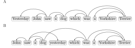
In the classic setting of Graph Theory, one aims to find an optimal embedding of a given graph, i.e. an embedding that yields or . In this context, research on and complements our understanding of the distribution of . Besides, and are of paramount importance in the context of the Theory of Spatial Networks, networks whose vertices are embedded in some space [12]. In this sort of networks, the layout is given by some random distribution as in Moon’s classic work [8, 9] or given by the physical position of every vertex of some real network [12]. Prototypical examples of the latter case are streets, roads and transportation networks (e.g., subway and train networks); these are spatial networks on a space that is usually assumed to be two-dimensional. The study of spatial networks is driven by development of that theory in non-Euclidean geometries [12]. However, the interest in networks whose vertices are embedded in a one-dimensional Euclidean space cannot be neglected. Remarkable examples are syntactic dependency networks and RNA structures. As for the former, the syntactic dependency network of a sentence can be defined as a network (usually a tree222Trees are undirected, connected, acyclic graphs.) where vertices are words, edges indicate syntactic dependencies, and their layout is a one-dimensional space where vertices are allocated in integer positions in and edges are drawn as semicircles above the sentence (Figure 1). Syntactic dependency structures have become the de facto standard to represent the syntactic structure of sentences in Computational Linguistics [13] and the fuel for many quantitative studies [14]. In that setup, edges may cross when drawn above the sentence (Figure 1). The one-dimensional layout of a syntactic dependency structure defines a linear arrangement of the vertices of the network, henceforth referred to simply as ‘linear arrangement’. Crossings may also occur in linear arrangements of RNA secondary structures, where vertices are nucleotides A, G, U, and C, and edges are Watson-Crick (A-U, G-C, U-G) base pairs [15]. A linear arrangement of a graph without crossings is called a one-page (book) embedding [16, 17] or a planar embedding [18].
The needs of computing the exact value of and efficiently are many. First, as a computational backup for mathematical research on the distribution of crossings in random layouts [8]. The algorithms presented here were crucial to find and correct some inaccuracies in Moon’s pioneering research [9]. Second, these two properties allow one to standardize real values of using a -score, defined as
| (2) |
-scores have been used to detect scale invariance in empirical curves [19, 20] or motifs in complex networks [21] (see [22] for a historical overview). Thus, -scores of would allow one to discover new statistical patterns involving in syntactic dependency trees, to name one example. Moreover, -scores of can help aggregate or compare values of from graphs with different structural properties (number of vertices, degree distribution,…), as it happens with syntactic dependency trees, when calculating the average number of crossings in collections of sentences of a given language [23]. Third, the crossing number is trivial when considering linear arrangements (‘la’) of trees: since trees are outerplanar graphs they admit a one-page book embedding [16], therefore, the minimum number of edge crossings that can be achieved in a linear arrangement of a tree is . Figure 1 illustrates two linear arrangements of the same tree.
However, other aspects of the distribution of are also very important, because random linear arrangements (henceforth denoted as ‘rla’) are used as baselines to answer many research questions. For instance, to check if the real number of in syntactic dependency structures is actually lower than expected by chance [23]. The large and growing collections of syntactic dependency structures that are available [25, 26] calls for efficient algorithms to calculate and . This can be applied to the improvement of tests for the significance of the real value of with respect to random linear arrangements which are based on a Monte Carlo estimation of the -value [23]. Using fast algorithms, an upper bound of the -value could be obtained immediately using Chebyshev-like inequalities, which require knowledge of and . If the -value was below the significance level, the null hypothesis could be rejected quickly, skipping the time-consuming estimation of an accurate enough -value.
Overview of previous work
On the positive side, the calculation of of a given graph is straightforward. It has been shown that
where is the probability that two independent edges cross in the given layout and is the size of the set of independent pairs of edges of the graph, denoted as , namely, the number of pairs of edges that do not share vertices [10]. can be computed in constant time given , the number of vertices of the networks, , its number of edges, , the second moment of degree about zero (i.e. the mean of squared vertex degrees) because
| (3) |
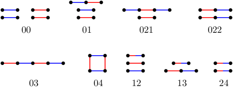
On the negative side, the calculation of is more complex [10]. Fortunately, its computation is a particular instance of a subgraph counting problem333 See [27, Chapter 4] for details on subgraph counting. [10]. The subgraphs to count in order to calculate are shown in Figure 2; a similar characterization can be found in [28, Figure 2] for trees whose vertices are in convex position444The vertices of a graph are in convex position when they are arranged in the boundary of a convex, closed, simple curve, assumed to be, without loss of generality, a circle.. Then, in an arbitrary graph becomes [10]
| (4) | ||||
is a layout-dependent term associated to type , defined later in Section 2 (Equation 11). is a set of subgraphs, where each is indexed by a code of two or three digits,
| (5) |
These codes were devised in [10]. In Equation 5, is an integer constant for each , and is the number of times the subgraph appears in the graph. Each is depicted in Figure 2; each of these graphs can be a connected graph or disjoint union of connected graphs. The values of , and are summarized in Table 1. In sum, is expressed as a function of the number of subgraphs of each kind that appear in Table 1. Notice that is the only graph-dependent term, and is the only layout-dependent term. The constant depends only on the type. The meaning of the codes listed in (Equation 5), which identify the graphs in Figure 2, is explained in Section 2.
| 0 | |||
| 2/9 | |||
| 1/18 | |||
| 1/45 | |||
| -1/9 | |||
| -1/36 | |||
| -1/90 | |||
| 1/180 | |||
| 0 |
Equation 4 can be seen as a particular case of the general equation to define a molecular property of a graph as a summation over all subgraphs , i.e. [29, 30]
where is the contribution of graph to the molecular property. In our case, we have that if is in Figure 2 and otherwise (in our case the summation is not restricted to connected subgraphs).
In this article, we aim to develop fast algorithms to calculate the exact value of in arbitrary graphs as well as ad hoc algorithms for forests. Forests are a straightforward generalization of trees which are the kind of graphs that are typically found in syntactic dependency structures. Moreover, notice that RNA secondary structures are graphs such that the maximum vertex degree is 1, thus a particular case of forests555It is worth mentioning that a formula of for 2-regular graphs was derived in [10].. In addition, the syntactic structures in recent experiments with deep agents are forests [31]. By providing algorithms for forests and, also, more general graphs, we are accommodating all the possible exceptions and variants that have been discussed to define the syntactic structure of sentences, e.g., allowing for cycles (see for instance, [32, Section 4.9 Graph-theoretic properties]).
Organization of the article
The remainder of the article has two parts. The first part develops gradually a formula for the variance by involving in the calculation the amount of certain subgraphs. Section 2 provides formal definitions, reviews the theoretical arguments in [10] which allows one to express as in Equation 4, and outlines a naive -time algorithm to calculate the exact value of that is based on subgraph counting. Section 3 builds on [10]: we first provide expressions to identify other, smaller subgraphs (Section 3.2) in the expansion of the expressions for all (Section 3.3). The expressions in Section 3.3 are obtained, essentially, by expanding the initial formal expressions in [10] and rearranging and regrouping the results. In Section 3.2 we also give expressions to easily count these new subgraphs in the algorithms devised in subsequent sections. We finish with Section 3.4 where we obtain a general arithmetic expression for via Equation 4 applying the expressions for all obtained in Section 3.3.
The second part is devoted to solving the counting problem algorithmically and is novel. In Section 4, we use the expressions in Section 3.4 to devise faster algorithms (Table 2). We present two algorithms that calculate for arbitrary graphs. Algorithm 4.2 runs in time and Algorithm 4.4 runs in time . We will show that the former is faster for sparse graphs and the latter is faster for dense graphs. Their time complexities are also given as a function of important graph structural parameters, such as the maximum vertex degree ; the second moment of degree about zero, which is an instantiation of the more general -th moment of degree about zero
| (6) |
where denotes the degree of vertex ; the sum of the product of degrees
| (7) |
the transitivity index [27, Chapter 4.5.1]
| (8) |
where is the number of subgraphs isomorphic to in ; and the degree of connectivity between pairs of vertices via a third vertex, denoted as an indicator function
| (9) |
We also present an algorithm for forests that runs in time (Algorithm 4.5).
Finally, Section 5 discusses our findings and their implications, and suggests future work.
Readers whose primary interest are the algorithms can jump directly to Section 4 after reading Section 2 (optional) and reading Sections 3.2 and 3.4 (mandatory). All the algorithms presented in this article were tested thoroughly (Appendix B) and are publicly available in the Linear Arrangement Library666Available online at: https://github.com/LAL-project/linear-arrangement-library [33].
| Algorithm | Time complexity | Space complexity |
|---|---|---|
| Naive algorithm | ||
| Algorithm 4.2 | ||
| (general graphs) | ||
| Algorithm 4.4 | ||
| (general graphs) | ||
| Algorithm 4.5 | ||
| (forests) |
2 Theoretical background
Consider a graph of vertices and edges whose vertices are arranged with a given function that indicates the position of every vertex in a given, fixed, layout. The number of crossings in , , can be defined by making explicit the dependence on a particular arrangement, as
where, recall, denotes the set of pairs of independent edges (i.e. the set of pairs of edges that may potentially cross [10], Equation 3), and where is an indicator function equal to if, and only if the edges and cross in the given arrangement embedded in the layout under consideration. Throughout this article we use . We omit from the notation when we denote a random variable. For example, hereafter we use to refer to for simplicity.
Next we review the steps devised in [10] towards Equation 4. By definition of a random variable’s variance,
Notice that
Let , which is the probability that any two independent edges cross in a given layout since is an indicator random variable, and, further, let and rewrite
Now we can express as
Expanding the square in the previous expression, can be decomposed into a sum of summands of the form , i.e.
| (10) |
The two elements of involved in the product can be classified into a type, which we denoted as , based on the relationship between the edges , , and . This classification system eventually leads to (Equation 5). This relationship was defined in [10] with two parameters:
-
•
, the number of common edges among , , and , and
-
•
, the number of common vertices among , , , , , , , and .
For example, consider the two elements of , and . In this example, there are no shared edges, ; but there are three common vertices, . Therefore, these two pairs are of type . It is depicted as a path graph of five vertices in Figure 2.
It is easy to see that there are only 9 types [10] of pairs of elements of . These are shown in Figure 2, where most are labeled using codes of two digits (the parameters and ) and only two types using three digits (the parameters and plus a disambiguation digit). The only two types that require a third digit are and since there are two possible graphs that can be made with such that and . We denote the set of all the types as (Equation 5). The features of each type of product are summarized in Table 3, which also includes the total number of distinct vertices in each type, denoted as .
Notice that, given any two , it is easy to see that
For the sake of brevity, let and when the pairs of independent edges can be classified into , i.e., when their type is one of the types in . Therefore,
| (11) |
For two fixed the value denotes the probability that in a uniformly random embedding (in the layout) of all the vertices of the edges , , , . Now, as a result of the classification described above, the expected values can be grouped into the different types in and thus can be expressed compactly as
| (12) |
where, for a fixed , is the number of occurrences of in the summation, defined as
| (13) |
Equation 13 is the formal definition of .
Notice, therefore, that computing can be done via countings of subgraphs. Figure 2 relates each type of product with the subgraph that has to be counted within the graph so as to obtain the exact value of . These graphs may be elementary graphs, a simple linear tree of a fixed number of vertices, e.g., or , a cycle graph, e.g., , or a combination with the operator , the disjoint union of graphs, all listed in Table 1.
In random linear arrangements (‘rla’), [10], and in uniformly random spherical arrangements (‘rsa’), [8]. In the latter layout, the vertices of the graph are placed on the surface of a sphere uniformly at random, and each edge of the graph becomes the geodesic between each of its corresponding vertices. It was shown that [10]
From these identities we can deduce that .
Table 3 gives all the values of and . These probabilities were calculated by brute force enumeration of all possible linear arrangements of the vertices of each type of graph.
| 00 | 8 | 0 | 0 | 1/9 | 0 | |
| 24 | 4 | 2 | 4 | 1/3 | 2/9 | |
| 13 | 5 | 1 | 3 | 1/6 | 1/18 | |
| 12 | 6 | 1 | 2 | 2/15 | 1/45 | |
| 04 | 4 | 0 | 4 | 0 | -1/9 | |
| 03 | 5 | 0 | 3 | 1/12 | -1/36 | |
| 021 | 6 | 0 | 2 | 1/10 | -1/90 | |
| 022 | 6 | 0 | 2 | 7/60 | 1/180 | |
| 01 | 7 | 0 | 1 | 1/9 | 0 |
Interestingly, is proportional to the amount of subgraphs of type , i.e.
| (14) |
where is an integer constant, and is the number of occurrences of the subgraph in the graph under consideration (Table 1).
Table 1 allows one to obtain via Equation 14. In [10], these expressions were used to obtain arithmetic expressions for in certain types of graphs, which were in turn used to obtain an arithmetic expression for in those classes of graphs, e.g., complete graphs, complete bipartite graphs, cycle graphs, etc. Such arithmetic expressions depend only on the number of vertices of the graph. In arbitrary graphs, we can still use Table 1 to derive a -time algorithm to calculate the exact value of . The naive algorithm is based on brute force enumeration of all elements of to count each . To do this, one can simply list all elements in and identify their respective types and count all the instances per type, namely, calculate . By doing this for all we can obtain all needed countings. This is formalized in Algorithm 2.1. Here we develop algorithms with lower asymptotic complexity for general graphs and forests. Table 2 summarizes the cost of the first approximations discussed here and that of the algorithms that are presented in subsequent sections.
3 Arithmetic expressions for
Here we further develop the algebraic expressions of the ’s for (Equation 5) but we focus on the ’s with non-null contribution to (Table 3). We use the formalization of the ’s in [10] as a starting point to obtain an arithmetic expression for in general graphs. These formalizations were originally used in [10] to obtain the expressions of the form of Equation 14.
The purpose of these algebraic expressions is to bridge the gap between the algorithms to calculate in Section 4 (Algorithms 4.2 and 4.5) and the countings over the set of subgraphs described in Section 2 (Equations 12 and 13).
In Section 3, we first describe the notation that we use in later sections to obtain compact expressions. In Section 3.2, we present general results that relate summations over the set with subgraph countings. These are used in Section 3.3, to obtain arithmetic expressions for . Finally, we derive an expression for in Section 3.4 using the .
3.1 Preliminaries
Throughout this article, we use letters to indicate distinct vertices. We define as the -th power of the adjacency matrix of the graph, where when , and if . Further, we define as the sum of one of half of the values of excluding the diagonal, i.e.
thus . We denote the sum of the degrees of the neighbors of a vertex as
| (15) |
The neighborhood intersection of two vertices and is denoted as
| (16) |
and the sum of the degrees of the vertices in as
| (17) |
Notice that if then . We also use (Equation 7) which is the sum of the product of degrees777Notice that this product is involved in the calculation of degree correlations [34]. at both ends of an edge. The values , , and prove useful in making the expressions of the ’s compact as well as in deriving the algorithms to compute the exact value of .
For any undirected simple graph , let be the induced graph resulting from removing vertex from . More generally, we define as the induced graph resulting from the removal of the vertices in . We use to refer to the set of pairs of independent edges of .


We denote simply as , illustrated in Figure 3(a). The number of edges in a graph is easy to calculate as a function of the number of edges in . If are four distinct vertices, then
| (18) |
Unless stated otherwise, network features refer to . Therefore, , , , … in Equation 18 refer to , and not to . We use to denote the set of neighbors of vertices in . Its size is:
| (19) |
We denote simply as , with . We use the term -path to refer to a sequence of pairwise distinct vertices such that . We consider and to be two different paths. Lastly, we use to denote the amount of subgraphs isomorphic to in .
The calculations of the ’s in subsequent sections require a clear notation that states the vertices shared between each pair of elements of for an arbitrary graph . Throughout this article we use summations of the form
where below each summation operand there is a scope on top of a condition. The “” represents any term. For the sake of brevity, we contract them as
Notice that the scope is omitted in the new notation. This detail is crucial for the countings performed with the help of these compact summations. Likewise, if we want to denote when two elements of from each of the summations share one or more vertices, we use:
This expression denotes the summation over the pairs of elements of in which the second one shares two vertices with the first one. Again, the expression to the left is a shorthand for the one to the right. For the sake of brevity, we also use two more compact summations:
3.2 General results
Here we introduce some results on summations over that we use in Section 3.3 to simplify expressions on the ’s; recall these were defined as summations over pairs of elements of (Equation 13). These expressions pave the way towards an efficient computation of , and hence of . The proof of each proposition can be found in Appendix A.
The results introduced here serve several purposes. One is to identify new subgraphs, which are , , , the paw graph (denoted as , Figure 4(a)), and (Figure 4(b)), involved in the counting of the types of graphs listed in Table 3 (shown in Figure 2). This first purpose is achieved by relating summations over elements of to counting these new subgraphs. The other purpose is to aid in the design of the algorithms in Section 4 to compute . These results are presented here to make the article more streamlined. We also present results involving summations of degrees of vertices of elements of . All of the results below are given for general graphs; some of them have been simplified for trees, since they can be generalized to forests quite easily.
The first three results involve .
Proposition 3.0.
The number of subgraphs isomorphic to , namely half the amount of -paths, in a graph is
| (20) | ||||
| (21) | ||||
| (22) |
Proposition 3.0.
Proposition 3.0.
In any tree ,
| (25) |
The next three results involve .
Proposition 3.0.
The number of subgraphs isomorphic to , namely half the amount of -paths, in a graph is
| (26) |
Proposition 3.0.
Proposition 3.0.

The next two propositions involve the paw graph and (Figure 4).
Proposition 3.0.
The number of subgraphs isomorphic to the paw graph (Figure 4(a)), denoted as , in a graph is
| (29) |
Proposition 3.0.
Proposition 3.0.
The number of subgraphs isomorphic to (Figure 4(b)) in a graph is
| (31) |
Proposition 3.0.
The next two propositions involve .
Proposition 3.0.
The number of cycles of vertices, namely , in a graph is
| (33) | ||||
| (34) |
Proposition 3.0.
There are other useful results regarding the sum of the degrees of all vertices involved in the elements in .
Proposition 3.0.
Furthermore, we identify products of degrees of vertices that appear in the following derivations. These are useful to obtain the formula for and to compute them in an algorithm.
Proposition 3.0.
Proposition 3.0.
Finally, we define two new values which are found throughout coming derivations. These two are needed in Sections 3.3.5 and 3.3.6 to obtain a formula for . First, let
| (39) |
and let
| (40) |
The following results ease the computation of and .
Proposition 3.0.
Proposition 3.0.
Sections 3.2 and 3.2 can be further refined for the special case of trees.
Proposition 3.0.
Proposition 3.0.
3.3 Formulas for the frequencies
In the following subsections, we obtain general expressions for the ’s based on the formalization given in [10] and Sections 3.2, 3.2, 3.2, 3.2, 3.2, 3.2, 3.2 and 3.2. These expressions are designed based on three non-exclusive principles: easing the computation of , linking with standard Graph Theory and linking with the recently emerging subfield of crossing theory for linear arrangements ([10, Section 2] and also [28, 35]). In [10], the expressions for the ’s were linked with Graph Theory via (recall Section 2)
In the coming subsections, we derive simpler arithmetic expressions for the ’s to help derive arithmetic expression for (Section 3.4). We focus on the ’s that actually contribute to , namely those such that because [10]. An overview of the expressions that are derived for the ’s is shown in Table 4.
| Equation | |
|---|---|
| 45 | |
| 48 | |
| 51 | |
| 3.3.4 | |
| 56 | |
| 65 | |
| 67 |
Our approach consists of further developing the algebraic formalizations of the given in [10], which are briefly summarized below in this article to make it more self-contained. In Appendix B, we explain the tests employed to ensure the correctness of said expressions. When reading the sections to come, we suggest the reader to recall the definition of and in Section 2.
3.3.1 ,
It was already shown in [10] that
| (45) |
3.3.2 ,
This type denotes the pairs of edges sharing exactly one edge () and that have 3 vertices in common (). It was shown in [10] that
| (46) | ||||
| (47) |
See Figure 3(b) for an illustration of the first inner summation in Equation 46. Now we simplify Equation 47. Since implies we obtain
Finally, Sections 3.2 and 3.2 allow one to rewrite as
| (48) |
3.3.3 ,
was formalized as [10]
| (49) | ||||
| (50) |
Figure 3(c) illustrates Equation 49. Using Equation 18, we rewrite as
which, thanks to Sections 3.2 and 3.2, leads to
| (51) |
3.3.4 ,
All pairs of elements of classified into this type share no edges yet have 4 vertices in common. This allowed a brief formalization for in [10]
| (52) |
Therefore, by Section 3.2 we rewrite Equation 52 as
| (53) |
3.3.5 ,
was formalized as [10]
| (54) |
where , , … are functions over . In particular these are defined as
| (55) |
where are explicit distinct parameters and as implicit parameter. Examining separately, we see that, given , counts the amount of neighbors of in if , counts the amount of neighbors of in if , and so on. Figure 3(d) illustrates .
Here we obtain a simpler expression for Equation 54 by simplifying first the inner sum of all the . For this, we apply Equation 19 to a pairwise sum of these so as to obtain a series of expressions that are easier to evaluate
When adding all of them together, we can simplify the expression a bit more
Upon expansion of the positive part of the expression, we obtain
and, upon expansion of the negative part,
Thanks to the results for each part, the expression for becomes
By noticing that, via a simple rearrangement of the terms inside the summation,
where is defined in Equation 39, and thanks to Sections 3.2, 3.2 and 3.2, can be simplified further,
| (56) |
3.3.6 , , Subtype 1

(Figure 5) can be formalized as
| (57) |
where [10]
| (58) | ||||
| (59) |
and and are functions over , being the explicit parameters and as implicit parameters. These functions are defined as
| (60) | |||||
| (61) | |||||
for .
The functions and count the elements of the form of the illustrated in Figures 3(e), 5(a) and 5(d). The first function counts, for each neighbor of , say , the number of neighbors of , say , such that . Likewise for the second function. On the other hand, the values , , , count the edges , such that when paired with , , , form an element of whose form is that of those elements illustrated in Figures 3(f), 5(b) and 5(c). These amounts are counted only if such edges exist in the graph, hence the factor for , and likewise for the other .
Recall that for , . Then, thanks to Sections 3.2 and 3.2, we obtain
On the other hand, Equation 19 leads to
| (62) |
Likewise for
| (63) |
The negative summations in , Section 3.3.6 (and , Equation 63) represent the amount of vertices from neighbors of (of ) in that are also neighbors of (of ), in , i.e., the triangles formed by vertices and respectively. Then, Equation 58 becomes
Within ,
| (64) |
and, within ,
Then Equation 39, and Sections 3.2, 3.2 and 3.2 allow one to rewrite Equation 57 as
| (65) |
where is defined in Equation 37.
3.3.7 , , Subtype 2
(Figure 6) was formalized as [10]
| (66) |
where is an auxiliary function defined as in Equation 60. can be understood from the case of in Figure 3(e).

We now derive a useful arithmetic expression for . First, we expand, following Sections 3.3.6 and 63, the in Equation 66 as
Inserting these expressions into Equation 66 and taking common factors out, one obtains
which can be further developed and then simplified using Sections 3.2, 3.2 and 40, becoming
Using Propositions 3.0 and 3.3.6, Sections 3.2 and 3.2, and by expanding , we finally obtain
| (67) |
3.4 Variance of the number of crossings
Applying the arithmetic expressions of the ’s above (summarized in Table 4) to Equation 4, we obtain
| (68) |
where is the number of pairs of independent edges (Equation 3), is defined in Equation 36, and are defined in Equations 37 and 3.0, and are defined in Equations 39 and 40, and is the graph paw and , depicted in Figure 4. Since forests are acyclic, , and then the variance of becomes
| (69) |
For the case of uniformly random linear arrangements, the instantiation of Section 3.4 gives
| (70) |
and the result of instantiating Section 3.4 is
We refer the reader to [10, Table 5] for a summary of expressions of in particular classes of graphs (complete graphs, complete bipartite graphs, linear trees, cycle graphs, one-regular, star graphs and quasi-star graphs).
4 Algorithms to compute
In this section we provide algorithms that compute the exact value of in general graphs (based on Section 3.4) in Section 4.1 and in forests (based on Section 3.4) in Section 4.2. Since the computation of reduces to a subgraph counting problem (as seen in previous sections), the algorithms presented below consist of solving the subgraph counting problem that we face in Sections 3.4 and 3.4 and then calculating with knowledge of . The subgraph counting problem was presented in Section 3.2.
4.1 An algorithm for general graphs
Our algorithm to calculate is a simple traversal of the edges of the graph with some extra work to be done for each edge, which is, basically, a traversal over the neighborhood of the endpoints. For general graphs, this yields an algorithm of time complexity .
This algorithm was derived combining three strategies. First, we have shown that the values , , and are linear-time computable in or since they have very simple arithmetic expressions (see Equations 3, 36, 37 and 3.0, respectively). Second, the subgraphs present in Section 3.4, namely , , , and (the last two are depicted in Figure 4) could be counted straightforwardly by relying on previous work [36, 37]. For example, we could use Alon et al.’s contributions [36] on the counting of and in graphs, and Movarraei’s contributions [37] regarding formulas to count all instances of and in graphs. However, these methods require using the adjacency matrix of the graph and we have opted for a combinatorial approach that does not employ it; we discuss this in deeper detail in Sections 5.2 and 5.3. Third, we apply the reinterpretation of and (in Equations 41 and 42) which states that their value can be computed without enumerating the elements of .
All the expressions in Section 3.2 are integrated in Algorithm 4.2 to compute the exact value of in a straightforward manner. We formalize the complexity of this algorithm in Section 4.1.
Proposition 4.0.
Let be a graph with and . Let the graph be implemented with sorted adjacency lists, namely, the adjacency list of each vertex contains labels sorted in increasing lexicographic order. Algorithm 4.2 computes in in time and space .
Proof.
The computation of ’s value is done by putting together all the results presented in this work that involve the terms in Section 3.4. The results’ correctness has already been proved and the algorithm uses them in a straightforward manner. The space complexity is easy to calculate: we need -space to store the values of the function (Equation 15) for each vertex .
As for the time complexity, the cost of Setup (Algorithm 4.1) is and then the algorithm iterates over the set of edges and performs, for each edge, three intersection operations to compute the values , and . The other computations are constant-time operations as a function of the vertices of similar intersection or as a function of the vertices of the edge. Now, if we denote the cost of the intersection of two sorted lists and as , the algorithm has cost
It is easy to make an algorithm to calculate the intersection of two sorted lists with cost . This leads to the following cost function
Obviously, the first summation is (Equation 7) and the second summation equals . The third summation is also easy,
Therefore, the algorithm has time complexity
We can easily derive an upper bound of the cost which, although generous, gives a more understandable cost of the algorithm. Simply, notice that
The algorithm’s cost is now expressed in terms of and the structure of the graph, as captured by . To obtain a cost in terms of and , we use which follows from the fact that (Equation 3); and thus the cost can be expressed as . ∎
Notice that the assumption that the graph’s adjacency list being sorted merely simplifies the algorithm. In case it was not, sorting it, prior to the algorithm’s execution, has cost when using a comparison-based algorithm. Algorithms that are not based on comparisons may have lower time complexity. For instance, counting sort [38] can sort numbers in time and space if their values range within the interval . In an adjacency list, the entry corresponding to vertex contains values which range within the interval ; sorting can be done in space , and time .
In Section 4.1.1 we extend Algorithm 4.2 to reuse computations and show, using empirical results, that doing so produces an algorithm several times faster in practice.
4.1.1 Improving the algorithm by reusing computations
Here we improve Algorithm 4.2 by reusing the computations that are marked in red. The new algorithm is detailed in Algorithm 4.4 and its complexity is analyzed in Section 4.1.1, where we show that the transitivity index of a graph (Equation 8) influences its space complexity.
Algorithm 4.4 reuses the calculation of the number of common neighbors of two not-necessarily-adjacent vertices , , i.e., , defined in Equation 16, and the sum of the degrees of the vertices that are neighbors of both vertices , defined in Equation 17. These values are marked in red in Algorithm 4.2. In order to reuse them, Algorithm 4.4 makes use of a hash table whose keys are unordered pairs of vertices and , denoted as , and the associated values are and . Keys are made up of vertices that are either adjacent () or there exists another vertex such that . Notice that these cases are not mutually exclusive: if two vertices are both adjacent and connected via a third vertex (i.e., when and are vertices of a ) then the values associated are computed only once and the pair is stored only once. The same applies if and are not adjacent but are connected via another vertex (and then and are the ends of some ).
Whenever or are needed, the pair is first searched in . If has such pair, its associated values are retrieved. If it does not, both and are computed and stored in . This update step is detailed in Algorithm 4.3. These ideas yield Algorithm 4.4, where changes with respect to Algorithm 4.2 are marked in red.
To better analyze the cost of the algorithm, we use as defined in Equation 9.
Proposition 4.0.
Consider a graph that is implemented as in Section 4.1. Algorithm 4.4 computes of in time
and space complexity , where is the size of the hash table at the end of the algorithm
| (71) |
where is the transitivity index of a graph (Equation 8).
Proof.
The space complexity of this algorithm depends on the memory used to store the values of function (Equation 15) and the size of the hash table at the end of its execution. The former needs -space. Now follows a derivation of ’s size.
Recall that the size of any hash table is proportional to the amount of keys plus the values associated to each of them. In our case, the keys have fixed size (a pair of vertices) and the amount of values associated to the keys is always constant (two integers), so we only need to know the amount of keys it contains at the end of the algorithm.
As explained above, pairs of vertices are added to in two not necessarily mutually exclusive cases. When (1) the vertices are an edge of the graph (), and when (2) the two vertices are connected via a third vertex (). Since the second event includes the first, we simplify (2) to the case when and . Define as the amount of pairs in (1), and as the amount of pairs added in (2). Then, .
The first case is easy: . Consider now case (2). In this case, and are the vertices of an open (if and were adjacent then the would be closed, also a ). The exact value of is the amount of pairs of vertices , such that and ,
An upper bound of is the number of open in a graph, i.e.,
The size of can be expressed in two different ways. First, easily enough, we can express the size of using the transitivity index
| (72) |
In the worst case, . For example, in a complete graph . Second, since [39, p. 103]
| (73) |
we get that
Applying Equation 73 to Equation 72, we obtain via straightforward arithmetic operations the cost in Equation 71.
Its time complexity is given by the amount of work to be done for each pair of vertices to be passed as an argument of Algorithm 4.3 in Algorithm 4.4 (Algorithms 4.4, 4.4 and 4.4). Let be the number of times the pair is passed as an argument of a call to Algorithm 4.3. It is easy to see that . For every such pair, the algorithm performs an intersection operation of cost once, and exactly operations of constant-time cost.
The total running time assuming that is then
where is the cost of Algorithm 4.1. We will bound the second term by parts. First notice that
where denotes the set of all unordered pairs of different vertices of . Second, notice that
where, since ,
The total time complexity of reusing computations is, then,
∎
4.1.2 Analysis in Erdős-Rényi random graphs
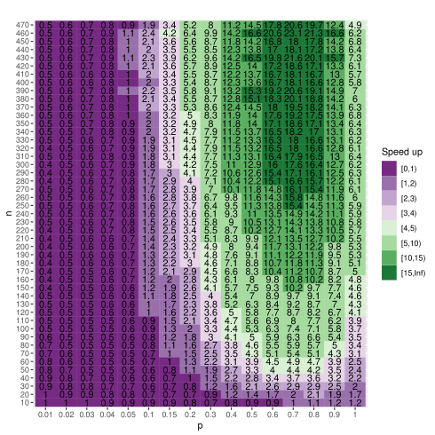
Comparing the running time of Algorithm 4.2 and Algorithm 4.4, it is easy to see that the latter reduces the asymptotic upper bound of the time cost (Table 2), suggesting that it should be faster in denser graphs. However, this does not imply that Algorithm 4.4 is faster in general: the time costs are asymptotic estimates of upper bounds. Therefore, we evaluate the potential speed-up of Algorithm 4.4 with the help of Erdős-Rényi random graphs [40, Section V]. Figure 7 shows that reusing computations (Algorithm 4.4) is faster for sufficiently dense -vertex graphs, given a fixed . Both algorithms are available in the Linear Arrangement Library [33]888We used 2017–C++ standard. The hash table was implemented using the template class std::unordered_map, in which insertions and lookups have constant-time complexity. We used GNU’s gcc compiler, version 11.1, and we used the usual optimization flags, such as -O3. The hashing scheme we used can be found in the implementation of an R package for cluster analytics [41]. Execution time was measured on an Intel Core i5-10600 CPU 3.30 GHz..
It is easy to see from Figure 7 that the speed up depends on both and . To prove this we give the expected running time of both algorithms in . We start with Algorithm 4.2.
Proposition 4.0.
The expected running time of Algorithm 4.2 in a graph is
Proof.
Recall the cost of the algorithm in Section 4.1. First, it is well known that . Second,
We obtained the value by applying the Total Law of Expectation
and
as . Lastly,
since [42]. ∎
Before we derive the expected time and space complexities of Algorithm 4.4 in Erdős-Rényi graphs, we first present an intermediate result.
Lemma 4.1.
Consider a graph . For any two we have that
Proof.
The proof is straightforward
∎
We continue with Algorithm 4.4.
Proposition 4.1.
The expected running time of Algorithm 4.4 in a graph is
Proof.
We calculate the expected running time from its asymptotic cost in Section 4.1.1.
As is an indicator variable,
The value of is given in Lemma 4.1. The expected asymptotic cost now follows from straightforward calculations. ∎
We still cannot calculate the theoretical speedup of reusing computations in graphs that follow the Erdős-Rényi random graph model since the expected costs obtained are approximate upper bounds of the actual cost. Their quotient, therefore, gives us an approximate lower bound of the speed up of reusing computations. The speed-up of reusing computations is then . Put differently, the boundary of the region where reusing computations is warranted to be faster is given by for some constant . Besides, the empirical analysis of the actual speed up of reusing computations in Figure 7 shows two regions: one where reusing computations is slower and another where reusing computations is faster. Interestingly, the boundary between regions (the points in Figure 7 where the speed up is one) is defined by a curve that decreases as increases (for small ), consistently with the approximate theoretical analysis.
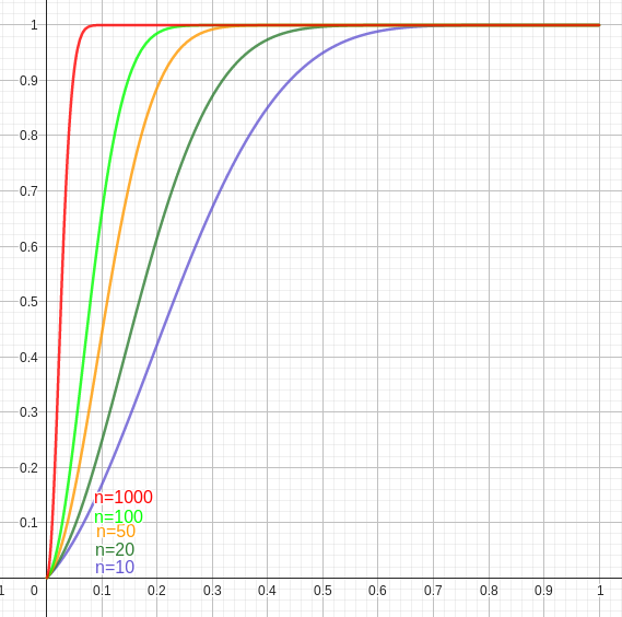
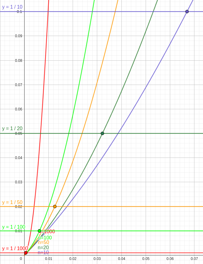
Finally, we also analyze the expected size of in Erdős-Rényi. Section 4.1.2 shows that the probability that a pair of vertices is in grows quickly to 1 for sufficiently large , indeed the effect is sharper as increases. Consequently, the expected size grows as increases but reaches , its maximum value, quickly for sufficiently large .
Proposition 4.1.
Consider Algorithm 4.4 on a graph . Let be an indicator random variable that equals when is in and 0 otherwise. Then the probability that a is in is
| (74) |
and the expected size of at the end of the algorithm is then
| (75) |
Proof.
Figure 8 shows the growth of the probability function in Equation 74, , for several values of . It can be seen that the probability of any pair of two vertices to be in at the end of the algorithm surges with and reaches values close to rapidly, even for low . Therefore, in Erdős-Rényi graphs, the function in Equation 75 reaches at the same rate as reaches .
It is worth studying at what values of we should expect to have size as this is the size cost of Algorithm Algorithm 4.2. These are the values of for which , for some constant . There does not seem to be an exact solution, but we can easily derive an upper bound that indicates that these values vanish as increases.
Proposition 4.1.
Consider a graph . The value of such that the expected size of at the end of Algorithm 4.4 is , satisfies
Proof.
We start by rearranging terms and applying logarithms
Notice that
and
from which we can obtain the desired result. ∎
Figure 9 shows the points , where is the probability in for which (Equation 74) equals .
4.2 An algorithm for trees and forests
When instantiating Algorithm 4.4 on forests, its time complexity can be easily estimated to be , and its space complexity to be (since for any forest ). However, can be computed in time and space in forests by exploiting their acyclicity. We first draw the attention of the reader to the simplified subgraph counting formulas for , given in Section 3.2 (Sections 3.2 and 3.2). We draw the attention of the reader to the simplification of and (Equations 39 and 40) in Section 3.2 (Sections 3.2 and 3.2). We prove the algorithm’s correctness and complexity in Section 4.2.
Proposition 4.1.
Let be a forest of vertices. Algorithm 4.5 computes in in time and space .
Proof.
The terms , , and are defined for general graphs as sums of values that only depend on vertices that are adjacent (Equations 3, 36, 37 and 3.0). The terms and , and can be computed in forests as easily as they can be computed in trees. Namely, the arguments in the proofs of Sections 3.2, 3.2, 3.2 and 3.2 that led to their respective equations can be extended to forests straightforwardly while keeping the same conclusions thanks to the fact that forests, as their definition states, are merely a disjoint union of trees.
Recall that in a forest with connected components. Then, it is easy to see that the time complexity of the algorithm is since the loop in Algorithm 4.5 iterates over the set of edges of , and the computation of the is also done in steps. It is also obvious that the space complexity is since we have to store the values of for each . ∎
5 Discussion and future work
We start discussing the primary goal of this article, namely the problem of computing efficiently (Section 5.1). Then, since the calculation of reduces to a problem of counting the number of subgraphs of a certain type (Equation 4 and Table 1), we proceed to discuss our contributions with respect to two research problems that are by-products of our primary goal: the counting of all subgraphs (Section 5.2) and the counting of specific subgraphs (Section 5.3). Indeed, the problem of the computation of can be seen as an instance of a third research problem: counting on a prescribed set of subgraphs. We conclude suggesting future research (Section 5.4).
5.1 Computation of variance
We have developed efficient algorithms to calculate in general graphs and also in forests. Part of our work consists of reducing the complexity of the computation of arithmetic expressions of the ’s for all types (except types and , since ). Using Section 3.4, we derived algorithms tailored to layouts meeting the requirements characterized in Section 1.
We have alleviated the complexity of the computation of for such layouts by several orders of magnitude (Algorithm 4.2) with respect to the naive -time subgraph counting algorithm introduced in Section 2. Moreover, we have also improved Algorithm 4.2 to reuse computations (Algorithm 4.4) and tailored a solution for forests that is even faster than a direct instantiation of Algorithm 4.4.
Furthermore, we have demonstrated the advantage of reusing computations on Erdős-Rényi random graphs theoretically and measured empirically the speed up of reusing computations in Erdős-Rényi random graphs. Figure 7 shows significant speed up values in dense graphs. However, reusing computations introduces a non-negligible cost in very sparse graphs: Algorithm 4.2 seems to be faster than Algorithm 4.4 for low of () and . Nevertheless, it is important to notice that the speed up measurements in sparse graphs seem to have an increasing (though slow) tendency, which suggests that reusing computations in sparse graphs is favorable when is large ().
5.2 Counting subgraphs in general
Since the calculation of reduces to a problem of counting the number of subgraphs of a certain type (Equation 4 and Table 1), one could also apply algorithms for counting graphlets or graphettes [44, 45]. Graphlets are connected subgraphs while graphettes are a generalization of graphlets to potentially disconnected subgraphs. The subgraphs for calculating the number of products of each types are indeed graphettes; only types 03 and 04 the subgraphs are graphlets (Figure 2). As the subgraphs we are interested in have between 4 and 6 vertices999Recall that types and do not matter. (Figure 2), we could generate all subsets of 4, 5 and 6 vertices and use the look-up table provided in [45] to classify the corresponding subgraphs in constant time for each subset. However, that would produce and algorithm that runs in time while ours runs in if we do not reuse computations and in if we reuse them (Table 2).
5.3 Counting specific subgraphs
Our algorithms are based on formulas for the ’s, namely, the number of products of each type (Table 4). As a side-effect of such characterization, we have contributed with expressions for the number of paths of 4 and 5 vertices of a graph (Sections 3.2 and 3.2) that are more compact than others obtained in previous work [37].
The subgraphs present in Section 3.4, namely , , , and (the last two are depicted in Figure 4) could be counted easily by relying on previous work by Alon et al. [36] and Movarraei [37] based on powers of the adjacency matrix. For example, Alon et al. [36], among many other contributions, showed that
Moreover, Movarraei [37] showed that
It easy to see that the expressions by Alon et al. and those of Movarraei can all be computed in time , where is the exponent of the fastest algorithm for matrix-matrix multiplication, as already pointed out by Alon et al. [36, Theorem 6.3]. The value of depends on the algorithm used (obviously, ). The starting point is Strassen’s, with [46]. This cost can only be lowered by applying improvements of increasing complexity over already-complex algorithms (such as Strassen’s [47], Coppersmith-Winograd’s [48, 49]) which may introduce large constants that multiply execution time [50]. Moreover, some algorithms may need to enlarge the matrices to operate properly101010For example, Strassen’s algorithm requires the number of rows (and of columns) to be a power of in the matrices being multiplied [46]. This can be achieved by padding the matrix with ’s, but it may become infeasible quite quickly..
Now, in this paper we followed an alternative approach, combinatorial in nature, to reduce the time and space complexities with respect to the naive algorithm (Algorithm 2.1), in which we developed and applied supporting expressions to count many distinct subgraphs. It is clear that the complexity of this approach is determined by the complexity of the more complex subgraphs to count, namely, and . Our main goal was to devise an algorithm whose time complexity adapted to the graph’s structure.
The first algorithm we devised (Algorithm 4.2) has time complexity and space complexity (Section 4.1). Although there is some compensation as far as space complexity is concerned, its complexity is obviously much higher than that of a naive matrix-matrix multiplication algorithm. We developed a second algorithm (Algorithm 4.4) to reduce time complexity at the expense of space complexity; Algorithm 4.4 has time complexity and space complexity (Section 4.1.1). While the space complexity of this algorithm is asymptotically the same as using adjacency matrices, it is, in the worst case, as fast as that of a naive matrix-matrix multiplication algorithm. We can conclude, therefore, that, when compared to an algorithm that uses adjacency matrices, Algorithm 4.4 has the same drawbacks as far as space complexity is concerned, but it has advantages concerning time complexity since it is adaptive to the graph’s structure.
5.4 Future work
Concerning the algorithms and their underlying theory, future work should investigate simpler formulas for the number of products of the types, specially types that are relevant for the calculation of variance but for whom a simple arithmetic formula is not forthcoming yet, i.e. types 03, 021 and 022 (Table 4). In this and previous articles [42], we have provided a satisfactory solution to the computation of the first and the second moments of about zero, i.e. and . Similar methods could be applied to derive algorithms for higher moments, e.g., .
Concerning applications, the algorithms above pave the way for many applications. A crucial one is offering computational support for theoretical research on the distribution of crossings in random layouts of vertices [8, 9]. In the domain of statistical research on crossings in syntactic dependency trees [23], has been shown to be significantly low with respect to random linear arrangements with the help of Monte Carlo statistical tests in syntactic dependency structures [23]. Faster algorithms for such a test could be developed with the help of Chebyshev-like inequalities that allow one to calculate upper bounds of the real -values. These inequalities typically imply the calculation of , which is straightforward (simply, [10]) and the calculation of , that thanks to the present article, has become simpler to compute. Similar tests could be applied to determine if the number of crossings in RNA structures [15] is lower or greater than that expected by chance. For the same reasons, our algorithms allow one to calculate -scores of (Equation 2) efficiently. -scores have been used to detect scale invariance in empirical curves [19, 20] or motifs in complex networks [21] (see [22] for a historical overview). Thus, -scores of could lead to the discovery of new statistical patterns involving . Moreover, -scores of can help aggregate or compare values of from graphs with different structural properties (number of vertices, degree distribution,…). In addition, -scores of can help to aggregate or compare values of from heterogeneous sources as it happens in the context syntactic dependency trees, where one has to aggregate or compare values of of syntactic dependency trees from the same language but that differ in parameters such as size or internal structure (e.g., different value of ) [23]. We hope that our algorithms stimulate further theoretical research on the distribution of crossing as well as research on crossings in spatial network, specially in the domain of linguistic and biological sequences.
Acknowledgments
We are grateful to J. L. Esteban for helpful comments. LAP is supported by Secretaria d’Universitats i Recerca de la Generalitat de Catalunya and the Social European Fund. This research was supported by the grant TIN2017-89244-R from MINECO (Ministerio de Economía y Competitividad) and the recognition 2017SGR-856 (MACDA) from AGAUR (Generalitat de Catalunya). The authors are currently supported by a recognition 2021SGR-Cat (01266 LQMC) from AGAUR (Generalitat de Catalunya).
Declarations
Conflict of interest
The authors declare that they have no conflict of interest.
Appendix A Proofs
Here we give the proofs of many of the propositions given throughout this work. In particular, we give the proofs of those non-trivial propositions that are relevant enough regarding the goal of this paper.
A.1 Proof of Section 3.2
Let be a pair of edges from . It is easy to see that the expression counts how many we can make with these two edges. By definition of , . To these two edges, we only have to add one of the four edges in the expression (i.e., any of the edges that connect a vertex of with another vertex of ) to make a . Each of the edges in the expression produces a distinct (Figure 10).

Let be the set of into which is mapped. The of follow a concrete pattern: the edges of are at each end of the (Figure 10). Equation 20 could be false for two reasons. Firstly, some is not counted. Suppose that there exists a with vertices in that is not counted in the summation. If this was true then the pair of independent edges we can make using its vertices () would not be in . But this cannot happen by definition of . Secondly, some is counted more than once. It can only happen when there exists a such that . For this to happen, must place the same edges as at the end of the , which is a contradiction because . Therefore, such a does not exist.
A.2 Proof of Section 3.2
Consider three vertices ,, inducing a path of vertices in : . We can count all induced subgraphs that start with vertices and finish at by counting how many are different from and in the neighborhood of , . Then,
We replace the inner-most summation with the expression . This expression, when summed over the vertices , can be simplified further leading to
It is easy to see that
Obtaining the expression in Equation 23 is now straightforward.
A.3 Proof of Section 3.2
The proof is similar to the proof of Section 3.2. For a given , the inner summations of Equation 26, i.e.
count the number of we can make with edges and of . This set of is denoted as and contains the that follow a concrete pattern: each edge of is at one end of the and the edges of are linked via a fifth vertex , such that (Figure 11). For example, may contain if . Therefore, the graphs , for any , have different forms determined by the choice of the vertex of each edge of that will be at one of the ends of the .

Similarly, Equation 26 could be wrong for two reasons: some path may be counted more than once or not counted at all.
All are counted: by contradiction, given , suppose that there is a , , not counted in the inner summation. By definition of , , the vertices are distinct and we have . Therefore, if such is not counted then would not be in .
Some may be counted more than once: if this was true then for some there would exist a , , such that . For this to happen, must place the same edges as at the end of the , which is a contradiction because . Therefore, such a does not exist.
As a conclusion, all paths are counted, and no path is counted more than once. Therefore, Equation 26 evaluates to exactly all in .
A.4 Proof of Section 3.2
The proof is similar to the proof of Section 3.2.
A.5 Proof of Section 3.2
Any has only one centroidal vertex . For any pair of different neighbors of , and , the product gives the amount of with centroidal vertex and through vertices and . Therefore
| (76) |
Notice that the two inner summations of Equation 76 count such paths, twice. As
we finally obtain
with .
A.6 Proof of Section 3.2
The proof is similar to that of Section 3.2. We first show that the term in the summation
counts the amount of subgraphs isomorphic to in that we can form given . This can be easily seen in Figure 12 where, for a given , are shown all possible labeled graphs, , isomorphic to , that can be made with and assuming the existence of the pairs of edges in the summation . This means that when counting how many of these pairs of adjacencies exist we are actually counting how many subgraphs isomorphic to exist that have these four vertices.

Now we prove the claim in this proposition by contradiction. Since we know that the term inside the summation counts all labeled that can be made with every element of , the claim can only be false for two reasons: in the whole summation of Equation 29 some is not counted, and/or some of these is counted more than once.
Firstly, it is clear that all are counted at least once. If one was not counted then the element of we can make with its vertices would not be in which cannot happen by definition of .
Secondly, none is counted more than once. Let be the set of labeled graphs is mapped to. A paw is a triangle with a link attached to it. The paws in follow a concrete pattern: is linked to a triangle containing , or the other way around, is linked to a triangle containing (Figure 12). If any is counted twice then there exists a different such that . For this to happen, must place the same edges as in and outside the triangle of the paw, which is a contradiction because . Therefore, such a does not exist.
A.7 Proof of Section 3.2
We use for brevity. Similarly as in previous proofs we first show that the inner summation of the right hand side of Equation 31, i.e.,
| (77) |
counts the amount of graphs isomorphic to that can be made using the edges of , which we denote as . Graphs in follow a concrete pattern: if edge is part of then is the , and vice versa. The is completed with another vertex neighbor to the other two vertices of the . None of the graphs in are repeated and are illustrated in Figure 13.

Let be the set of vertices of a where the and . Then we have that . If a was not counted in Equation 31 it would mean that none of these elements would be in . This cannot happen by definition of . Finally, since we can make three elements of from , every is present in the set of three different . Hence the factor in Equation 31.
A.8 Proof of Section 3.2
The first equality was proven in [10, section 4.4.5]. Equations 33 and 34 follow from previous results in [36, 51]. Suppose that is the number of different cycles of length 4 that are contained in [36]. More technically, is the number of subgraphs of that are isomorphic to .
We have that [36]
| (78) |
with
A similar formula for was derived in the pioneering research by Harary and Manvel [51]. The fact that and [36], transforms Equation 78 into Equation 33. Recalling the definition of in [52]
we may write equivalently as
A.9 Proof of Section 3.2
The amount of edges of the graph induced from the removal of vertices and
| (79) |
The proof is straightforward. First,
Thanks to Equation 79 one obtains
where is defined in Equation 7.
A.10 Proof of Section 3.2
A.11 Proof of Section 3.2
The proof is also straightforward. We start by noticing that
For a fixed edge , the inner summation above sums over the set
Then, for a fixed edge , this leads to
A.12 Proof of Section 3.2
First, take notice that whenever one of the adjacencies , , or equals , the summation in Equation 39 adds the degree of the first and last vertices of the induced by the edges , and the adjacencies that equal . Therefore, it is easy to see that
where is defined in Equation 17.
A.13 Proof of Section 3.2
Similarly as in Section 3.2, we can see that the summation in Equation 40 adds the degrees of the vertices of each in . Therefore, we can express Equation 40 equivalently as
Appendix B Testing protocol
The derivations of the ’s in Section 3.3 and the algorithms to compute presented in Section 4 have been tested thoroughly via automated tests. For these algorithms we only consider the case of uniformly random linear arrangements, i.e., . Here we detail how we assessed the correctness of the work presented above.
The calculation of the ’s have been tested comparing three different but equivalent procedures whose results must coincide. Firstly, the ’s are computed by classifying all elements of into their corresponding (Table 3 for the classification criteria). Secondly, the ’s are computed via Equation 14 after counting by brute force the amount of subgraphs corresponding to each (Figure 2). Finally, the ’s are calculated using the expressions summarized in Table 4 with a direct implementation of the corresponding arithmetic expression. Such a three-way test was performed on Erdős-Rényi random graphs [40, Section V] of several sizes () and three different probabilities of edge creation . The test was also formed on particular types of graphs for which formulas for the ’s that depend only on are known: cycle graphs, linear trees, complete graphs, complete bipartite graphs, star trees and quasi star trees [10], for values of .
The algorithms in Section 4 have been tested in three ensembles of graphs: general graphs, forest and trees. The values of are always represented as an exact rational value (the GMP library (see https://gmplib.org/) provides implementations of these numbers). In each ensemble, is computed in a certain number of different ways. The test consists of checking that all the ways give the same result. The first way, , consists of computing by brute force, i.e., by classifying all elements in to compute the values of the ’s that are in turn used to obtain via Equation 4. The second way, , is obtained computing with a direct implementation of the derivations of the ’s (summarized in Table 4). , is obtained computing via Algorithm 4.2. Finally, we also computed in forests using Algorithm 4.5, denoted as , and in trees, denoted as . Within in each ensemble of graphs, the details of the test are as follows:
-
1.
General graphs. In this group we computed for for all the following graphs: Erdős-Rényi graphs (for and ), complete graphs (), complete bipartite graphs (all pairs of sizes with ), linear trees (), one-regular graphs (all even values of ), quasi-star trees (), star trees () and cycle graphs (). Since the computation of is extremely time-consuming in dense Erdős-Rényi graphs with a high number of vertices (, ), we computed it once for all these graphs and stored it on disk.
-
2.
Forests. In this group we computed for in all the trees listed above and also in forests of random trees. We generated these forests by joining several trees of potentially different sizes generated uniformly at random. The total size of the forest was always kept under .
-
3.
Trees. In this group we computed for , in all free unlabeled trees of size .
References
- \bibcommenthead
- Schaefer [2017] Schaefer, M.: The graph crossing number and its variants: a survey. The electronic journal of combinatorics, 21 (2017)
- Buchheim et al. [2013] Buchheim, C., Chimani, M., Gutwenger, C., Dortmund, T.U., Jünger, M., Mutzel, P.: Crossings and Planarization. Handbook of Graph Drawing and Visualization, pp. 56–100. CRC press, Boca Raton (2013). https://cs.brown.edu/people/rtamassi/gdhandbook/
- Chimani et al. [2018] Chimani, M., Felsner, S., Kobourov, S., Ueckerdt, T., Valtr, P., Wolff, A.: On the maximum crossing number. Journal of Graph Algorithms and Applications 22(1), 67–87 (2018)
- Fallon et al. [2018] Fallon, J., Hogenson, K., Keough, L., Lomelí, M., Schaefer, M., Soberón, P.: A Note on the Maximum Rectilinear Crossing Number of Spiders (2018)
- Bennett et al. [2019] Bennett, P., English, S., Talanda-Fisher, M.: Weighted Turán problems with applications. Discrete Mathematics 342(8), 2165–2172 (2019)
- Garey and Johnson [1983] Garey, M.R., Johnson, D.S.: Crossing number is np-complete. SIAM Journal for Algorithms on Discrete Mathematics 4(3), 312–316 (1983)
- Bald et al. [2016] Bald, S., Johnson, M.P., Liu, O.: Approximating the maximum rectilinear crossing number. In: Dinh, T.N., Thai, M.T. (eds.) Computing and Combinatorics, pp. 455–467. Springer, Cham (2016). https://doi.org/10.1007/978-3-319-42634-1_37
- Moon [1965] Moon, J.W.: On the distribution of crossings in random complete graphs. Journal of the Society for Industrial and Applied Mathematics 13(2), 506–510 (1965)
- Alemany-Puig et al. [2020] Alemany-Puig, L., Mora, M., Ferrer-i-Cancho, R.: Reappraising the distribution of the number of edge crossings of graphs on a sphere. Journal of Statistical Mechanics, 083401 (2020)
- Alemany-Puig and Ferrer-i-Cancho [2020] Alemany-Puig, L., Ferrer-i-Cancho, R.: Edge crossings in random linear arrangements. Journal of Statistical Mechanics, 023403 (2020)
- Bhatia and Davis [2000] Bhatia, R., Davis, C.: A better bound on the variance. The American Mathematical Monthly 107(4), 353–357 (2000)
- Barthélemy [2018] Barthélemy, M.: Morphogenesis of Spatial Networks. Springer, Cham, Switzerland (2018). https://doi.org/10.1007/978-3-319-20565-6
- Kübler et al. [2009] Kübler, S., McDonald, R., Nivre, J.: Dependency parsing. Synthesis Lectures on Human Language Technologies 1(1), 1–127 (2009)
- Liu et al. [2017] Liu, H., Xu, C., Liang, J.: Dependency distance: A new perspective on syntactic patterns in natural languages. Physics of Life Reviews 21, 171–193 (2017) https://doi.org/10.1016/j.plrev.2017.03.002
- Chen et al. [2009] Chen, W.Y.C., Han, H.S.W., Reidys, C.M.: Random -noncrossing RNA structures. Proceedings of the National Academy of Sciences 106(52), 22061–22066 (2009)
- Chung et al. [1987] Chung, F.R.K., Thomson Leighton, F., Rosenberg, A.L.: Embedding graphs in books: A layout problem with applications to vlsi design. SIAM Journal of Algebraic Discrete Methods 8(1), 33–58 (1987) https://doi.org/10.1137/0608002
- Hochberg and Stallmann [2003] Hochberg, R.A., Stallmann, M.F.: Optimal one-page tree embeddings in linear time. Information Processing Letters 87, 59–66 (2003)
- Iordanskii [1987] Iordanskii, M.A.: Minimal numberings of the vertices of trees — Approximate approach. In: Budach, L., Bukharajev, R.G., Lupanov, O.B. (eds.) Fundamentals of Computation Theory, pp. 214–217. Springer, Berlin, Heidelberg (1987)
- Cocho et al. [2015] Cocho, G., Flores, J., Gershenson, C., Pineda, C., Sánchez, S.: Rank diversity of languages: Generic behavior in computational linguistics. PLOS ONE 10(4), 1–12 (2015)
- Morales et al. [2016] Morales, J.A., Sánchez, S., Flores, J., Pineda, C., Gershenson, C., Cocho, G., Zizumbo, J., Rodríguez, R.F., Iñiguez, G.: Generic temporal features of performance rankings in sports and games. EPJ Data Science 5(1), 33 (2016)
- Milo et al. [2002] Milo, R.S., Shen-Orr, S., Itzkovitz, S., Kashtan, N., Chklovskii, D., Alon, U.: Network motifs: simple building blocks of complex networks. Science 298, 824–827 (2002)
- Stone et al. [2019] Stone, L., Simberloff, D., Artzy-Randrup, Y.: Network motifs and their origins. PLOS Computational Biology 15(4), 1–7 (2019)
- Ferrer-i-Cancho et al. [2018] Ferrer-i-Cancho, R., Gómez-Rodríguez, C., Esteban, J.L.: Are crossing dependencies really scarce? Physica A: Statistical Mechanics and its Applications 493, 311–329 (2018) https://doi.org/10.1016/j.physa.2017.10.048
- McDonald et al. [2005] McDonald, R., Pereira, F., Ribarov, K., Hajič, J.: Non-projective dependency parsing using spanning tree algorithms. In: HLT/EMNLP 2005: Proceedings of the Conference on Human Language Technology and Empirical Methods in Natural Language Processing, pp. 523–530 (2005)
- Zeman et al. [2020] Zeman, D., Nivre, J., Abrams, M., Ackermann, E., Aepli, N., Agić, Ž., Ahrenberg, L., Ajede, C.K., Aleksandravičiūtė, G., Antonsen, L., et al.: Universal Dependencies 2.6. LINDAT/CLARIAH-CZ digital library at the Institute of Formal and Applied Linguistics (ÚFAL), Faculty of Mathematics and Physics, Charles University (2020). http://hdl.handle.net/11234/1-3226
- Gerdes et al. [2018] Gerdes, K., Guillaume, B., Kahane, S., Perrier, G.: SUD or surface-syntactic universal dependencies: An annotation scheme near-isomorphic to UD. In: Proceedings of the Second Workshop on Universal Dependencies (UDW 2018), pp. 66–74. Association for Computational Linguistics, Brussels, Belgium (2018). https://doi.org/10.18653/v1/W18-6008 . https://www.aclweb.org/anthology/W18-6008
- Estrada [2011] Estrada, E.: The Structure of Complex Networks: Theory and Applications. Oxford University Press, Oxford, UK (2011)
- Arizmendi et al. [2019] Arizmendi, O., Cano, P., Huemer, C.: On the number of crossings in a random labelled tree with vertices in convex position. Arxiv (2019) arXiv:1902.05223 [math.PR]
- Smolenskii [1964] Smolenskii, E.A.: Application of the theory of graphs to calculations of the additive structural properties of hydrocarbons. Russian Journal of Physical Chemistry 38, 700–702 (1964)
- Klein [1986] Klein, D.J.: Chemical graph-theoretic cluster expansions. International Journal Quantum Chemistry 30(S20), 153–71 (1986)
- Chaabouni et al. [2019] Chaabouni, R., Kharitonov, E., Lazaric, A., Dupoux, E., Baroni, M.: Word-order biases in deep-agent emergent communication. In: ACL 2019 - 57th Annual Meeting of the Association for Computational Linguistics, Florence, Italy (2019). https://hal.archives-ouvertes.fr/hal-02274157
- de Marneffe and Manning [2008] de Marneffe, M.-C., Manning, C.: Stanford typed dependencies manual. Technical report, Stanford University (2008). https://nlp.stanford.edu/software/dependencies_manual.pdf
- Alemany-Puig et al. [2021] Alemany-Puig, L., Esteban, J., Ferrer-i-Cancho, R.: The Linear Arrangement Library. A new tool for research on syntactic dependency structures. In: Proceedings of the Second Workshop on Quantitative Syntax (Quasy, SyntaxFest 2021), pp. 1–16. Association for Computational Linguistics, Sofia, Bulgaria (2021). https://aclanthology.org/2021.quasy-1.1
- Serrano et al. [2006] Serrano, M.A., Boguñá, M., Pastor-Satorras, R., Vespignani, A.: Correlations in complex networks. In: Caldarelli, G., Vespignani, A. (eds.) Structure and Dynamics of Complex Networks, From Information Technology to Finance and Natural Science. World Scientific, USA (2006)
- Gómez-Rodríguez and Ferrer-i-Cancho [2017] Gómez-Rodríguez, C., Ferrer-i-Cancho, R.: Scarcity of crossing dependencies: A direct outcome of a specific constraint? Physical Review E 96, 062304 (2017) https://doi.org/10.1103/PhysRevE.96.062304
- Alon et al. [1997] Alon, N., Yuster, R., Zwick, U.: Finding and counting given length cycles. Algorithmica 17(3), 209–223 (1997)
- Movarraei and Shikare [2014] Movarraei, N., Shikare, M.: On the number of paths of lengths 3 and 4 in a graph. International Journal of Applied Mathematical Research 3(2) (2014)
- Cormen et al. [2001] Cormen, T., Leiserson, C., Rivest, R., Stein, C.: Introduction to Algorithms, 2nd edn. The MIT Press, Cambridge, MA, USA (2001)
- Estrada and Knight [2015] Estrada, E., Knight, P.A.: A First Course in Network Theory. Oxford University Press, Oxford, UK (2015)
- Bollobás [1998] Bollobás, B.: Modern Graph Theory. Springer, New York (1998)
- Arratia and Renedo-Mirambell [2022] Arratia, A., Renedo-Mirambell, M.: The assessment of clustering on weighted network with r package clustAnalytics. In: Frontiers in Artificial Intelligence and Applications. IOS Press, Amsterdam (2022). https://doi.org/10.3233/faia220328
- Ferrer-i-Cancho [2019] Ferrer-i-Cancho, R.: The sum of edge lengths in random linear arrangements. Journal of Statistical Mechanics, 053401 (2019)
- GeoGebra GmbH [2018] GeoGebra GmbH: GeoGebra 6.0.790.0. http://www.geogebra.org
- Pržulj [2007] Pržulj, N.: Biological network comparison using graphlet degree distribution. Bioinformatics 23(2), 177–183 (2007)
- Hasan et al. [2017] Hasan, A., Chung, P.-C., Hayes, W.: Graphettes: Constant-time determination of graphlet and orbit identity including (possibly disconnected) graphlets up to size 8. PLOS ONE 12(8), 1–12 (2017) https://doi.org/10.1371/journal.pone.0181570
- Strassen [1969] Strassen, V.: Gaussian elimination is not optimal. Numerische Mathematik 13(4), 354–356 (1969) https://doi.org/10.1007/bf02165411
- Strassen [1986] Strassen, V.: The asymptotic spectrum of tensors and the exponent of matrix multiplication. In: 27th Annual Symposium on Foundations of Computer Science (sfcs 1986), pp. 49–54 (1986). https://doi.org/10.1109/SFCS.1986.52
- Coppersmith and Winograd [1981] Coppersmith, D., Winograd, S.: On the asymptotic complexity of matrix multiplication. In: 22nd Annual Symposium on Foundations of Computer Science (sfcs 1981), pp. 82–90 (1981). https://doi.org/10.1109/SFCS.1981.27
- Coppersmith and Winograd [1990] Coppersmith, D., Winograd, S.: Matrix multiplication via arithmetic progressions. Journal of Symbolic Computation 9(3), 251–280 (1990) https://doi.org/10.1016/S0747-7171(08)80013-2 . Computational algebraic complexity editorial
- Iliopoulos [1989] Iliopoulos, C.S.: Worst-case complexity bounds on algorithms for computing the canonical structure of finite abelian groups and the hermite and smith normal forms of an integer matrix. SIAM Journal on Computing 18(4), 658–669 (1989) https://doi.org/10.1137/0218045
- Harary and Manvel [1971] Harary, F., Manvel, B.: On the number of cycles in a graph. Matematický časopis 21(1), 55–63 (1971)
- Piazza et al. [1991] Piazza, B.L., Ringeisen, R.D., Stueckle, S.K.: Properties of nonminimum crossings for some classes of graphs. In: al., Y.A. (ed.) Proc. 6th Quadrennial Int. 1988 Kalamazoo Conf. Graph Theory Combin. Appl., vol. 2, pp. 975–989. Wiley, New York (1991)