The Topology of Local Computing in Networks

Abstract

Modeling distributed computing in a way enabling the use of formal methods is a challenge that has been approached from different angles, among which two techniques emerged at the turn of the century: protocol complexes, and directed algebraic topology. In both cases, the considered computational model generally assumes communication via shared objects, typically a shared memory consisting of a collection of read-write registers. Our paper is concerned with network computing, where the processes are located at the nodes of a network, and communicate by exchanging messages along the edges of that network.

Applying the topological approach for verification in network computing is a considerable challenge, mainly because the presence of identifiers assigned to the nodes yields protocol complexes whose size grows exponentially with the size of the underlying network. However, many of the problems studied in this context are of local nature, and their definitions do not depend on the identifiers or on the size of the network. We leverage this independence in order to meet the above challenge, and present local protocol complexes, whose sizes do not depend on the size of the network. As an application of the design of “compact” protocol complexes, we reformulate the celebrated lower bound of $\Omega(\log^{*}n)$ rounds for 3-coloring the $n$-node ring, in the algebraic topology framework.

1 Context and Objective

Several techniques for formalizing distributed computing based on algebraic topology have emerged in the last decades, including the study of complexes capturing all possible global states of the systems at a given time [HerlihyKR2013], and the study of the (di)homotopy classes of directed paths representing the execution traces of concurrent programs [FajstrupGHMR2016]. We refer to [GoubaultMT18] for a recent attempt to reconcile the two approaches. This paper is focusing on the former.

Protocol Complexes.

A generic methodology for studying distributed computing through the lens of topology has been set by Herlihy and Shavit [HerlihyS99]. This methodology has played an important role in distributed computing, mostly for establishing lower bounds and impossibility results [CastanedaR10, HerlihyS99, SaksZ00], but also for the design of algorithms [CastanedaR12]. It is based on viewing distributed computation as a topological deformation of an input space. More specifically, recall that a simplicial complex $\mathcal{K}$ is a collection of non-empty subsets of a finite set $V$, closed under inclusion, i.e., for every $\sigma\in\mathcal{K}$, and every non-empty $\sigma^{\prime}\subset\sigma$, it holds that $\sigma^{\prime}\in\mathcal{K}$. Every $\sigma\in\mathcal{K}$ is called a simplex, and every $v\in V$ is called a vertex. For instance, a graph $G=(V,E)$ can be viewed as the complex $\mathcal{K}=\{\{v\}:\,v\in V\}\cup E$ on the set $V$ of vertices. The dimension of a simplex is one less than the number of its elements. A facet of a complex $\mathcal{K}$ is a simplex of $\mathcal{K}$ that is not contained in any other simplex, e.g., the facets of a graph with no isolated nodes are its edges. We note that a set of facets uniquely defines a complex.

The set of all possible input (resp., output) configurations of a distributed system can be viewed as a simplicial complex, called input complex (resp., output complex), and denoted by $\mathcal{I}$ (resp., $\mathcal{O}$). A vertex of $\mathcal{I}$ (resp., $\mathcal{O}$) is a pair $(p,x)$ where $p$ is a process name, and $x$ is an input (resp., output) value. For instance, the input complex of binary consensus in an $n$-process system with process names $p_{1},\dots,p_{n}$ is

$$\mathcal{I}_{\mbox{\scriptsize$\|$}}=\Big{\{}\big{\{}(p_{i},x_{i}):i\in I,x_{i}\in\{0,1\}\;\mbox{for every $i\in I$}\big{\}}:I\subseteq[n],I\neq\varnothing\Big{\}},$$

with $[n]=\{1,\dots,n\}$, and the output complex is

$$\mathcal{O}_{\mbox{\scriptsize$\|$}}=\Big{\{}\big{\{}(p_{i},y):i\in I\big{\}},I\subseteq[n],I\neq\varnothing,y\in\{0,1\}\Big{\}}.$$

A distributed computing task is then specified as a carrier map $\Delta:\mathcal{I}\to 2^{\mathcal{O}}$, i.e., a function $\Delta$ that maps every input simplex $\sigma\in\mathcal{I}$ to a subcomplex $\Delta(\sigma)$ of the output complex, satisfying that, for every $\sigma,\sigma^{\prime}\in\mathcal{I}$, if $\sigma\subseteq\sigma^{\prime}$ then $\Delta(\sigma)$ is a sub-complex of $\Delta(\sigma^{\prime})$. The carrier map $\Delta$ is describing the output configurations that are legal with respect to the input configuration $\sigma$. For instance, the specification of consensus is, for every $\sigma=\{(p_{i},x_{i}):i\in I,x_{i}\in\{0,1\}\}\in\mathcal{I}_{\mbox{\scriptsize$\|$}}$,

$$\Delta_{\mbox{\scriptsize$\|$}}(\sigma)=\left\{\begin{array}[]{ll}\big{\{}\{(p_{i},0):i\in I\},\;\{(p_{i},1):i\in I\}\big{\}}&\mbox{if}\;\exists\,i,j\in I,\,x_{i}\neq x_{j};\\ \big{\{}\{(p_{i},y):i\in I\}\big{\}}&\mbox{if}\;\forall\,i\in I,\,x_{i}=y.\end{array}\right.$$

In this framework, computation is modeled by a protocol complex that evolves with time, where the notion of “time” depends on the computational model at hand. The protocol complex at time $t$, denoted by $\mathcal{P}^{(t)}$, captures all possible states of the system at time $t$. Typically, a vertex of $\mathcal{P}^{(t)}$ is a pair $(p,s)$ where $p$ is a process name, and $s$ is a possible state of $p$ at time $t$. A set $\{(p_{i},s_{i}),i\in I\}$ of such vertices, for $\emptyset\neq I\subseteq[n]$, forms a simplex of $\mathcal{P}^{(t)}$ if the states $s_{i}$, $i\in I$, are mutually compatible, that is, if $\{s_{i},i\in I\}$ forms a possible global state for the processes in the set $\{p_{i},i\in I\}$ at time $t$.

A crucial point is that an algorithm that outputs in time $t$ induces a mapping $\delta:\mathcal{P}^{(t)}\to\mathcal{O}$: if the process $p_{i}$ with state $s_{i}$ at time $t$ outputs $y_{i}$, then  $\delta$ maps the vertex $(p_{i},s_{i})\in\mathcal{P}^{(t)}$ to the vertex $\delta(p_{i},s_{i})=(p_{i},y_{i})$ in $\mathcal{O}$. For the task to be correctly solved, the mapping $\delta$ must preserve the simplices of $\mathcal{P}^{(t)}$, and must agree with the specification $\Delta$ of the task. That is, $\delta$ must map simplices to simplices, and if the configuration $\{(p_{i},s_{i}),i\in I\}$ of a distributed system is reachable at time $t$ starting from the input configuration $\{(p_{i},x_{i}),i\in I\}$, then it must be the case that

$$\{\delta(p_{i},s_{i}),i\in I\}\in\Delta(\{(p_{i},x_{i}),i\in I\}).$$

The set of configurations reachable in time $t$ stating from an input configuration $\sigma\in\mathcal{I}$ is denoted by $\Xi_{t}(\sigma)$. In particular, $\Xi_{t}:\mathcal{I}\to 2^{\mathcal{P}^{(t)}}$ is a carrier map as well.

Fundamental Theorem.

The framework defined by Herlihy and Shavit [HerlihyS99] enables to characterize the power and limitation of distributed computing, thanks to the following generic theorem, which can be viewed as the fundamental theorem of distributed computing within the topological framework. Let us consider some (deterministic) distributed computing model, assumed to be full information, that is, every process communicates its entire history at each of its communication step.

Theorem 1.1 (Fundamental Theorem of Distributed Computing).

A task $(\mathcal{I},\mathcal{O},\Delta)$ is solvable in time $t$ if and only if there exists a simplicial map $\delta:\mathcal{P}^{(t)}\to\mathcal{O}$ such that, for every $\sigma\in\mathcal{I}$, $\delta(\Xi_{t}(\sigma))\subseteq\Delta(\sigma)$.

Again, beware that the notion of time in the above theorem depends on the computational model. The topology of the protocol complex $\mathcal{P}^{(t)}$, or, equivalently, the nature of the carrier map $\Xi_{t}$, depends on the input complex $\mathcal{I}$, and on the computing model at hand. For instance, wait-free computing in asynchronous shared memory systems induces protocol complexes by a deformation of the input complex, called chromatic subdivisions [HerlihyKR2013] and depicted in Fig. 1(a). Similarly, $t$-resilient computing may introduce holes in the protocol complex, in addition to chromatic subdivisions, see Fig. 1(b). More generally, the topological deformation $\Xi_{t}$ of the input complex caused by the execution of a full information protocol in the considered computing model entirely determines the existence of a decision map $\delta:\mathcal{P}^{(t)}\to\mathcal{O}$, which makes the task $(\mathcal{I},\mathcal{O},\Delta)$ solvable or not in that model.

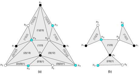
Figure 1: (a) A chromatic subdivision of a 3-process simplex; (b) Subdivision for 1-resiliency; a triangle labeled, e.g., $\{i\}\{jk\}$ corresponds to the case in which $p_{i}$ writes and reads the memory without seeing $p_{j}$ and $p_{k}$, while $p_{j}$ and $p_{k}$ saw $p_{i}$ when they read after they wrote, and they also saw each other; all possible interleavings for one write-read instruction are displayed.

Topological Invariants.

The typical approach for determining whether a task (e.g., consensus) is solvable in $t$ rounds consists of identifying topological invariants, i.e., properties of complexes that are preserved by simplicial maps. Specifically, the approach consists in:

1. Identifying a topological invariant, i.e., a property satisfied by the input complex $\mathcal{I}$, and preserved by $\Xi_{t}$;

2. Checking whether this invariant, which must be satisfied by the sub-complex $\delta(\mathcal{P}^{(t)})$ of the output complex $\mathcal{O}$, does not yield contradiction with the specification $\Delta$ of the task.

For instance, in the case of binary consensus, the input complex $\mathcal{I}_{\mbox{\scriptsize$\|$}}$ is a sphere. One basic property of spheres is being path-connected (i.e., there is a path in $\mathcal{I}_{\mbox{\scriptsize$\|$}}$ between any two vertices). As mentioned earlier, shared-memory wait-free computing corresponds to subdividing the input complex. Therefore, independently from the length $t$ of the execution, the protocol complex $\mathcal{P}^{(t)}$ is a chromatic subdivision of the sphere $\mathcal{I}_{\mbox{\scriptsize$\|$}}$, and thus it remains path-connected. On the other hand, the output complex $\mathcal{O}_{\mbox{\scriptsize$\|$}}$ of binary consensus is the disjoint union of two complexes $\mathcal{O}_{0}$ and $\mathcal{O}_{1}$, where $\mathcal{O}_{y}=\big{\{}\{(i,y):i\in I\},I\subseteq[n],I\neq\varnothing\big{\}}$ for $y\in\{0,1\}$. Since simplicial maps preserve connectivity, it follows that $\delta(\mathcal{P}^{(t)})\subseteq\mathcal{O}_{0}$ or $\delta(\mathcal{P}^{(t)})\subseteq\mathcal{O}_{1}$. As a consequence, $\delta$ cannot agree with $\Delta_{\mbox{\scriptsize$\|$}}$, as the latter maps the simplex $\{(i,0),i\in[n]\}$ to $\mathcal{O}_{0}$, and the simplex $\{(i,1),i\in[n]\}$ to $\mathcal{O}_{1}$. Therefore, consensus cannot be achieved wait-free, regardless of the number $t$ of rounds.

The fact that connectivity plays a significant role in the inability to solve consensus in the presence of asynchrony and crash failures is known since the original proof of the FLP theorem [FischerLP85] in the early 80s. However, the relation between $k$-set agreement and higher dimensional forms of connectivity (i.e., the ability to contract high dimensional spheres) was only established ten years later [HerlihyS99, SaksZ00]. We refer to [HerlihyKR2013] for numerous applications of Theorem 1.1 to various models of distributed computing, including asynchronous crash-prone shared-memory or fully-connected message passing models. In particular, for tasks such as renaming, identifying the minimal number $t$ of rounds enabling a simplicial map $\delta$ to exist is currently the only known technique for upper bounding their time complexities [AttiyaCHP19].

Network Computing.

Recently, Castañeda et al. [CastanedaFPRRT19] applied Theorem 1.1 to synchronous fault-free computing in networks, that is, to the framework in which processes are located at the vertices of an $n$-node graph $G$, and can exchange messages only along the edges of that graph. They mostly focus on input-output tasks such as consensus and set-agreement, in a simplified computing model, called KNOW-ALL, specifying that every process is initially aware of the name and the location of all the other processes in the network. As observed in [CastanedaFPRRT19], synchronous fault-free computing in the KNOW-ALL model preserves the facets of the input complex, and do not subdivide them. However, scissor cuts may occur between adjacent facets during the course of the computation, that is, the protocol complex $\mathcal{P}^{(t)}$ is obtained from the input complex $\mathcal{I}$ by partially separating facets that initially shared a simplex. Fig. 2 illustrates two types of scissor cuts applied to the sphere, corresponding to two different communication networks. The positions of the cuts depend on the structure of the graph $G$ in which the computation takes place, and determining the precise impact of the structure of $G$ on the topology of the protocol complex is a nontrivial challenge, even in the KNOW-ALL model.

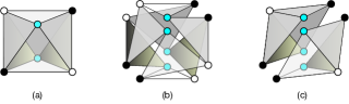
Figure 2: (a) The input complex of binary consensus for three processes; (b) The scissor cuts for the consistently directed 3-process cycle $C_{3}$ after one round; (c) The scissor cuts for the directed 3-process star $S_{3}$, where edges are directed from the center to the leaves, after one round.

Instead, we aim at analyzing classical graph problems (e.g., coloring, independent set, etc.) in the standard LOCAL model [Peleg01] of network computing, which is weaker than the KNOW-ALL model, and thus allows for more complicated topological deformations. In the LOCAL model, every node is initially aware of solely its identifier (which is unique in the network), and its input (e.g., for minimum weight vertex cover or for list-coloring), all nodes wake up synchronously, and compute in locksteps. The LOCAL model is an ideal model for studying locality in the context of network computing [Peleg01].

In addition to the fact that the topological deformations of the protocol complexes strongly depend on the structure of the network, another obstacle that makes applying the topological approach to the LOCAL model even more challenging is the presence of process identifiers. Indeed, the model typically assumes that the node IDs are taken in a range $[N]$ where $N=\operatorname{poly}(n)$. As a consequence, independently from the potential presence of other input values, the size of the complexes (i.e., their number of vertices) may become as large as ${N\choose n}n!$, since there are ${N\choose n}$ ways of choosing $n$ IDs, and $n!$ ways of assigning the $n$ chosen IDs to the $n$ nodes of $G$ (unless $G$ presents symmetries). For instance, Fig. 2 assumes the KNOW-ALL model, hence fixed IDs. Redrawing these complexes assuming that the three processes can pick arbitrary distinct IDs as in the LOCAL model, even in the small domain $\{1,2,3,4\}$, would yield a cumbersome figure with 24 nodes. Note that the presence of IDs also results in input complexes that may be topologically more complicated than pseudospheres, even for tasks such as consensus.

Importantly, the fact that the IDs are not fixed a priori, and may even be taken in a range exceeding $[n]$, is inherent to distributed network computing. This framework aims at understanding the power and limitation of computing in large networks, from LANs to the whole Internet, where the processing nodes are indeed assigned arbitrary IDs taken from a range of values which may significantly exceed the number of nodes in the network.

Objective.

To sum up, while the study of protocol complexes has found numerous applications in the context of fault-tolerant message-passing or shared-memory computing, extending this theory to network computing faces a difficulty caused by the presence of arbitrary IDs, which are often the only inputs to the processes [Peleg01]. The objective of this paper is to show how the combinatorial blowup caused by the presence of IDs in network computing can be bypassed, at least as far as local computing is concerned.

2 Our Results

We show how to bypass the aforementioned exponential blowup in the size of the complexes, that would result from a straightforward application of Theorem 1.1 for analyzing the complexity of tasks in networks. Our result holds for a variety of problems, including classical graph problems such as vertex and edge-coloring, maximal independent set (MIS), maximal matching, etc. More specifically, it holds for the large class of locally checkable labeling (LCL) tasks [NaorS95] on bounded-degree graphs. These are tasks for which it is possible to verify locally the correctness of a solution, and thus they are sometimes viewed as the analog of NP in the context of computing in networks. An LCL task is described by a finite set of labels, and a local description of how these labels can be legally assigned to the nodes of a network. Our local characterization theorem is strongly based on a seminal result by Naor and Stockmeyer [NaorS95] who showed that the values of the IDs do not actually matter much for solving LCL tasks in networks, but only their relative order matters.

We prove an analog of Theorem 1.1, but where the size of the complexes involved in the statement is independent of the size of the networks. Specifically, the size of the complexes in our characterization theorem (cf. Theorem 2.1) depends only of the maximum degree $d$ of the network, the number of labels used for the description of the task, and the number of rounds of the considered algorithm for solving that task. In particular, the identifiers are taken from a bounded-size set, even if the theorem applies to tasks defined on $n$-node networks with arbitrarily large $n$, and for identifiers taken in an arbitrarily large range $[N]$. We denote by $\mathcal{K}_{x,[y]}$ the fact that the facets of $\mathcal{K}$ have dimension $x$, and that the IDs are taken in the set $\{1,\dots,y\}$ (and let $\mathcal{K}_{x}=\mathcal{K}_{x,\varnothing}$). Our main result is the following.

Theorem 2.1 (A simplified version of Theorem LABEL:theo:main).

For every LCL task $T$ on graphs of maximum degree $d$ and every $t\geq 0$, there exists $R$ such that the following holds. The task $T$ is solvable in $t$ rounds in the LOCAL model if and only if there is a simplicial map $\delta:\mathcal{P}_{d,[R]}^{(t)}\to\mathcal{O}_{d}$ such that, for every facet $\sigma\in\mathcal{I}_{d,[R]}$, $\delta(\Xi_{t}(\sigma))\subseteq\Delta(\pi(\sigma))$.

Fig. 3 provides a rough description of the commutative diagram corresponding to the straightforward application of Theorem 1.1 to LCL tasks, and of the commutative diagram corresponding to Theorem 2.1. Note that Theorem 1.1 (the left diagram) involves global complexes with $(n-1)$-dimensional facets, whose vertices are labeled by IDs in an arbitrarily large set $[N]$. In contrast, the complexes corresponding to Theorem 2.1 (the right diagram) are local complexes, with facets of constant dimension, and vertices labeled with IDs in a finite set whose size is constant w.r.t. the number of nodes $n$ in the network. In the statement of Theorem 2.1, $\pi:\mathcal{I}_{d,[R]}\to\mathcal{I}_{d}$ is merely the mapping removing the IDs of the vertices.

Figure 3: The commutative diagrams of Theorem 1.1 (left), and Theorem 2.1 (right).

As an application of Theorem 2.1, we reformulate the celebrated lower bound $\Omega(\log^{*}n)$ rounds for 3-coloring the $n$-node ring by Linial [Linial92], in the algebraic topology framework (see Corollary LABEL:cor:reproving-linial).

3 Models and Definitions

3.1 The LOCAL model

The LOCAL model was introduced more than a quarter of a century ago (see, e.g., [Linial92, NaorS95]) for studying which tasks can be solved locally in networks, that is, which tasks can be solved when every node is bounded to collect information only from nodes in its vicinity. Specifically, the LOCAL model [Peleg01] states that the processors are located at the nodes of a simple connected graph $G=(V,E)$ modeling a network. All nodes are fault-free, they wake up simultaneously, and they execute the same algorithm. Computation proceeds in synchronous rounds, where a round consists of the following three steps performed by every node: (1) sending a message to each neighbor in $G$, (2) receiving the messages sent by the neighbors, and (3) performing local computation. There are no bounds on the size of the messages exchanged at every round between neighbors, and there are no limits on the individual computational power or memory of the nodes. These assumptions enable the design of unconditional lower bounds on the number of rounds required for performing some task (e.g., for providing the nodes with a proper coloring), while the vast majority of the algorithms solving these tasks do not abuse of these relaxed assumptions [Suomela13].

Every node in the network has an identifier (ID) which is supposed to be unique in the network. In $n$-node networks, the IDs are supposed to be in a range $1,\dots,N$ where $N\gg n$ typically holds (most often, $N=\operatorname{poly}(n)$). The absence of limits on the amount of communication and computation that can be performed at every round implies that the LOCAL model enables full-information protocols, that is, protocols in which, at every round, every node sends all the information it acquired during the previous rounds to its neighbors. Therefore, for every $t\geq 0$, and every graph $G$, a $t$-round algorithm allows every node in $G$ to acquires a local view of $G$, which is a ball in $G$ centered at that node, and of radius $t$. A view includes the inputs and the IDs of the nodes in the corresponding ball. It follows that a $t$-round algorithm in the LOCAL model can be considered as a function from the set of views of radius $t$ to the set of output values.

3.2 Locally Checkable Labelings

Let $d\geq 2$, and let $\mathcal{G}_{d}$ be the class of connected simple $d$-regular graphs. Recall that, for a positive integer $c$, $c$-coloring is the task consisting in providing each node with a color in $\{1,\dots,c\}$ in such a way that no two adjacent nodes are given the same color. MIS is the closely related task consisting in providing each node with a boolean value (0 or 1) such that no two adjacent nodes are given the value 1, and every node with value 0 is adjacent to at least one node with value 1. Proper $c$-coloring in $\mathcal{G}_{d}$ can actually be described by the collection of good stars of degree $d$, and with nodes colored by labels in $\{1,\dots,c\}$, such that the center node has a color different from the color of each leaf. Similarly, maximal independent set (MIS) in $\mathcal{G}_{d}$ can be described by the collection of stars with degree $d$, and with each node colored by a label in $\{0,1\}$, such that if the center node is labeled 1 then all the leaves are colored 0, and if the center node is labeled 0 then at least one leaf is colored 1. Other tasks such as variants of coloring, or $(2,1)$-ruling set can be described similarly, by a finite number of legal labeled stars.

More generally, given a finite set $\mathcal{L}$ of labels, we denote by $\mathbf{S}_{d}^{\mathcal{L}}$ the set of all labeled stars resulting from labeling each node of the $(d+1)$-node star by some label in $\mathcal{L}$. A locally checkable labeling (LCL) [NaorS95] is then defined by a finite set $\mathcal{L}$ of labels, and a set $\mathcal{S}\subseteq\mathbf{S}_{d}^{\mathcal{L}}$. Every star in $\mathcal{S}$ is called a good star, and those in $\mathbf{S}_{d}^{\mathcal{L}}\setminus\mathcal{S}$ are bad. The computing task defined by an LCL $(\mathcal{L},\mathcal{S})$ consists, for every node of every graph $G\in\mathcal{G}_{d}$, of computing a label in $\mathcal{L}$ such that every resulting labeled radius-1 star in $G$ is isomorphic to a star in $\mathcal{S}$. In other words, the objective of every node is to compute a label in $\mathcal{L}$ such that every resulting labeled radius-$1$ star in $G$ is good. It is undecidable, in general, whether a given LCL task has an algorithm performing in $O(1)$ rounds in the LOCAL model.

In their full generality, LCL tasks include tasks in which nodes have inputs, potentially of some restricted format. For instance, this is the case of the task consisting of reducing $c$-coloring to MIS in $C_{n}$, studied in the next section. Hence, in its full generality, an LCL task is described by a quadruple $(\mathcal{L}_{in},\mathcal{S}_{in},\mathcal{L}_{out},\mathcal{S}_{out})$ where $\mathcal{L}_{in}$ and $\mathcal{L}_{out}$ are the input and output labels, respectively. The set of stars $\mathcal{S}_{in}$ can often be simply viewed as a promise stating that every radius-1 star of the input graph $G$ belongs to $\mathcal{S}_{in}$, and the set $\mathcal{S}_{out}$ is the target set of good radius-1 stars. LCL tasks also capture settings in which the legality of the output stars depends on the inputs. A typical example of such a setting is list-coloring where the output color of each node must belong to a list of colors given to this node as input.

In fact, the framework of LCL tasks can be extended to balls of radius $r>1$, for capturing more problems, like $(\alpha,\beta)$-ruling set for large $\alpha$’s or $\beta$’s. They can also be extended to non-regular graphs with bounded maximum degree $d$. However, up to extending the set of labels, all such tasks can be reformulated in the context of radius $r=1$, and regular graphs [Brandt19]. To get the intuition of why this is true, consider the task in which every node must compute a label in $\{T,F\}$ such that every node labeled $F$ has a node labeled $T$ at distance at most $k$, for some fixed $k\geq 1$. This task can indeed be described by stars. To see how, let $\mathcal{L}=\{T,F_{1},\dots,F_{k}\}$, where we interpret the index $i$ of a label $F_{i}$ as an upper bound on the distance to a $T$-marked node. The good stars are defined as follows: a star whose center is labeled $T$ is always good, and, for $i=1,\dots,k$, a star whose center is labeled $F_{i}$ is good if there is a leaf with label in $\{T,F_{1},\dots,F_{i-1}\}$.

4 Warm Up: Coloring and MIS in the Ring

In this section, we exemplify our technique, in a way that resembles the proof of Theorem 2.1. We consider an LCL task on a ring, where the legal input stars define a proper $3$-coloring, and the output stars define a maximal independent set (MIS). That is, we study the time complexity of reducing a $3$-coloring to a MIS on a ring. It is known [Linial92] that there is a 2-round algorithm for the problem in the LOCAL model, and we show that this is optimal using topological arguments. This toy example provides the basic concepts and arguments that we use later, when considering general LCL tasks and proving Theorem 2.1.

4.1 Reduction from 3-coloring to MIS

Let us consider three consecutive nodes of the $n$-node ring $C_{n}$, denoted by $p_{-1},p_{0}$, and $p_{1}$, as displayed on Fig. 4. By the independence property, if $p_{0}$ is in the MIS, then neither $p_{-1}$ nor $p_{1}$ can be in the MIS, and, by the maximality property, if $p_{0}$ is not in the MIS, then $p_{-1}$ or $p_{1}$, or both, must be in the MIS. These constraints are captured by the complex $\mathcal{M}_{2}$ displayed on Fig. 5, including six vertices $(p_{i},x)$, with $i\in\{-1,0,1\}$, and $x\in\{0,1\}$.

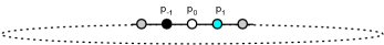
Figure 4: Three consecutive nodes in the $n$-node ring.

The complex $\mathcal{M}_{2}$ of Fig. 5 has four facets of dimension 2: they are triangles. Some triangles intersect along an edge, while some others intersect only at a node. The complex $\mathcal{M}_{2}$ is called the local complex of MIS in the ring (the index 2 refers to the fact that rings have degree 2). Note that the sets $\{(p_{-1},0),(p_{0},0),(p_{1},0)\}$ and $\{(p_{-1},1),(p_{0},1),(p_{1},1)\}$ do not form simplices of $\mathcal{M}_{2}$. We call these two sets monochromatic. In the objective of reducing 3-coloring to MIS, $\mathcal{M}_{2}$ will be the output complex, corresponding to $\mathcal{O}_{d}$ with $d=2$ in Fig. 3 and in Theorem 2.1.

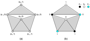
Figure 5: The local complex $\mathcal{M}_{2}$ of MIS in the ring. (a) the vertices are labeled with the index of the processes and the values; (b) the indexes of the processes are replaced by colors.

Similarly, let us focus on 3-coloring, with the same three processes $p_{-1},p_{0}$, and $p_{1}$. The neighborhood of $p_{0}$ cannot include the same color as its own color, and thus there are twelve possible colorings of the nodes in the star centered at $p_{0}$. Each of these stars corresponds to a 2-dimensional simplex, forming the facets of the local complex $\mathcal{C}_{2}$ of 3-coloring in the ring, depicted in Fig. 6. This complex contains nine vertices of the form $(p_{i},c)$, with $i\in\{-1,0,1\}$, and $c\in\{1,2,3\}$, and twelve facets. Note that the vertices $(p_{-1},3)$ and $(p_{1},3)$ appear twice in the figure, since the leftmost and rightmost edges are identified, but in opposite direction, forming a Möbius strip. $\mathcal{C}_{2}$ is a manifold (with boundary). When reducing 3-coloring to MIS, $\mathcal{C}_{2}$ will be the input complex, corresponding to $\mathcal{I}_{d}$ with $d=2$ in Fig. 3.

Figure 6: Local complex $\mathcal{C}_{2}$ of 3-coloring in the ring.

Remark.

It is crucial to note that the complexes displayed in Figs. 5 and 6 are not the ones used in the standard settings (e.g., [CastanedaFPRRT19, HerlihyKR2013]), for which Theorem 1.1 would use vertices of the form $(p,x)$ for $p\in[n]$, or even $p\in[N]$ assuming IDs in a range of $N$ values. As a consequence, these complexes have 6 vertices instead of $2n!{N\choose n}$ for MIS, and 9 vertices instead of $3n!{N\choose n}$ for coloring, where $n$ can be arbitrarily large. Even if the IDs would have been fixed, the approach of Theorem 1.1 would yield complexes with a number of vertices linear in $n$, while the complexes of Figs. 5 and 6 are of constant size.

As it is well know since the early work by Linial [Linial92], a properly 3-colored ring can be “recolored” into a MIS in just two rounds. First, the nodes colored 3 recolor themselves 1 if they have no neighbors originally colored 1. Then, the nodes colored 2 do the same, i.e., they recolor themselves 1 if they have no neighbors colored 1 (whether it be neighbors originally colored 1, or nodes that recolored themselves 1 during the first round). The nodes colored 1 output 1, and the other nodes output 0. The set of nodes colored 1 forms a MIS. Note that this algorithm is ID-oblivious, i.e., it can run in an anonymous network.

Task specification.

The specification of reducing 3-coloring to MIS can be given by the trivial carrier map $\Delta:\mathcal{C}_{2}\to 2^{\mathcal{M}_{2}}$ defined by $\Delta(F)=\{\mbox{all facets of}\;\mathcal{M}_{2}\}$ for every facet $F$ of $\mathcal{C}_{2}$. (As the LOCAL model is failure-free, it is enough to describe all maps at the level of facets.) Note that the initial coloring of a facet in $\mathcal{C}_{2}$ does not induce constraints on the facet of $\mathcal{M}_{2}$ to which it should be mapped. Fig. 7 displays some of the various commutative diagrams that will be considered in this section. In all of them, $\Delta$ is the carrier map specifying reduction from 3-coloring to MIS in the ring, and none of the simplicial maps $\delta$ exist.

Figure 7: Complexes corresponding to reduction from 3-coloring to MIS in the $n$-node ring. From left to right: 0 rounds without IDs, 1-round without IDs, 0 rounds with ID, and 1-round with IDs.

We start by considering ID-oblivious algorithms, and then move on to discussing the case of algorithms using IDs.

4.2 ID-Oblivious Algorithms

4.2.1 Impossibility in Zero Rounds

Name-preserving maps. Let us consider an alleged ID-oblivious algorithm which reduces $3$-coloring to MIS in zero rounds. Such an algorithm sees only the node’s color $c\in\{1,2,3\}$, and must map it to some $x\in\{0,1\}$. This induces a mapping $\delta$, that maps every pair $(p_{i},c)$ with $i\in\{-1,0,1\}$ and $c\in\{1,2,3\}$, to a pair $\delta(p_{i},c)=(p_{i},x)$ with $x\in\{0,1\}$. We say that such a mapping is name-preserving. By the name-preservation property, the algorithm maps the vertices in Fig. 6 to the vertices in Fig. 5(b) while preserving the names $p_{-1},p_{0},p_{1}$ of these vertices. Therefore, the algorithm induces a chromatic simplicial map $\delta:\mathcal{C}_{2}\to\mathcal{M}_{2}$. The term “chromatic” is the formal way to express that a vertex $(p,x)$ is mapped to a vertex $(p,y)$, that is, the “color” $p$, i.e., its name, is preserved.

Name-independence. Observe that the names $p_{-1},p_{0}$, and $p_{1}$ given to the nodes are “external”, i.e., they are not part of the input to the algorithm

Algorithm 2.

. That is, $(p_{i},c)$ and $(p_{j},c)$ must be mapped to $(p_{i},x)$ and $(p_{j},x)$, respectively, by the induced mapping $\delta$, for the same $x\in\{0,1\}$. We say that such a mapping $\delta$ is name-independent.

We are therefore questioning the existence of a name-preserving name-independent simplicial map $\delta:\mathcal{C}_{2}\to\mathcal{M}_{2}$. This is in correspondence to Fig. 3 and Theorem 2.1, in the degenerated case where $t=0$ and $[R]=\varnothing$, for which $\mathcal{C}_{2}=\mathcal{I}_{2}$, and $\mathcal{C}_{2,\varnothing}=\mathcal{I}_{2,\varnothing}=\mathcal{P}^{(0)}_{2,\varnothing}=\mathcal{C}_{2}$ — see the leftmost diagram in Fig. 7. It is easy to see that there cannot exist a name-preserving name-independent simplicial map $\delta$ from the manifold $\mathcal{C}_{2}$ to $\mathcal{M}_{2}$ (from Fig. 6 to Fig. 5(b)). Indeed, a simplicial map $\delta:\mathcal{C}_{2}\to\mathcal{M}_{2}$ can only map $\mathcal{C}_{2}$ entirely to the sub-complex of $\mathcal{M}_{2}$ induced by the simplex $\sigma_{00}=\{(p_{-1},0),(p_{0},1),(p_{1},0)\}$, or entirely to the sub-complex of $\mathcal{M}_{2}$ induced by all the other simplices. To see why, assume the opposite. Then, w.l.o.g., we can assume that the vertex $(p_{0},1)$ of $\mathcal{C}_{2}$ is mapped to $(p_{0},0)$ of $\mathcal{M}_{2}$, and that $(p_{0},3)$ of $\mathcal{C}_{2}$ is mapped to $(p_{0},1)$ of $\mathcal{M}_{2}$. Let us consider the two simplices

$$\{(p_{-1},2),(p_{0},1),(p_{1},2)\}\;\mbox{and}\;\{(p_{-1},2),(p_{0},3),(p_{1},2)\}$$

of $\mathcal{C}_{2}$, which form a sub-complex of $\mathcal{C}_{2}$. In order to preserve the edges of this sub-complex, $(p_{-1},2)$ and $(p_{1},2)$ must be respectively mapped to $(p_{-1},0)$ and $(p_{1},0)$. It follows that the simplex $\{(p_{-1},2),(p_{0},3),(p_{1},2)\}$ of $\mathcal{C}_{2}$ is correctly mapped to a simplex of $\mathcal{M}_{2}$ (specifically, to the simplex $\{(p_{-1},0),(p_{0},1),(p_{1},0)\}$). However, the simplex $\{(p_{-1},2),(p_{0},1),(p_{1},2)\}$ of $\mathcal{C}_{2}$ is mapped to the monochromatic set $\{(p_{-1},0),(p_{0},0),(p_{1},0)\}$ which is not a simplex of $\mathcal{M}_{2}$ (it is a hole in this complex as depicted in Fig. 5), contradiction. Thus, $\mathcal{C}_{2}$ must be entirely mapped to the sub-complex of $\mathcal{M}_{2}$ induced by the simplex $\sigma_{00}=\{(p_{-1},0),(p_{0},1),(p_{1},0)\}$, or entirely to the sub-complex of $\mathcal{M}_{2}$ induced by all the other simplices. This yields two cases:
 $-$ In the former case, $p_{0}$ outputs 1 independently from its input color, and therefore, by the name independence, $p_{-1}$ and $p_{1}$ also output 1, which is not the case in $\sigma_{00}$.
 $-$ In the latter case, $p_{0}$ outputs 0 independently from its input color, and therefore, by the name independence, $p_{-1}$ and $p_{1}$ also output 0, yielding a contradiction as no monochromatic sets are simplices of $\mathcal{M}_{2}$.
Hence, there are no name-preserving name-independent simplicial maps $\delta:\mathcal{C}_{2}\to\mathcal{M}_{2}$. The absence of a name-independent name-preserving simplicial map $\delta:\mathcal{C}_{2}\to\mathcal{M}_{2}$ is a witness of the impossibility to construct a MIS from a 3-coloring of the ring in zero rounds, when using an ID-oblivious algorithm.

4.2.2 Impossibility in One Round

For analyzing 1-round algorithms, let us consider the local protocol complex $\mathcal{P}_{2,\varnothing}^{(1)}$, including the views of the three nodes $p_{-1},p_{0}$, and $p_{1}$ after one round. The vertices of $\mathcal{P}_{2,\varnothing}^{(1)}$ are of the form $(p_{i},xyz)$ with $i\in\{-1,0,1\}$, and $x,y,z\in\{1,2,3\}$, $x\neq y$, and $y\neq z$. The vertex $(p_{i},xyz)$ is representing a process $p_{i}$ starting with color $y$, and receiving the input colors $x$ and $z$ from its left and right neighbors, respectively. The facets of $\mathcal{P}_{2,\varnothing}^{(1)}$ are of the form $\{(p_{-1},x^{\prime}xy),(p_{0},xyz),(p_{1},yzz^{\prime})\}$. Fig. 8 displays that complex, which consists of three connected components $\mathcal{K}_{1},\mathcal{K}_{2}$, and $\mathcal{K}_{3}$ where, for $y=1,2,3$, $\mathcal{K}_{y}$ includes the four vertices $(p_{0},xyz)$ for $x,z\in\{1,2,3\}\smallsetminus\{y\}$, and all triangles that include these vertices. Each set of four triangles sharing a vertex $(p_{0},xyz)$ forms a cone (see Fig. LABEL:fig:cone). These cones are displayed twisted on Fig. 8 to emphasis the “circular structure” of the three components.

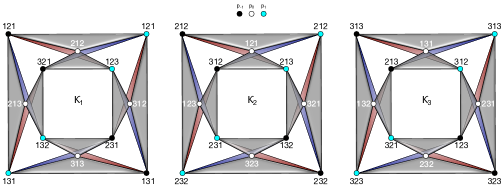
Figure 8: Local protocol complex $\mathcal{P}_{2,\varnothing}^{(1)}$ after 1 round starting from a 3-coloring of the ring.

Following the same reasoning as for 0-round algorithms, a 1-round algorithm