Structure preserving discretisations of gradient flows for axisymmetric two-phase biomembranes

Abstract

The form and evolution of multi-phase biomembranes is of fundamental importance in order to understand living systems. In order to describe these membranes, we consider a mathematical model based on a Canham–Helfrich–Evans two-phase elastic energy, which will lead to fourth order geometric evolution problems involving highly nonlinear boundary conditions. We develop a parametric finite element method in an axisymmetric setting. Using a variational approach, it is possible to derive weak formulations for the highly nonlinear boundary value problems such that energy decay laws, as well as conservation properties, hold for spatially discretised problems. We will prove these properties and show that the fully discretised schemes are well-posed. Finally, several numerical computations demonstrate that the numerical method can be used to compute complex, experimentally observed two-phase biomembranes.

Key words. biomembranes, multi-phase Canham–Helfrich–Evans energy, Willmore flow, parametric finite elements, stability, numerical simulations

AMS subject classifications. 65M60, 65M12, 35K55, 53C44

Dedicated to the memory of John W. Barrett

1 Introduction

Biomembranes and vesicles formed by lipid bilayers play a fundamental role in many living systems, and synthesised artificial vesicles are used in pharmaceutical applications as potential drug carriers. The basic structure of such membranes is a bilayer consisting of phospholipids. As the thickness of these membranes is small, the membrane is typically described as a hypersurface. It is well-known that the energy of these membranes can be modelled with the help of a curvature elasticity theory, see ????. Curvature terms in the energy account for bending stresses, but biomembranes have no or little lateral shear stresses, which hence are neglected in these elasticity models.

Often micro-domains (or rafts) are formed due to the clustering of certain molecules within the membrane. This leads to multi-phase membranes with coexisting phases. It is observed that the membrane can have a preferred curvature stemming, for example, from an asymmetry within the bilayer. This so-called spontaneous curvature can depend on the phase. Moreover, the bending rigidities appearing in the energy are typically also phase-dependent. The simplest curvature energies involve the mean curvature, but neglect the Gaussian curvature. For homogeneous biomembranes this is justified with the help of topological arguments, as long as the Gaussian bending rigidity is constant, and as long as the topology of the membrane does not change. However, for multi-phase membranes the Gaussian bending rigidity is phase-dependent, and will thus influence membrane shapes. A combination of the above phase-dependent properties can lead to a multitude of different phenomena, including budding, fingering and fusion, see ?. In this paper, we consider a geometrical evolution law of gradient flow type for two-phase biomembranes that decreases the governing energy. The energy we consider takes elastic energy as well as line energy into account. Where appropriate, the evolution will conserve volume enclosed by the membrane, as well as the areas of the appearing phases. We will derive a stable numerical method in an axisymmetric setting that is structure preserving, in the sense that a semidiscrete variant decreases energy and, when applicable, also conserves volume and areas exactly. Axisymmetric formulations numerically have the advantage that they are extremely efficient, and hence they allow for a more detailed resolution of the shapes, in particular close to budding, for example.

Based on the fundamental work of ?? we now introduce a generalised Canham–Helfrich–Evans energy for a two-phase biomembrane. The energy is defined for a two-phase surface $\mathcal{S}=(\mathcal{S}_{1},\mathcal{S}_{2})$, consisting of two sufficiently smooth surfaces ${\mathcal{S}_{i}}$, $i=1,2$, in ${\mathbb{R}}^{3}$, which have a common boundary $\gamma$ that is assumed to be a sufficiently smooth curve. In addition, it is assumed that $\mathcal{S}$ encloses a volume $\Omega(\mathcal{S})$. The energy proposed by ?? takes curvature effects, as well as line energy effects, into account, and is given by

$$E(\mathcal{S})=\sum_{i=1}^{2}\left[\tfrac{1}{2}\,\alpha_{i}\,\int_{\mathcal{S}_{i}}(k_{m,i}-{\overline{\varkappa}}_{i})^{2}\;{\rm d}{\mathcal{H}}^{2}+\alpha^{G}_{i}\,\int_{\mathcal{S}_{i}}k_{g,i}\;{\rm d}{\mathcal{H}}^{2}\right]+\varsigma\,\mathcal{H}^{1}(\gamma)\,.$$ (1.1)

Here the constants $\alpha_{i}\in{\mathbb{R}}_{>0}$ and $\alpha^{G}_{i}\in{\mathbb{R}}$ are the mean and the Gaussian bending rigidities of the two phases, and the constants ${\overline{\varkappa}}_{i}\in{\mathbb{R}}$ are the spontaneous curvatures. Note that all these quantities might attain different values in the two phases. Moreover, $k_{m,i}$ and $k_{g,i}$ denote the mean and the Gaussian curvature of $\mathcal{S}_{i}$, $i=1,2$, and $\varsigma$ is the energy density of the interface, often called line tension. Finally, $\mathcal{H}^{2}$ and $\mathcal{H}^{1}$ are the surface and length measures in ${\mathbb{R}}^{3}$.

For the attachment conditions on $\gamma$ two cases have been considered in the literature, see ??:

$$C^{0} \quad\gamma=\partial\mathcal{S}_{1}=\partial\mathcal{S}_{2}\,,$$–case : (1.2a)

$$C^{1} \quad\gamma=\partial\mathcal{S}_{1}=\partial\mathcal{S}_{2}\quad\text{ and }\quad\vec{\rm n}_{\mathcal{S}_{1}}=\vec{\rm n}_{\mathcal{S}_{2}}\quad\text{on }\gamma\,,$$–case : (1.2b)

where $\vec{\rm n}_{\mathcal{S}_{i}}$ denotes the outer unit normal of $\mathcal{S}_{i}$. Of course, in the case (1.2b) it also holds that $\vec{\mu}_{\partial\mathcal{S}_{1}}=-\vec{\mu}_{\partial\mathcal{S}_{2}}$, where $\vec{\mu}_{\partial\mathcal{S}_{i}}$ denotes the outer unit conormal to $\mathcal{S}_{i}$ on $\gamma$.

It is discussed in ? that the contributions

$$\sum_{i=1}^{2}\left[\tfrac{1}{2}\,\alpha_{i}\,\int_{\mathcal{S}_{i}}k_{m,i}^{2}\;{\rm d}{\mathcal{H}}^{2}+\alpha^{G}_{i}\,\int_{\mathcal{S}_{i}}k_{g,i}\;{\rm d}{\mathcal{H}}^{2}\right]$$

to the energy (1.1) are nonnegative if

$$\alpha^{G}_{i}\in[-2\,\alpha_{i},0]\,,\ i=1,2\,.$$

In the $C^{1}$–case, recall (1.2b), however, one can use the Gauss–Bonnet theorem, see (1.4) below, to show that the energy (1.1), when restricted to a fixed topology, can be bounded from below if $\alpha^{G}_{i}\geq\max\{\alpha^{G}_{1},\alpha^{G}_{2}\}-2\,\alpha_{i}$ for $i=1,2$, which will hold whenever

$$\min\{\alpha_{1},\alpha_{2}\}\geq\tfrac{1}{2}\,|\alpha^{G}_{1}-\alpha^{G}_{2}|\,,$$ (1.3)

see ?? for details.

It is crucial for a numerical treatment that the Gaussian curvature term can be computed efficiently in the discrete setting. In this context, a reformulation of the energy using the Gauss–Bonnet theorem is important. In fact, the Gauss–Bonnet theorem yields

$$\int_{\mathcal{S}_{i}}k_{g,i}\;{\rm d}{\mathcal{H}}^{2}=2\,\pi\,m(\mathcal{S}_{i})+\int_{\partial\mathcal{S}_{i}}k_{\partial\mathcal{S}_{i},\mu}\;{\rm d}{\mathcal{H}}^{1}\,,$$ (1.4)

where $m(\mathcal{S}_{i})\in\mathbb{Z}$ denotes the Euler characteristic of $\mathcal{S}_{i}$ and $k_{\partial\mathcal{S}_{i},\mu}$ is the geodesic curvature of $\partial\mathcal{S}_{i}$. Using this equality for the integrated Gaussian curvature, we can rewrite the energy (1.1) as

$$E(\mathcal{S})=\sum_{i=1}^{2}\left[\tfrac{1}{2}\,\alpha_{i}\,\int_{\mathcal{S}_{i}}(k_{m,i}-{\overline{\varkappa}}_{i})^{2}\;{\rm d}{\mathcal{H}}^{2}+\alpha^{G}_{i}\left[\int_{\gamma}k_{\partial\mathcal{S}_{i},\mu}\;{\rm d}{\mathcal{H}}^{1}+2\,\pi\,m(\mathcal{S}_{i})\right]\right]+\varsigma\,\mathcal{H}^{1}(\gamma)\,.$$ (1.5)

We now need to compute the geodesic curvatures $k_{\partial\mathcal{S}_{i},\mu}$. In order to do so, we first define the conormal, $\vec{\mu}_{\partial\mathcal{S}_{i}}$, to $\mathcal{S}_{i}$ on $\gamma$ to be

$$\vec{\mu}_{\partial\mathcal{S}_{i}}=\pm\,\vec{\rm n}_{\mathcal{S}_{i}}\times\vec{\rm}id_{s}\quad\text{on }\gamma\,,\ i=1,2\,,$$ (1.6)

where $\vec{\rm}id$ denotes the identity in ${\mathbb{R}}^{3}$ and $s$ denotes arclength on the curve $\gamma\subset{\mathbb{R}}^{3}$, and the sign in (1.6) is chosen so that $\vec{\mu}_{\partial\mathcal{S}_{i}}$ points out of $\mathcal{S}_{i}$, $i=1,2$. It holds that

$$\vec{\rm}id_{ss}=\vec{k}_{\gamma}=k_{\partial\mathcal{S}_{i},\rm n}\,\vec{\rm n}_{\mathcal{S}_{i}}+k_{\partial\mathcal{S}_{i},\mu}\,\vec{\mu}_{\partial\mathcal{S}_{i}}\quad\text{on }\gamma\,,\ i=1,2\,,$$ (1.7)

where $\vec{k}_{\gamma}$ is the curvature vector on $\gamma$, and where $k_{\partial\mathcal{S}_{i},\rm n}$ is the normal curvature and $k_{\partial\mathcal{S}_{i},\mu}$ is the geodesic curvature of $\partial\mathcal{S}_{i}$, $i=1,2$.

In applications for biomembranes, cf. ??, the surface areas of $\mathcal{S}_{1}$ and $\mathcal{S}_{2}$ need to stay constant during the evolution, as well as the volume of the set $\Omega(\mathcal{S})$ enclosed by $\mathcal{S}$. In this case one can consider the energy

$$E_{\lambda}(\mathcal{S})=E(\mathcal{S})+\lambda_{V}\,\mathcal{L}^{3}(\Omega(\mathcal{S}))+\sum_{i=1}^{2}\lambda_{A,i}\,\mathcal{H}^{2}(\mathcal{S}_{i})\,,$$ (1.8)

where $\mathcal{L}^{3}$ denotes the Lebesgue measure in $\mathbb{R}^{3}$. Here $\lambda_{A,i}$ are Lagrange multipliers for the area constraints, which can be interpreted as a surface tension, and $\lambda_{V}$ is a Lagrange multiplier for the volume constraint, which might be interpreted as a pressure difference.

We now introduce the governing evolution equations that we consider in this paper. We will consider the $L^{2}$–gradient flow of the energy $E_{\lambda}$, leading to a time-dependent family of surfaces $\mathcal{S}(t)$ and time-dependent Lagrange multipliers $\lambda_{V}(t)$ and $\lambda_{A,i}(t)$, $i=1,2$. This will lead to an equation for the normal velocity of the surfaces $\mathcal{S}_{i}$, $i=1,2$, as well as to equations on the curve $\gamma$. The reformulation (1.5) of the energy shows that a variation of the energy, which only affects points away from $\gamma$, will not change the Gaussian curvature part of the energy. This is reflected by the fact that, in the gradient flow formulation, the normal velocities $\mathcal{V}_{\mathcal{S}_{i}}$ on the surfaces $\mathcal{S}_{i}$, $i=1,2$, do not contain terms stemming from the Gaussian curvature contribution to the energy. In fact, we have from ?, (2.16) that

$$\mathcal{V}_{\mathcal{S}_{i}} =-\alpha_{i}\,\Delta_{\mathcal{S}_{i}}\,k_{m,i}+\tfrac{1}{2}\,\alpha_{i}\,(k_{m,i}-{\overline{\varkappa}}_{i})^{2}\,k_{m,i}-\alpha_{i}\,(k_{m,i}-{\overline{\varkappa}}_{i})\,|\nabla_{\!\mathcal{S}_{i}}\,\vec{\rm n}_{\mathcal{S}_{i}}|^{2}+\lambda_{A,i}\,k_{m,i}-\lambda_{V}$$

$$=-\alpha_{i}\,\Delta_{\mathcal{S}_{i}}\,k_{m,i}+2\,\alpha_{i}\,(k_{m,i}-{\overline{\varkappa}}_{i})\,k_{g,i}-\left[\tfrac{1}{2}\,\alpha_{i}\,(k_{m,i}^{2}-{\overline{\varkappa}}_{i}^{2})-\lambda_{A,i}\right]k_{m,i}-\lambda_{V}$$

$$\hskip 256.0748pt\quad\text{on }\mathcal{S}_{i}(t)\,,\ i=1,2\,,$$ (1.9)

where $\Delta_{\mathcal{S}_{i}}$ and $\nabla_{\!\mathcal{S}_{i}}$ denote the surface Laplacian and surface gradient on $\mathcal{S}_{i}$, respectively, and where we have observed that $|\nabla_{\!\mathcal{S}_{i}}\,\vec{\rm n}_{\mathcal{S}_{i}}|^{2}=k_{m,i}^{2}-2\,k_{g,i}$, see e.g. ?, Lemma 12(iv).

However, the Gaussian curvature energy contributions have an effect on the boundary. In the $C^{0}$–junction case, for $t\in[0,T]$, the boundary conditions on $\gamma(t)$ are given by

$$\alpha_{i}\,(k_{m,i}-{\overline{\varkappa}}_{i})+\alpha^{G}_{i}\,\vec{k}_{\gamma}\,.\,\vec{\rm n}_{\mathcal{S}_{i}}=0\,,\ i=1,2\,,$$ (1.10a)

$$\sum_{i=1}^{2}\left[(\alpha_{i}\,(\nabla_{\!\mathcal{S}_{i}}\,k_{m,i})\,.\,\vec{\mu}_{\partial\mathcal{S}_{i}}-\alpha^{G}_{i}\,(\mathfrak{t}_{i})_{s})\,\vec{\rm n}_{\mathcal{S}_{i}}-(\tfrac{1}{2}\,\alpha_{i}\,(k_{m,i}-{\overline{\varkappa}}_{i})^{2}+\alpha^{G}_{i}\,k_{g,i}+\lambda_{A,i})\,\vec{\mu}_{\partial\mathcal{S}_{i}}\right]$$

$$\qquad+\varsigma\,\vec{k}_{\gamma}=\vec{0}\,,$$ (1.10b)

see ?, (2.19), where $\mathfrak{t}_{i}=-(\vec{\rm n}_{\mathcal{S}_{i}})_{s}\,.\,\vec{\mu}_{\partial\mathcal{S}_{i}}$ is the geodesic torsion of $\gamma(t)$ on $\mathcal{S}_{i}(t)$. In case of a $C^{1}$–junction, we have that $\vec{\rm n}_{\mathcal{S}}=\vec{\rm n}_{\mathcal{S}_{1}}=\vec{\rm n}_{\mathcal{S}_{2}}$ and $\vec{\mu}_{\partial\mathcal{S}}=\vec{\mu}_{\partial\mathcal{S}_{2}}=-\vec{\mu}_{\partial\mathcal{S}_{1}}$ at the junction, and the governing equations on the curve $\gamma(t)$ for $t\in[0,T]$ are

$$[\alpha_{i}\,(k_{m,i}-{\overline{\varkappa}}_{i})]_{1}^{2}+[\alpha^{G}_{i}]_{1}^{2}\,\vec{k}_{\gamma}\,.\,\vec{\rm n}_{\mathcal{S}}=0\,,$$ (1.11a)

$$[\alpha_{i}\,(\nabla_{\!\mathcal{S}_{i}}\,k_{m,i})]_{1}^{2}\,.\,\vec{\mu}_{\partial\mathcal{S}}+\varsigma\,\vec{k}_{\gamma}\,.\,\vec{\rm n}_{\mathcal{S}}-[\alpha^{G}_{i}]_{1}^{2}\,\mathfrak{t}_{s}=0\,,$$ (1.11b)

$$[-\tfrac{1}{2}\,\alpha_{i}\,(k_{m,i}-{\overline{\varkappa}}_{i})^{2}+\alpha_{i}\,(k_{m,i}-{\overline{\varkappa}}_{i})\,(k_{m,i}-\vec{k}_{\gamma}\,.\,\vec{\rm n}_{\mathcal{S}})-\lambda_{A,i}]_{1}^{2}+[\alpha^{G}_{i}]_{1}^{2}\,\mathfrak{t}^{2}+\varsigma\,\vec{k}_{\gamma}\,.\,\vec{\mu}_{\mathcal{S}}=0\,,$$ (1.11c)

see ?, (2.20), where $[a_{i}]_{1}^{2}=a_{2}-a_{1}$ denotes the jump of the quantity $a$ across $\gamma(t)$, and where $\mathfrak{t}=\mathfrak{t}_{2}=-\mathfrak{t}_{1}$.

For more basic information on the biophysics of vesicles and biomembranes we refer to ?. Two-component membranes are discussed in ?????????.

Many mathematical results are known on the problem of minimising the Willmore and Helfrich functional, see ???, and for the corresponding gradient flows, see ??. However, problems involving the multi-phase Canham–Helfrich–Evans have not been treated mathematically in much detail yet. We refer to ???? for first results. Available related results for the corresponding gradient flow are restricted to boundary value problems for Willmore flow with line tension, cf. ?, and to the evolution of elastic flows with junctions, see ??.

Numerical approaches for the evolution of two-phase membranes often rely on phase field methods, see ??????. ? numerically studied solutions for the shape equations for two-phase vesicles numerically and ? solved the gradient flow dynamics of two-phase biomembranes formulated in a sharp interface setting numerically. A numerical method for the evolution of elastic flows with junctions has been proposed in ?. In this paper, we will present a parametric finite element method for the $L^{2}$–gradient flow of (1.8) in an axisymmetric setting. Throughout the paper, we will make extensive use of our recent work ?, in which the analogous gradient flow for a more general energy for a single surface has been treated.

The outline of the paper is as follows. In Section 2 we derive the axisymmetric version of the governing equations. For the finite element method it is important to derive a weak formulation for the highly nonlinear problem. This is done in Section 3 using an approach based on a Lagrangian method. In Section 4 a semidiscretisation is developed which preserves important energy decay and conservation properties. In Section 5 we analyze a fully discrete version of the method developed in the previous section and show that the resulting equations are well-posed. Numerical results are given in Section 6 and a comparison with the seminal experimental paper by ? is given. Finally, in an Appendix, we show that the weak formulation introduced in Section 3 is consistent with the strong formulation.

Figure 1: Sketch of $\Gamma_{i}$ and $\mathcal{S}_{i}$, $i=1,2$, as well as the unit vectors $\vec{e}_{1}$, $\vec{e}_{2}$ and $\vec{e}_{3}$.

2 The axisymmetric setting

For the axisymmetric setting, we assume that $\vec{x}_{i}(t):\overline{I}_{i}\to{\mathbb{R}}_{\geq 0}\times{\mathbb{R}}$ are parameterisations of $\Gamma_{i}(t)$, $i=1,2$, with $I_{1}=(0,\frac{1}{2})$ and $I_{2}=(\frac{1}{2},1)$, and such that $\vec{x}_{1}(\tfrac{1}{2},t)=\vec{x}_{2}(\tfrac{1}{2},t)$ and $\vec{x}_{i}(\rho,t)\,.\,\vec{e}_{1}=0$ if and only if $\rho\in\partial I_{i}\setminus\{\frac{1}{2}\}$, $i=1,2$, for all $t\in[0,T]$. Throughout $\Gamma_{i}(t)$ represents the generating curve of a surface $\mathcal{S}_{i}(t)$ that is axisymmetric with respect to the $x_{2}$–axis, see Figure 1. In particular, on defining

$$\vec{\Pi}_{3}^{3}(r,z,\theta)=(r\,\cos\theta,z,r\,\sin\theta)^{T}\quad\text{for}\quad r\in{\mathbb{R}}_{\geq 0}\,,\ z\in{\mathbb{R}}\,,\ \theta\in[0,2\,\pi]$$

and $\Pi_{2}^{3}(r,z)=\{\vec{\Pi}_{3}^{3}(r,z,\theta):\theta\in[0,2\,\pi)\}$, we have that

$$\mathcal{S}_{i}(t)=\bigcup_{(r,z)^{T}\in\Gamma_{i}(t)}\Pi_{2}^{3}(r,z)=\bigcup_{\rho\in\overline{I}_{i}}\Pi_{2}^{3}(\vec{x}_{i}(\rho,t))\quad\text{and}\quad\gamma(t)=\Pi_{2}^{3}(\vec{x}_{1}(\tfrac{1}{2},t))=\Pi_{2}^{3}(\vec{x}_{2}(\tfrac{1}{2},t))\,.$$ (2.1)

On assuming, for $t\in[0,T]$ and $i=1,2$, that

$$|[\vec{x}_{i}]_{\rho}|\geq c_{0}>0\qquad\forall\ \rho\in\overline{I}_{i}\,,$$

we introduce the arclength $s$ of the curves, i.e. $\partial_{s}=|[\vec{x}_{i}]_{\rho}|^{-1}\,\partial_{\rho}$ in $I_{i}$, and set

$$\vec{\tau}_{i}(\rho,t)=[\vec{x}_{i}]_{s}(\rho,t)=\frac{[\vec{x}_{i}]_{\rho}(\rho,t)}{|[\vec{x}_{i}]_{\rho}(\rho,t)|}\quad\text{and}\quad\vec{\nu}_{i}(\rho,t)=-[\vec{\tau}_{i}(\rho,t)]^{\perp}\quad\text{in }\overline{I}_{i}\,,$$ (2.2)

where $(\cdot)^{\perp}$ denotes a clockwise rotation by $\frac{\pi}{2}$. Then the normal velocity $\mathcal{V}_{\mathcal{S}_{i}}$ of $\mathcal{S}_{i}(t)$ in the direction $\vec{\rm n}_{\mathcal{S}_{i}}$ is given by

$$\mathcal{V}_{\mathcal{S}_{i}}=[\vec{x}_{i}]_{t}(\rho,t)\,.\,\vec{\nu}_{i}(\rho,t)\quad\text{on }\Pi_{2}^{3}(\vec{x}_{i}(\rho,t))\subset\mathcal{S}_{i}(t)\quad\forall\ \rho\in\overline{I}_{i}\,,\ t\in[0,T]\,,\ i=1,2\,.$$

For the curvature $\varkappa_{i}$ of $\Gamma_{i}(t)$ it holds that

$$\varkappa_{i}\,\vec{\nu}_{i}=\vec{\varkappa}_{i}=[\vec{\tau}_{i}]_{s}=\frac{1}{|[\vec{x}_{i}]_{\rho}|}\left[\frac{[\vec{x}_{i}]_{\rho}}{|[\vec{x}_{i}]_{\rho}|}\right]_{\rho}\quad\text{in }\ \overline{I}_{i}\,,\ i=1,2\,.$$ (2.3)

We recall that the mean curvature and Gaussian curvature of $\mathcal{S}_{i}(t)$ are then given by

$$\varkappa_{\mathcal{S}_{i}}=\varkappa_{i}-\frac{\vec{\nu}_{i}\,.\,\vec{e}_{1}}{\vec{x}_{i}\,.\,\vec{e}_{1}}\quad\text{and}\quad{\mathcal{K}}_{\mathcal{S}_{i}}=-\varkappa_{i}\,\frac{\vec{\nu}_{i}\,.\,\vec{e}_{1}}{\vec{x}_{i}\,.\,\vec{e}_{1}}=\varkappa_{i}\,(\varkappa_{\mathcal{S}_{i}}-\varkappa_{i})\quad\text{in }\ \overline{I}_{i}\,,\ i=1,2\,,$$ (2.4)

respectively; see (B.7) in Appendix B. More precisely, if $k_{m,i}$ and $k_{g,i}$ denote the mean and Gaussian curvatures of $\mathcal{S}_{i}(t)$, then

$$k_{m,i}=\varkappa_{\mathcal{S}_{i}}(\rho,t)\ \text{ and }\ k_{g,i}={\mathcal{K}}_{\mathcal{S}_{i}}(\rho,t)\quad\text{on }\Pi_{2}^{3}(\vec{x}_{i}(\rho,t))\subset\mathcal{S}_{i}(t)\quad\forall\ \rho\in\overline{I}_{i}\,,\ t\in[0,T]\,.$$

Clearly, for a smooth surface with bounded curvatures it follows from (2.4) that

$$\vec{\nu}_{i}(\rho,t)\,.\,\vec{e}_{1}=0\qquad\forall\ \rho\in\partial I_{i}\setminus\{\tfrac{1}{2}\}\,,\quad\forall\ t\in[0,T]\,,\ i=1,2\,,$$ (2.5)

which is equivalent to

$$[\vec{x}_{i}]_{\rho}(\rho,t)\,.\,\vec{e}_{2}=0\qquad\forall\ \rho\in\partial I_{i}\setminus\{\tfrac{1}{2}\}\,,\quad\forall\ t\in[0,T]\,,\ i=1,2\,.$$ (2.6)

We note that for the singular fraction in (2.4) it follows from (2.6) and (2.5), on recalling (2.3), that

$$\lim_{\rho\to\rho_{0}}\frac{\vec{\nu}_{i}(\rho,t)\,.\,\vec{e}_{1}}{\vec{x}_{i}(\rho,t)\,.\,\vec{e}_{1}} =\lim_{\rho\to\rho_{0}}\frac{[\vec{\nu}_{i}]_{\rho}(\rho,t)\,.\,\vec{e}_{1}}{[\vec{x}_{i}]_{\rho}(\rho,t)\,.\,\vec{e}_{1}}=[\vec{\nu}_{i}]_{s}(\rho_{0},t)\,.\,\vec{\tau}_{i}(\rho_{0},t)=-\varkappa_{i}(\rho_{0},t)$$

$$\hskip 85.35826pt\quad\forall\ \rho_{0}\in\partial I_{i}\setminus\{\tfrac{1}{2}\}\,,\ \forall\ t\in[0,T]\,,\ i=1,2\,.$$ (2.7)

Moreover, on recalling (1.7), it is easily seen that

$$k_{\partial\mathcal{S}_{i},\rm n}=-\frac{\vec{\nu}_{i}(\tfrac{1}{2},t)\,.\,\vec{e}_{1}}{\vec{x}_{i}(\tfrac{1}{2},t)\,.\,\vec{e}_{1}}\ \text{ and }\ k_{\partial\mathcal{S}_{i},\mu}=-\frac{\vec{\mu}_{i}(\tfrac{1}{2},t)\,.\,\vec{e}_{1}}{\vec{x}_{i}(\tfrac{1}{2},t)\,.\,\vec{e}_{1}}\quad\text{on }\gamma(t)\quad\forall\ t\in[0,T]\,,\ i=1,2\,,$$ (2.8)

where $\vec{\nu}_{i}(\cdot,t)$ is the unit normal on $\Gamma_{i}(t)$ as defined in (2.2), and where

$$\vec{\mu}_{1}(\tfrac{1}{2},t)=\vec{\tau}_{1}(\tfrac{1}{2},t)\,,\ \vec{\mu}_{2}(\tfrac{1}{2},t)=-\vec{\tau}_{2}(\tfrac{1}{2},t)\quad\forall\ t\in[0,T]\,,$$ (2.9)

denotes the corresponding conormals of $\Gamma_{i}(t)$ at the endpoint $\vec{x}_{1}(\tfrac{1}{2},t)=\vec{x}_{2}(\tfrac{1}{2},t)$. Here we have recalled that the conormal $\vec{\mu}_{\partial\mathcal{S}_{i}}$ points out of $\mathcal{S}_{i}(t)$.

We consider the following axisymmetric energy that is equivalent to (1.5) for flows of axisymmetric surfaces without topological changes

$$\widetilde{E}(\vec{x}(t))=E(\mathcal{S}(t))-2\,\pi\,\sum_{i=1}^{2}\alpha^{G}_{i}\,m(\mathcal{S}_{i}(t))$$

$$\quad=\sum_{i=1}^{2}\left[\pi\,\alpha_{i}\,\int_{I_{i}}\vec{x}_{i}\,.\,\vec{e}_{1}\left[\varkappa_{\mathcal{S}_{i}}-{\overline{\varkappa}}_{i}\right]^{2}|[\vec{x}_{i}]_{\rho}|\;{\rm d}\rho\right]-2\,\pi\,\sum_{i=1}^{2}\alpha^{G}_{i}\,\vec{\mu}_{i}(\tfrac{1}{2})\,.\,\vec{e}_{1}+\pi\,\varsigma\,\sum_{i=1}^{2}\vec{x}_{i}(\tfrac{1}{2})\,.\,\vec{e}_{1}\,.$$ (2.10)

In a similar fashion, we define an axisymmetric analogue of (1.8) as

$$\widetilde{E}_{\lambda}(\vec{x}(t))=\widetilde{E}(\vec{x}(t))+\sum_{i=1}^{2}\lambda_{A,i}\,A(\vec{x}(t))+\lambda_{V}\,V(\vec{x}(t))\,,$$ (2.11)

where we have defined, observe (B.4) in Appendix B,

$$A_{i}(\vec{x}(t))=2\,\pi\,\int_{I_{i}}\vec{x}_{i}\,.\,\vec{e}_{1}\,|[\vec{x}_{i}]_{\rho}|\;{\rm d}\rho=\mathcal{H}^{2}(\mathcal{S}_{i}(t))$$ (2.12)

and, see e.g. ?, (3.10),

$$V(\vec{x}(t))=\pi\sum_{i=1}^{2}\int_{I_{i}}(\vec{x}_{i}\,.\,\vec{e}_{1})^{2}\,\vec{\nu}_{i}\,.\,\vec{e}_{1}\,|[\vec{x}_{i}]_{\rho}|\;{\rm d}\rho=\mathcal{L}^{3}(\Omega(t))\,.$$ (2.13)

For later use we observe that

$$\frac{\rm d}{{\rm d}t}\,A_{i}(\vec{x}(t))=2\,\pi\int_{I_{i}}\left[[\vec{x}_{i}]_{t}\,.\,\vec{e}_{1}\,|[\vec{x}_{i}]_{\rho}|+(\vec{x}_{i}\,.\,\vec{e}_{1})\,([\vec{x}_{i}]_{t})_{\rho}\,.\,\vec{\tau}_{i}\right]\;{\rm d}\rho\,,\ i=1,2\,,$$ (2.14)

and

$$\frac{\rm d}{{\rm d}t}\,V(\vec{x}(t))=2\,\pi\,\sum_{i=1}^{2}\int_{I_{i}}(\vec{x}_{i}\,.\,\vec{e}_{1})\,[\vec{x}_{i}]_{t}\,.\,\vec{\nu}_{i}\,|[\vec{x}_{i}]_{\rho}|\;{\rm d}\rho\,.$$ (2.15)

The axisymmetric formulation of the gradient flow (1.9) is now given by

$$(\vec{x}_{i}\,.\,\vec{e}_{1})\,[\vec{x}_{i}]_{t}\,.\,\vec{\nu}_{i} =-\alpha_{i}\,[\vec{x}_{i}\,.\,\vec{e}_{1}\,(\varkappa_{\mathcal{S}_{i}})_{s}]_{s}+2\,\alpha_{i}\,\vec{x}_{i}\,.\,\vec{e}_{1}\,(\varkappa_{\mathcal{S}_{i}}-{\overline{\varkappa}}_{i})\,{\mathcal{K}}_{\mathcal{S}_{i}}$$

$$\quad-\vec{x}_{i}\,.\,\vec{e}_{1}\left[\tfrac{1}{2}\,\alpha_{i}\,(\varkappa_{\mathcal{S}_{i}}^{2}-{\overline{\varkappa}}^{2}_{i})-\lambda_{A,i}\right]\varkappa_{\mathcal{S}_{i}}-\lambda_{V}\,\vec{x}_{i}\,.\,\vec{e}_{1}\quad\text{in }\ \overline{I}_{i}\,,\ i=1,2\,,$$ (2.16)

where for the first term on the right hand side of (2) we have observed (B.5) in Appendix B. At an interface between the two phases, we require axisymmetric versions of the boundary conditions (1.10) and (1.11). First of all, we notice that the geodesic torsion $\mathfrak{t}_{i}$ of $\gamma(t)$ with respect to $\mathcal{S}_{i}$, $i=1,2$, is zero in the axisymmetric setting and hence the terms involving the geodesic torsion vanish, see also ?, (2.25). In the $C^{0}$–case, relating to (1.10), we have for the axisymmetric situation the following conditions at the point $\rho=\frac{1}{2}$ and for $t\in[0,T]$:

$$\alpha_{i}\,(\varkappa_{\mathcal{S}_{i}}-{\overline{\varkappa}}_{i})-\alpha^{G}_{i}\,\frac{\vec{\nu}_{i}\,.\,\vec{e}_{1}}{\vec{x}\,.\,\vec{e}_{1}}=0\,,\quad i=1,2\,,$$ (2.17a)

$$\sum_{i=1}^{2}\left[(-1)^{i-1}\,\alpha_{i}\,(\varkappa_{\mathcal{S}_{i}})_{s}\,\vec{\nu}_{i}-\left(\tfrac{1}{2}\,\alpha_{i}\,(\varkappa_{\mathcal{S}_{i}}-{\overline{\varkappa}}_{i})^{2}+\alpha_{i}^{G}\,{\mathcal{K}}_{\mathcal{S}_{i}}+\lambda_{A,i}\right)\vec{\mu}_{i}\right]-\frac{\varsigma}{\vec{x}\,.\,\vec{e}_{1}}\,\vec{e}_{1}=\vec{0}\,,$$ (2.17b)

where we used the notation $\vec{x}=\vec{x}_{1}=\vec{x}_{2}$ at $\rho=\frac{1}{2}$. For the $C^{1}$–case, and so corresponding to (1.11), we obtain at $\rho=\frac{1}{2}$ and for $t\in[0,T]$:

$$[\alpha_{i}\,(\varkappa_{\mathcal{S}_{i}}-{\overline{\varkappa}}_{i})]_{1}^{2}-[\alpha^{G}_{i}]_{1}^{2}\,\frac{\vec{\nu}\,.\,\vec{e}_{1}}{\vec{x}\,.\,\vec{e}_{1}}=0\,,$$ (2.18a)

$$-[\alpha_{i}\,(\varkappa_{\mathcal{S}_{i}})_{s}]_{1}^{2}-\varsigma\,\frac{\vec{\nu}\,.\,\vec{e}_{1}}{\vec{x}\,.\,\vec{e}_{1}}=0\,,$$ (2.18b)

$$[-\tfrac{1}{2}\,\alpha_{i}\,(\varkappa_{\mathcal{S}_{i}}-{\overline{\varkappa}}_{i})^{2}+\alpha_{i}\,(\varkappa_{\mathcal{S}_{i}}-{\overline{\varkappa}}_{i})\,\varkappa_{i}-\lambda_{A,i}]_{1}^{2}-\varsigma\,\frac{\vec{\mu}\,.\,\vec{e}_{1}}{\vec{x}\,.\,\vec{e}_{1}}=0\,,$$ (2.18c)

where we have defined $\vec{\nu}=\vec{\nu}_{1}=\vec{\nu}_{2}$ and $\vec{\mu}=\vec{\mu}_{2}=-\vec{\mu}_{1}$ at $\rho=\frac{1}{2}$, and where we have used (1.7), (2.4) and (2.8).

Finally, we impose the following boundary conditions at the axis of rotation, for $t\in[0,T]$:

$$\vec{x}_{i}\,.\,\vec{e}_{1} =0\ \text{on }\partial I_{i}\setminus\{\tfrac{1}{2}\}\,,$$ (2.19a)

$$[\vec{x}_{i}]_{\rho}\,.\,\vec{e}_{2} =0\ \text{on }\partial I_{i}\setminus\{\tfrac{1}{2}\}\,,$$ (2.19b)

$$[\varkappa_{\mathcal{S}_{i}}]_{\rho} =0\ \text{on }\partial I_{i}\setminus\{\tfrac{1}{2}\}\,.$$ (2.19c)

Here (2.19c) ensures that the radially symmetric functions on $\mathcal{S}_{i}(t)$ induced by $\varkappa_{{\mathcal{S}}_{i}}$, $i=1,2$, are differentiable, while (2.19b) is the same as (2.6).

Clearly, for surface area and volume conserving flows, the Lagrange multipliers $(\lambda_{A,1}(t),\lambda_{A,2}(t),\lambda_{V}(t))^{T}\in{\mathbb{R}}^{3}$ in (2) need to be chosen such that

$$\frac{\rm d}{{\rm d}t}\,\int_{I_{i}}\vec{x}_{i}\,.\,\vec{e}_{1}\,|[\vec{x}_{i}]_{\rho}|\;{\rm d}\rho=0\,,\ i=1,2\,,\qquad\frac{\rm d}{{\rm d}t}\,\sum_{i=1}^{2}\left((\vec{x}_{i}\,.\,\vec{e}_{1})^{2},\vec{\nu}_{i}\,.\,\vec{e}_{1}\,|[\vec{x}_{i}]_{\rho}|\right)=0\,,$$ (2.20)

where we recall (2.14) and (2.15).

3 Weak formulation

Using the formal calculus of PDE constrained optimisation, in this section we derive a weak formulation for the gradient flow (2). The necessary techniques are described in ?, §9.3, and details for the case of a one-phase axisymmetric surface can be found in ?, §3.1. The fact that the obtained weak formulation is indeed consistent with (2) and the boundary conditions (2.17), (2.18) and (2.19) will be shown in Appendix A.

We begin by defining the following function spaces. Let

$$\mathbb{X}_{i} =\{\vec{\eta}_{i}\in[H^{1}(I_{i})]^{2}:\vec{\eta}_{i}(\rho)\,.\,\vec{e}_{1}=0\quad\forall\ \rho\in\partial I_{i}\setminus\{\tfrac{1}{2}\}\}\,,\ i=1,2\,,$$

$$\mathbb{X} =\{(\vec{\eta}_{1},\vec{\eta}_{2})\in\mathop{\times}_{i=1}^{2}:\mathbb{X}_{i}:\vec{\eta}_{1}(\tfrac{1}{2})=\vec{\eta}_{2}(\tfrac{1}{2})\}\,,$$

as well as $\mathbb{Y}=\mathbb{Y}_{1}\times\mathbb{Y}_{2}$, with $\mathbb{Y}_{i}=\mathbb{X}_{i}$, $i=1,2$, and

$$\mathbb{Y}_{C^{0}}=\{(\vec{\eta}_{1},\vec{\eta}_{2})\in\mathbb{Y}:\vec{\eta}_{1}(\tfrac{1}{2})=\vec{\eta}_{2}(\tfrac{1}{2})=\vec{0}\}\,,\quad\mathbb{Y}_{C^{1}}=\{(\vec{\eta}_{1},\vec{\eta}_{2})\in\mathbb{Y}:\vec{\eta}_{1}(\tfrac{1}{2})=\vec{\eta}_{2}(\tfrac{1}{2})\}\,.$$ (3.1)

For later use, we define the first variation of a differentiable quantity $B(\vec{x})$, in the direction $\vec{\chi}$ as

$$\left[\frac{\delta}{{\delta}\vec{x}}\,B(\vec{x})\right](\vec{\chi})=\lim_{\varepsilon\rightarrow 0}\frac{B(\vec{x}+\varepsilon\,\vec{\chi})-B(\vec{x})}{\varepsilon}\,,$$

and we recall, for example, the variations of some geometric quantities from ?, (3.3).

Let $(\cdot,\cdot)$ denote both the $L^{2}$–inner product on $I_{1}$ and on $I_{2}$. It will always be clear from the integrand which product is meant, and so we use this abuse of notation throughout the paper. We now consider the following weak formulation of (2.3) with $\vec{x}_{i}\in\mathbb{X}_{i}$ and $\varkappa_{i}\in L^{2}(I_{i})$ such that

$$\left(\varkappa_{i}\,\vec{\nu}_{i},\vec{\eta}_{i}\,|[\vec{x}_{i}]_{\rho}|\right)+\left(\vec{\tau}_{i},[\vec{\eta}_{i}]_{\rho}\right)=\left[\vec{\rm m}_{i}\,.\,\vec{\eta}_{i}\right](\tfrac{1}{2})\qquad\forall\ \vec{\eta}_{i}\in\mathbb{Y}_{i}\,,\ i=1,2\,,$$ (3.2)

where we recall (2.2). We note that (3.2) weakly imposes (2.6). However, (3.2) also yields that $\vec{\rm m}_{i}(\frac{1}{2})=\vec{\mu}_{i}(\frac{1}{2})\in{\mathbb{R}}^{2}$. This will not be the case under discretisation, where $\vec{\rm m}_{i}(\frac{1}{2})\in{\mathbb{R}}^{2}$ is an approximation to the conormal $\vec{\mu}_{i}(\frac{1}{2})$. As $\vec{\rm m}_{i}$ are only defined at $\rho=\tfrac{1}{2}$, we simply write $\vec{\rm m}_{i}$ for $\vec{\rm m}_{i}(\tfrac{1}{2})$ from now on. On introducing the parameter $C_{1}\in\{0,1\}$, we can easily model the case of either a $C^{0}$– or a $C^{1}$–junction with the help of the side constraint

$$C_{1}\,(\vec{\rm m}_{1}+\vec{\rm m}_{2})=\vec{0}\,.$$ (3.3)

We remark that upon discretisation, (3.2) leads to an equidistribution property in the two phases. We refer to the recent review article ?, and to Remark 4.5 below, for more details.

Now, in order to study the $L^{2}$–gradient flow of the energy (2.10), subject to the side constraints (3.2) and (3.3), we consider the Lagrangian

$$\mathcal{L}((\vec{x}_{i},\varkappa_{i}^{\star},\vec{\rm m}_{i},\vec{y}_{i})_{i=1}^{2},\vec{\phi})=\pi\,\sum_{i=1}^{2}\left(\alpha_{i}\left[\varkappa_{i}^{\star}-\frac{\vec{\nu}_{i}\,.\,\vec{e}_{1}}{\vec{x}_{i}\,.\,\vec{e}_{1}}-{\overline{\varkappa}}_{i}\right]^{2},\vec{x}_{i}\,.\,\vec{e}_{1}\,|[\vec{x}_{i}]_{\rho}|\right)$$

$$\qquad+\pi\,\varsigma\,\sum_{i=1}^{2}\vec{x}_{i}(\tfrac{1}{2})\,.\,\vec{e}_{1}-\sum_{i=1}^{2}\left(\varkappa_{i}^{\star}\,\vec{\nu}_{i},\vec{y}_{i}\,|[\vec{x}_{i}]_{\rho}|\right)-\sum_{i=1}^{2}\left(\vec{\tau}_{i},[\vec{y}_{i}]_{\rho}\right)$$

$$\qquad+\sum_{i=1}^{2}\vec{\rm m}_{i}\,.\left(\vec{y}_{i}(\tfrac{1}{2})-2\,\pi\,\alpha^{G}_{i}\,\vec{e}_{1}\right)+C_{1}\,(\vec{\rm m}_{1}+\vec{\rm m}_{2})\,.\,\vec{\phi}\,,$$ (3.4)

for $\vec{x}=(\vec{x}_{1},\vec{x}_{2})\in\mathbb{X}$, $\varkappa^{\star}=(\varkappa_{1}^{\star},\varkappa_{2}^{\star})\in L^{2}(I_{1})\times L^{2}(I_{2})$, $(\vec{\rm m}_{1},\vec{\rm m}_{2})\in[{\mathbb{R}}^{2}]^{2}$, $\vec{y}=(\vec{y}_{1},\vec{y}_{2})\in\mathbb{Y}$ and $\vec{\phi}\in{\mathbb{R}}^{2}$.

Upon taking the appropriate variations $\vec{\chi}=(\vec{\chi}_{1},\vec{\chi}_{2})\in\mathbb{X}$ in $\vec{x}$, $\chi_{i}\in L^{2}(I_{i})$ in $\varkappa_{i}^{\star}$, $\vec{z}_{i}\in{\mathbb{R}}^{2}$ in $\vec{\rm m}_{i}$, $\vec{\eta}_{i}\in\mathbb{Y}_{i}$ in $\vec{y}_{i}$ and $\vec{w}\in{\mathbb{R}}^{2}$ in $\vec{\phi}$, we obtain our desired weak formulation, see also ?, §3.1 for more details. For example, the variations in $\vec{\rm m}_{i}$ yield that

$$-2\,\pi\,\alpha^{G}_{i}\,\vec{e}_{1}+\vec{y}_{i}(\tfrac{1}{2})+C_{1}\,\vec{\phi}=\vec{0}\,,\ i=1,2\,.$$ (3.5)

Moreover, taking variations $\vec{\eta}_{i}\in\mathbb{Y}_{i}$ in $\vec{y}_{i}$, and setting $\left[\frac{\delta}{{\delta}\vec{y}_{i}}\,\mathcal{L}\right](\vec{\eta}_{i})=0$ gives (3.2), with $\varkappa_{i}$ replaced by $\varkappa_{i}^{\star}$. Thus we obtain $\varkappa^{\star}_{i}=\varkappa_{i}$, $i=1,2$, and we are going to use these identities from now on.

Taking variations $\chi_{i}\in L^{2}(I_{i})$ in $\varkappa_{i}^{\star}$ and setting $\left[\frac{\delta}{{\delta}\varkappa_{i}^{\star}}\,\mathcal{L}\right](\chi_{i})=0$ we obtain, on using $\varkappa_{i}^{\star}=\varkappa_{i}$, that

$$2\,\pi\,\alpha_{i}\left(\varkappa_{i}-\frac{\vec{\nu}_{i}\,.\,\vec{e}_{1}}{\vec{x}_{i}\,.\,\vec{e}_{1}}-{\overline{\varkappa}}_{i},\vec{x}_{i}\,.\,\vec{e}_{1}\,\chi_{i}\,|[\vec{x}_{i}]_{\rho}|\right)-\left(\vec{\nu}_{i}\,.\,\vec{y}_{i},\chi_{i}\,|[\vec{x}_{i}]_{\rho}|\right)=0\quad\forall\ \chi_{i}\in L^{2}(I_{i})\,,\ i=1,2\,,$$

which implies that

$$2\,\pi\,\vec{x}_{i}\,.\,\vec{e}_{1}\,\alpha_{i}\left[\varkappa_{i}-\frac{\vec{\nu}_{i}\,.\,\vec{e}_{1}}{\vec{x}_{i}\,.\,\vec{e}_{1}}-{\overline{\varkappa}}_{i}\right]=\vec{y}_{i}\,.\,\vec{\nu}_{i}\quad\text{in }\ \overline{I}_{i}\,,\ i=1,2\,.$$ (3.6)

Finally, taking variations in $\vec{\phi}$ and setting them to zero gives (3.3). Setting $\vec{x}(\cdot,t)=(\vec{x}_{1},\vec{x}_{2})(\cdot,t)\in\mathbb{X}$, the evolution law for $\vec{x}$ is given as

$$2\,\pi\,\sum_{i=1}^{2}\left((\vec{x}_{i}\,.\,\vec{e}_{1})\,[\vec{x}_{i}]_{t}\,.\,\vec{\nu}_{i},\vec{\chi}_{i}\,.\,\vec{\nu}_{i}\,|[\vec{x}_{i}]_{\rho}|\right)=-\left[\frac{\delta}{\delta\vec{x}}\,\mathcal{L}\right](\vec{\chi})\qquad\forall\ \vec{\chi}=(\vec{\chi}_{1},\vec{\chi}_{2})\in\mathbb{X}\,.$$

Here, the term on the left hand side is the normal part of the velocity integrated on the surface against the test function, which is the natural term for a gradient flow formulation.

Overall we obtain the following weak formulation, compare with ?, (3.22). Let $(\vec{x}_{1},\vec{x}_{2})(\cdot,0)\in\mathbb{X}$ and $\alpha_{i}\in{\mathbb{R}}_{>0}$, ${\overline{\varkappa}}_{i},\alpha^{G}_{i}\in{\mathbb{R}}$ be given for $i=1,2$. For $t\in(0,T]$, find $(\vec{x}_{1},\vec{x}_{2})(\cdot,t)\in\mathbb{X}$, $(\varkappa_{i},\vec{\rm m}_{i},\vec{y}_{i})\in L^{2}(I_{i})\times{\mathbb{R}}^{2}\times\mathbb{Y}_{i}$, $i=1,2$, and $C_{1}\,\vec{\phi}\in{\mathbb{R}}^{2}$ such that

$$2\,\pi\,\sum_{i=1}^{2}\left((\vec{x}_{i}\,.\,\vec{e}_{1})\,[\vec{x}_{i}]_{t}\,.\,\vec{\nu}_{i},\vec{\chi}_{i}\,.\,\vec{\nu}_{i}\,|[\vec{x}_{i}]_{\rho}|\right)-\sum_{i=1}^{2}\left([\vec{y}_{i}]_{\rho}\,.\,\vec{\nu}_{i},[\vec{\chi}_{i}]_{\rho}\,.\,\vec{\nu}_{i}\,|[\vec{x}_{i}]_{\rho}|^{-1}\right)$$

$$\quad=-\pi\,\sum_{i=1}^{2}\left(\alpha_{i}\left[\varkappa_{i}-\frac{\vec{\nu}_{i}\,.\,\vec{e}_{1}}{\vec{x}_{i}\,.\,\vec{e}_{1}}-{\overline{\varkappa}}_{i}\right]^{2},\vec{\chi}_{i}\,.\,\vec{e}_{1}\,|[\vec{x}_{i}]_{\rho}|+(\vec{x}_{i}\,.\,\vec{e}_{1})\,\vec{\tau}_{i}\,.\,[\vec{\chi}_{i}]_{\rho}\right)$$

$$\qquad\qquad-2\,\pi\,\sum_{i=1}^{2}\alpha_{i}\left(\varkappa_{i}-\frac{\vec{\nu}_{i}\,.\,\vec{e}_{1}}{\vec{x}_{i}\,.\,\vec{e}_{1}}-{\overline{\varkappa}}_{i},\frac{\vec{\nu}_{i}\,.\,\vec{e}_{1}}{\vec{x}_{i}\,.\,\vec{e}_{1}}\,\vec{\chi}_{i}\,.\,\vec{e}_{1}\,|[\vec{x}_{i}]_{\rho}|\right)$$

$$\qquad\qquad-2\,\pi\,\sum_{i=1}^{2}\alpha_{i}\left(\varkappa_{i}-\frac{\vec{\nu}_{i}\,.\,\vec{e}_{1}}{\vec{x}_{i}\,.\,\vec{e}_{1}}-{\overline{\varkappa}}_{i},(\vec{\tau}_{i}\,.\,\vec{e}_{1})\,[\vec{\chi}_{i}]_{\rho}\,.\,\vec{\nu}_{i}\right)+\sum_{i=1}^{2}\left(\varkappa_{i}\,\vec{y}_{i}^{\perp},[\vec{\chi}_{i}]_{\rho}\right)$$

$$\qquad\qquad-\pi\,\varsigma\,\sum_{i=1}^{2}\vec{\chi}_{i}(\tfrac{1}{2})\,.\,\vec{e}_{1}\qquad\forall\ \vec{\chi}=(\vec{\chi}_{1},\vec{\chi}_{2})\in\mathbb{X}\,,$$ (3.7a)

$$2\,\pi\left(\alpha_{i}\left[\varkappa_{i}-\frac{\vec{\nu}_{i}\,.\,\vec{e}_{1}}{\vec{x}_{i}\,.\,\vec{e}_{1}}-{\overline{\varkappa}}_{i}\right],\vec{x}_{i}\,.\,\vec{e}_{1}\,\chi_{i}\,|[\vec{x}_{i}]_{\rho}|\right)-\left(\vec{\nu}_{i}\,.\,\vec{y}_{i},\chi_{i}\,|[\vec{x}_{i}]_{\rho}|\right)=0$$

$$\hskip 256.0748pt\qquad\forall\ \chi_{i}\in L^{2}(I_{i})\,,\ i=1,2\,,$$ (3.7b)

$$\left(\varkappa_{i}\,\vec{\nu}_{i},\vec{\eta}_{i}\,|[\vec{x}_{i}]_{\rho}|\right)+\left([\vec{x}_{i}]_{\rho},[\vec{\eta}_{i}]_{\rho}\,|[\vec{x}_{i}]_{\rho}|^{-1}\right)=\vec{\rm m}_{i}\,.\,\vec{\eta}_{i}(\tfrac{1}{2})\qquad\forall\ \vec{\eta}_{i}\in\mathbb{Y}_{i}\,,\ i=1,2\,,$$ (3.7c)

$$-2\,\pi\,\alpha^{G}_{i}\,\vec{e}_{1}+\vec{y}_{i}(\tfrac{1}{2})+C_{1}\,\vec{\phi}=\vec{0}\,,\ i=1,2\,,$$ (3.7d)

$$C_{1}\,(\vec{\rm m}_{1}+\vec{\rm m}_{2})=\vec{0}\,.$$ (3.7e)

Remark. 3.1.

In the case $C_{1}=0$, the condition (3.7d) reduces to the Dirichlet boundary condition $\vec{y}_{i}(\tfrac{1}{2})=2\,\pi\,\alpha^{G}_{i}\,\vec{e}_{1}$, $i=1,2$. Moreover, the condition (3.7e) disappears, and so $\vec{\rm m}_{i}$ can be eliminated from the formulation by replacing $\vec{\eta}_{i}\in\mathbb{Y}_{i}$ in (3.7c) with test functions such that $\vec{\eta}_{i}(\frac{1}{2})=\vec{0}$. The resulting formulation is to find $(\vec{x}_{1},\vec{x}_{2})(\cdot,t)\in\mathbb{X}$, $(\varkappa_{i},\vec{y}_{i})\in L^{2}(I_{i})\times\mathbb{Y}_{i}$ with $\vec{y}_{i}(\tfrac{1}{2})=2\,\pi\,\alpha^{G}_{i}\,\vec{e}_{1}$, $i=1,2$, such that (3.7a), (3.7b) and

$$\sum_{i=1}^{2}\left(\varkappa_{i}\,\vec{\nu}_{i},\vec{\eta}_{i}\,|[\vec{x}_{i}]_{\rho}|\right)+\sum_{i=1}^{2}\left([\vec{x}_{i}]_{\rho},[\vec{\eta}_{i}]_{\rho}\,|[\vec{x}_{i}]_{\rho}|^{-1}\right)=0\qquad\forall\ (\vec{\eta}_{1},\vec{\eta}_{2})\in\mathbb{Y}_{C^{0}}\,.$$

In the case $C_{1}=1$, on the other hand, it follows from (3.7d) and (3.7e) that $\vec{y}_{1}(\tfrac{1}{2})-\vec{y}_{2}(\tfrac{1}{2})=2\,\pi\,[\alpha^{G}_{1}-\alpha^{G}_{2}]\,\vec{e}_{1}$ and that $\vec{\rm m}_{2}=-\vec{\rm m}_{1}$. Hence we can again eliminate $\vec{\rm m}_{i}$, as well as $\vec{\phi}$, and reduce the weak formulation to: Find $(\vec{x}_{1},\vec{x}_{2})(\cdot,t)\in\mathbb{X}$, $(\varkappa_{i},\vec{y}_{i})\in L^{2}(I_{i})\times\mathbb{Y}_{i}$, $i=1,2$, with $\vec{y}_{1}(\tfrac{1}{2},t)-\vec{y}_{2}(\tfrac{1}{2},t)=2\,\pi\,[\alpha^{G}_{1}-\alpha^{G}_{2}]\,\vec{e}_{1}$, such that (3.7a), (3.7b) and

$$\sum_{i=1}^{2}\left(\varkappa_{i}\,\vec{\nu}_{i},\vec{\eta}_{i}\,|[\vec{x}_{i}]_{\rho}|\right)+\sum_{i=1}^{2}\left([\vec{x}_{i}]_{\rho},[\vec{\eta}_{i}]_{\rho}\,|[\vec{x}_{i}]_{\rho}|^{-1}\right)=0\quad\forall\ (\vec{\eta}_{1},\vec{\eta}_{2})\in\mathbb{Y}_{C^{1}}\,,$$ (3.8)

where we have used that $\sum_{i=1}^{2}\vec{\rm m}_{i}\,.\,\vec{\eta}_{i}(\tfrac{1}{2})=0$ for $(\vec{\eta}_{1},\vec{\eta}_{2})\in\mathbb{Y}_{C^{1}}$, recall (3.1).

Remark. 3.2.

It is also possible to consider a weak formulation based on $\varkappa_{\mathcal{S}_{i}}$ as variables, similarly to ?, §3.2. In particular, it follows from (2.4) and (2.3) that

$$\varkappa_{\mathcal{S}_{i}}\,\vec{\nu}_{i}=\frac{1}{|[\vec{x}_{i}]_{\rho}|}\left[\frac{[\vec{x}_{i}]_{\rho}}{|[\vec{x}_{i}]_{\rho}|}\right]_{\rho}-\frac{\vec{\nu}_{i}\,.\,\vec{e}_{1}}{\vec{x}_{i}\,.\,\vec{e}_{1}}\,\vec{\nu}_{i}\quad\text{in }\ \overline{I}_{i}\,,\ i=1,2\,,$$

and so the side constraints (3.2) are replaced by

$$\left(\vec{x}_{i}\,.\,\vec{e}_{1}\,\varkappa_{\mathcal{S}_{i}}\,\vec{\nu}_{i}+\vec{e}_{1},\vec{\eta}_{i}\,|[\vec{x}_{i}]_{\rho}|\right)+\left((\vec{x}_{i}\,.\,\vec{e}_{1})\,\vec{\tau}_{i},[\vec{\eta}_{i}]_{\rho}\right)=\left[(\vec{x}_{i}\,.\,\vec{e}_{1})\,\vec{\rm m}_{i}\,.\,\vec{\eta}_{i}\right](\tfrac{1}{2})\quad\forall\ \vec{\eta}_{i}\in\mathbb{Y}_{i}\,,\ i=1,2\,.$$ (3.9)

Hence the appropriate Lagrangian for the $L^{2}$–gradient flow of (2.10) is

$$\mathcal{L}_{\mathcal{S}}((\vec{x}_{i},\varkappa_{\mathcal{S}_{i}}^{\star},\vec{\rm m}_{i},\vec{y}_{\mathcal{S}_{i}})_{i=1}^{2},\vec{\phi})=\pi\,\sum_{i=1}^{2}\left(\alpha_{i}\left[\varkappa_{\mathcal{S}_{i}}^{\star}-{\overline{\varkappa}}_{i}\right]^{2},\vec{x}_{i}\,.\,\vec{e}_{1}\,|[\vec{x}_{i}]_{\rho}|\right)$$

$$\qquad+\pi\,\varsigma\,\sum_{i=1}^{2}\vec{x}_{i}(\tfrac{1}{2})\,.\,\vec{e}_{1}-\sum_{i=1}^{2}\left(\vec{x}_{i}\,.\,\vec{e}_{1}\,\varkappa^{\star}_{\mathcal{S}_{i}}\,\vec{\nu}_{i}+\vec{e}_{1},\vec{y}_{\mathcal{S}_{i}}\,|[\vec{x}_{i}]_{\rho}|\right)-\sum_{i=1}^{2}\left((\vec{x}_{i}\,.\,\vec{e}_{1})\,\vec{\tau}_{i},(\vec{y}_{\mathcal{S}_{i}})_{\rho}\right)$$

$$\qquad+\sum_{i=1}^{2}\vec{\rm m}_{i}\,.\left([(\vec{x}_{i}\,.\,\vec{e}_{1})\,\vec{y}_{\mathcal{S}_{i}}](\tfrac{1}{2})-2\,\pi\,\alpha^{G}_{i}\,\vec{e}_{1}\right)+C_{1}\,(\vec{\rm m}_{1}+\vec{\rm m}_{2})\,.\,\vec{\phi}\,,$$

for $(\vec{x}_{1},\vec{x}_{2})\in\mathbb{X}$, $\varkappa_{\mathcal{S}_{i}}^{\star}\in L^{2}(I_{i})$, $\vec{m}_{i}\in{\mathbb{R}}^{2}$, $\vec{y}_{\mathcal{S}_{i}}\in\mathbb{Y}_{i}$ and $\vec{\phi}\in{\mathbb{R}}^{2}$. As before, upon taking variations in $(\vec{\chi}_{1},\vec{\chi}_{2})\in\mathbb{X}$ in $\vec{x}$, $\chi_{i}\in L^{2}(I_{i})$ in $\varkappa_{i}^{\star}$, $\vec{z}_{i}\in{\mathbb{R}}^{2}$ in $\vec{\rm m}_{i}$, $\vec{\eta}_{i}\in\mathbb{Y}_{i}$ in $\vec{y}_{i}$ and $\vec{w}\in{\mathbb{R}}^{2}$ in $\vec{\phi}$, we obtain a weak formulation.

3.1 Conserved flows

On writing (3.7a) as

$$2\,\pi\,\sum_{i=1}^{2}\left((\vec{x}_{i}\,.\,\vec{e}_{1})\,[\vec{x}_{i}]_{t}\,.\,\vec{\nu}_{i},\vec{\chi}_{i}\,.\,\vec{\nu}_{i}\,|[\vec{x}_{i}]_{\rho}|\right)-\sum_{i=1}^{2}\left([\vec{y}_{i}]_{\rho}\,.\,\vec{\nu}_{i},[\vec{\chi}_{i}]_{\rho}\,.\,\vec{\nu}_{i}\,|[\vec{x}_{i}]_{\rho}|^{-1}\right)$$

$$\qquad=\sum_{i=1}^{2}\left(\vec{f}_{i},\vec{\chi}_{i}\,|[\vec{x}_{i}]_{\rho}|\right)\quad\forall\ \vec{\chi}\in\mathbb{X}\,,$$

a weak formulation of (2) and (2.20) is given by (3.7), with (3.7a) replaced by

$$2\,\pi\,\sum_{i=1}^{2}\left((\vec{x}_{i}\,.\,\vec{e}_{1})\,[\vec{x}_{i}]_{t}\,.\,\vec{\nu}_{i},\vec{\chi}_{i}\,.\,\vec{\nu}_{i}\,|[\vec{x}_{i}]_{\rho}|\right)-\sum_{i=1}^{2}\left([\vec{y}_{i}]_{\rho}\,.\,\vec{\nu}_{i},[\vec{\chi}_{i}]_{\rho}\,.\,\vec{\nu}_{i}\,|[\vec{x}_{i}]_{\rho}|^{-1}\right)$$

$$\quad=\sum_{i=1}^{2}\left(\vec{f}_{i},\vec{\chi}_{i}\,|[\vec{x}_{i}]_{\rho}|\right)-2\,\pi\,\sum_{i=1}^{2}\lambda_{A,i}\left[\left(\vec{e}_{1},\vec{\chi}_{i}\,|[\vec{x}_{i}]_{\rho}|\right)+\left((\vec{x}_{i}\,.\,\vec{e}_{1})\,\vec{\tau}_{i},[\vec{\chi}_{i}]_{\rho}\right)\right]$$

$$\qquad-2\,\pi\,\lambda_{V}\sum_{i=1}^{2}\left((\vec{x}_{i}\,.\,\vec{e}_{1})\,\vec{\nu}_{i},\vec{\chi}_{i}\,|[\vec{x}_{i}]_{\rho}|\right)\quad\forall\ \vec{\chi}\in\mathbb{X}\,,$$ (3.10)

where $(\lambda_{A,1}(t),\lambda_{A,2}(t),\lambda_{V}(t))^{T}\in{\mathbb{R}}^{3}$ are chosen such that (2.20) holds, which is equivalent to

$$A_{i}(\vec{x}(t))=A_{i}(\vec{x}(0))\,,\ i=1,2\,,\qquad V(\vec{x}(t))=V(\vec{x}(0))\,.$$ (3.11)

We note that for the second term on the right hand side of (3.1) we have observed that $\left[\frac{\delta}{{\delta}\vec{x}}\,A_{i}(\vec{x})\right](\vec{\chi})=2\,\pi\left(\vec{e}_{1},\vec{\chi}_{i}\,|[\vec{x}_{i}]_{\rho}|\right)+2\,\pi\left((\vec{x}_{i}\,.\,\vec{e}_{1})\,\vec{\tau}_{i},[\vec{\chi}_{i}]_{\rho}\right)$, $i=1,2$, similarly to (2.14), compare also with (3.9). The advantage of the formulation (3.1) over one with $\varkappa_{\mathcal{S}_{i}}$ is that mimicking (3.1) on the discrete level will allow for a stability estimate.

4 Semidiscrete approximation

Let $\overline{I}_{i}=\bigcup_{j=1}^{J_{i}}I_{i,j}$, $J_{i}\geq 3$, be decompositions of $\overline{I}_{i}$ into intervals given by the nodes $q_{i,j}$, $I_{i,j}=[q_{i,j-1},q_{i,j}]$. For simplicity, and without loss of generality, we assume that the subintervals form equipartitionings of $\overline{I}_{i}$, i.e. that

$$q_{i,j}=\tfrac{1}{2}\,(i-1)+j\,h_{i}\,,\quad\text{with}\quad h_{i}=(2\,J_{i})^{-1}\,,\qquad j=0,\ldots,J_{i}\,.$$ (4.1)

The necessary finite element spaces are defined as follows:

$$V^{h}_{i} =\{\chi_{i}\in C(\overline{I}_{i}):\chi_{i}\!\mid_{I_{i,j}}\text{ is linear}\ \forall\ j=1,\ldots,J_{i}\}\,,\ i=1,2\,,$$

$$\quad\text{and}\quad\underline{V}^{h}_{i} =[V^{h}_{i}]^{2}\,,\ i=1,2\,.$$

We also define $\mathbb{Y}^{h}_{i}=\mathbb{Y}_{i}\cap\underline{V}^{h}_{i}$, $i=1,2$, as well as

$$\mathbb{X}^{h} =\mathbb{X}\cap\mathop{\times}_{i=1}^{2}\underline{V}^{h}_{i}\,,\quad\mathbb{Y}_{C^{0}}^{h}=\mathbb{Y}_{C^{0}}\cap\mathop{\times}_{i=1}^{2}\underline{V}^{h}_{i}\,,\quad\mathbb{Y}_{C^{1}}^{h}=\mathbb{Y}_{C^{1}}\cap\mathop{\times}_{i=1}^{2}\underline{V}^{h}_{i}\,,$$

$$W^{h}_{1} =\{\chi_{1}\in V^{h}_{1}:\chi_{1}(0)=0\}\,,\ W^{h}_{2}=\{\chi_{2}\in V^{h}_{2}:\chi_{2}(1)=0\}\,,\ W^{h}=W^{h}_{1}\times W^{h}_{2}\,.$$

Let $\{\chi_{i,j}\}_{j=0}^{J_{i}}$ denote the standard basis of $V^{h}_{i}$. For later use, we let $\pi^{h}_{i}:C(\overline{I}_{i})\to V^{h}_{i}$ be the standard interpolation operator at the nodes $\{q_{i,j}\}_{j=0}^{J_{i}}$, and similarly $\vec{\pi}^{h}_{i}:[C(\overline{I}_{i})]^{2}\to\underline{V}^{h}_{i}$. Let the mass lumped $L^{2}$–inner product $(f,g)^{h}$, for two piecewise continuous functions on $I_{i}$, with possible jumps at the nodes $\{q_{i,j}\}_{j=1}^{J_{i}-1}$, be defined as

$$(f,g)^{h}=\tfrac{1}{2}\,h\,\sum_{j=1}^{J_{i}}\left[(f\,g)(q_{i,j}^{-})+(f\,g)(q_{i,j-1}^{+})\right],$$ (4.2)

where we define $f(q^{\pm})=\underset{\delta\searrow 0}{\lim}\ f(q\pm\delta)$. The definition (4.2) naturally extends to vector valued functions.

Let $(\vec{X}^{h}_{i}(t))_{t\in[0,T]}$, with $(\vec{X}^{h}_{1}(t),\vec{X}^{h}_{2}(t))\in\mathbb{X}^{h}$, be approximations to $(\vec{x}_{i}(t))_{t\in[0,T]}$ and define $\Gamma^{h}_{i}(t)=\vec{X}^{h}_{i}(t)(\overline{I}_{i})$. From now on we use the shorthand notation $\vec{X}^{h}=(\vec{X}^{h}_{1},\vec{X}^{h}_{2})$, and similarly for all the other finite element functions.

Assumption. 4.1.

Let

$$\vec{X}^{h}_{i}(\rho,t)\,.\,\vec{e}_{1}>0\quad\forall\ \rho\in\overline{I}_{i}\setminus\{0,1\}\qquad\forall\ t\in[0,T]\,,\ i=1,2\,.$$ (4.3)

In addition, let $\vec{X}^{h}_{i}(q_{i,j},t)\neq\vec{X}^{h}_{i}(q_{i,j+1},t)$, $j=0,\ldots,J_{i}-1$, for all $t\in[0,T]$, $i=1,2$.

Then, similarly to (2.2), we set

$$\vec{\tau}^{h}_{i}=[\vec{X}^{h}_{i}]_{s}=\frac{[\vec{X}^{h}_{i}]_{\rho}}{|[\vec{X}^{h}_{i}]_{\rho}|}\quad\text{and}\quad\vec{\nu}^{h}_{i}=-(\vec{\tau}^{h}_{i})^{\perp}\quad\text{in }\overline{I}_{i}\,,$$ (4.4)

which is well-defined if Assumption 4.1 holds. We note that (4.3) implies $\vec{\tau}^{h}_{i}\,.\,\vec{e}_{1}\not=0$ on elements touching the $x_{2}$–axis, and so

$$\vec{\nu}^{h}_{i}\,.\,\vec{e}_{2}\not=0\quad\text{ on }\partial I_{i}\setminus\{\tfrac{1}{2}\}\,,$$

compare also with (2.5) and (2.6).

Assumption. 4.2.

Let Assumption 4.1 hold and let $\vec{X}^{h}_{i}(q_{i,j-1},t)\neq\vec{X}^{h}_{i}(q_{i,j+1},t)$, $j=1,\ldots,J_{i}-1$, for all $t\in[0,T]$.

For later use, we let $\vec{\omega}^{h}_{i}\in\underline{V}^{h}_{i}$ be the mass-lumped $L^{2}$–projection of $\vec{\nu}^{h}_{i}$ onto $\underline{V}^{h}_{i}$, $i=1,2$, i.e.

$$\left(\vec{\omega}_{i}^{h},\vec{\varphi}_{i}\,|[\vec{X}^{h}_{i}]_{\rho}|\right)^{h}=\left(\vec{\nu}^{h}_{i},\vec{\varphi}_{i}\,|[\vec{X}^{h}_{i}]_{\rho}|\right)=\left(\vec{\nu}^{h}_{i},\vec{\varphi}_{i}\,|[\vec{X}^{h}_{i}]_{\rho}|\right)^{h}\qquad\forall\ \vec{\varphi}_{i}\in\underline{V}^{h}_{i}\,.$$ (4.5)

Assumption 4.2 yields that $|\vec{\omega}^{h}_{i}|>0$ in $\overline{I}_{i}$, $i=1,2$. It follows that $\vec{v}_{i}^{h}\in\underline{V}^{h}_{i}$, $i=1,2$, defined by

$$\vec{v}^{h}_{i}=\vec{\pi}^{h}_{i}\left[\frac{\vec{\omega}^{h}_{i}}{|\vec{\omega}^{h}_{i}|}\right],$$ (4.6)

is well-defined if Assumption 4.2 holds. We also define $\underline{\underline{Q}}\rule{0.0pt}{0.0pt}^{h}_{i}\in[V^{h}_{i}]^{2\times 2}$ by

$$\underline{\underline{Q}}\rule{0.0pt}{0.0pt}^{h}_{i}(q_{i,j})=\begin{cases}\underline{\underline{\rm Id}}\rule{0.0pt}{0.0pt}&q_{i,j}=\tfrac{1}{2}\,,\\ \vec{v}^{h}_{i}\otimes\vec{v}^{h}_{i}&q_{i,j}\not=\tfrac{1}{2}\,,\end{cases}\quad j=0,\ldots,J_{i}\,,\ i=1,2\,.$$ (4.7)

Later on we will describe the evolution of $\Gamma^{h}_{i}(t)$ through $\vec{\pi}^{h}_{i}[\underline{\underline{Q}}\rule{0.0pt}{0.0pt}^{h}_{i}\,[\vec{X}^{h}_{i}]_{t}]$, for $\partial_{t}\,(\vec{X}^{h}_{1},\vec{X}^{h}_{2})\in\mathbb{X}^{h}$. This will allow tangential motion for interior nodes, which together with a discretisation of (3.2) will lead to equidistribution in each phase. But crucially, we will specify the full velocity at the junction point, $\rho=\tfrac{1}{2}$. This is because the tangential motion of the junction cannot be allowed to be arbitrary, as this would affect the evolution of the two phases, and not just the evolution of their parameterisations $\vec{X}^{h}_{i}$, $i=1,2$. A similar strategy has been pursued by the authors in ?, (4.7) and in ?, (4.8).

As the discrete analogue of (3.2), we let $(\vec{X}^{h}_{1},\vec{X}^{h}_{2})\in\mathbb{X}^{h}$, $\kappa^{h}_{i}\in V^{h}_{i}$ and $\vec{\rm m}^{h}_{i}\in{\mathbb{R}}^{2}$ be such that

$$\left(\kappa^{h}_{i}\,\vec{\nu}^{h}_{i},\vec{\eta}_{i}\,|[\vec{X}^{h}_{i}]_{\rho}|\right)^{h}+\left(\vec{\tau}^{h}_{i},[\vec{\eta}_{i}]_{\rho}\right)=\vec{\rm m}^{h}_{i}\,.\,\vec{\eta}_{i}(\tfrac{1}{2})\qquad\forall\ \vec{\eta}_{i}\in\mathbb{Y}^{h}_{i}\,,\ i=1,2\,,$$ (4.8)

where we recall (4.4). In the case of a $C^{1}$–junction, it will turn out that (4.8) can influence the tangential motion of the junction in a way that only depends on the discretisation parameters, rather than on the actual physics of the problem. To avoid this from happening, we need to add more flexibility for the tangential motion of the junction. In particular, on recalling (4.4), we amend (4.8) to

$$\left(\kappa^{h}_{i}\,\vec{\nu}^{h}_{i},\vec{\eta}_{i}\,|[\vec{X}^{h}_{i}]_{\rho}|\right)^{h}+C_{1}\,\beta^{h}\left(\chi_{i,(2-i)\,J_{i}}\,[\vec{X}^{h}_{i}]_{\rho},\vec{\eta}_{i}\right)^{h}+\left(\vec{\tau}^{h}_{i},[\vec{\eta}_{i}]_{\rho}\right)=\vec{\rm m}^{h}_{i}\,.\,\vec{\eta}_{i}(\tfrac{1}{2})$$

$$\hskip 256.0748pt\qquad\forall\ \vec{\eta}_{i}\in\mathbb{Y}^{h}_{i}\,,\ i=1,2\,,$$ (4.9)

where $\beta^{h}\in{\mathbb{R}}$ is an additional degree of freedom, and where we observe that $\chi_{i,(2-i)\,J_{i}}$ is the basis function of $V^{h}_{i}$ with $\chi_{i,(2-i)\,J_{i}}(\tfrac{1}{2})=1$, $i=1,2$. The effect of the new term in (4), analogously to ?, (3.49), is to allow for an additional degree of freedom avoiding that meshes are equidistributing across the junction, compare also ?, Remark 3.2.

We would like to mimic on the discrete level the procedure in Section 3. However, a naive discretisation of (3) will not give a well-defined Lagrangian, since a discrete variant of (2.7) will in general not hold. To overcome the arising singularity in a discretisation of (3), we now introduce the following discrete approximation of $\varkappa_{\mathcal{S}_{i}}$, which will be based on $\kappa^{h}_{i}$. In particular, on recalling (2.7) and (4.5), we introduce, given $\vec{X}^{h}_{i}\in\mathbb{X}^{h}_{i}$ and $\kappa^{h}_{i}\in V^{h}_{i}$, the function $\mathfrak{K}^{h}_{i}(\vec{X}^{h}_{i},\kappa^{h}_{i})\in V^{h}_{i}$ such that

$$[\mathfrak{K}^{h}_{i}(\vec{X}^{h}_{i},\kappa^{h}_{i})](q_{i,j})=\begin{cases}\kappa^{h}_{i}(q_{i,j})-\dfrac{\vec{\omega}_{i}^{h}(q_{i,j})\,.\,\vec{e}_{1}}{\vec{X}^{h}_{i}(q_{i,j})\,.\,\vec{e}_{1}}&q_{i,j}\in\overline{I}_{i}\setminus\{0,1\}\,,\\ 2\,\kappa^{h}_{i}(q_{i,j})&q_{i,j}\in\{0,1\}\,,\end{cases}$$ (4.10)

compare with ?, (4.11). This allows us to define the discrete analogue of the energy (2.10) as

$$\widehat{E}^{h}(t) =\pi\,\sum_{i=1}^{2}\left(\alpha_{i}\left[\mathfrak{K}^{h}_{i}(\vec{X}^{h}_{i},\kappa^{h}_{i})-{\overline{\varkappa}}_{i}\right]^{2},\vec{X}^{h}_{i}\,.\,\vec{e}_{1}\,|[\vec{X}^{h}_{i}]_{\rho}|\right)^{h}$$

$$\qquad-2\,\pi\,\sum_{i=1}^{2}\alpha^{G}_{i}\,\vec{\rm m}^{h}_{i}\,.\,\vec{e}_{1}+\pi\,\varsigma\sum_{i=1}^{2}\vec{X}^{h}_{i}(\tfrac{1}{2})\,.\,\vec{e}_{1}\,.$$ (4.11)

Remark. 4.3.

We observe that the energy $\widehat{E}^{h}(t)$ does not depend on the values $\kappa^{h}_{1}(0,t)$ and $\kappa^{h}_{2}(1,t)$. We will thus fix these values to be zero from now on, by seeking $\kappa^{h}_{i}\in W^{h}_{i}$, $i=1,2$. A welcome side effect of this procedure is that choosing $\vec{\eta}_{1}=\chi_{1,0}\,\vec{e}_{2}$ and $\vec{\eta}_{2}=\chi_{2,J_{2}}\,\vec{e}_{2}$ in (4) yields that

$$(\vec{X}^{h}_{1}(q_{1,1})-\vec{X}^{h}_{1}(q_{1,0}))\,.\,\vec{e}_{2}=(\vec{X}^{h}_{2}(q_{2,J_{2}})-\vec{X}^{h}_{2}(q_{2,J_{2}-1}))\,.\,\vec{e}_{2}=0\,,$$ (4.12)

which can be viewed as exact discretisations of the $90^{\circ}$ contact angle conditions (2.19b).

Similarly to (3), we define the discrete Lagrangian

$$\mathcal{L}^{h}((\vec{X}^{h}_{i},\kappa^{h}_{i},\vec{\rm m}^{h}_{i},\vec{Y}^{h}_{i})_{i=1}^{2},\beta^{h},\vec{\phi}^{h})$$

$$\quad=\pi\sum_{i=1}^{2}\left(\alpha_{i}\left[\mathfrak{K}^{h}_{i}(\vec{X}^{h}_{i},\kappa^{h}_{i})-{\overline{\varkappa}}_{i}\right]^{2},\vec{X}^{h}_{i}\,.\,\vec{e}_{1}\,|[\vec{X}^{h}_{i}]_{\rho}|\right)^{h}+\pi\,\varsigma\,\sum_{i=1}^{2}\vec{X}^{h}_{i}(\tfrac{1}{2})\,.\,\vec{e}_{1}$$

$$\qquad-\sum_{i=1}^{2}\left(\kappa^{h}_{i}\,\vec{\nu}^{h}_{i},\vec{Y}^{h}_{i}\,|[\vec{X}^{h}_{i}]_{\rho}|\right)^{h}-C_{1}\,\beta^{h}\sum_{i=1}^{2}\left(\chi_{i,(2-i)\,J_{i}}\,[\vec{X}^{h}_{i}]_{\rho},\vec{Y}^{h}_{i}\right)^{h}-\sum_{i=1}^{2}\left(\vec{\tau}^{h}_{i},[\vec{Y}^{h}_{i}]_{\rho}\right)$$

$$\qquad+\sum_{i=1}^{2}\vec{\rm m}_{i}^{h}\,.\left(\vec{Y}^{h}_{i}(\tfrac{1}{2})-2\,\pi\,\alpha^{G}_{i}\,\vec{e}_{1}\right)+C_{1}\,(\vec{\rm m}^{h}_{1}+\vec{\rm m}^{h}_{2})\,.\,\vec{\phi}^{h}\,,$$

for the minimisation of the energy (4.11) subject to the side constraint (4) and a discrete variant of (3.3), where $(\vec{X}^{h}_{1},\vec{X}^{h}_{2})\in\mathbb{X}^{h}$, $\kappa^{h}_{i}\in W^{h}_{i}$, $C_{1}\,\beta^{h}\in{\mathbb{R}}$, $\vec{\rm m}^{h}_{i}\in{\mathbb{R}}^{2}$, $\vec{Y}^{h}_{i}\in\mathbb{Y}^{h}_{i}$ and $\vec{\phi}^{h}\in{\mathbb{R}}^{2}$.

Taking variations $\vec{\eta}_{i}\in\mathbb{Y}^{h}_{i}$ in $\vec{Y}^{h}_{i}$, and setting $\left[\frac{\delta}{{\delta}\vec{Y}^{h}_{i}}\,\mathcal{L}^{h}\right](\vec{\eta}_{i})=0$ we obtain (4). Taking variations $\chi_{i}\in W^{h}_{i}$ in $\kappa^{h}_{i}$ and setting $\left[\frac{\delta}{{\delta}\kappa^{h}_{i}}\,\mathcal{L}^{h}\right](\chi_{i})=0$ we obtain

$$2\,\pi\left(\vec{X}^{h}_{i}\,.\,\vec{e}_{1}\,\left(\alpha_{i}\,[\mathfrak{K}^{h}_{i}(\vec{X}^{h}_{i},\kappa^{h}_{i})-{\overline{\varkappa}}_{i}]\right),\chi_{i}\,|[\vec{X}^{h}_{i}]_{\rho}|\right)^{h}-\left(\vec{Y}^{h}_{i},\chi_{i}\,\vec{\nu}^{h}_{i}\,|[\vec{X}^{h}_{i}]_{\rho}|\right)^{h}=0$$

$$\hskip 256.0748pt\qquad\forall\ \chi_{i}\in W^{h}_{i}\,,\ i=1,2$$ (4.13)

where we have recalled (4.10). Taking variations in $\vec{\rm m}^{h}_{i}\in{\mathbb{R}}^{2}$, $i=1,2$, and setting them to zero, yields, similarly to (3.5), that

$$\vec{Y}^{h}_{i}(\tfrac{1}{2})=2\,\pi\,\alpha^{G}_{i}\,\vec{e}_{1}-C_{1}\,\vec{\phi}^{h}\,,\ i=1,2\,.$$ (4.14)

Similarly, taking variations in $\vec{\phi}\in{\mathbb{R}}^{2}$, and setting them to zero, yields

$$C_{1}\,(\vec{\rm m}^{h}_{1}+\vec{\rm m}^{h}_{2})=\vec{0}\,.$$ (4.15)

Taking variations in $\beta^{h}\in{\mathbb{R}}$, and setting them to zero, implies

$$C_{1}\,\sum_{i=1}^{2}\left(\chi_{i,(2-i)\,J_{i}}\,[\vec{X}^{h}_{i}]_{\rho},\vec{Y}^{h}_{i}\right)^{h} =0$$

$$\quad\iff\quad C_{1}\,\left[(\vec{X}^{h}_{1}(q_{1,J_{1}})-\vec{X}^{h}_{1}(q_{1,J_{1}-1}))\,.\,\vec{Y}^{h}_{1}(\tfrac{1}{2})+(\vec{X}^{h}_{2}(q_{2,1})-\vec{X}^{h}_{2}(q_{2,0}))\,.\,\vec{Y}^{h}_{2}(\tfrac{1}{2})\right] =0\,.$$ (4.16)

Taking variations $\vec{\chi}=(\vec{\chi}_{1},\vec{\chi}_{2})\in\mathbb{X}^{h}$ in $\vec{X}^{h}=(\vec{X}^{h}_{1},\vec{X}^{h}_{2})$, and setting $2\,\pi\,\sum_{i=1}^{2}((\vec{X}^{h}_{i}\,.\,\vec{e}_{1})\,\underline{\underline{Q}}\rule{0.0pt}{0.0pt}^{h}_{i}\,[\vec{X}^{h}_{i}]_{t},\vec{\chi}_{i}\,|[\vec{X}^{h}_{i}]_{\rho}|)^{h}=-\left[\frac{\delta}{{\delta}\vec{X}^{h}}\,\mathcal{L}^{h}\right](\vec{\chi})$ we obtain

$$2\,\pi\,\sum_{i=1}^{2}\left((\vec{X}^{h}_{i}\,.\,\vec{e}_{1})\,\underline{\underline{Q}}\rule{0.0pt}{0.0pt}^{h}_{i}\,[\vec{X}^{h}_{i}]_{t},\vec{\chi}_{i}\,|[\vec{X}^{h}_{i}]_{\rho}|\right)^{h}$$

$$\qquad=-\pi\sum_{i=1}^{2}\left(\alpha_{i}\left[\mathfrak{K}^{h}_{i}(\vec{X}^{h}_{i},\kappa^{h}_{i})-{\overline{\varkappa}}_{i}\right]^{2},\left[\frac{\delta}{{\delta}\vec{X}^{h}}\,(\vec{X}^{h}_{i}\,.\,\vec{e}_{1})\,|[\vec{X}^{h}_{i}]_{\rho}|\right](\vec{\chi})\right)^{h}$$

$$\qquad\qquad-2\,\pi\,\sum_{i=1}^{2}\alpha_{i}\left(\left[\mathfrak{K}^{h}_{i}(\vec{X}^{h}_{i},\kappa^{h}_{i})-{\overline{\varkappa}}_{i}\right],\left[\frac{\delta}{{\delta}\vec{X}^{h}}\,\mathfrak{K}^{h}_{i}(\vec{X}^{h}_{i},\kappa^{h}_{i})\right](\vec{\chi})\,(\vec{X}^{h}_{i}\,.\,\vec{e}_{1})\,|[\vec{X}^{h}_{i}]_{\rho}|\right)^{h}$$

$$\qquad\qquad+\sum_{i=1}^{2}\left(\kappa^{h}_{i}\,\vec{Y}^{h}_{i},\left[\frac{\delta}{{\delta}\vec{X}^{h}}\,\vec{\nu}^{h}_{i}\,|[\vec{X}^{h}_{i}]_{\rho}|\right](\vec{\chi})\right)^{h}+C_{1}\,\beta^{h}\sum_{i=1}^{2}\left(\chi_{i,(2-i)\,J_{i}}\,[\vec{\chi}_{i}]_{\rho},\vec{Y}^{h}_{i}\right)^{h}$$

$$\qquad\qquad+\sum_{i=1}^{2}\left([\vec{Y}^{h}_{i}]_{\rho},\left[\frac{\delta}{{\delta}\vec{X}^{h}}\,\vec{\tau}^{h}_{i}\right](\vec{\chi})\right)-\pi\,\varsigma\,\sum_{i=1}^{2}\vec{\chi}_{i}(\tfrac{1}{2})\,.\,\vec{e}_{1}\qquad\forall\ \vec{\chi}\in\mathbb{X}^{h}\,.$$ (4.17)

Choosing $\vec{\chi}=\vec{X}^{h}_{t}$ in (4.17) yields

$$2\,\pi\,\sum_{i=1}^{2}\left(\vec{X}^{h}_{i}\,.\,\vec{e}_{1}\,|\underline{\underline{Q}}\rule{0.0pt}{0.0pt}^{h}_{i}\,[\vec{X}^{h}_{i}]_{t}|^{2},|[\vec{X}^{h}_{i}]_{\rho}|\right)^{h}$$

$$\qquad=-\pi\,\sum_{i=1}^{2}\left(\alpha_{i}\left[\mathfrak{K}^{h}_{i}(\vec{X}^{h}_{i},\kappa^{h}_{i})-{\overline{\varkappa}}_{i}\right]^{2},\left[(\vec{X}^{h}_{i}\,.\,\vec{e}_{1})\,|[\vec{X}^{h}_{i}]_{\rho}|\right]_{t}\right)^{h}$$

$$\qquad\qquad-2\,\pi\,\sum_{i=1}^{2}\alpha_{i}\left(\mathfrak{K}^{h}_{i}(\vec{X}^{h}_{i},\kappa^{h}_{i})-{\overline{\varkappa}}_{i},\left[\dfrac{\vec{\omega}_{i}^{h}\,.\,\vec{e}_{1}}{\vec{X}^{h}_{i}\,.\,\vec{e}_{1}}\right]_{t}(\mathfrak{Z}^{h}_{i}-2)\,(\vec{X}^{h}_{i}\,.\,\vec{e}_{1})\,|[\vec{X}^{h}_{i}]_{\rho}|\right)^{h}$$

$$\qquad\qquad+\sum_{i=1}^{2}\left(\kappa^{h}_{i}\,\vec{Y}^{h}_{i},\left[\vec{\nu}^{h}_{i}\,|[\vec{X}^{h}_{i}]_{\rho}|\right]_{t}\right)^{h}+C_{1}\,\beta^{h}\sum_{i=1}^{2}\left(\chi_{i,(2-i)\,J_{i}}\,([\vec{X}^{h}_{i}]_{\rho})_{t},\vec{Y}^{h}_{i}\right)^{h}$$

$$\qquad\qquad+\sum_{i=1}^{2}\left([\vec{Y}^{h}_{i}]_{\rho},[\vec{\tau}^{h}_{i}]_{t}\right)-\pi\,\varsigma\,\sum_{i=1}^{2}[\vec{X}^{h}_{i}]_{t}(\tfrac{1}{2})\,.\,\vec{e}_{1}\,,$$ (4.18)

where we have defined $\mathfrak{Z}^{h}_{i}\in V^{h}_{i}$ such that

$$\mathfrak{Z}^{h}_{i}(q_{i,j})=\begin{cases}1&q_{i,j}\in\overline{I}_{i}\setminus\{0,1\}\,,\\ 2&q_{i,j}\in\{0,1\}\,.\end{cases}$$

Differentiating (4) with respect to $t$, and then choosing $\vec{\eta}_{i}=\vec{Y}^{h}_{i}\in\mathbb{Y}^{h}_{i}$ and noting (4), yields that

$$\left([\kappa^{h}_{i}]_{t},\vec{Y}^{h}_{i}\,.\,\vec{\nu}^{h}_{i}\,|[\vec{X}^{h}_{i}]_{\rho}|\right)^{h}+\left(\kappa^{h}_{i}\,\vec{Y}^{h}_{i},\left[\vec{\nu}^{h}_{i}\,|[\vec{X}^{h}_{i}]_{\rho}|\right]_{t}\right)^{h}+C_{1}\,\beta^{h}\left(\chi_{i,(2-i)\,J_{i}}\,([\vec{X}^{h}_{i}]_{\rho})_{t},\vec{Y}^{h}_{i}\right)^{h}$$

$$\qquad+\left([\vec{\tau}^{h}_{i}]_{t},[\vec{Y}^{h}_{i}]_{\rho}\right)=[\vec{\rm m}^{h}_{i}]_{t}\,.\,\vec{Y}^{h}_{i}(\tfrac{1}{2})\,,\ i=1,2\,.$$ (4.19)

It follows from (4.19), (4.14) and (4.13) with $\chi_{i}=[\kappa^{h}_{i}]_{t}\in W^{h}_{i}$ that

$$\left(\kappa^{h}_{i}\,\vec{Y}^{h}_{i},\left[\vec{\nu}^{h}_{i}\,|[\vec{X}^{h}_{i}]_{\rho}|\right]_{t}\right)^{h}+C_{1}\,\beta^{h}\left(\chi_{i,(2-i)\,J_{i}}\,([\vec{X}^{h}_{i}]_{\rho})_{t},\vec{Y}^{h}_{i}\right)^{h}+\left([\vec{\tau}^{h}_{i}]_{t},[\vec{Y}^{h}_{i}]_{\rho}\right)$$

$$\qquad=-\left([\kappa^{h}_{i}]_{t},\vec{Y}^{h}_{i}\,.\,\vec{\nu}^{h}_{i}\,|[\vec{X}^{h}_{i}]_{\rho}|\right)^{h}+2\,\pi\,\alpha^{G}_{i}[\vec{\rm m}^{h}_{i}]_{t}\,.\,\vec{e}_{1}-C_{1}\,[\vec{\rm m}^{h}_{i}]_{t}\,.\,\vec{\phi}^{h}$$

$$\qquad=-2\,\pi\,\alpha_{i}\left(\vec{X}^{h}_{i}\,.\,\vec{e}_{1}\,[\mathfrak{K}^{h}_{i}(\vec{X}^{h}_{i},\kappa^{h}_{i})-{\overline{\varkappa}}_{i}],[\kappa^{h}_{i}]_{t}\,|[\vec{X}^{h}_{i}]_{\rho}|\right)^{h}$$

$$\qquad\qquad+2\,\pi\,\alpha^{G}_{i}[\vec{\rm m}^{h}_{i}]_{t}\,.\,\vec{e}_{1}-C_{1}\,[\vec{\rm m}^{h}_{i}]_{t}\,.\,\vec{\phi}^{h}\,,\ i=1,2\,.$$ (4.20)

Combining (4.18) and (4.20) yields, on recalling (4.15) and (4.11), that

$$2\,\pi\,\sum_{i=1}^{2}\left(\vec{X}^{h}_{i}\,.\,\vec{e}_{1}\,|\underline{\underline{Q}}\rule{0.0pt}{0.0pt}^{h}_{i}\,[\vec{X}^{h}_{i}]_{t}|^{2},|[\vec{X}^{h}_{i}]_{\rho}|\right)^{h}$$

$$\qquad=-\pi\,\sum_{i=1}^{2}\left(\alpha_{i}\left[\mathfrak{K}^{h}_{i}(\vec{X}^{h}_{i},\kappa^{h}_{i})-{\overline{\varkappa}}_{i}\right]^{2},\left[(\vec{X}^{h}_{i}\,.\,\vec{e}_{1})\,|[\vec{X}^{h}_{i}]_{\rho}|\right]_{t}\right)^{h}$$

$$\qquad\qquad-2\,\pi\,\sum_{i=1}^{2}\alpha_{i}\left(\mathfrak{K}^{h}_{i}(\vec{X}^{h}_{i},\kappa^{h}_{i})-{\overline{\varkappa}}_{i},\left[\dfrac{\vec{\omega}_{i}^{h}\,.\,\vec{e}_{1}}{\vec{X}^{h}_{i}\,.\,\vec{e}_{1}}\right]_{t}(\mathfrak{Z}^{h}_{i}-2)\,(\vec{X}^{h}_{i}\,.\,\vec{e}_{1})\,|[\vec{X}^{h}_{i}]_{\rho}|\right)^{h}$$

$$\qquad\qquad-2\,\pi\,\sum_{i=1}^{2}\alpha_{i}\left(\vec{X}^{h}_{i}\,.\,\vec{e}_{1}\,[\mathfrak{K}^{h}_{i}(\vec{X}^{h}_{i},\kappa^{h}_{i})-{\overline{\varkappa}}_{i}],[\kappa^{h}_{i}]_{t}\,|[\vec{X}^{h}_{i}]_{\rho}|\right)^{h}$$

$$\qquad\qquad+2\,\pi\,\sum_{i=1}^{2}\alpha^{G}_{i}\,[\vec{\rm m}^{h}_{i}]_{t}\,.\,\vec{e}_{1}-\pi\,\varsigma\,\sum_{i=1}^{2}[\vec{X}^{h}_{i}]_{t}(\tfrac{1}{2})\,.\,\vec{e}_{1}$$

$$\qquad=-\frac{\rm d}{{\rm d}t}\,\widehat{E}^{h}(t)\,.$$ (4.21)

We now return to (4.17) which, similarly to ?, (4.22), can be rewritten as

$$2\,\pi\,\sum_{i=1}^{2}\left((\vec{X}^{h}_{i}\,.\,\vec{e}_{1})\,\underline{\underline{Q}}\rule{0.0pt}{0.0pt}^{h}_{i}\,[\vec{X}^{h}_{i}]_{t},\vec{\chi}_{i}\,|[\vec{X}^{h}_{i}]_{\rho}|\right)^{h}=$$

$$\quad-\pi\,\sum_{i=1}^{2}\left(\alpha_{i}\left[\mathfrak{K}^{h}_{i}(\vec{X}^{h}_{i},\kappa^{h}_{i})-{\overline{\varkappa}}_{i}\right]^{2},\vec{\chi}_{i}\,.\,\vec{e}_{1}\,|[\vec{X}^{h}_{i}]_{\rho}|+(\vec{X}^{h}_{i}\,.\,\vec{e}_{1})\,\vec{\tau}^{h}_{i}\,.\,[\vec{\chi}_{i}]_{\rho}\right)^{h}$$

$$\quad+2\,\pi\,\sum_{i=1}^{2}\alpha_{i}\left(\left[\mathfrak{K}^{h}_{i}(\vec{X}^{h}_{i},\kappa^{h}_{i})-{\overline{\varkappa}}_{i}\right](\mathfrak{Z}^{h}_{i}-2),\frac{\vec{\omega}_{i}^{h}\,.\,\vec{e}_{1}}{\vec{X}^{h}_{i}\,.\,\vec{e}_{1}}\,\vec{\chi}_{i}\,.\,\vec{e}_{1}\,|[\vec{X}^{h}_{i}]_{\rho}|\right)^{h}$$

$$\quad+2\,\pi\,\,\sum_{i=1}^{2}\alpha_{i}\left(\left[\mathfrak{K}^{h}_{i}(\vec{X}^{h}_{i},\kappa^{h}_{i})-{\overline{\varkappa}}_{i}\right](\mathfrak{Z}^{h}_{i}-2)\,\vec{e}_{1},(\vec{\nu}^{h}_{i}\,.\,[\vec{\chi}_{i}]_{\rho})\,\vec{\tau}^{h}_{i}+(\vec{\tau}^{h}_{i}\,.\,[\vec{\chi}_{i}]_{\rho})\,(\vec{\omega}_{i}^{h}-\vec{\nu}^{h}_{i})\right)^{h}$$

$$\quad+C_{1}\,\beta^{h}\sum_{i=1}^{2}\left(\chi_{i,(2-i)\,J_{i}}\,[\vec{\chi}_{i}]_{\rho},\vec{Y}^{h}_{i}\right)^{h}-\sum_{i=1}^{2}\left(\kappa^{h}_{i}\,\vec{Y}^{h}_{i},[\vec{\chi}_{i}]_{\rho}^{\perp}\right)^{h}$$

$$\quad+\sum_{i=1}^{2}\left([\vec{Y}^{h}_{i}]_{\rho}\,.\,\vec{\nu}^{h}_{i},[\vec{\chi}_{i}]_{\rho}\,.\,\vec{\nu}^{h}_{i}\,|[\vec{X}^{h}_{i}]_{\rho}|^{-1}\right)-\pi\,\varsigma\,\sum_{i=1}^{2}\vec{\chi}_{i}(\tfrac{1}{2})\,.\,\vec{e}_{1}\qquad\forall\ \vec{\chi}\in\mathbb{X}^{h}\,.$$ (4.22)

Combining (4.22), (4.13), (4), (4.14) and (4.15), our semidiscrete approximation is given, on noting $\vec{a}\,.\,\vec{b}^{\perp}=-\vec{a}^{\perp}.\,\vec{b}$ and (4.4), as follows.

$(\mathcal{P}^{h})^{h}$ Let $\vec{X}^{h}(\cdot,0)\in\mathbb{X}^{h}$ be given. Then, for $t\in(0,T]$ find $\vec{X}^{h}(\cdot,t)\in\mathbb{X}^{h}$, $(\kappa^{h}_{i}(\cdot,t),\vec{Y}^{h}_{i}(\cdot,t),$ $\vec{\rm m}^{h}_{i}(t))\in W^{h}_{i}\times\mathbb{Y}^{h}_{i}\times{\mathbb{R}}^{2}$, $i=1,2$, $C_{1}\,\beta^{h}(t)\in{\mathbb{R}}$ and $C_{1}\,\vec{\phi}^{h}(t)\in{\mathbb{R}}^{2}$ such that

$$2\,\pi\,\sum_{i=1}^{2}\left((\vec{X}^{h}_{i}\,.\,\vec{e}_{1})\,\underline{\underline{Q}}\rule{0.0pt}{0.0pt}^{h}_{i}\,[\vec{X}^{h}_{i}]_{t},\vec{\chi}_{i}\,|[\vec{X}^{h}_{i}]_{\rho}|\right)^{h}-\sum_{i=1}^{2}\left([\vec{Y}^{h}_{i}]_{\rho}\,.\,\vec{\nu}^{h}_{i},[\vec{\chi}_{i}]_{\rho}\,.\,\vec{\nu}^{h}_{i}\,|[\vec{X}^{h}_{i}]_{\rho}|^{-1}\right)=$$

$$\quad-\pi\,\sum_{i=1}^{2}\left(\alpha_{i}\,\left[\mathfrak{K}^{h}_{i}(\vec{X}^{h}_{i},\kappa^{h}_{i})-{\overline{\varkappa}}_{i}\right]^{2},\vec{\chi}_{i}\,.\,\vec{e}_{1}\,|[\vec{X}^{h}_{i}]_{\rho}|+(\vec{X}^{h}_{i}\,.\,\vec{e}_{1})\,\vec{\tau}^{h}_{i}\,.\,[\vec{\chi}_{i}]_{\rho}\right)^{h}$$

$$\quad+2\,\pi\,\sum_{i=1}^{2}\alpha_{i}\left(\left[\mathfrak{K}^{h}_{i}(\vec{X}^{h}_{i},\kappa^{h}_{i})-{\overline{\varkappa}}_{i}\right](\mathfrak{Z}^{h}_{i}-2),\frac{\vec{\omega}_{i}^{h}\,.\,\vec{e}_{1}}{\vec{X}^{h}\,.\,\vec{e}_{1}}\,\vec{\chi}_{i}\,.\,\vec{e}_{1}\,|[\vec{X}^{h}_{i}]_{\rho}|\right)^{h}$$

$$\quad+2\,\pi\,\sum_{i=1}^{2}\alpha_{i}\left(\left[\mathfrak{K}^{h}_{i}(\vec{X}^{h}_{i},\kappa^{h}_{i})-{\overline{\varkappa}}_{i}\right](\mathfrak{Z}^{h}_{i}-2)\,\vec{e}_{1},(\vec{\nu}^{h}_{i}\,.\,[\vec{\chi}_{i}]_{\rho})\,\vec{\tau}^{h}_{i}+(\vec{\tau}^{h}_{i}\,.\,[\vec{\chi}_{i}]_{\rho})\,(\vec{\omega}_{i}^{h}-\vec{\nu}^{h}_{i})\right)^{h}$$

$$\quad+\sum_{i=1}^{2}\left(\kappa^{h}_{i}\,(\vec{Y}^{h}_{i})^{\perp},[\vec{\chi}_{i}]_{\rho}\right)^{h}+C_{1}\,\beta^{h}\sum_{i=1}^{2}\left(\chi_{i,(2-i)\,J_{i}}\,[\vec{\chi}_{i}]_{\rho},\vec{Y}^{h}_{i}\right)^{h}-\pi\,\varsigma\,\sum_{i=1}^{2}\vec{\chi}_{i}(\tfrac{1}{2})\,.\,\vec{e}_{1}$$

$$\hskip 312.9803pt\qquad\forall\ \vec{\chi}\in\mathbb{X}^{h}\,,$$ (4.23a)

$$2\,\pi\sum_{i=1}^{2}\left(\vec{X}^{h}_{i}\,.\,\vec{e}_{1}\left(\alpha_{i}\,[\mathfrak{K}^{h}_{i}(\vec{X}^{h}_{i},\kappa^{h}_{i})-{\overline{\varkappa}}_{i}]\right),\chi_{i}\,|[\vec{X}^{h}_{i}]_{\rho}|\right)^{h}-\sum_{i=1}^{2}\left(\vec{Y}^{h}_{i},\chi_{i}\,\vec{\nu}^{h}_{i}\,|[\vec{X}^{h}_{i}]_{\rho}|\right)^{h}=0$$

$$\hskip 312.9803pt\qquad\forall\ \chi\in W^{h}\,,$$ (4.23b)

$$\left(\kappa^{h}_{i}\,\vec{\nu}^{h}_{i},\vec{\eta}_{i}\,|[\vec{X}^{h}_{i}]_{\rho}|\right)^{h}+C_{1}\,\beta^{h}\left(\chi_{i,(2-i)\,J_{i}}\,[\vec{X}^{h}_{i}]_{\rho},\vec{\eta}_{i}\right)^{h}+\left([\vec{X}^{h}_{i}]_{\rho},[\vec{\eta}_{i}]_{\rho}\,|[\vec{X}^{h}_{i}]_{\rho}|^{-1}\right)=\vec{\rm m}^{h}_{i}\,.\,\vec{\eta}_{i}(\tfrac{1}{2})$$

$$\hskip 256.0748pt\qquad\forall\ \vec{\eta}_{i}\in\mathbb{Y}^{h}_{i}\,,\ i=1,2\,,$$ (4.23c)

$$-2\,\pi\,\alpha^{G}_{i}\,\vec{e}_{1}+\vec{Y}^{h}_{i}(\tfrac{1}{2})+C_{1}\,\vec{\phi}^{h}=\vec{0}\,,\ i=1,2\,,$$ (4.23d)

$$C_{1}\,\sum_{i=1}^{2}\left(\chi_{i,(2-i)\,J_{i}}\,[\vec{X}^{h}_{i}]_{\rho},\vec{Y}^{h}_{i}\right)^{h}=0\,,$$ (4.23e)

$$C_{1}\,(\vec{\rm m}_{1}^{h}+\vec{\rm m}_{2}^{h})=\vec{0}\,.$$ (4.23f)

Theorem. 4.4.

Let Assumption 4.2 be satisfied and let $(\vec{X}^{h}(t),\kappa^{h}(t),\vec{Y}^{h}(t),\vec{\rm m}^{h}(t),$ $C_{1}\,\beta^{h}(t),\vec{\phi}^{h}(t))_{t\in(0,T]}$ be a solution to (4.23). Then the solution satisfies the stability bound

$$\frac{\rm d}{{\rm d}t}\,\widehat{E}^{h}(t)+2\,\pi\,\sum_{i=1}^{2}\left(\vec{X}^{h}_{i}\,.\,\vec{e}_{1}\,|\underline{\underline{Q}}\rule{0.0pt}{0.0pt}^{h}_{i}\,[\vec{X}^{h}_{i}]_{t}|^{2},|[\vec{X}^{h}_{i}]_{\rho}|\right)^{h}=0\,.$$

Proof. The desired result follows as (4.23) is just a rewrite of (4.17), (4.13), (4), (4.14) and (4.15), and then noting (4.18)–(4.21).      

Remark. 4.5.

We note that on choosing $\vec{\eta}_{i}=\chi_{i,j}\,[\vec{\omega}_{i}^{h}(q_{i,j})]^{\perp}$, for $j\in\{1,\ldots,J_{i}-1\}$ so that $\vec{\eta}_{i}\in\mathbb{Y}^{h}_{i}$ with $\vec{\eta}_{i}(\tfrac{1}{2})=\vec{0}$, in (4.23c), $i=1,2$, we obtain that

$$|\vec{X}^{h}_{i}(q_{i,j})-\vec{X}^{h}_{i}(q_{i,j-1})| =|\vec{X}^{h}_{i}(q_{i,j+1})-\vec{X}^{h}_{i}(q_{i,j})|$$

$$\ \text{or}\quad\vec{X}^{h}_{i}(q_{i,j})-\vec{X}^{h}_{i}(q_{i,j-1}) \parallel\vec{X}^{h}_{i}(q_{i,j+1})-\vec{X}^{h}_{i}(q_{i,j})\,,\quad j=1,\ldots,J_{i}-1\,,\ i=1,2\,.$$ (4.24)

See ?, Remark 2.4 for details. Hence the curves $\Gamma^{h}_{i}(t)$, $i=1,2$, will each be equidistributed where-ever two neighbouring elements are not parallel.

We now highlight why the term involving $\beta^{h}$ is crucial in (4) in order to avoid undesirable tangential motion of the junction when $C_{1}=1$. To this end, let us assume for now that $\beta^{h}=0$. Then we can choose $\vec{\eta}_{1}=\chi_{1,J_{1}}\,\vec{\mu}^{h}_{2}$ and $\vec{\eta}_{2}=\chi_{2,0}\,\vec{\mu}^{h}_{2}$ in (4.23c), where we note that $\vec{\mu}^{h}_{2}=-[\vec{\omega}_{2}^{h}(q_{2,0})]^{\perp}$ is the true conormal to $\Gamma^{h}_{2}(t)$ at $\vec{X}^{h}_{2}(\tfrac{1}{2},t)$. On noting $\vec{\eta}_{1}(\tfrac{1}{2})=\vec{\eta}_{2}(\tfrac{1}{2})=\vec{\mu}^{h}_{2}$ and (4.23f) it follows that

$$\left(\kappa^{h}_{1}\,\vec{\nu}^{h}_{1},\chi_{1,J_{1}}\,\vec{\mu}^{h}_{2}\,|[\vec{X}^{h}_{1}]_{\rho}|\right)^{h}+\left(\vec{\tau}^{h}_{1},[\chi_{1,J_{1}}]_{\rho}\,\vec{\mu}^{h}_{2}\right)+\left(\vec{\tau}^{h}_{2},[\chi_{2,0}]_{\rho}\,\vec{\mu}^{h}_{2}\right)=0$$

$$\Rightarrow \left(\kappa^{h}_{1},\chi_{1,J_{1}}\,|[\vec{X}^{h}_{1}]_{\rho}|\right)^{h}\vec{\nu}^{h}_{1}(\tfrac{1}{2})\,.\,\vec{\mu}^{h}_{2}+\left(1,[\chi_{1,J_{1}}]_{\rho}\right)\vec{\tau}^{h}_{1}(\tfrac{1}{2})\,.\,\vec{\mu}^{h}_{2}-\left(1,[\chi_{2,0}]_{\rho}\right)=0\,.$$ (4.25)

Now, similarly to ?, Remark 3.2, it can be argued that (4.25), enforces some tangential motion of the junction that is determined by the discretisation. In particular, in the case that the two elements meeting at the junction are parallel, which implies that $\vec{\nu}^{h}_{1}(\tfrac{1}{2})\,.\,\vec{\mu}^{h}_{2}=0$ and $\vec{\tau}^{h}_{1}(\tfrac{1}{2})\,.\,\vec{\mu}^{h}_{2}=-1$, then (4.25) enforces

$$\left(1,[\chi_{1,J_{1}}]_{\rho}\right)+\left(1,[\chi_{2,0}]_{\rho}\right)=0\,,$$ (4.26)

which means that the two elements next to the $C^{1}$–junction will have the same length. Together with (4.5) this would imply a global equidistribution property, across the two phases. Even though in general (4.26) will not hold exactly, in practice some undesirable tangential motion can be expected, and is observed in our numerical experiments. It is for this reason that we only consider the scheme (4.23) as stated.

Remark. 4.6.

In accordance with Remark 3.1, it is possible to eliminate the discrete conormal vectors $\vec{\rm m}^{h}_{i}$, $i=1,2$, as well as $\vec{\phi}^{h}$, from (4.23). In particular, $(\vec{X}^{h}(t),\kappa^{h}(t),$ $\vec{Y}^{h}(t),C_{1}\,\beta^{h}(t))_{t\in(0,T]}$ form part of a solution to (4.23) if and only if $\vec{X}^{h}(t)\in\mathbb{X}^{h}$, $\kappa^{h}(t)\in W^{h}$, $\vec{Y}^{h}(t)\in\mathbb{Y}^{h}$ and $C_{1}\,\beta^{h}(t)\in{\mathbb{R}}$ with

$$\begin{cases}\vec{Y}^{h}_{i}(\tfrac{1}{2},t)=2\,\pi\,\alpha^{G}_{i}\,\vec{e}_{1}\,,\ i=1,2&C_{1}=0\,,\\ \vec{Y}^{h}_{1}(\tfrac{1}{2},t)-\vec{Y}^{h}_{2}(\tfrac{1}{2},t)=2\,\pi\,[\alpha^{G}_{1}-\alpha^{G}_{2}]\,\vec{e}_{1}\quad\text{and}\ \eqref{eq:betavariation}&C_{1}=1\,,\end{cases}$$

are such that (4.23a), (4.23b) and

$$\sum_{i=1}^{2}\left(\kappa^{h}_{i}\,\vec{\nu}^{h}_{i},\vec{\eta}_{i}\,|[\vec{X}^{h}_{i}]_{\rho}|\right)^{h}+C_{1}\,\beta^{h}\,\sum_{i=1}^{2}\left(\chi_{i,(2-i)\,J_{i}}\,[\vec{X}^{h}_{i}]_{\rho},\vec{\eta}_{i}\right)^{h}+\sum_{i=1}^{2}\left([\vec{X}^{h}_{i}]_{\rho},[\vec{\eta}_{i}]_{\rho}\,|[\vec{X}^{h}_{i}]_{\rho}|^{-1}\right)$$

$$\hskip 227.62204pt=0\quad\forall\ \vec{\eta}\in\begin{cases}\mathbb{Y}_{C^{0}}^{h}&C_{1}=0\,,\\ \mathbb{Y}_{C^{1}}^{h}&C_{1}=1\,,\end{cases}$$

hold.

4.1 Conserved flows

We rewrite (4.23a) as

$$2\,\pi\,\sum_{i=1}^{2}\left((\vec{X}^{h}_{i}\,.\,\vec{e}_{1})\,\underline{\underline{Q}}\rule{0.0pt}{0.0pt}^{h}_{i}\,[\vec{X}^{h}_{i}]_{t},\vec{\chi}_{i}\,|[\vec{X}^{h}_{i}]_{\rho}|\right)^{h}-\sum_{i=1}^{2}\left([\vec{Y}^{h}_{i}]_{\rho}\,.\,\vec{\nu}^{h}_{i},[\vec{\chi}_{i}]_{\rho}\,.\,\vec{\nu}^{h}_{i}\,|[\vec{X}^{h}_{i}]_{\rho}|^{-1}\right)$$

$$\qquad=\sum_{i=1}^{2}\left(\vec{f}^{h}_{i},\vec{\chi}_{i}\,|[\vec{X}^{h}_{i}]_{\rho}|\right)^{h}\quad\forall\ \vec{\chi}\in\mathbb{X}^{h}\,.$$

Then the natural generalisation of $(\mathcal{P}^{h})^{h}$, (4.23), that approximates the weak formulation (3.1), (3.7b)–(3.7e) and (3.11) is given by (4.23), with (4.23a) replaced by

$$2\,\pi\,\sum_{i=1}^{2}\left((\vec{X}^{h}_{i}\,.\,\vec{e}_{1})\,\underline{\underline{Q}}\rule{0.0pt}{0.0pt}^{h}_{i}\,[\vec{X}^{h}_{i}]_{t},\vec{\chi}_{i}\,|[\vec{X}^{h}_{i}]_{\rho}|\right)^{h}-\sum_{i=1}^{2}\left([\vec{Y}^{h}_{i}]_{\rho}\,.\,\vec{\nu}^{h}_{i},[\vec{\chi}_{i}]_{\rho}\,.\,\vec{\nu}^{h}_{i}\,|[\vec{X}^{h}_{i}]_{\rho}|^{-1}\right)$$

$$\qquad=\sum_{i=1}^{2}\left(\vec{f}^{h}_{i},\vec{\chi}_{i}\,|[\vec{X}^{h}_{i}]_{\rho}|\right)^{h}-2\,\pi\,\sum_{i=1}^{2}\lambda^{h}_{A,i}\left[\left(\vec{e}_{1},\vec{\chi}_{i}\,|[\vec{X}^{h}_{i}]_{\rho}|\right)+\left((\vec{X}^{h}_{i}\,.\,\vec{e}_{1})\,\vec{\tau}^{h}_{i},[\vec{\chi}_{i}]_{\rho}\right)\right]$$

$$\hskip 142.26378pt-2\,\pi\,\lambda_{V}^{h}\sum_{i=1}^{2}\left((\vec{X}^{h}_{i}\,.\,\vec{e}_{1})\,\vec{\nu}_{i}^{h},\vec{\chi}_{i}\,|[\vec{X}^{h}_{i}]_{\rho}|\right)\qquad\forall\ \vec{\chi}\in\mathbb{X}^{h}\,,$$ (4.27)

where $(\lambda_{A,1}^{h}(t),\lambda_{A,2}^{h}(t),\lambda_{V}^{h}(t))^{T}\in{\mathbb{R}}^{3}$ are such that

$$A_{i}(\vec{X}^{h}(t))=A_{i}(\vec{X}^{h}(0))\,,\ i=1,2\,,\quad\text{and}\quad V(\vec{X}^{h}(t))=V(\vec{X}^{h}(0))\,.$$ (4.28)

Here, on recalling (2.12) and (2.13), we note that $A_{i}(\vec{X}^{h}(t))$ denotes the surface area of $\mathcal{S}^{h}_{i}(t)$, where, similarly to (2.1), we set

$$\mathcal{S}^{h}_{i}(t)=\bigcup_{\rho\in\overline{I_{i}}}\Pi_{2}^{3}(\vec{X}^{h}_{i}(\rho,t))\,,\ i=1,2\,.$$

Moreover, $V(\vec{X}^{h}(t))$ is the volume of the domain $\Omega^{h}(t)$ with $\partial\Omega^{h}(t)=\cup_{i=1}^{2}\mathcal{S}^{h}_{i}(t)$. We remark that

$$A_{i}(\vec{Z}^{h})=2\,\pi\left(\vec{Z}^{h}_{i}\,.\,\vec{e}_{1},|[\vec{Z}^{h}_{i}]_{\rho}|\right)\quad\vec{Z}^{h}\in\mathbb{X}^{h}$$ (4.29)

and

$$V(\vec{Z}^{h})=-\pi\sum_{i=1}^{2}\left((\vec{Z}^{h}_{i}\,.\,\vec{e}_{1})^{2},[[\vec{Z}^{h}_{i}]_{\rho}]^{\perp}\,.\,\vec{e}_{1}\right)\quad\vec{Z}^{h}\in\mathbb{X}^{h}\,,$$ (4.30)

recall (2.12), (2.13) and (4.4).

Theorem. 4.7.

Let Assumption 4.2 be satisfied and let $(\vec{X}^{h}(t),\kappa^{h}(t),\vec{Y}^{h}(t),\vec{\rm m}^{h}(t),$ $C_{1}\,\beta^{h}(t),\vec{\phi}^{h}(t),\lambda_{A,1}(t),\lambda_{A,2}(t),\lambda_{V}(t))_{t\in(0,T]}$ be a solution to (4.27), (4.23b), (4.23c), (4.28). Then the solution satisfies the stability bound

$$\frac{\rm d}{{\rm d}t}\,\widehat{E}^{h}(t)+2\,\pi\,\sum_{i=1}^{2}\left(\vec{X}^{h}_{i}\,.\,\vec{e}_{1}\,|\underline{\underline{Q}}\rule{0.0pt}{0.0pt}^{h}_{i}\,[\vec{X}^{h}_{i}]_{t}|^{2},|[\vec{X}^{h}_{i}]_{\rho}|\right)^{h}=0\,.$$

Proof. Differentiating the three equations in (4.28) with respect to $t$, recalling (2.14), (2.15), and choosing $\vec{\chi}=\vec{X}^{h}_{t}$ in (4.27) yields

$$2\,\pi\,\sum_{i=1}^{2}\left((\vec{X}^{h}_{i}\,.\,\vec{e}_{1})\,|\underline{\underline{Q}}\rule{0.0pt}{0.0pt}^{h}_{i}\,[\vec{X}^{h}_{i}]_{t}|^{2},|[\vec{X}^{h}_{i}]_{\rho}|\right)^{h}-\left([\vec{Y}^{h}_{i}]_{\rho}\,.\,\vec{\nu}^{h}_{i},[\vec{X}^{h}_{i}]_{t,\rho}\,.\,\vec{\nu}^{h}_{i}\,|[\vec{X}^{h}_{i}]_{\rho}|^{-1}\right)$$

$$\qquad=\sum_{i=1}^{2}\left(\vec{f}^{h}_{i},[\vec{X}^{h}_{i}]_{t}\,|[\vec{X}^{h}_{i}]_{\rho}|\right)^{h},$$

which is equivalent to (4.18). Hence the stability result follows as in the proof of Theorem 4.4.      

5 Fully discrete scheme

Let $0=t_{0}<t_{1}<\ldots<t_{M-1}<t_{M}=T$ be a partitioning of $[0,T]$ into possibly variable time steps $\Delta t_{m}=t_{m+1}-t_{m}$, $m=0\to M-1$. For $\vec{X}^{m}=(\vec{X}^{m}_{1},\vec{X}^{m}_{2})\in\mathbb{X}^{h}$, we let $\vec{\tau}^{m}_{i}$ and $\vec{\nu}^{m}_{i}$ be the natural fully discrete analogues of $\vec{\tau}^{h}_{i}$ and $\vec{\nu}^{h}_{i}$, recall (4.4). In addition, let $\vec{\omega}_{i}^{m}\in\underline{V}^{h}_{i}$ and $\vec{v}_{i}^{m}\in\underline{V}^{h}_{i}$, $i=1,2$, be the natural fully discrete analogues of (4.5) and (4.6). Finally, let $\underline{\underline{Q}}\rule{0.0pt}{0.0pt}^{m}_{i}\in[V^{h}_{i}]^{2\times 2}$ be the natural fully discrete analogue of $\underline{\underline{Q}}\rule{0.0pt}{0.0pt}^{h}_{i}$, recall (4.7).

We propose the following fully discrete approximation of $(\mathcal{P}^{h})^{h}$, where we make use of the reformulation in Remark 4.6.

$(\mathcal{P}^{m})^{h}$ Let $\vec{X}^{0}\in\mathbb{X}^{h}$, $\kappa^{0}\in W^{h}$, $\vec{Y}^{0}\in\mathbb{Y}^{h}$ and $C_{1}\,\beta^{0}\in{\mathbb{R}}$ be given. For $m=0,\ldots,M-1$, find $\delta\vec{X}^{m+1}\in\mathbb{X}^{h}$, with $\vec{X}^{m+1}=\vec{X}^{m}+\delta\vec{X}^{m+1}$, $\kappa^{m+1}\in W^{h}$, $C_{1}\,\beta^{m+1}\in{\mathbb{R}}$, $\vec{Y}^{m+1}\in\mathbb{Y}^{h}$ with

$$\begin{cases}\vec{Y}^{m+1}_{i}(\tfrac{1}{2})=2\,\pi\,\alpha^{G}_{i}\,\vec{e}_{1}\,,\ i=1,2&C_{1}=0\,,\\ \vec{Y}^{m+1}_{1}(\tfrac{1}{2})-\vec{Y}^{m+1}_{2}(\tfrac{1}{2})=2\,\pi\,[\alpha^{G}_{1}-\alpha^{G}_{2}]\,\vec{e}_{1}\,,\ \displaystyle\sum_{i=1}^{2}\left(\chi_{i,(2-i)\,J_{i}}\,[\vec{X}^{m}_{i}]_{\rho},\vec{Y}^{m+1}_{i}\right)^{h}=0&C_{1}=1\,,\end{cases}$$ (5.1)

such that

$$2\,\pi\,\sum_{i=1}^{2}\left(\vec{X}^{m}_{i}\,.\,\vec{e}_{1}\,\underline{\underline{Q}}\rule{0.0pt}{0.0pt}^{m}_{i}\,\frac{\vec{X}^{m+1}_{i}-\vec{X}^{m}_{i}}{\Delta t_{m}},\vec{\chi}_{i}\,|[\vec{X}^{m}_{i}]_{\rho}|\right)^{h}-\sum_{i=1}^{2}\left([\vec{Y}^{m+1}_{i}]_{\rho},[\vec{\chi}_{i}]_{\rho}\,|[\vec{X}^{m}_{i}]_{\rho}|^{-1}\right)$$

$$\ =-\sum_{i=1}^{2}\left([\vec{Y}^{m}_{i}]_{\rho}\,.\,\vec{\tau}^{m}_{i},[\vec{\chi}_{i}]_{\rho}\,.\,\vec{\tau}^{m}_{i}\,|[\vec{X}^{m}_{i}]_{\rho}|^{-1}\right)+C_{1}\,\beta^{m}\sum_{i=1}^{2}\left(\chi_{i,(2-i)\,J_{i}}\,[\vec{\chi}_{i}]_{\rho},\vec{Y}^{m}_{i}\right)^{h}$$

$$\quad-\pi\,\sum_{i=1}^{2}\left(\alpha_{i}\left[\mathfrak{K}^{h}_{i}(\vec{X}^{m}_{i},\kappa^{m}_{i})-{\overline{\varkappa}}_{i}\right]^{2},\vec{\chi}_{i}\,.\,\vec{e}_{1}\,|[\vec{X}^{m}_{i}]_{\rho}|+(\vec{X}^{m}_{i}\,.\,\vec{e}_{1})\,\vec{\tau}^{m}_{i}\,.\,[\vec{\chi}_{i}]_{\rho}\right)^{h}$$

$$\quad+2\,\pi\,\sum_{i=1}^{2}\alpha_{i}\left(\left[\mathfrak{K}^{h}_{i}(\vec{X}^{m}_{i},\kappa^{m}_{i})-{\overline{\varkappa}}_{i}\right](\mathfrak{Z}^{h}_{i}-2),\frac{\vec{\omega}_{i}^{m}\,.\,\vec{e}_{1}}{\vec{X}^{m}_{i}\,.\,\vec{e}_{1}}\,\vec{\chi}_{i}\,.\,\vec{e}_{1}\,|[\vec{X}^{m}_{i}]_{\rho}|\right)^{h}$$

$$\quad+2\,\pi\,\sum_{i=1}^{2}\alpha_{i}\left(\left[\mathfrak{K}^{h}_{i}(\vec{X}^{m}_{i},\kappa^{m}_{i})-{\overline{\varkappa}}_{i}\right](\mathfrak{Z}^{h}_{i}-2)\,\vec{e}_{1},(\vec{\nu}^{m}_{i}\,.\,[\vec{\chi}_{i}]_{\rho})\,\vec{\tau}^{m}_{i}+(\vec{\tau}^{m}_{i}\,.\,[\vec{\chi}_{i}]_{\rho})\,(\vec{\omega}_{i}^{m}-\vec{\nu}^{m}_{i})\right)^{h}$$

$$\quad+\sum_{i=1}^{2}\left(\kappa^{m}_{i}\,(\vec{Y}^{m}_{i})^{\perp},[\vec{\chi}_{i}]_{\rho}\right)^{h}-\pi\,\varsigma\,\sum_{i=1}^{2}\vec{\chi}_{i}(\tfrac{1}{2})\,.\,\vec{e}_{1}\qquad\forall\ \vec{\chi}\in\mathbb{X}^{h}\,,$$ (5.2a)

$$2\,\pi\,\sum_{i=1}^{2}\left(\vec{X}^{m}_{i}\,.\,\vec{e}_{1}\,\left(\alpha_{i}\,[\mathfrak{K}^{h}_{i}(\vec{X}^{m}_{i},\kappa^{m+1}_{i})-{\overline{\varkappa}}_{i}]\right),\chi_{i}\,|[\vec{X}^{m}_{i}]_{\rho}|\right)^{h}-\sum_{i=1}^{2}\left(\vec{Y}^{m+1}_{i},\chi_{i}\,\vec{\nu}^{m}_{i}\,|[\vec{X}^{m}_{i}]_{\rho}|\right)^{h}$$

$$\hskip 227.62204pt=0\qquad\forall\ \chi\in W^{h}\,,$$ (5.2b)

$$\sum_{i=1}^{2}\left(\kappa^{m+1}_{i}\,\vec{\nu}^{m}_{i},\vec{\eta}_{i}\,|[\vec{X}^{m}_{i}]_{\rho}|\right)^{h}+C_{1}\,\beta^{m+1}\,\sum_{i=1}^{2}\left(\chi_{i,(2-i)\,J_{i}}\,[\vec{X}^{m}_{i}]_{\rho},\vec{\eta}_{i}\right)^{h}$$

$$\hskip 85.35826pt+\sum_{i=1}^{2}\left([\vec{X}^{m+1}_{i}]_{\rho},[\vec{\eta}_{i}]_{\rho}\,|[\vec{X}^{m}_{i}]_{\rho}|^{-1}\right)=0\quad\forall\ \vec{\eta}\in\begin{cases}\mathbb{Y}_{C^{0}}^{h}&C_{1}=0\,,\\ \mathbb{Y}_{C^{1}}^{h}&C_{1}=1\,.\end{cases}$$ (5.2c)

The linear system (5.2) in practice can be solved similarly to the techniques employed by the authors in ???. That is, we assemble the linear systems on each curve separately, and then use projections to enforce the matching conditions in $\mathbb{X}^{h}$ and $\mathbb{Y}^{h}_{C^{1}}$ for the test and trial spaces. The resulting systems of linear equations can be solved with preconditioned Krylov subspace iterative solvers. Here independent direct solvers for the linear systems on each curve act as efficient preconditioners, where for the direct factorisations we employ the UMFPACK package, see ?.

Assumption. 5.1.

Let $\vec{X}^{m}$ satisfy Assumption 4.2 with $\vec{X}^{h}$ replaced by $\vec{X}^{m}$. In the case $C_{1}=1$, we also assume that $\vec{X}^{m}_{1}(q_{1,J_{1}-1})\not=\vec{X}^{m}_{2}(q_{2,1})$, and that $\operatorname{span}\{\vec{\omega}^{m}_{1}(q_{1,j})\}_{j=1}^{J_{1}}=2$ or $\operatorname{span}\{\vec{\omega}^{m}_{2}(q_{2,j})\}_{j=0}^{J_{2}-1}=2$.

Lemma. 5.2.

Let Assumption 5.1 hold. Let $\vec{X}^{m}\in\mathbb{X}^{h}$, $\vec{Y}^{m}\in\mathbb{Y}^{h}$, $\kappa^{m}\in W^{h}$, $C_{1}\,\beta^{m}\in{\mathbb{R}}$ and $\alpha_{1},\alpha_{2}\in{\mathbb{R}}_{>0}$, ${\overline{\varkappa}}_{1},{\overline{\varkappa}}_{2},\alpha^{G}_{1},\alpha^{G}_{2}\in{\mathbb{R}}$ be given. Then there exists a unique solution to $(\mathcal{P}^{m})^{h}$, (5.2).

Proof. Let $\ell=C_{1}\in\{0,1\}$. As we have a linear system of equations, with the same number of equations as unknowns, existence follows from uniqueness. Hence we consider a solution to the homogeneous equivalent of (5.2), and need to show that this solution is in fact zero. In particular, let $\delta\vec{X}\in\mathbb{X}^{h}$, $\kappa\in W^{h}$, $C_{1}\,\beta\in{\mathbb{R}}$, $\vec{Y}\in\mathbb{Y}^{h}_{C^{\ell}}$ be such that

$$2\,\pi\,\sum_{i=1}^{2}\left((\vec{X}^{m}_{i}\,.\,\vec{e}_{1})\,\underline{\underline{Q}}\rule{0.0pt}{0.0pt}^{m}_{i}\,\delta\vec{X}_{i},\vec{\chi}_{i}\,|[\vec{X}^{m}_{i}]_{\rho}|\right)^{h}-\Delta t_{m}\,\sum_{i=1}^{2}\left([\vec{Y}_{i}]_{\rho},[\vec{\chi}_{i}]_{\rho}\,|[\vec{X}^{m}_{i}]_{\rho}|^{-1}\right)=0$$

$$\hskip 341.43306pt\forall\ \vec{\chi}\in\mathbb{X}^{h}\,,$$ (5.3a)

$$2\,\pi\,\sum_{i=1}^{2}\alpha_{i}\left(\vec{X}^{m}_{i}\,.\,\vec{e}_{1}\,\kappa_{i},\chi_{i}\,|[\vec{X}^{m}_{i}]_{\rho}|\right)^{h}-\sum_{i=1}^{2}\left(\vec{Y}_{i},\chi_{i}\,\vec{\nu}^{m}_{i}\,|[\vec{X}^{m}_{i}]_{\rho}|\right)^{h}=0\qquad\forall\ \chi\in W^{h}\,,$$ (5.3b)

$$\sum_{i=1}^{2}\left(\kappa_{i}\,\vec{\nu}^{m}_{i},\vec{\eta}_{i}\,|[\vec{X}^{m}_{i}]_{\rho}|\right)^{h}+C_{1}\,\beta\,\sum_{i=1}^{2}\left(\chi_{i,(2-i)\,J_{i}}\,[\vec{X}^{m}_{i}]_{\rho},\vec{\eta}_{i}\right)^{h}+\sum_{i=1}^{2}\left((\delta\vec{X}_{i})_{\rho},[\vec{\eta}_{i}]_{\rho}\,|[\vec{X}^{m}_{i}]_{\rho}|^{-1}\right)$$

$$\qquad=0\qquad\forall\ \vec{\eta}\in\mathbb{Y}^{h}_{C^{\ell}}\,,$$ (5.3c)

$$C_{1}\,\sum_{i=1}^{2}\left(\chi_{i,(2-i)\,J_{i}}\,[\vec{X}^{m}_{i}]_{\rho},\vec{Y}_{i}\right)^{h}=0\,.$$ (5.3d)

Choosing $\vec{\chi}=\delta\vec{X}$ in (5.3a), $\chi=\kappa$ in (5.3b) and $\vec{\eta}=\vec{Y}$ in (5.3c) yields, that

$$2\,\pi\,\sum_{i=1}^{2}\left(\vec{X}^{m}_{i}\,.\,\vec{e}_{1}\,|\underline{\underline{Q}}\rule{0.0pt}{0.0pt}^{m}_{i}\,\delta\vec{X}_{i}|^{2},|[\vec{X}^{m}_{i}]_{\rho}|\right)^{h}+2\,\pi\,\sum_{i=1}^{2}\alpha_{i}\,\Delta t_{m}\left(\vec{X}^{m}_{i}\,.\,\vec{e}_{1}\,\kappa^{2}_{i},|[\vec{X}^{m}_{i}]_{\rho}|\right)^{h}=0\,.$$ (5.4)

It follows from (5.4), Assumption 5.1 and $\kappa\in W^{h}$ that $\kappa=0$. Similarly, it follows from (5.4), $\delta\vec{X}\in\mathbb{X}^{h}$ and (4.7) that $\delta\vec{X}_{1}(\tfrac{1}{2})=\delta\vec{X}_{2}(\tfrac{1}{2})=\vec{0}$. Hence we can choose $\vec{\eta}=\delta\vec{X}\in\mathbb{Y}^{h}_{C^{\ell}}$ in (5.3c) to yield

$$\sum_{i=1}^{2}\left(|(\delta\vec{X}_{i})_{\rho}|^{2},|[\vec{X}^{m}_{i}]_{\rho}|^{-1}\right)=0\,,$$

which implies that $\delta\vec{X}=\vec{0}$. In addition, if $C_{1}=1$, we recall from (4) that choosing $\vec{\eta}=(\chi_{1,J_{1}}\,\vec{e}_{k},\chi_{2,0}\,\vec{e}_{k})$ in (5.3c), for $k=1,2$, yields that

$$\beta\,(\vec{X}^{m}_{1}(q_{1,J_{1}})-\vec{X}^{m}_{1}(q_{1,J_{1}-1})+\vec{X}^{m}_{2}(q_{2,1})-\vec{X}^{m}_{2}(q_{2,0}))=\vec{0}\,.$$

Hence Assumption 5.1 yields, on noting $\vec{X}^{m}_{1}(q_{1,J_{1}})=\vec{X}^{m}_{2}(q_{2,0})$, that $\beta=0$. Moreover, choosing $\vec{\chi}=\vec{Y}\in\mathbb{Y}^{h}_{C^{\ell}}\subset\mathbb{X}^{h}$ in (5.3a) shows that $\vec{Y}_{i}$ is constant on $\overline{I}_{i}$, $i=1,2$. If $C_{1}=0$, then this constant must be zero. If $C_{1}=1$, we observe from (5.3b) and (4.5) that $\vec{Y}_{1}(q_{1,j})\,.\,\vec{\omega}^{m}_{1}(q_{1,j})=0$ for $j=1,\ldots,J_{1}$ and $\vec{Y}_{2}(q_{2,j})\,.\,\vec{\omega}^{m}_{2}(q_{2,j})=0$ for $j=0,\ldots,J_{2}-1$. Hence Assumption 5.1 yields that $\vec{Y}=\vec{0}$. Thus we have shown the existence of a unique solution to $(\mathcal{P}^{m})^{h}$.      

5.1 Conserved flows

Here, following the approach in ?, §4.3.1, we consider fully discrete conserving approximations. In particular, on rewriting (5.2a) as

$$2\,\pi\,\sum_{i=1}^{2}\left(\vec{X}^{m}_{i}\,.\,\vec{e}_{1}\,\underline{\underline{Q}}\rule{0.0pt}{0.0pt}^{m}_{i}\,\frac{\vec{X}^{m+1}_{i}-\vec{X}^{m}_{i}}{\Delta t_{m}},\vec{\chi}_{i}\,|[\vec{X}^{m}_{i}]_{\rho}|\right)^{h}-\sum_{i=1}^{2}\left([\vec{Y}^{m+1}_{i}]_{\rho},[\vec{\chi}_{i}]_{\rho}\,|[\vec{X}^{m}_{i}]_{\rho}|^{-1}\right)$$

$$\qquad=\sum_{i=1}^{2}\left(\vec{f}^{m}_{i},\vec{\chi}_{i}\,|[\vec{X}^{m}_{i}]_{\rho}|\right)^{h},$$

we can formulate our surface area and volume conserving variant for $(\mathcal{P}^{m})^{h}$ as follows.

$(\mathcal{P}^{m}_{A,V})^{h}$: Let $\vec{X}^{0}\in\mathbb{X}^{h}$, $\kappa^{0}\in W^{h}$, $\vec{Y}^{0}\in\mathbb{Y}^{h}$ and $C_{1}\,\beta^{0}\in{\mathbb{R}}$ be given. For $m=0,\ldots,M-1$, find $\delta\vec{X}^{m+1}\in\mathbb{X}^{h}$, with $\vec{X}^{m+1}=\vec{X}^{m}+\delta\vec{X}^{m+1}$, $\kappa^{m+1}\in W^{h}$, $C_{1}\,\beta^{m+1}\in{\mathbb{R}}$, $\vec{Y}^{m+1}\in\mathbb{Y}^{h}$ with (5.1), and $\lambda_{A,1}^{m+1},\lambda_{A,2}^{m+1},\lambda_{V}^{m+1}\in{\mathbb{R}}$ such that (5.2b), (5.2c) and

$$2\,\pi\,\sum_{i=1}^{2}\left(\vec{X}^{m}_{i}\,.\,\vec{e}_{1}\,\underline{\underline{Q}}\rule{0.0pt}{0.0pt}^{m}_{i}\,\frac{\vec{X}^{m+1}_{i}-\vec{X}^{m}_{i}}{\Delta t_{m}},\vec{\chi}_{i}\,|[\vec{X}^{m}_{i}]_{\rho}|\right)^{h}-\sum_{i=1}^{2}\left([\vec{Y}^{m+1}_{i}]_{\rho},[\vec{\chi}_{i}]_{\rho}\,|[\vec{X}^{m}_{i}]_{\rho}|^{-1}\right)$$

$$\qquad=\sum_{i=1}^{2}\left(\vec{f}^{m}_{i},\vec{\chi}_{i}\,|[\vec{X}^{m}_{i}]_{\rho}|\right)^{h}-2\,\pi\,\sum_{i=1}^{2}\lambda_{A,i}^{m+1}\left[\left(\vec{e}_{1},\vec{\chi}_{i}\,|[\vec{X}^{m}_{i}]_{\rho}|\right)+\left((\vec{X}^{m}_{i}\,.\,\vec{e}_{1})\,\vec{\tau}^{m}_{i},[\vec{\chi}_{i}]_{\rho}\right)\right]$$

$$\qquad\qquad-2\,\pi\,\lambda_{V}^{m+1}\sum_{i=1}^{2}\left((\vec{X}^{m}_{i}\,.\,\vec{e}_{1})\,\vec{\nu}^{m},\vec{\chi}_{i}\,|[\vec{X}^{m}_{i}]_{\rho}|\right)\qquad\forall\ \vec{\chi}\in\mathbb{X}^{h}\,,$$ (5.5a)

$${\rm(i)}\ A_{i}(\vec{X}^{m+1})=A_{i}(\vec{X}^{0})\,,\ i=1,2\,,\quad{\rm(ii)}\ V(\vec{X}^{m+1})=V(\vec{X}^{0})$$ (5.5b)

hold. Here we have recalled (4.29) and (4.30).

The nonlinear system of equations arising at each time level of $(\mathcal{P}^{m}_{A,V})^{h}$ can be solved with a suitable iterative solution method, see below. In the simpler case of phase area conserving flow, we need to find $(\delta\vec{X}^{m+1},\kappa^{m+1},\vec{Y}^{m+1},C^{1}\,\beta^{m+1},\lambda_{A,1}^{m+1},\lambda_{A,2}^{m+1},\lambda_{V}^{m+1})\in\mathbb{X}^{h}\times W^{h}\times\mathbb{Y}^{h}\times{\mathbb{R}}\times{\mathbb{R}}^{2}\times\{0\}$ such that (5.2b), (5.2c), (5.5a) and (5.5b)(i) hold. Similarly, for volume conserving flow, we need to find $(\delta\vec{X}^{m+1},\kappa^{m+1},\vec{Y}^{m+1},C^{1}\,\beta^{m+1},\lambda_{A,1}^{m+1},\lambda_{A,2}^{m+1},\lambda_{V}^{m+1})\in\mathbb{X}^{h}\times W^{h}\times\mathbb{Y}^{h}\times{\mathbb{R}}\times\{0\}^{2}\times{\mathbb{R}}$ such that (5.2b), (5.2c), (5.5a) and (5.5b)(ii) hold.

Adapting the strategy in ?, §4.3.1, we now describe a Newton method for solving the nonlinear system (5.5), (5.2b) and (5.2c), where for ease of presentation we suppress the dependence on $\beta^{m+1}$. The linear system (5.5a), (5.2b) and (5.2c), with $(\lambda_{A,1}^{m+1},\lambda_{A,2}^{m+1},\lambda_{V}^{m+1})$ in (5.5a) replaced by $\lambda=(\lambda_{A,1},\lambda_{A,2},\lambda_{V})$, can be written as: Find $(\delta\vec{X}^{m+1}(\lambda),\kappa^{m+1}(\lambda),\vec{Y}^{m+1}(\lambda))\in\mathbb{X}^{h}\times W^{h}\times\mathbb{Y}^{h}$ such that

$$\mathbb{T}^{m}\,\begin{pmatrix}\vec{Y}^{m+1}(\lambda)\\[2.84526pt] \delta\vec{X}^{m+1}(\lambda)\\[2.84526pt] \kappa^{m+1}(\lambda)\end{pmatrix}=\begin{pmatrix}\vec{\underline{\mathfrak{g}}}^{m}\\[2.84526pt] 0\\[2.84526pt] \vec{0}\end{pmatrix}+\sum_{\ell=1}^{2}\lambda_{A,\ell}\,\begin{pmatrix}\vec{\underline{\mathcal{K}}}^{m}_{\ell}\\[2.84526pt] 0\\[2.84526pt] \vec{0}\end{pmatrix}+\lambda_{V}\,\begin{pmatrix}\vec{\underline{\mathcal{N}}}^{m}\\[2.84526pt] 0\\[2.84526pt] \vec{0}\end{pmatrix}.$$

Assuming the linear operator $\mathbb{T}^{m}$ is invertible, we obtain that

$$\begin{pmatrix}\vec{Y}^{m+1}(\lambda)\\[2.84526pt] \delta\vec{X}^{m+1}(\lambda)\\[2.84526pt] \kappa^{m+1}(\lambda)\end{pmatrix} =(\mathbb{T}^{m})^{-1}\left[\begin{pmatrix}\vec{\underline{\mathfrak{g}}}^{m}\\[2.84526pt] 0\\[2.84526pt] \vec{0}\end{pmatrix}+\sum_{\ell=1}^{2}\lambda_{A,\ell}\begin{pmatrix}\vec{\underline{\mathcal{K}}}^{m}_{\ell}\\[2.84526pt] 0\\[2.84526pt] \vec{0}\end{pmatrix}+\lambda_{V}\,\begin{pmatrix}\vec{\underline{\mathcal{N}}}^{m}\\[2.84526pt] 0\\[2.84526pt] \vec{0}\end{pmatrix}\right]$$

$$=:(\mathbb{T}^{m})^{-1}\begin{pmatrix}\vec{\underline{\mathfrak{g}}}^{m}\\[2.84526pt] 0\\[2.84526pt] \vec{0}\end{pmatrix}+\sum_{\ell=1}^{2}\lambda_{A,\ell}\begin{pmatrix}\vec{\underline{s}}^{m}_{\ell,1}\\[2.84526pt] \vec{\underline{s}}^{m}_{\ell,2}\\[2.84526pt] {\underline{s}}^{m}_{\ell,3}\end{pmatrix}+\lambda_{V}\,\begin{pmatrix}\vec{\underline{q}}^{m}_{1}\\[2.84526pt] \vec{\underline{q}}^{m}_{2}\\[2.84526pt] {\underline{q}}^{m}_{3}\end{pmatrix}.$$ (5.6)

It immediately follows from (5.6) that

$$\partial_{\lambda_{A,\ell}}\vec{X}^{m+1}(\lambda)=\vec{\underline{s}}^{m}_{\ell,2}\,,\ \ell=1,2\,,\quad\partial_{\lambda_{V}}\vec{X}^{m+1}(\lambda)=\vec{\underline{q}}^{m}_{2}\,,$$

where $\vec{X}^{m+1}(\lambda)=\vec{X}^{m}+\delta\vec{X}^{m+1}(\lambda)$. Hence

$$\partial_{\lambda_{A,\ell}}A_{1}(\vec{X}^{m+1}(\lambda)) =\left[\frac{\delta}{{\delta}\vec{X}^{m+1}}\,A_{1}(\vec{X}^{m+1}(\lambda))\right](\vec{s}^{m}_{\ell,2})\,,$$

$$\partial_{\lambda_{A,\ell}}A_{2}(\vec{X}^{m+1}(\lambda)) =\left[\frac{\delta}{{\delta}\vec{X}^{m+1}}\,A_{2}(\vec{X}^{m+1}(\lambda))\right](\vec{s}^{m}_{\ell,2})\,,$$

$$\partial_{\lambda_{A,\ell}}V(\vec{X}^{m+1}(\lambda)) =\left[\frac{\delta}{{\delta}\vec{X}^{m+1}}\,V(\vec{X}^{m+1}(\lambda))\right](\vec{s}^{m}_{\ell,2})\,,$$

for $\ell=1,2$, and similarly for $\partial_{\lambda_{V}}A_{i}(\vec{X}^{m+1}(\lambda))$, $i=1,2$, and $\partial_{\lambda_{V}}V(\vec{X}^{m+1}(\lambda))$. Here $\vec{s}^{m}_{\ell,2}\in\mathbb{X}^{h}$ is the finite element function corresponding to the coefficients in $\vec{\underline{s}}^{m}_{\ell,2}$ for the standard basis of $\mathbb{X}^{h}$. Moreover, on recalling (2.14) and (2.15), we have defined the first variations of $A_{i}(\vec{Z}^{h})$, for any $\vec{Z}^{h}\in\mathbb{X}^{h}$, as

$$\left[\frac{\delta}{{\delta}\vec{Z}^{h}}\,A_{i}(\vec{Z}^{h})\right](\vec{\eta}) =\lim_{\varepsilon\to 0}\frac{1}{\varepsilon}\left(A_{i}(\vec{Z}^{h}+\varepsilon\,\vec{\eta})-A_{i}(\vec{Z}^{h})\right)$$

$$=2\,\pi\left(\vec{\eta}_{i}\,.\,\vec{e}_{1},|[\vec{Z}^{h}_{i}]_{\rho}|\right)+2\,\pi\left((\vec{Z}^{h}_{i}\,.\,\vec{e}_{1})\,[\vec{\eta}_{i}]_{\rho},[\vec{Z}^{h}_{i}]_{\rho}\,|[\vec{Z}^{h}_{i}]_{\rho}|^{-1}\right)\quad\forall\ \vec{\eta}\in\mathbb{X}^{h}\,,$$

and similarly

$$\left[\frac{\delta}{{\delta}\vec{Z}^{h}}\,V(\vec{Z}^{h})\right](\vec{\eta}) =\lim_{\varepsilon\to 0}\frac{1}{\varepsilon}\left(V(\vec{Z}^{h}+\varepsilon\,\vec{\eta})-V(\vec{Z}^{h})\right)$$

$$=-2\,\pi\sum_{i=1}^{2}\left(\vec{Z}^{h}_{i}\,.\,\vec{e}_{1},\vec{\eta}_{i}\,.\,[[\vec{Z}^{h}_{i}]_{\rho}]^{\perp}\right)\quad\forall\ \vec{\eta}\in\mathbb{X}^{h}\,.$$

We can then proceed as in ?, (4.13) to define a Newton iteration for finding a solution to the nonlinear system $(\mathcal{P}^{m}_{A,V})^{h}$. In practice this Newton iteration always converged within a couple of iterations.

6 Numerical results

As the fully discrete energy for the scheme $(\mathcal{P}^{m})^{h}$, on recalling (4.11), we define

$$\widehat{E}^{m+1} =\pi\,\sum_{i=1}^{2}\left(\alpha_{i}\left[\mathfrak{K}^{h}_{i}(\vec{X}^{m}_{i},\kappa^{m+1}_{i})-{\overline{\varkappa}}_{i}\right]^{2},\vec{X}^{m}_{i}\,.\,\vec{e}_{1}\,|[\vec{X}^{m}_{i}]_{\rho}|\right)^{h}$$

$$\qquad-2\,\pi\,\sum_{i=1}^{2}\alpha^{G}_{i}\,\vec{\rm m}^{m+1}_{i}\,.\,\vec{e}_{1}+\pi\,\varsigma\,\sum_{i=1}^{2}\vec{X}^{m+1}_{i}(\tfrac{1}{2})\,.\,\vec{e}_{1}\,,$$

where, e.g.,

$$\vec{\rm m}^{m+1}_{2} =\left(1,\chi_{2,0}\,|[\vec{X}^{m}_{2}]_{\rho}|\right)\left[\kappa^{m+1}_{2}\,\vec{\omega}^{m}_{2}\right](\tfrac{1}{2})+C_{1}\,\beta^{m+1}\left(1,\chi_{2,0}\right)[\vec{X}^{m}_{2}]_{\rho}(\tfrac{1}{2})$$

$$\quad+\left(1,(\chi_{2,0})_{\rho}\,|[\vec{X}^{m}_{2}]_{\rho}|^{-1}\right)[\vec{X}^{m+1}_{2}]_{\rho}(\tfrac{1}{2})$$

is a fully discrete approximation to $\vec{\rm m}_{2}^{h}$ defined in (4.23c), recall (5.2c).

Given $\vec{X}^{0}$, we set $\beta^{0}=0$ and define the following initial data. First, we let $\vec{\kappa}^{0}_{i}\in\underline{V}^{h}_{i}$ be such that

$$\left(\vec{\kappa}^{0}_{i},\vec{\eta}_{i}\,|[\vec{X}^{0}_{i}]_{\rho}|\right)^{h}+\left(\vec{\tau}^{0}_{i},[\vec{\eta}_{i}]_{\rho}\right)=0\quad\forall\ \vec{\eta}_{i}\in\underline{V}^{h}_{i}\,,$$

and then define $\kappa^{0}_{\star,i}=\pi^{h}_{i}[\vec{\kappa}^{0}_{i}\,.\,\vec{v}_{i}^{0}]$, $i=1,2$. Now $\kappa^{0}\in W^{h}$ is defined as the orthogonal projection of $\kappa^{0}_{\star}$ onto $W^{h}$. Moreover, we let $\vec{Y}^{0}_{\star,i}\in\underline{V}^{h}_{i}$ be such that

$$\vec{Y}^{0}_{\star,i}=2\,\pi\,\alpha_{i}\,\vec{\pi}^{h}_{i}\left[|\vec{\omega}_{i}^{0}|^{-1}\vec{X}^{0}_{i}\,.\,\vec{e}_{1}\left[\mathfrak{K}^{h}_{i}(\vec{X}^{0}_{i},\kappa^{0}_{i})-{\overline{\varkappa}}_{i}\right]\vec{v}_{i}^{0}\right],$$

and then define $\vec{Y}^{0}_{\dagger}\in\mathbb{Y}^{h}_{C^{0}}$ as the orthogonal projection of $\vec{Y}^{0}_{\star}$ onto $\mathbb{Y}^{h}_{C^{0}}$. Finally, we let $\vec{Y}^{0}\in\mathbb{Y}^{h}$ via

$$\vec{Y}^{0}_{i}(q_{i,j})=\begin{cases}2\,\pi\,\alpha^{G}_{i}\,\vec{e}_{1}&q_{i,j}=\tfrac{1}{2}\,,\\ \vec{Y}^{0}_{{\dagger},i}(q_{i,j})&q_{i,j}\in\overline{I}_{i}\setminus\{\tfrac{1}{2}\}\,,\end{cases}\quad j=0,\ldots,J_{i}\,,\ i=1,2\,.$$

Unless otherwise stated, we use $\alpha_{1}=\alpha_{2}=1$, ${\overline{\varkappa}}_{1}={\overline{\varkappa}}_{2}=\varsigma=\alpha^{G}_{1}=\alpha^{G}_{2}=0$ and compute simulations of the unconstrained gradient flow. We will always use uniform time steps, $\Delta t_{m}=\Delta t$, $m=0,\ldots,M-1$. For the visualisations, we will display phase 1 in red, and phase 2 in yellow.

6.1 $C^{0}$–junctions

The evolution in Figure 2 starts from two symmetric surfaces that meet at a $C^{0}$–junction line. For the first four experiments in this subsection, we use the discretisation parameters $\Delta t=10^{-3}$ and $J_{1}=J_{2}=65$. The evolution appears to show that the fastest way to reduce the overall energy to zero is to flatten and to enlarge the surfaces. We conjecture that the surfaces are going to converge to two flat disks with their radius converging to infinity. By adding a non-zero line energy, the growth to infinity is prevented. In fact, repeating the simulation for any positive $\varsigma$ will lead to the surfaces shrinking to a point. An example is seen in Figure 3, where we used $\varsigma=0.02$.

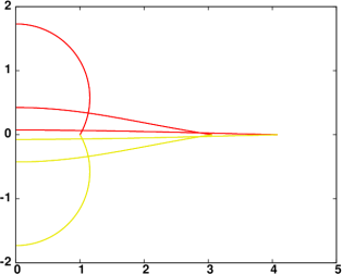
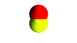
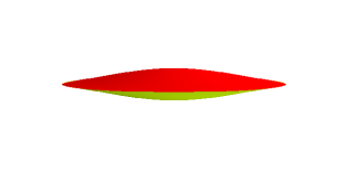
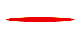
Figure 2: ($C^{0}$) Plots at times $t=0,1,10$.

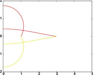
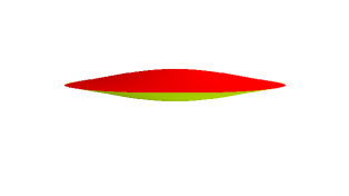
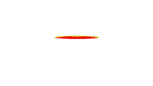
Figure 3: ($C^{0}$: $\varsigma=0.02$) Plots at times $t=0,1,10$.

To conclude this subsection, we show an experiment for phase area and volume conserving flow in Figure 4.

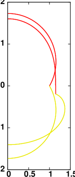
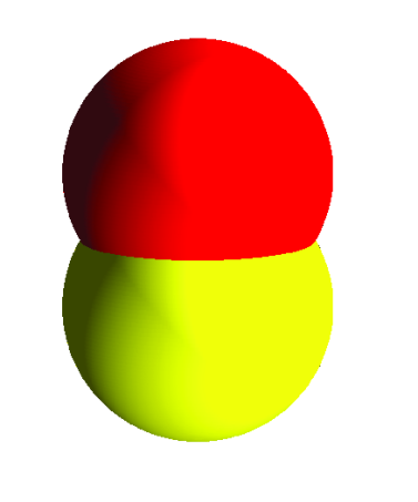
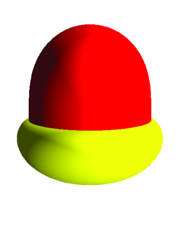
Figure 4: ($C^{0}$ with phase area and volume conservation, ${\overline{\varkappa}}_{1}=-0.5$, ${\overline{\varkappa}}_{2}=-4$) Plots at times $t=0,1$.

In Figure 5 we show a simulation for a flat disc separated into two phases, where phase 2 has two connected components. We note that the model and theory presented in this paper, for simplicity, only considered the case of a single junction being present. But it is a straightforward matter to extend the ideas, and the approximations, to more than one junction. Clearly, in the example in Figure 5 two junctions are present. We let $\Delta t=10^{-4}$ and $(J_{1},J_{2})=(47,84)$.

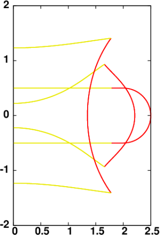
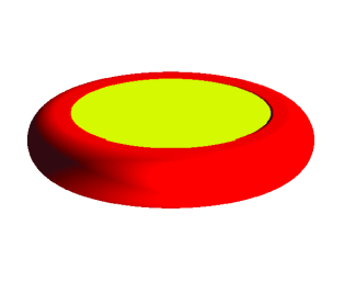
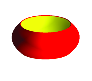
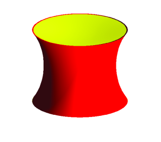
Figure 5: ($C^{0}$ with phase area and volume conservation) Plots at times $t=0,0.1,1$.

6.2 $C^{1}$–junctions

We begin with a study of the tangential motion at the junction, recall Remark 4.5. To this end, we compare the results from our scheme (5.2) to the ones from an alternative fully discrete approximation that is based on (4.8) in place of (4). For the experiments in Figure 6 we start with each phase represented by a quarter of a unit circle. As discretisation parameters we use $\Delta t=10^{-4}$ and $(J_{1},J_{2})=(65,9)$, so that the upper phase is much finer discretised than the lower phase. On the continuous level, the initial data is a steady state solution. However, the scheme based on (4.8) induces a tangential motion of the junction point that is based purely on the discretisation. As a side effect, the whole surface moves up, which is not physical. In contrast, the evolution for our scheme (5.2) is nearly stationary. We note that the condition (4.12) leads to some change at the lower boundary, and we observe a small tangential motion of the junction point.

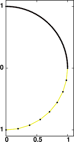
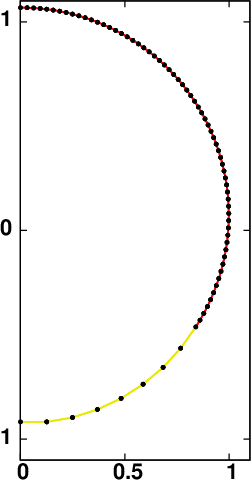
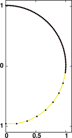
Figure 6: ($C^{1}$) The plots show the initial data (left), the solution of the scheme based on (4.8) at time $t=1$ (middle), and the solution from (5.2) at time $t=1$ (right).

As another comparison, which highlights the rather subtle effects of changing (4) to (4.8), we repeat the experiment in Figure 4, but now for a $C^{1}$–junction with only phase area preservation. As the discretisation parameters we use $J_{1}=J_{2}=65$ and $\Delta t=10^{-4}$. While our scheme (5.2) shows a monotonically decreasing discrete energy, see Figure 7, the fully discrete approximation based on (4.8) exhibits a highly oscillatory energy plot, and some non-trivial tangential motion at the junction point that leads to rather large elements near the junction.

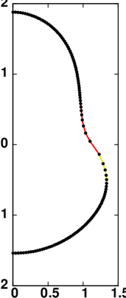
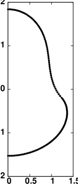
Figure 7: ($C^{1}$ with phase area conservation, ${\overline{\varkappa}}_{1}=-0.5$, ${\overline{\varkappa}}_{2}=-4$) On the left we show the solution at time $t=0.1$, and a plot of the discrete energy, for a fully discrete approximation based on (4.8). On the right we display the same for our scheme (5.2).

This in turn leads to bad curvature approximations at the junction. We visualise this in Figure 8, where for the final solution of both schemes we plot the approximations $\mathfrak{K}^{h}_{i}(\vec{X}^{M}_{i},\kappa^{M}_{i})$ of $\varkappa_{\mathcal{S}_{i}}$, $i=1,2$, against arclength. Clearly, the curvature approximations from the scheme based on (4.8) are completely unphysical. The discretisations from our scheme (5.2), on the other hand , approximately satisfy (2.18a) and (2.18b), which yield $\varkappa_{\mathcal{S}_{1}}-\varkappa_{\mathcal{S}_{2}}=3.5$ and $(\varkappa_{\mathcal{S}_{1}})_{s}=(\varkappa_{\mathcal{S}_{2}})_{s}$, respectively, for the continuous solution at the junction.

Figure 8: ($C^{1}$ with phase area conservation, ${\overline{\varkappa}}_{1}=-0.5$, ${\overline{\varkappa}}_{2}=-4$) A plot of $\mathfrak{K}^{h}_{i}(\vec{X}^{M}_{i},\kappa^{M}_{i})$, $i=1,2$, against arclength of $\overline{\Gamma^{M}_{1}}\cup\overline{\Gamma^{M}_{2}}$, for the two experiments in Figure 7.

Hence, from now on, we only consider simulations for the scheme (5.2). To begin, we perform a convergence experiment for the special case that the two phases have identical physical properties, with ${\overline{\varkappa}}_{1}={\overline{\varkappa}}_{2}={\overline{\varkappa}}=-1$. Then a sphere of radius $R(t)$, where $R(t)$ satisfies

$$R^{\prime}(t)=-\tfrac{{\overline{\varkappa}}}{R(t)}\,(\tfrac{2}{R(t)}+{\overline{\varkappa}})\,,\quad R(0)=1\,,$$ (6.1)

is a solution to (1.9) with $\lambda_{A,1}=\lambda_{A,2}=\lambda_{V}=0$. The nonlinear ODE (6.1) is solved by $R(t)=z(t)-\tfrac{2}{{\overline{\varkappa}}}$, where $z(t)$ is such that $\tfrac{1}{2}\,(z^{2}(t)-z_{0}^{2})-\tfrac{4}{{\overline{\varkappa}}}\,(z(t)-z_{0})+\tfrac{4}{{\overline{\varkappa}}^{2}}\,\ln\tfrac{z(t)}{z_{0}}+{\overline{\varkappa}}^{2}\,t=0$, with $z_{0}=1+\tfrac{2}{{\overline{\varkappa}}}$. We use the solution to (6.1), with ${\overline{\varkappa}}=-1$, and a sequence of approximations for the unit sphere to compute the error

$$\|\Gamma-\Gamma^{h}\|_{L^{\infty}}=\max_{m=1,\ldots,M}\max_{i=1,2}\max_{j=0,\ldots,J_{i}}\left||\vec{X}^{m}_{i}(q_{i,j})|-R(t_{m})\right|$$

over the time interval $[0,T]$, for $T=1$, between the true solution and the discrete solutions for the scheme (5.2). This error only measures the accuracy of the normal motion of the interface, accounting for the fact that the continuous problem has a whole family of solutions, with the tangential motion essentially arbitrary. Nevertheless, in the absence of tangential energetic forcings, any numerical method should ensure that the phase boundary does not move tangentially during the evolution. In order to measure this property, we also compute the quantity $|\vec{X}^{M}(\tfrac{1}{2})-R(T)\,\vec{e}_{1}|$ for the solutions of the scheme (5.2). As initial data we choose $\vec{X}^{0}\in\mathbb{X}^{h}$ with

$$\vec{X}^{0}_{1}(q_{1,j}) =\begin{pmatrix}\cos[(\tfrac{1}{2}-q_{1,j})\,\pi+0.1\,\cos((\tfrac{1}{2}-2\,q_{1,j})\,\pi)]\\ \sin[(\tfrac{1}{2}-q_{1,j})\,\pi+0.1\,\cos((\tfrac{1}{2}-2\,q_{1,j})\,\pi)]\end{pmatrix},\quad j=0,\ldots,J_{1}\,,$$

$$\vec{X}^{0}_{2}(q_{2,j}) =\begin{pmatrix}\cos[(\tfrac{1}{2}-q_{2,j})\,\pi+0.1\,\cos((\tfrac{1}{2}-2\,q_{2,j})\,\pi)]\\ \sin[(\tfrac{1}{2}-q_{2,j})\,\pi+0.1\,\cos((\tfrac{1}{2}-2\,q_{2,j})\,\pi)]\end{pmatrix},\quad j=0,\ldots,J_{2}\,,$$

recall (4.1), which ensures that the evolutions for (5.2) will exhibit some tangential motion within each phase. We use the time step size $\Delta t=10^{-3}\,h^{2}_{\Gamma^{0}}$, where $h_{\Gamma^{0}}$ is the maximal edge length of $\Gamma^{0}=(\Gamma^{0}_{1},\Gamma^{0}_{2})$, and report the computed errors in Table 1. The reported errors appear to indicate an at least linear convergence rate for the two error quantities. We remark that the final element ratios

$$r^{M}_{i}=\dfrac{\max_{j=1,\ldots,J_{i}}|\vec{X}^{M}_{i}(q_{i,j})-\vec{X}^{M}_{i}(q_{i,j-1})|}{\min_{j=1,\ldots,J_{i}}|\vec{X}^{M}_{i}(q_{i,j})-\vec{X}^{M}_{i}(q_{i,j-1})|}\,,\ i=1,2\,,$$

have the value $1$ for each of the runs displayed in Table 1. Of course, this is to be expected from the equidistribution results in Remark 4.5.

$(J_{1}-1,J_{2}-1)$	$h_{\Gamma^{0}}$	$\|\Gamma-\Gamma^{h}\|_{L^{\infty}}$	EOC	$|\vec{X}^{M}(\tfrac{1}{2})-R(T)\,\vec{e}_{1}|$	EOC
(16,8)	2.3408e-01	4.4399e-02	—	3.9101e-02	—
(32,16)	1.1762e-01	1.3277e-02	1.75	1.8489e-02	1.09
(64,32)	5.8881e-02	3.8599e-03	1.79	9.1529e-03	1.02
(128,64)	2.9449e-02	1.0863e-03	1.83	4.5772e-03	1.00
(256,128)	1.4726e-02	3.8711e-04	1.49	2.2921e-03	1.00

Table 1: Errors for the convergence test with ${\overline{\varkappa}}_{1}={\overline{\varkappa}}_{2}=-1$ for the scheme $(\mathcal{P}^{m})^{h}$.

In the next experiments we approximate well-known equilibrium shapes from ?, Fig. 8, see also the experiments in ?, Fig. 7.21. To this end, we consider the volume and phase area conserving flow for initial surfaces with reduced volumes $v_{r}\in\{0.95,\,0.91,\,0.9,\ 0.885,\ 0.84,\ 0.8\}$, where

$$v_{r}=\frac{3\,V(\vec{X}^{0})}{4\,\pi\,(\frac{A_{1}(\vec{X}^{0})+A_{2}(\vec{X}^{0})}{4\,\pi})^{\frac{3}{2}}}=\frac{6\,\pi^{\frac{1}{2}}\,V(\vec{X}^{0})}{(A_{1}(\vec{X}^{0})+A_{2}(\vec{X}^{0}))^{\frac{3}{2}}}\,.$$

In addition, the surface areas are fixed so that $A_{1}(\vec{X}^{0})+A_{2}(\vec{X}^{0})=4\,\pi$ and so that the two phases have a surface area ratio of $\frac{A_{1}(\vec{X}^{0})}{A_{1}(\vec{X}^{0})+A_{2}(\vec{X}^{0})}=0.1$. See Figure 9 for the initial shapes, where the spatial discretisation parameters are given by $(J_{1},J_{2})=(93,421)$, $(91,423)$, $(90,424)$, $(92,422)$, $(95,419)$ and $(97,417)$, respectively. For these experiments we set $\varsigma=9$. Choosing a time step size of $\Delta t=10^{-5}$, we integrate the volume and phase area conserving flow until the discrete energy becomes stationary, and we report on the obtained shapes in Figure 10. These configurations appear to agree well with the computed shapes in ?, Fig. 8.

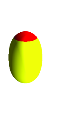
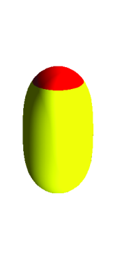
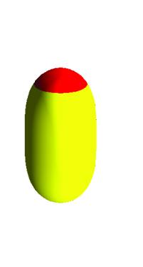
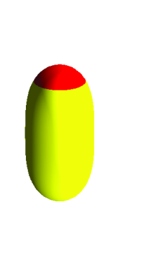
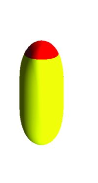
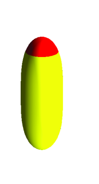
Figure 9: The initial shapes for $v_{r}=0.95$, $0.91$, $0.9$, $0.885$, $0.84$ and $0.8$, respectively.

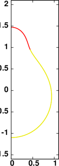
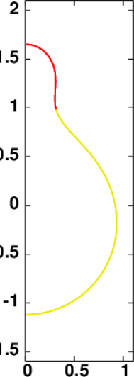
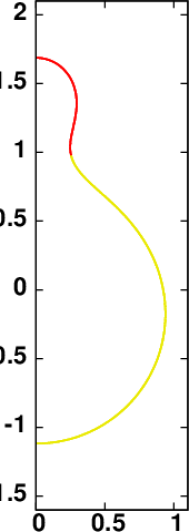
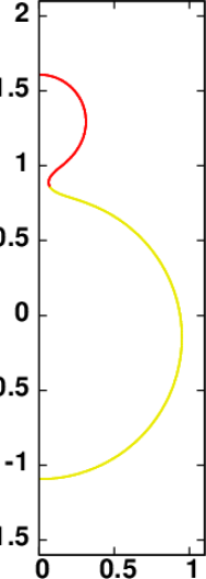
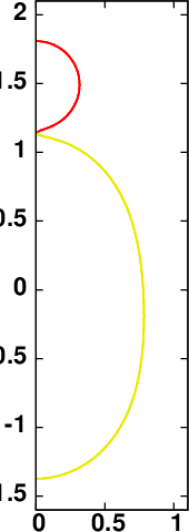
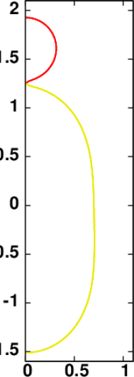
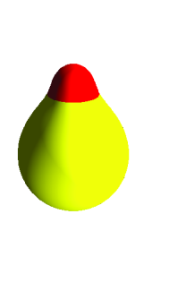
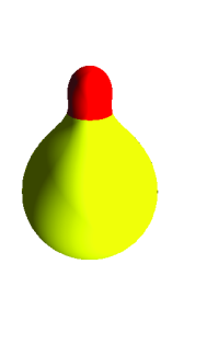
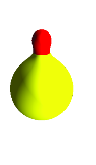
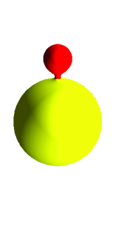
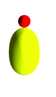
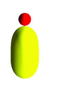
Figure 10: ($C^{1}$ with phase area and volume conservation, $\varsigma=9$) Approximations of the equilibrium shapes for $v_{r}=0.95$, $0.91$, $0.9$, $0.885$, $0.84$ and $0.8$, respectively.

Next we vary the Gaussian bending rigidity $\alpha^{G}_{1}$ for the equilibrium shape in Figure 10 with $v_{r}=0.9$, and report on the new equilibrium shapes in Figure 11. It can clearly be observed, that the interface between the two phases moves away from the neck position, if $|\alpha^{G}_{1}|$ increases. This can be explained with the help of the axisymmetric formulation of the Gaussian curvature contribution in the energy. In fact, in the $C^{1}$–case, when $\vec{\mu}_{2}(\tfrac{1}{2})=-\vec{\mu}_{1}(\tfrac{1}{2})$, we obtain, compare (2.10),

$$2\,\pi\,(\alpha^{G}_{1}-\alpha^{G}_{2})\,\vec{\mu}_{2}(\tfrac{1}{2})\,.\,\vec{e}_{1}$$

as the Gaussian curvature contribution. This implies that the first component of $\vec{\mu}_{2}(\frac{1}{2})$ prefers to be positive if $\alpha_{1}^{G}-\alpha_{2}^{G}<0$, and prefers to be negative if $\alpha_{1}^{G}-\alpha_{2}^{G}>0$. We observe this behaviour in Figure 11, and in particular observe that phase 2 is in the neck region if $\alpha^{G}_{1}$ is negative and phase 1 is in the neck region if $\alpha^{G}_{1}$ is positive, compare also ?, Fig. 5. For the numerical results in Figure 11 we remark that the condition (1.3) is only satisfied if $\alpha^{G}_{1}\in[-2,2]$. Yet also for values outside this interval, our numerical method is able to integrate the evolution, and the movement of the phase boundary becomes ever more pronounced. In addition, we show some equilibrium shapes for $\alpha^{G}_{1}\in[-2,2]$ when the surface has a reduced volume of $v_{r}=0.885$. In this case, we observe an induced pinch-off for $\alpha^{G}_{1}=2$, see Figure 12.

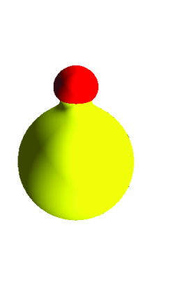
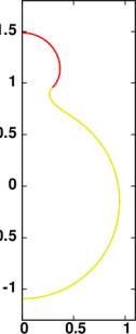
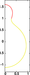
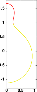
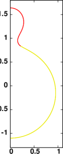
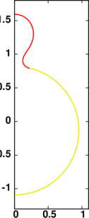
Figure 11: ($C^{1}$ with phase area and volume conservation, $\varsigma=9$) Approximations of the equilibrium shapes for $v_{r}=0.9$, when $\alpha_{1}^{G}=-8,-2,0,2,8$. Apart from the cuts, we also show the surfaces for $\alpha_{1}^{G}=-8$ (left) and for $\alpha_{1}^{G}=8$ (right).

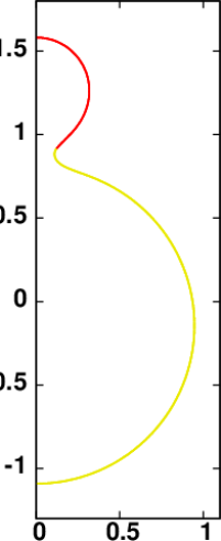
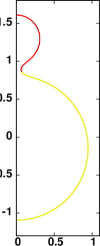
Figure 12: ($C^{1}$ with phase area and volume conservation, $\varsigma=9$) Approximations of the equilibrium shapes for $v_{r}=0.885$, when $\alpha_{1}^{G}=-2,0,2$. Apart from the cuts, we also show the surfaces for $\alpha_{1}^{G}=-2$ (left) and for $\alpha_{1}^{G}=2$ (right). Note that for $\alpha_{1}^{G}=2$ the gradient flow encounters pinch-off.

In the next set of numerical results, we consider the case that one of the phases has two connected components. These results are inspired by the vesicle shapes found in experiments. First we consider a surface with reduced volume $v_{r}=0.956$, total surface area $A_{1}+A_{2}=4\,\pi$ and with a phase area ratio of $A_{1}/(A_{1}+A_{2})=0.46$. Our numerical results in Figure 13 show some resemblance with ?, Fig. 1d, see also ?, Fig. 4.

 

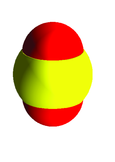
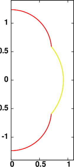
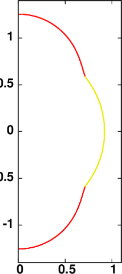
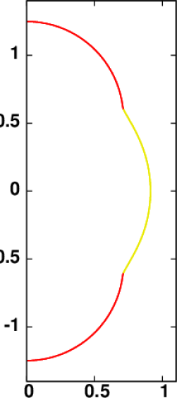
Figure 13: ($C^{1}$ with phase area and volume conservation, $\varsigma=50$) Approximations of the equilibrium shapes for $v_{r}=0.956$. The surface for $(\alpha_{1},\alpha_{2})=(0.01,0.01)$, as well as the cuts for $(\alpha_{1},\alpha_{2})=(0.01,0.01)$ (left), $(\alpha_{1},\alpha_{2})=(1,0.01)$ (middle) and $(\alpha_{1},\alpha_{2})=(0.01,1)$ (right).

Next we consider the shape in ?, Fig. 2f, see also the final simulated surface in ?, Fig. 3. We consider a surface with reduced volume $v_{r}=0.8$, total surface area $A_{1}+A_{2}=4\,\pi$ and with a phase area ratio of $A_{1}/(A_{1}+A_{2})=0.09$. Our numerical results are shown in Figure 14 and the results resemble the situation in the neck region of the experiments of ?, Fig. 2f.

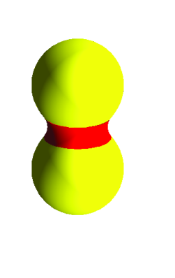
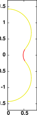
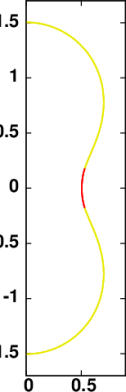
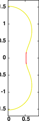
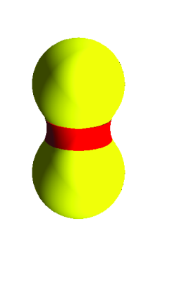
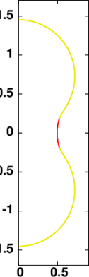
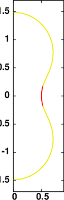
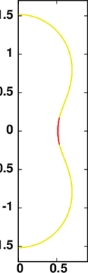
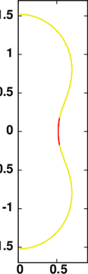
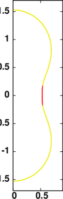
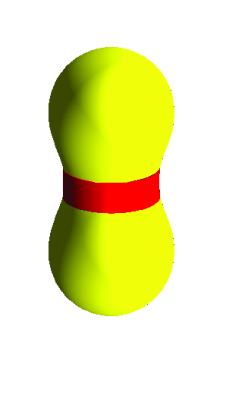
Figure 14: ($C^{1}$ with phase area and volume conservation, $\varsigma=9$) Approximations of the equilibrium shapes for $v_{r}=0.8$, when $(\alpha_{1},\alpha_{2})=(1,0.1)$, $(1,0.5)$, $(1,1)$, $(0.5,1)$, $(0.1,1)$ and ${\overline{\varkappa}}_{1}=2$ (top), as well as for ${\overline{\varkappa}}_{1}=0$ (bottom). On the sides we show the surfaces for $(\alpha_{1},\alpha_{2})=(1,0.1)$ (left) and $(\alpha_{1},\alpha_{2})=(0.1,1)$ (right).

Appendix A Consistency of the weak formulations

Starting from our weak formulations, (3.7) with (3.7a) replaced by (3.1), in this appendix we derive the strong form for the $L^{2}$–gradient flow of (2.11), together with the boundary conditions that need to hold on $\partial I_{i}$, for $i=1,2$. Here we will make extensive use of ?, Appendix A, and for ease of exposition we will often suppress the dependence on time. We begin by writing (3.1) as

$$2\,\pi\,\sum_{i=1}^{2}\left((\vec{x}_{i}\,.\,\vec{e}_{1})\,[\vec{x}_{i}]_{t}\,.\,\vec{\nu}_{i},\vec{\chi}_{i}\,.\,\vec{\nu}_{i}\,|[\vec{x}_{i}]_{\rho}|\right)=\sum_{i=1}^{2}D_{i}(\vec{\chi})\quad\forall\ \vec{\chi}\in\mathbb{X}\,,$$

where

$$D_{i}(\vec{\chi}) =\left([\vec{y}_{i}]_{\rho}\,.\,\vec{\nu}_{i},[\vec{\chi}_{i}]_{\rho}\,.\,\vec{\nu}_{i}\,|[\vec{x}_{i}]_{\rho}|^{-1}\right)+\left(\vec{f}_{i},\vec{\chi}_{i}\,|[\vec{x}_{i}]_{\rho}|\right)-2\,\pi\,\lambda_{V}\left((\vec{x}_{i}\,.\,\vec{e}_{1})\,\vec{\nu}_{i},\vec{\chi}_{i}\,|[\vec{x}_{i}]_{\rho}|\right)$$

$$\quad-2\,\pi\,\lambda_{A,i}\left[\left(\vec{e}_{1},\vec{\chi}_{i}\,|[\vec{x}_{i}]_{\rho}|\right)+\left((\vec{x}_{i}\,.\,\vec{e}_{1})\,\vec{\tau}_{i},[\vec{\chi}_{i}]_{\rho}\right)\right],\ i=1,2\,.$$ (A.1)

On noting that the right hand side of (A.1) corresponds to the right hand side of ?, (A.2) for a single curve, we can apply the results from ?, Appendix A to show that the strong formulations for the flows in the interior are given by (2), while the boundary conditions on $\partial I_{i}\setminus\{\tfrac{1}{2}\}$, for $i=1,2$, are (2.19). Hence it only remains to derive the conditions that need to hold at the junction, i.e. on $\{\tfrac{1}{2}\}$. Collecting the contributions that arise from the boundary terms $B_{1},\ldots,B_{5}$ in ?, Appendix A.1 at the junction point for each of the two curves, which altogether arise from the first, second and last term on the right hand side of (A.1), we obtain that the weak formulation enforces

$$\sum_{i=1}^{2}\left\{(-1)^{i+1}([\vec{y}_{i}]_{s}\,.\,\vec{\nu}_{i})\,\vec{\chi}_{i}\,.\,\vec{\nu}_{i}-\pi\,\varsigma\,\vec{\chi}_{i}\,.\,\vec{e}_{1}-\pi\,(-1)^{i+1}\,\vec{x}_{i}\,.\,\vec{e}_{1}\,(\alpha_{i}\,[\varkappa_{\mathcal{S}_{i}}-{\overline{\varkappa}}_{i}]^{2}+2\,\lambda_{A,i})\,\vec{\chi}_{i}\,.\,\vec{\tau}_{i}\right.$$

$$\qquad\left.-2\,\pi\,\alpha_{i}\,(-1)^{i+1}\,(\varkappa_{\mathcal{S}_{i}}-{\overline{\varkappa}}_{i})\,(\vec{\tau}_{i}\,.\,\vec{e}_{1})\,\vec{\chi}_{i}\,.\,\vec{\nu}_{i}+(-1)^{i+1}\left[\varkappa_{i}\,\vec{\chi}_{i}\,.\,\vec{y}_{i}^{\perp}\right]\right\}=0$$ (A.2)

at the junction. We note from (3.6) and (2.4) that

$$\vec{y}_{i}\,.\,\vec{\nu}_{i}=2\,\pi\,\vec{x}_{i}\,.\,\vec{e}_{1}\,\alpha_{i}\,(\varkappa_{\mathcal{S}_{i}}-{\overline{\varkappa}}_{i})\,,\quad\text{where}\quad\varkappa_{\mathcal{S}_{i}}=\varkappa_{i}-\frac{\vec{\nu}_{i}\,.\,\vec{e}_{1}}{\vec{x}_{i}\,.\,\vec{e}_{1}}\quad\text{in }\overline{I}_{i}\,,\ i=1,2\,.$$ (A.3)

Moreover, we recall from ?, (3.24) that it can be shown that

$$\varkappa_{i}\,\vec{y}_{i}^{\perp}+([\vec{y}_{i}]_{s}\,.\,\vec{\nu}_{i})\,\vec{\nu}_{i}=\varkappa_{i}\,(\vec{y}_{i}\,.\,\vec{\nu}_{i})\,\vec{\tau}_{i}+(\vec{y}_{i}\,.\,\vec{\nu}_{i})_{s}\,\vec{\nu}_{i}\quad\text{in }\overline{I}_{i}\,,\ i=1,2\,.$$ (A.4)

It follows from (A.4) and (A.3) that we can combine the first and last term on the left hand side of (A.2) to give

$$2\,\pi\,\sum_{i=1}^{2}(-1)^{i+1}\left\{\varkappa_{i}\,\vec{x}_{i}\,.\,\vec{e}_{1}\,\alpha_{i}\,(\varkappa_{\mathcal{S}_{i}}-{\overline{\varkappa}}_{i})\,\vec{\chi}_{i}\,.\,\vec{\tau}_{i}+\alpha_{i}\,[\vec{x}_{i}\,.\,\vec{e}_{1}\,(\varkappa_{\mathcal{S}_{i}})_{s}+\vec{\tau}_{i}\,.\,\vec{e}_{1}\,(\varkappa_{\mathcal{S}_{i}}-{\overline{\varkappa}}_{i})]\,\vec{\chi}_{i}\,.\,\vec{\nu}_{i}\right\}.$$

Hence, on using the notations $\vec{x}=\vec{x}_{1}=\vec{x}_{2}$ and $\vec{\chi}=\vec{\chi}_{1}=\vec{\chi}_{2}$ at the point $\frac{1}{2}$, and on recalling (2.9), it follows from (A.2) that

$$2\,\pi\,\vec{x}\,.\,\vec{e}_{1}\,\sum_{i=1}^{2}\left[(-1)^{i+1}\,\alpha_{i}\,(\varkappa_{\mathcal{S}_{i}})_{s}\,\vec{\nu}_{i}-(\tfrac{1}{2}\,\alpha_{i}\,(\varkappa_{\mathcal{S}_{i}}-{\overline{\varkappa}}_{i})^{2}+\lambda_{A,i})\,\vec{\mu}_{i}+\alpha_{i}\,(\varkappa_{\mathcal{S}_{i}}-{\overline{\varkappa}}_{i})\,\varkappa_{i}\,\vec{\mu}_{i}\right.$$

$$\qquad\qquad\left.-\tfrac{1}{2}\,\frac{\varsigma}{\vec{x}\,.\,\vec{e}_{1}}\,\vec{e}_{1}\right].\,\vec{\chi}=0\,.$$

As $\vec{\chi}\in\mathbb{X}$ is arbitrary, we obtain from the above identity that

$$\sum_{i=1}^{2}\left[(-1)^{i+1}\,\alpha_{i}\,(\varkappa_{\mathcal{S}_{i}})_{s}\,\vec{\nu}_{i}-(\tfrac{1}{2}\,\alpha_{i}\,(\varkappa_{\mathcal{S}_{i}}-{\overline{\varkappa}}_{i})^{2}+\lambda_{A,i}-\alpha_{i}\,(\varkappa_{\mathcal{S}_{i}}-{\overline{\varkappa}}_{i})\,\varkappa_{i})\,\vec{\mu}_{i}\right]-\frac{\varsigma}{\vec{x}\,.\,\vec{e}_{1}}\,\vec{e}_{1}$$

$$\qquad=\vec{0}\quad\text{on }\overline{I}_{1}\cap\overline{I}_{2}\,.$$ (A.5)

We first consider the case of a $C^{0}$–junction, i.e. $C_{1}=0$. Then it follows from (3.7d) and (A.3) that

$$\alpha_{i}\,(\varkappa_{\mathcal{S}_{i}}-{\overline{\varkappa}}_{i})=\alpha_{i}^{G}\,\frac{\vec{\nu}_{i}\,.\,\vec{e}_{1}}{\vec{x}\,.\,\vec{e}_{1}}\quad\text{on }\partial I_{i}\setminus\{0,1\}\,,\ i=1,2\,,$$

which is (2.17a). Using this identity in (A.5), we obtain with the help of (2.4) that

$$\sum_{i=1}^{2}\left[(-1)^{i+1}\,\alpha_{i}\,(\varkappa_{\mathcal{S}_{i}})_{s}\,\vec{\nu}_{i}-(\tfrac{1}{2}\,\alpha_{i}\,(\varkappa_{\mathcal{S}_{i}}-{\overline{\varkappa}}_{i})^{2}+\lambda_{A,i}+\alpha_{i}^{G}\,{\mathcal{K}}_{\mathcal{S}_{i}})\,\vec{\mu}_{i}\right]-\frac{\varsigma}{\vec{x}\,.\,\vec{e}_{1}}\,\vec{e}_{1}=\vec{0}\,,$$

which is (2.17b). This shows that the weak formulation implies the boundary conditions at the junction in the $C^{0}$–case.

In the $C^{1}$–case, i.e. for $C_{1}=1$, we recall from Remark 3.1 that

$$\vec{y}_{1}-\vec{y}_{2}=2\,\pi\,[\alpha_{1}^{G}-\alpha_{2}^{G}]\,\vec{e}_{1}\quad\text{on }\overline{I}_{1}\cap\overline{I}_{2}\,,$$ (A.6)

and that (3.8) holds. Applying integration by parts to the two second order terms in (3.8), and observing the fact that $\vec{\eta}_{1}(\tfrac{1}{2})=\vec{\eta}_{2}(\tfrac{1}{2})$ as $(\vec{\eta}_{1},\vec{\eta}_{2})\in\mathbb{Y}_{C^{1}}$, yields

$$\frac{[\vec{x}_{1}]_{\rho}}{|[\vec{x}_{1}]_{\rho}|}-\frac{[\vec{x}_{2}]_{\rho}}{|[\vec{x}_{2}]_{\rho}|}=\vec{0}\quad\text{ on }\overline{I}_{1}\cap\overline{I}_{2}\,,$$

which, on using (2.2) and (2.9), implies that

$$\vec{\nu}:=\vec{\nu}_{2}=\vec{\nu}_{1}\quad\text{ and }\quad\vec{\mu}:=\vec{\mu}_{2}=-\vec{\mu}_{1}\quad\text{ on }\overline{I}_{1}\cap\overline{I}_{2}\,.$$ (A.7)

On combining (A.6) and (3.7b), which states that $2\,\pi\,\alpha_{i}\,\vec{x}_{i}\,.\,\vec{e}_{1}\,(\varkappa_{\mathcal{S}_{i}}-{\overline{\varkappa}}_{i})=\vec{y}_{i}\,.\,\vec{\nu}_{i}$ in $\overline{I}_{i}$, we obtain, on recalling the first definition in (A.7), that

$$[\alpha_{i}\,(\varkappa_{\mathcal{S}_{i}}-{\overline{\varkappa}}_{i})]^{2}_{1}-[\alpha_{i}^{G}]^{2}_{1}\,\frac{\vec{\nu}\,.\,\vec{e}_{1}}{\vec{x}\,.\,\vec{e}_{1}}=0\quad\text{ on }\overline{I}_{1}\cap\overline{I}_{2}\,,$$

which is (2.18a). Moreover, substituting (A.7) into (A.5) gives

$$\sum_{i=1}^{2}(-1)^{i+1}\left[\alpha_{i}\,(\varkappa_{\mathcal{S}_{i}})_{s}\,\vec{\nu}+(\tfrac{1}{2}\,\alpha_{i}\,(\varkappa_{\mathcal{S}_{i}}-{\overline{\varkappa}}_{i})^{2}+\lambda_{A,i}-\alpha_{i}\,(\varkappa_{\mathcal{S}_{i}}-{\overline{\varkappa}}_{i})\,\varkappa_{i})\,\vec{\mu}\right]-\frac{\varsigma}{\vec{x}\,.\,\vec{e}_{1}}\,\vec{e}_{1}=\vec{0}$$

at the junction, and taking the inner products with $\vec{\nu}$ and $\vec{\mu}$ leads to

$$-[\alpha_{i}\,(\varkappa_{\mathcal{S}_{i}})_{s}]^{2}_{1}-\varsigma\,\frac{\vec{\nu}\,.\,\vec{e}_{1}}{\vec{x}\,.\,\vec{e}_{1}}=0\quad\text{on }\overline{I}_{1}\cap\overline{I}_{2}$$

and

$$[-\tfrac{1}{2}\,\alpha_{i}\,(\varkappa_{\mathcal{S}_{i}}-{\overline{\varkappa}}_{i})^{2}+\alpha_{i}\,(\varkappa_{\mathcal{S}_{i}}-{\overline{\varkappa}}_{i})\,\varkappa_{i}-\lambda_{A,i}]^{2}_{1}-\varsigma\,\frac{\vec{\mu}\,.\,\vec{e}_{1}}{\vec{x}\,.\,\vec{e}_{1}}=0\quad\text{on }\overline{I}_{1}\cap\overline{I}_{2}\,.$$

The last two equations coincide with (2.18b) and (2.18c), respectively. Hence we have shown that in the $C^{1}$–case, the weak formulation implies the correct boundary conditions (2.18).

Appendix B Some axisymmetric differential geometry

In this appendix, we review some material on the geometry of surfaces from Chapter 2 in the recent review article ?, and apply it to axisymmetric surfaces.

Let $\vec{x}:I\to{\mathbb{R}}^{2}$, $I\subset{\mathbb{R}}$, be a local parameterisation of the curve $\Gamma$, with tangent $\vec{\tau}=|\vec{x}_{\rho}|^{-1}\,\vec{x}_{\rho}=\vec{x}_{s}$, unit normal $\vec{\nu}$ and curvature vector $\varkappa\,\vec{\nu}=\vec{\tau}_{s}$, where we have defined $\partial_{s}=|\vec{x}_{\rho}|^{-1}\,\partial_{\rho}$. Let $\Gamma$ be the generating curve of an axisymmetric surface $\mathcal{S}$ in ${\mathbb{R}}^{3}$. Then $\vec{y}:I\times[0,2\,\pi)\to{\mathbb{R}}^{3}$ is a local parameterisation of $\mathcal{S}$, where

$$\vec{y}(\rho,\theta)=(\vec{x}(\rho)\,.\,\vec{e}_{1}\,\cos\theta,\vec{x}(\rho)\,.\,\vec{e}_{2},\vec{x}(\rho)\,.\,\vec{e}_{1}\,\sin\theta)^{T}\,.$$

The tangent space of $\mathcal{S}$ at $\vec{y}(\rho,\theta)$ is spanned by the two tangent vectors

$$\vec{y}_{\rho}(\rho,\theta) =|\vec{x}_{\rho}|\,(\vec{\tau}\,.\,\vec{e}_{1}\,\cos\theta,\vec{\tau}\,.\,\vec{e}_{2},\vec{\tau}\,.\,\vec{e}_{1}\,\sin\theta)^{T}\,,$$

$$\vec{y}_{\theta}(\rho,\theta) =(-\vec{x}\,.\,\vec{e}_{1}\,\sin\theta,0,\vec{x}\,.\,\vec{e}_{1}\,\cos\theta)^{T}\,,$$ (B.1)

and a unit normal vector can be defined via

$$\vec{\nu}_{\mathcal{S}}(\rho,\theta)=(\vec{\nu}\,.\,\vec{e}_{1}\,\cos\theta,\vec{\nu}\,.\,\vec{e}_{2},\vec{\nu}\,.\,\vec{e}_{1}\,\sin\theta)^{T}\,.$$ (B.2)

It follows from (B) and ?, Remark 8 that the coefficients of the first fundamental form of $\mathcal{S}$ are given by

$$g_{\rho\rho}=|\vec{y}_{\rho}|^{2}=|\vec{x}_{\rho}|^{2}\,,\quad g_{\theta\theta}=|\vec{y}_{\theta}|^{2}=(\vec{x}\,.\,\vec{e}_{1})^{2}\,,\quad g_{\rho\theta}=g_{\theta\rho}=\vec{y}_{\rho}\,.\,\vec{y}_{\theta}=0\,,$$ (B.3)

with the square of the local area element on $\mathcal{S}$ given by

$$g=g_{\theta\theta}\,g_{\rho\rho}=(\vec{x}\,.\,\vec{e}_{1})^{2}\,|\vec{x}_{\rho}|^{2}\quad\text{in }I\times[0,2\,\pi)\,.$$ (B.4)

Moreover, it follows from (B.3) and ?, Remark 8 that the surface gradient and the surface divergence of smooth functions $f:\mathcal{S}\to{\mathbb{R}}$, $\vec{f}:\mathcal{S}\to{\mathbb{R}}^{3}$ on $\mathcal{S}$ can be calculated as

$$(\nabla_{\!\mathcal{S}}\,f)\circ\vec{y} =|\vec{y}_{\rho}|^{-2}\,(f\circ\vec{y})_{\rho}\,\vec{y}_{\rho}+|\vec{y}_{\theta}|^{-2}\,(f\circ\vec{y})_{\theta}\,\vec{y}_{\theta}$$

$$=(f\circ\vec{y})_{s}\,\vec{y}_{s}+(\vec{x}\,.\,\vec{e}_{1})^{-2}\,(f\circ\vec{y})_{\theta}\,\vec{y}_{\theta} \quad\text{in }I\times[0,2\,\pi)\,,$$

$$(\nabla_{\!\mathcal{S}}\,.\,\vec{f})\circ\vec{y} =(\vec{f}\circ\vec{y})_{s}\,.\,\vec{y}_{s}+(\vec{x}\,.\,\vec{e}_{1})^{-2}\,(\vec{f}\circ\vec{y})_{\theta}\,.\,\vec{y}_{\theta} \quad\text{in }I\times[0,2\,\pi)\,.$$

Hence, on noting $((\vec{x}\,.\,\vec{e}_{1})^{-1}\,\vec{y}_{\theta})_{s}=\vec{0}$ and $(\vec{y}_{s})_{\theta}\,.\,\vec{y}_{\theta}=(\vec{x}\,.\,\vec{e}_{1})\,\vec{x}_{s}\,.\,\vec{e}_{1}$, we obtain that

$$(\Delta_{\mathcal{S}}\,f)\circ\vec{y} =(\nabla_{\!\mathcal{S}}\,.\,(\nabla_{\!\mathcal{S}}\,f))\circ\vec{y}$$

$$=(f\circ\vec{y})_{ss}+\frac{\vec{x}_{s}\,.\,\vec{e}_{1}}{\vec{x}\,.\,\vec{e}_{1}}\,(f\circ\vec{y})_{s}+(\vec{x}\,.\,\vec{e}_{1})^{-2}\,(f\circ\vec{y})_{\theta\theta} \quad\text{in }I\times[0,2\,\pi)\,.$$

For a radially symmetric function $f:\mathcal{S}\to{\mathbb{R}}$, with $f(\vec{y}(\rho,\theta))=f(\vec{y}(\rho,0))$ for all $(\rho,\theta)\in I\times[0,2\,\pi)$, it follows that

$$(\Delta_{\mathcal{S}}\,f)\circ\vec{y}=(\vec{x}\,.\,\vec{e}_{1})^{-1}\,(\vec{x}\,.\,\vec{e}_{1}\,(f\circ\vec{y})_{s})_{s}\quad\text{in }I\times[0,2\,\pi)\,.$$ (B.5)

On recalling Definitions 10 and 11 in ?, we now compute the principal curvatures of $\mathcal{S}$ as the eigenvalues of the Weingarten map $W_{\vec{p}}(\vec{\mathfrak{t}})=-\partial_{\vec{\mathfrak{t}}}\,\vec{\nu}_{\mathcal{S}}$ at $\vec{p}=\vec{y}(\rho,\theta)$. Choosing for the tangent vector $\vec{\mathfrak{t}}$ the first vector in (B), recalling (B.2), and noting that $\partial_{\vec{y}_{\rho}}=\partial_{\rho}$, we obtain

$$W_{\vec{p}}(\vec{y}_{\rho})=-\partial_{\vec{y}_{\rho}}\,\vec{\nu}_{\mathcal{S}} =-[\vec{\nu}_{\mathcal{S}}]_{\rho}=-|\vec{x}_{\rho}|\,[\vec{\nu}_{\mathcal{S}}]_{s}=-|\vec{x}_{\rho}|(\vec{\nu}_{s}\,.\,\vec{e}_{1}\,\cos\theta,\vec{\nu}_{s}\,.\,\vec{e}_{2},\vec{\nu}_{s}\,.\,\vec{e}_{1}\,\sin\theta)^{T}$$

$$=|\vec{x}_{\rho}|\varkappa\,(\vec{\tau}\,.\,\vec{e}_{1}\,\cos\theta,\vec{\tau}\,.\,\vec{e}_{2},\vec{\tau}\,.\,\vec{e}_{1}\,\sin\theta)^{T}=\varkappa\,\vec{y}_{\rho}\,,$$ (B.6a)

where we have used that $$\vec{\nu}_{s}=-\varkappa\,\vec{\tau} \vec{\nu}_{s}\,.\,\vec{\tau}=-\varkappa \vec{\nu}_{s}\,.\,\vec{\nu}=0 \vec{\mathfrak{t}} \partial_{\vec{y}_{\theta}}=\partial_{\theta}$$, since and . Similarly, choosing for the tangent vector the second vector in (B), and noting that , yields

$$W_{\vec{p}}(\vec{y}_{\theta}) =-[\vec{\nu}_{\mathcal{S}}]_{\theta}=-(-\vec{\nu}\,.\,\vec{e}_{1}\,\sin\theta,0,\vec{\nu}\,.\,\vec{e}_{1}\,\cos\theta)^{T}=-\frac{\vec{\nu}\,.\,\vec{e}_{1}}{\vec{x}\,.\,\vec{e}_{1}}\,\vec{y}_{\theta}\,.$$ (B.6b)

Clearly, (B.6) implies that the two eigenvalues of the Weingarten map are $\varkappa$ and $-\frac{\vec{\nu}\,.\,\vec{e}_{1}}{\vec{x}\,.\,\vec{e}_{1}}$, which means that for the mean and Gaussian curvatures of $\mathcal{S}$ we obtain the formulas

$$\varkappa_{\mathcal{S}}=\varkappa-\frac{\vec{\nu}\,.\,\vec{e}_{1}}{\vec{x}\,.\,\vec{e}_{1}}\quad\text{and}\quad{\mathcal{K}}_{\mathcal{S}}=-\varkappa\,\frac{\vec{\nu}\,.\,\vec{e}_{1}}{\vec{x}\,.\,\vec{e}_{1}}\quad\text{in }\ I\times[0,2\,\pi)\,.$$ (B.7)