Metastability in the Potts model:
exact results in the large $q$ limit

Abstract

We study the metastable equilibrium properties of the two dimensional Potts model with heat-bath transition rates using a novel expansion. The method is especially powerful for large number of state spin variables and it is notably accurate in a rather wide range of temperatures around the phase transition.

1 Introduction

The Potts model [1] is an extension of the celebrated ferromagnetic Ising model. In this variation, the spin variables take $q$ integer values (often associated to colours) and are coupled in a way that favours alignment, that is to say, equal values of the spins (colours) placed on neighbouring sites on a lattice. The model attracted attention at the early ages of phase transition studies since the order of the phase transition changes when the number of states of the spins is tuned: in two dimensions, for $2\leq q\leq 4$ it is of second-order, while for $q>4$ it is of first-order [2, 3] with the associated metastability properties. Beyond the fundamental interest that it produced, the Potts model found applications in many areas of physics, and even beyond the physical domain. For instance, the large $q$ limit is used to describe soap foams and metallic grain systems [4, 5, 6]. In its anti-ferromagnetic version, the Potts model represents the colouring problem of computer science [7, 8]. Another application in this realm is to community detection in complex networks [9, 10, 11]. Furthermore, weakly disordered Potts ferromagnets are the paradigmatic models in which the effects of randomness on phase transitions were studied [12, 13], and disordered and frustrated mean-field Potts models [14, 15] realise the random first-order phase transitions scenario for the glassy arrest [16, 17, 18].

The first order transition of the ferromagnetic two dimensional Potts model with $q>4$ is accompanied by metastability properties (with finite life-time in finite dimensions). In general, quantifying metastability and the dynamic escape from it through nucleation is a hard and longstanding problem [19, 20, 21, 22]. In this paper we address metastability in the stochastic bidimensional Potts model with $q>4$ from a novel perspective, that is, by solving the microscopic dynamics in the large $q$ limit. Indeed, in the stochastic model the dynamic evolution proceeds via a Markov Chain with microscopic rules that we have the freedom to choose, conditioned to respect detailed balance. As we argue below, the dynamics are faster, and also easier to understand analytically, when the heat bath microscopic updates are used. This is the rule that we adopt. The choice of initial conditions and working temperature decides the kind of metastability one accesses with the dynamic protocol. More precisely, for sub-critical quenches, in which we follow the evolution of a disordered initial state under conditions in which the system should order ferromagnetically, the metastable state is disordered. Instead, in the opposite quench, in which we prepare the system in a ferromagnetic state and we heat it above the critical point, the metastable state is ferromagnetically ordered. In this paper we consider both kinds of instantaneous quenches. After identifying the (few) relevant microscopic transition paths in the large $q$ limit, we derive the free-energy densities of the two phases and from them various thermodynamic observables that allow us to quantify the metastable behaviour in full detail. We confirm our analytical predictions with numerical simulations of excellent accuracy.

The paper is organised as follows. In Sec. 2 we recall the definition and main properties of the Potts model. In Sec. 3 we introduce the heat bath dynamics, we identify all relevant moves for $q>4$, and we derive the transition probabilities in terms of local configurations updates. Next, Sec. 4 and Sec. 5 describe our results for subcritical and supercritical quenches, respectively. A concluding Section closes our work.

2 The model

The Potts model [1] is defined by the energy function

$$H_{J}[\{s_{i}\}]=-J\sum_{\langle ij\rangle}\delta_{s_{i}s_{j}}\;,$$ (1)

where $J>0$ is a coupling constant, the sum is restricted to nearest-neighbours on a lattice, $\delta_{ab}$ is the Kronecker delta and $s_{i}$ take integer values from 1 to $q\geq 2$. This model is a generalisation of the Ising model, to which it reduces for $q=2$. There is no external field applied. We will focus on the bidimensional case, defined on an $L\times L$ square lattice with periodic boundary conditions. In the sum one counts each bond once and for this geometry the energy is bounded between $-2JN$, with $N$ the number of spins in the sample, and $0$.

Although the problem is not fully solvable for $q>2$, some exact results are known. Duality allows one to prove that the critical temperature is [1]

$$k_{B}T_{c}(q)=\frac{J}{\ln\left(1+\sqrt{q}\right)}\;.$$ (2)

Henceforth we will set $k_{B}=J=1$.

An exact solution on the square lattice was provided in 1973: by exploiting a mapping to the ice-rule six-vertex model R. J. Baxter gave an exact expression for the model’s free-energy at the critical point. He thus showed that the transition is second order for $q\leq 4$ and first order for $q>4$, and he calculated the latent heat in the latter case [23]. A proof that the simplest possible mean-field approach yields, in the thermodynamic limit, the exact free-energy at criticality for $q\geq q_{c}(d)$ (with $q_{c}(2)=4$) to leading order in $q$, in the large $q$ limit, was soon after given by Mittal & Stephen [24], see also [25]. Many numerical studies put these ideas to the test since then. For example, Binder in Ref. [26] and much more recently the authors of Refs. [27, 28, 29, 30] focused on the analysis of the critical properties, both in the second order and first order cases, using different numerical methods.

In order to go beyond the critical point results, F. Y. Wu exploited a fancy mapping onto a pure math problem to derive the free-energy density in the large $q$ limit at any $T$ (assuming that large $q$ and large $N$ limits commute) [31] and he recovered the already known form at $T_{c}$ [23, 24] as a particular case. More recently, Johansson and Pistol used a microcanonical approach to argue that the entropy per site is given by [32]

$$s(e)=\left(1+\frac{e}{2}\right)\ln q$$ (3)

with $e$ the energy density, in the large $N$ and $q$ limits, irrespectively of the order in which these are taken. They then used this result to calculate the partition function and from it the free-energy density

$$-\beta f\sim\left\{\begin{array}[]{l}\ln q\\ 2\beta\end{array}\right.\qquad\mbox{for}\qquad\left\{\begin{array}[]{l}\beta\ll\beta_{c}\\ \beta\gg\beta_{c}\end{array}\right.\qquad\mbox{with}\quad\beta_{c}\simeq\ln\sqrt{q}$$ (8)

(in the last expression $-\beta f\simeq-\beta e\simeq 2\beta$ for large $\beta$ was used) that coincides with the one found in [31]).

3 Heat bath dynamics

Classical spin models coupled to heat baths evolve in time stochastically according to some microscopic updates that have to be provided to make their definition complete. Concretely, at each microscopic time step ones chooses one site at random and changes the value of the local spin according to some probabilistic rule. For a system with $N$ spins, conventionally, $N$ update attempts correspond to one Monte Carlo step (MCs). In this Section we define the Heat Bath microscopic rule, we enumerate all possible updates of a chosen spin according to its surrounding configurations, and we derive the transition probability for each of them.

3.1 Microscopic rules

The usual microscopic dynamics used in Monte Carlo simulations of spin models are the Metropolis ones, in which one tries to change the spin to a new value (chosen at random among the remaining $q-1$ possibilities) and the move i) is accepted if the new local energy $e_{i}^{\prime}$ is lower than the previous local energy $e_{i}$ or, otherwise, ii) it is accepted with probability $\exp(-\beta(e^{\prime}_{i}-e_{i}))$.

However, in the case of the Potts model, especially in its large $q$ limit, another rule also respecting detailed balance, the so-called heat bath rule, is more efficient and allows for a partial analytic treatment, similarly to what found in other ferromagnetic models [33]. In short, with this rule the transition probabilities are proportional to $e^{-\beta e^{\prime}}$. Specifically, the scheme works as follows. First, one considers the weight associated to each possible value that a spin, say $s_{i}$, can take depending on its local environment. As an example, assume that $s_{i}$ is surrounded, on the square lattice, by two spins taking the value $1$, a spin with value $2$ and another one with value $3$. We attribute the weights $w_{i}(s_{i}=1)=e^{2\beta}$, corresponding to the fact that the spin $i$ taking the value $1$ yields a local energy of $-2$, $w_{i}(s_{i}=2)=e^{\beta}=w_{i}(s_{i}=3)$ because of the local energy being equal to $-1$ in these cases, and $w_{i}(s_{i}=j)=1$ for $3<j\leq q$ for similar reasons. Next, we normalize the $w_{i}$ and we define the probabilities

$$P_{i}(s_{i}=k)=\frac{w_{i}(s_{i}=k)}{\sum_{l=1}^{q}w_{i}(s_{i}=l)}\;.$$ (9)

Having attributed probabilities to the state of the central spin, we can now evaluate the transition probabilities for its update. Imagine that the spin $s_{i}$ takes the value $1$. Then, we choose a random number $r\in[0:1]$. If $r<P_{i}(1)$, the spin keeps its value $s_{i}=1$. Otherwise, if $r<P_{i}(1)+P_{i}(2)$, $s_{i}$ takes the new value $s_{i}=2$, or if $r<P_{i}(1)+P_{i}(2)+P_{i}(3)$, it is updated to $s_{i}=3$, and so on and so forth. Thus, we have the following transition probabilities for the spin $s_{i}=1$ surrounded by two spins $1$, one spin $2$ and one spin $3$:

$$T^{\rm HB}_{1\to 1}=\frac{e^{2\beta}}{e^{2\beta}+2e^{\beta}+q-3}\;,\qquad T^{\rm HB}_{1\to 2}=T^{\rm HB}_{1\to 3}=\frac{e^{\beta}}{e^{2\beta}+2e^{\beta}+q-3}\;,$$ (10)

$$T^{\rm HB}_{1\to j}=\frac{1}{e^{2\beta}+2e^{\beta}+q-3}\;,$$ (11)

with $j$ indicating any possible state with $j>3$ (there are $q-3$ such states). Notice that these probabilities do not depend on the initial state of the spin. Despite this, we prefer to use the notation above to make the comparison with the Metropolis probabilities (Eq. (12)). Proceeding in a similar way one can evaluate the transition probability of any spin, according to its state and the ones of its neighbours.

For the sake comparison, we recall the transition probabilities of the Metropolis rule:

$$T^{\rm M}_{1\to 1}=1-\frac{1}{q-1}(2e^{-\beta}+(q-3)e^{-2\beta})\;,\qquad T^{\rm M}_{1\to 2}=T^{\rm M}_{1\to 3}=\frac{1}{q-1}e^{-\beta}\;,$$

$$T^{\rm M}_{1\to j}=\frac{1}{q-1}e^{-2\beta}\;,$$ (12)

for the same example considered above.

In practice, we find that the heat-bath dynamics are much more efficient, in the sense that the approach to equilibrium is faster, in particular for large $q$. We only consider the heat-bath dynamics in the following.

3.2 Enumeration

For any integer $q\geq 5$ we can classify all local configurations, seen as vertices with a central spin and its four first neighbours, and identify all possible updates. The method goes like this. Take one spin $s_{i}$, count the number of neighbouring spins with the same value as the selected central one, and call this number $n_{1}$. Next, count the number of neighbours with the most present spin value different from the central one and call this number $n_{2}$. Continue in this way and organise these numbers in decreasing order, that is, $n_{1},\,n_{2},\,n_{3},\dots$. It is easy to see that, with this classification, there are only 11 local configurations (we do not distinguish which are the neighbours that take the same or different values as the central one) and they are represented in the figure below:


     

     

     

In the following we will use the name “sand” to refer to the configurations (11) in which all sites take different values. We now use a more detailed notation to identify each of these configurations writing explicitly the number of neighbours of each kind, that is to say, using $[n_{1},n_{2},\dots]$ where only the values $n_{i}\neq 0$ are kept. Proceeding in this way we have

$$(0) : [4]\rightarrow(0)\;,\;(7)$$

$$(1) : [3,1]\rightarrow(1)\;,\;(4)\;,\;(8)$$

$$(2) : [2,2]\rightarrow(2)\;,\;(2)\;,\;(9)$$

$$(3) : [2,1,1]\rightarrow(3)\;,\;(5)\;,\;(10)$$

$$(4) : [1,3]\rightarrow(4)\;,\;(1)\;,\;(8)$$

$$(5) : [1,2,1]\rightarrow(5)\;,\;(3)\;,\;(10)$$

$$(6) : [1,1,1,1]\rightarrow(6)\;,\;(11)$$

$$(7) : [0,4]\rightarrow(7)\;,\;(0)$$

$$(8) : [0,3,1]\rightarrow(8)\;,\;(1)\;,\;(4)$$

$$(9) : [0,2,2]\rightarrow(9)\;,\;(2)$$

$$(10) : [0,2,1,1]\rightarrow(10)\;,\;(3)\;,\;(5)$$

$$(11) : [0,1,1,1,1]\rightarrow(11)\;,\;(6)$$

where the right arrows and the values after them indicate the transitions generated by the update of the central spin. For example, the first configuration, denoted by $(0)$, can either keep the same value, thus the $(0)$ on the right, or take another value, thus the configuration $(7):[0,4]$. Again, this should be easy to grasp by looking at the sketch above.

3.3 Transition probabilities

For each local situation, we can then read the rules for the heat-bath dynamics. The local configuration $(0)$ remains the same with probability $\simeq e^{4\beta}$ and changes to any of the other $q-1$ possible values of the spin with probability $e^{0}=1$. Then, normalising the probabilities, we obtain

$$P_{0\rightarrow 0}=\frac{e^{4\beta}}{e^{4\beta}+q-1}\;,\qquad\qquad\;P_{0\rightarrow 7}=\frac{q-1}{e^{4\beta}+q-1}\;.$$ (13)

In a similar way, we derive all other transition probabilities:

$$\displaystyle{\begin{array}[]{lll}P_{1\rightarrow 1}=\displaystyle{\frac{e^{3\beta}}{e^{3\beta}+e^{\beta}+q-2}}\;,&P_{1\rightarrow 4}=\displaystyle{\frac{e^{\beta}}{e^{3\beta}+e^{\beta}+q-2}}\;,&P_{1\rightarrow 8}=\displaystyle{\frac{q-2}{e^{3\beta}+e^{\beta}+q-2}}\;,\vspace{0.15cm}\\ P_{2\rightarrow 2}=\displaystyle{\frac{2e^{2\beta}}{2e^{2\beta}+q-2}}\;,&P_{2\rightarrow 9}=\displaystyle{\frac{q-2}{2e^{2\beta}+q-2}}\;,&\vspace{0.15cm}\\ P_{3\rightarrow 3}=\displaystyle{\frac{e^{2\beta}}{e^{2\beta}+2e^{\beta}+q-3}}\;,&P_{3\rightarrow 5}=\displaystyle{\frac{2e^{\beta}}{e^{2\beta}+2e^{\beta}+q-3}}\;,&P_{3\rightarrow 10}=\displaystyle{\frac{q-3}{e^{2\beta}+2e^{\beta}+q-3}}\;,\vspace{0.15cm}\\ P_{4\rightarrow 4}=\displaystyle{\frac{e^{\beta}}{e^{\beta}+e^{3\beta}+q-2}}\;,&P_{4\rightarrow 1}=\displaystyle{\frac{e^{3\beta}}{e^{\beta}+e^{3\beta}+q-2}}\;,&P_{4\rightarrow 8}=\displaystyle{\frac{q-2}{e^{\beta}+e^{3\beta}+q-2}}\;,\vspace{0.15cm}\\ P_{5\rightarrow 5}=\displaystyle{\frac{2e^{\beta}}{2e^{\beta}+e^{2\beta}+q-3}}\;,&P_{5\rightarrow 3}=\displaystyle{\frac{e^{2\beta}}{2e^{\beta}+e^{2\beta}+q-3}}\;,&P_{5\rightarrow 10}=\displaystyle{\frac{q-3}{2e^{\beta}+e^{2\beta}+q-3}}\;,\vspace{0.15cm}\\ P_{6\rightarrow 6}=\displaystyle{\frac{4e^{\beta}}{4e^{\beta}+q-4}}\;,&P_{6\rightarrow 11}=\displaystyle{\frac{q-4}{4e^{\beta}+q-4}}\;,&\vspace{0.15cm}\\ P_{7\rightarrow 7}=\displaystyle{\frac{q-1}{e^{4\beta}+q-1}}\;,&P_{7\rightarrow 0}=\displaystyle{\frac{e^{4\beta}}{e^{4\beta}+q-1}}\;,&\vspace{0.15cm}\\ P_{8\rightarrow 8}=\displaystyle{\frac{q-2}{e^{3\beta}+e^{\beta}+q-2}}\;,&P_{8\rightarrow 1}=\displaystyle{\frac{e^{3\beta}}{e^{3\beta}+e^{\beta}+q-2}}\;,&P_{8\rightarrow 4}=\displaystyle{\frac{e^{\beta}}{e^{3\beta}+e^{\beta}+q-2}}\;,\vspace{0.15cm}\\ P_{9\rightarrow 9}=\displaystyle{\frac{q-2}{2e^{2\beta}+q-2}}\;,&P_{9\rightarrow 2}=\displaystyle{\frac{2e^{2\beta}}{2e^{2\beta}+q-2}}\;,&\vspace{0.15cm}\\ P_{10\rightarrow 10}=\displaystyle{\frac{q-3}{e^{2\beta}+2e^{\beta}+q-3}}\;,&P_{10\rightarrow 3}=\displaystyle{\frac{e^{2\beta}}{e^{2\beta}+2e^{\beta}+q-3}}\;,&P_{10\rightarrow 5}=\displaystyle{\frac{2e^{\beta}}{e^{2\beta}+2e^{\beta}+q-3}}\;,\vspace{0.15cm}\\ P_{11\rightarrow 11}=\displaystyle{\frac{q-4}{4e^{\beta}+q-4}}\;,&P_{11\rightarrow 6}=\displaystyle{\frac{4e^{\beta}}{4e^{\beta}+q-4}}\;.&\end{array}}$$ (15)

Note that for any spin in the bulk, that does not feel the boundary if there exists one, these expressions are independent of the system size. Their large $q$ limit will be established below, when we will simultaneously decide the temperature range studied that will itself also vary with $q$.

4 Sub-critical quenches: the disordered metastable phase

Let us focus now on the first dynamic protocol, a quench to a subcritical temperature $T<T_{c}(q)$ from a completely disordered state, i.e., an equilibrium configuration at $T\rightarrow\infty$.

4.1 Large $q$ and large $N$ behaviour

Consider a totally random configuration, a typical initial state at $t=0$. The number of sites in the configurations labeled (a), with $a=0,\dots,11$ as in the sketch above, are $N_{a}(0)=[(q-1)/q^{4}]\,\tilde{N}_{a}(0)\,N$ with

$$\begin{array}[]{lll}\tilde{N}_{0}(0)=1/(q-1)\;,&\tilde{N}_{1}(0)=4\;,&\tilde{N}_{2}(0)=6\;,\vspace{0.15cm}\\ \tilde{N}_{3}(0)=6(q-2)\;,&\tilde{N}_{4}(0)=4\;,&\tilde{N}_{5}(0)=12(q-2)\;,\vspace{0.15cm}\\ \tilde{N}_{6}(0)=4(q-2)(q-3)\;,&\tilde{N}_{7}(0)=1\;,&\tilde{N}_{8}(0)=4(q-2)\;,\vspace{0.15cm}\\ \tilde{N}_{9}(0)=3(q-2)\;,&\tilde{N}_{10}(0)=6(q-2)(q-3)\;,&\vspace{0.15cm}\\ \tilde{N}_{11}(0)=(q-2)(q-3)(q-4)\;.\end{array}$$ (21)

For large $q$, the state (11) largely dominates the disordered configuration since

$$N_{11}(0)\simeq N(q-1)(q-2)(q-3)(q-4)/q^{4}\simeq N\;.$$ (22)

The next configurations in the hierarchy are the (6) and (10) ones with

$$N_{6}(0)\simeq 4N/q\;,\qquad\qquad N_{10}(0)\simeq 6N/q\;.$$ (23)

All the other states appear with a much lower probability, reduced by at least another power of $q$.

In the large $q$ limit we can also write

$$e^{\beta}=e^{\beta_{c}T_{c}/T}=e^{T_{c}/T\ln(1+\sqrt{q})}=(1+\sqrt{q})^{T_{c}/T}\simeq q^{T_{c}/(2T)}\ .$$ (24)

Thus, during an update of the full lattice, the probability that a state (11) be replaced by a state (6) can be expressed as

$$P_{11\rightarrow 6}=\frac{4e^{\beta}}{4e^{\beta}+q-4}\simeq\frac{4q^{T_{c}/(2T)}}{4q^{T_{c}/(2T)}+q}=\frac{1}{1+\frac{1}{4}q^{1-T_{c}/(2T)}}\ ,$$ (25)

showing that the temperature $T=T_{c}/2$ plays a special role. Indeed, for $q\gg 1$

$$P_{11\rightarrow 6}\to 1\qquad\mbox{at}\qquad T<T_{c}/2\;,$$ (26)

i.e., the state (11) is completely unstable and the system tends to reorganise really fast at these low temperatures. In the same large $q$ limit, at the cross-over temperature,

$$P_{11\rightarrow 6}\rightarrow 4/5\quad\mbox{and}\quad P_{6\rightarrow 11}=1-P_{11\rightarrow 6}\rightarrow 1/5\qquad\mbox{at}\qquad T=T_{c}/2\;,$$ (27)

meaning that the states labeled (11) are again unstable, even though in a weaker way. The system will still reorganise at $T_{c}/2$. Finally,

$$P_{11\rightarrow 6}\rightarrow 0\qquad\mbox{at}\qquad T>T_{c}/2\;,$$ (28)

and the system remains disordered in the large $q$ limit, in the full temperature interval $(T_{c}/2,T_{c}]$.

Figure 1: The time evolution of $N_{a}(t)/N$ for $a=0,3,6,10,11$ at $T=0.9\,T_{c}$ in a square lattice system with linear size $L=10^{3}$ and $q=10^{3}$.

When $q$ is large but finite the picture is qualitatively similar, although the change is no longer at $T=T_{c}/2$ and it is not as sharp. The system does not in general remain disordered after a quench at $T>T_{c}/2$ but it is only in this region that it can be found in a metastable state. To be more precise, let us consider a particular case. For a finite value of $q=10^{3}$ and after a quench at $T=0.9\,T_{c}$, we observe the behaviour shown in Figs. 1 and 2. i) During a first period, most of the spins are in the (11) state and there are only very small domains, the configurations look like sand. The density of vertices (11) is almost 1, see Fig. 1, and the left snapshot in Fig. 2 shows one such configuration. ii) At a later time, we see the appearance of the stable state (0) and some larger domains are formed, see the central snapshot in Fig. 2. For the chosen parameters $q$ and $T$, the crossover occurs at a time $t\simeq 100$. iii) At even later times, most of the states are in the (0) state and large domains are formed, see the right panel in Fig. 2. This is the proper coarsening regime. Each of these three regimes is characterised by a different type of dynamical behaviour. We call them i) metastable, ii) fast forming finite domains and iii) coarsening.

We found that the measurement of $N_{a}(t)/N$ is a very practical way of determining the type of dynamics. Next, we found that for a given value of $q$, the time $t$ at which the change of behaviour is observed depends strongly on the value of the temperature at which the system is quenched. In particular, if $T$ moves close to $T_{c}$, the system seems to be blocked in a metastable state forever. For $T=0.99\,T_{c}$ and $q=10^{3}$, as we will see below, the system is not able to escape the metastable state.

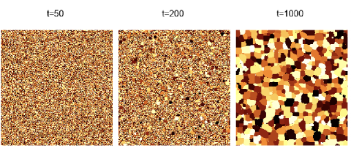
Figure 2: Snapshots at times $t=50,200,1000$ for a square lattice system with linear size $L=10^{3}$ and $q=10^{3}$. Different colors are different spin values.

Thus for a given value of $q$, after a quench at $T<T_{c}$, we observe metastable states up to a time which seems to diverge at some temperature value that we parametrise as $r_{t}(q)=T/T_{c}$. The quantity $r_{t}(q)$ does not seem to depend on the systems’ linear size considered. We found numerically $r_{t}(q=10^{3})\simeq 0.98$, $r_{t}(q=10^{4})\simeq 0.94$, $r_{t}(q=10^{5})\simeq 0.92$, $r_{t}(q=10^{6})\simeq 0.90$ and $r_{t}(q=10^{9})\simeq 0.87$. Thus, as we increase $q$, the temperature above which we observe metastable states forever slowly decreases. Presumably, this quantity will go to $0.5$ in the limit of infinite $q$.

For $T/T_{c}>r_{t}(q)$, we always observed metastable states. We will concentrate in the following in the study of these metastable states.

Figure 3: The time evolution of $N_{a}(t)/N$ for $a=3,6,10,11$ at $T=0.99\,T_{c}$ in a square lattice system with linear size $L=10^{3}$ and $q=10^{3}$. The thick lines are data from a numerical simulation while the thin ones are analytical predictions based on the method we develop in this work. The curves demonstrate the hierarchy in Eq. (29).

We illustrate the properties of these metastable states in Fig. 3, where we show the evolution of $N_{a}/N$ as a function of time for $q=10^{3}$ and $L=10^{3}$ at $T/T_{c}=0.99$. We only show the states which contribute the most. Already at times of the order of $t\simeq 10^{1}$ MCs after the quench, we found $N_{0}(t)=N_{2}(t)=N_{4}(t)=N_{7}(t)=N_{8}(t)=N_{9}(t)=0$ while $0\neq N_{1}(t)\simeq N_{5}(t)\simeq O(1)\ll N$ are not shown in the plot. The only values of order $N$ at this time scale are $N_{3}$, $N_{6}$, $N_{10}$ and $N_{11}$. Their expected values, according to the predictions based on the method we develop below, are $N_{11}/N\simeq 0.862,\,N_{6}/N\simeq 0.120,\,N_{3}/N\simeq 0.010,\,N_{10}/N\simeq 0.009$ and are shown with thin flat lines in the figure. The solid lines, instead, are the results of the numerical simulations, and are in excellent agreement with the analytic predictions. Statistically, the configurations do not change after running the simulation much longer: the state made of “vertices” (3), (6), (10) and (11) according to the hierarchy

$$N_{3}(t)\simeq N_{10}(t)\ll N_{6}(t)\ll N_{11}(t)$$ (29)

with all of them being ${\mathcal{O}}(N)$, is metastable over incredibly long time-scales.

In the following, we concentrate on cases in which $T$ is close to $T_{c}$. Moreover, we use the hierarchy relation (29) to develop an expansion that is notably accurate even keeping only the dominant order.

4.2 The leading updates at $T\simeq T_{c}$

We rename $N_{a}$ ($a=0,...,11$) the normalized (by $N$) abundances that can also be interpreted as the probabilities that a randomly picked site be in the state (a). Exploiting the hierarchy relation (29), expected to apply to the metastable state, we consider the evolution of

$$N_{11}\simeq 1\,,\qquad N_{6}\simeq p\,,\qquad N_{10}\simeq p^{2}\qquad\mbox{and}\qquad N_{3}\simeq p^{2}$$ (30)

thus rescaled with the parameter $p\equiv P_{11\rightarrow 6}$ which, at $T\simeq T_{c}$, is proportional to $q^{-1/2}$:

$$p\equiv P_{11\rightarrow 6}\simeq q^{-1/2}\qquad\mbox{for}\qquad T\sim T_{c}\;.$$ (31)

In the large $q$ limit, we will then use it as the small parameter in our expansion, that we will develop up to second order in powers of $p$.

Concretely, our aim now is to construct a master equation for the probabilities $N_{11}$, $N_{6}$, $N_{10}$, $\dots$, and then find the stationary solution that determines the proportions of the vertices of each kind in the metastable states.

In order to do so, we first picture what kind of structures, i.e., configurations of spins of the same color (spin value) in a background of “sand” (i.e. spins in the (11) state) have a probability to exist which is proportional to $p^{2}$ or greater. It turns out that spins in the states (6), (3) and (10), the only relevant ones in the large $N$ limit according to the discussion in the previous Subsection, can only be found in the following structures

where the gray sites in a given diagram possess the same color, while the white sites have a different color with respect to the gray ones and also with respect to the nearest and next-to-nearest other white ones. The numbers indicate the kind of vertex, following the notation used in the previous Subsections. The red segments, which highlight the satisfied bonds, are useful to keep track of the energy contribution of the structures. It is possible to check that all the other possible structures are of order $p^{3}$ or higher and we will not take them into account.

Now, we identify the evolutions that these structures can make in a single time step. As an example consider structure B. The following move

consists of a spin in state (11) turning into a state (6) and thus forming the structure on the right. The probability of this move is negligible because the probability to pick a (11) which is around the structure on the left (which contains (3)) is proportional to $p^{2}$ and the probability now for it to become a (6) is proportional to $p$. The result is therefore proportional to $p^{3}$ and hence negligible at the order we are keeping. This kind of analysis can be performed for all the cases and thus prove that the structures labelled A to F are at most of order $p^{2}$ and every other is negligible.

The next step is to list all the possible moves that are relevant for the second order of our expansion and understand what are the consequences of each of these moves. This will allow us to write down all the terms of the master equations for the probabilities $N_{11}$, $N_{6}$, $N_{3}$ and $N_{10}$. In practice we find that for (3) and (10) we need an equation for each of the configurations in which these states can be found so we define the following quantities

and

We can now express the probabilities for all the structures introduced above in terms of the probabilities of the various states

$$P(\textbf{A}) =(N_{6}-2N_{3a}-2N_{3b})/2\;,$$ (32)

$$P(\textbf{B}) =N_{3a}\;,$$

$$P(\textbf{C}) =N_{3b}=N_{10c}\;,$$

$$P(\textbf{D}) =N_{3c}/4\;,$$

$$P(\textbf{E}) =N_{10a}\;,$$

$$P(\textbf{F}) =N_{10b}/2\;,$$

where the first one comes from the fact that for every two (6) which are not in the structure B or C (which contain two (6) each) we count a structure A. The derivation of $P(\textbf{B}),\dots,P(\textbf{F})$ is straightforward. These expressions turn out to be useful to write down the probabilities of the moves, as we explain below.

Let us start with all the moves that a site which is in (11) can make. Pick a site in (11) which is not a neighbor of any structure and turn it into a (6). The probability for this move is

$$P_{11\rightarrow 6}=p,$$ (33)

where we mean the extended, temperature and $q$ dependent, form as in Eq. 26, times the probability of picking such a (11) state. The latter equals $N_{11}-3N_{6}$ because there are 3 sites in state $N_{11}$ surrounding every (6) in structure A, and we are neglecting the other terms of $P(\textbf{A})$ and the other structures because they will lead to contributions of higher orders. In this move we lose 2 (11) states and we gain 2 (6) states. In the following sketch we represent the move, we give its probability $P$ and we indicate below the sketch the loss and gain of vertices induced by the move.

$P=p(N_{11}-3N_{6})$

$-2N_{11},+2N_{6}$

In a similar way, the probability of all the other 15 possible moves (to order $p^{2}$) are computed in the Appendix.

4.3 The master equations

Collecting all the contributions for each of the probabilities $N_{a}$ we can now build the master equations governing their evolution in this approximation

$$\dot{N}_{11} =-N_{11}\frac{12}{4e^{\beta}+q-4}-2N_{11}p+2N_{6}-\frac{7}{4}N_{6}p-2N_{3a}+2N_{10b}+2N_{10a}$$ (34)

$$+2[(N_{3b}+N_{3a})P_{3\to 10}-(N_{10b}+N_{10a})P_{10\to 3}]$$ (35)

$$\dot{N}_{6} =2N_{11}p-2N_{6}+\frac{1}{2}N_{6}p+4(N_{3a}+N_{3b})+2(N_{3c}P_{3\to 10}-N_{10c}P_{10\to 3})$$ (36)

$$-2[(N_{3b}+N_{3a})P_{3\to 10}-(N_{10b}+N_{10a})P_{10\to 3}]$$ (37)

$$\dot{N}_{3a} =\frac{1}{4}N_{6}p-2N_{3a}-(N_{3a}P_{3\to 10}-N_{10a}P_{10\to 3})$$ (38)

$$\dot{N}_{3b} =\frac{1}{2}N_{6}p-2N_{3b}-(N_{3b}P_{3\to 10}-N_{10b}P_{10\to 3})+(N_{3c}P_{3\to 10}-N_{10c}P_{10\to 3})$$ (39)

$$\dot{N}_{3c} =-4(N_{3c}P_{3\to 10}-N_{10c}P_{10\to 3})$$ (40)

$$\dot{N}_{10a} =N_{11}\frac{4}{4e^{\beta}+q-4}-2N_{10a}+(N_{3a}P_{3\to 10}-N_{10a}P_{10\to 3})$$ (41)

$$\dot{N}_{10b} =N_{11}\frac{8}{4e^{\beta}+q-4}-2N_{10b}+2(N_{3b}P_{3\to 10}-N_{10b}P_{10\to 3})$$ (42)

$$\dot{N}_{10c} =\dot{N}_{3b}=\frac{1}{2}N_{6}p-2N_{3b}-(N_{3b}P_{3\to 10}-N_{10b}P_{10\to 3})+(N_{3c}P_{3\to 10}-N_{10c}P_{10\to 3}).$$ (43)

We want to solve the equations at stationarity, to do so we write down the probabilities in powers of $p$

$$N_{11} =\alpha_{0}+\alpha_{1}p+\alpha_{2}p^{2}$$ (44)

$$N_{6} =\beta_{1}p+\beta_{2}p^{2}$$

$$N_{3a} =\gamma_{2a}p^{2}$$

$$N_{3b} =\gamma_{2b}p^{2}$$

$$N_{3c} =\gamma_{2c}p^{2}$$

$$N_{10a} =\delta_{2a}p^{2}$$

$$N_{10b} =\delta_{2b}p^{2}$$

$$N_{10c} =\delta_{2c}p^{2}.$$

The normalization condition $N_{11}+N_{6}+N_{3a}+N_{3b}+N_{3c}+N_{10a}+N_{10c}+N_{10b}=1$ implies $\alpha_{0}=1$, $\beta_{1}=-\alpha_{1}$, $\alpha_{2}=-(\beta_{2}+\gamma_{2a}+\gamma_{2b}+\gamma_{2c}+\delta_{2a}+\delta_{2b}+\delta_{2c})$. Plugging the expressions in (44) in the master equation we find from $\dot{N}_{3c}=0$ that $\gamma_{2c}=\delta_{2c}P_{10\to 3}/P_{3\to 10}$, the first two equations contain first power terms of the form $2\alpha_{1}p+2p$, thus $\alpha_{1}=-1$ and by construction $\delta_{2c}=\gamma_{2b}$. We are left with

$$\dot{N}_{11} =-12xp^{2}+2p^{2}+2\beta_{2}p^{2}-\frac{7}{4}p^{2}-2\gamma_{2a}p^{2}+2\delta_{2b}p^{2}+\delta_{2a}p^{2}+$$ (45)

$$+2p^{2}[(\gamma_{2b}+\gamma_{2a})P_{3\to 10}-(\delta_{2b}+\delta_{2a})P_{10\to 3}]$$

$$\dot{N}_{6} =-2p^{2}-2\beta_{2}p^{2}+\frac{1}{2}p^{2}+4p^{2}(\gamma_{2a}+\gamma_{2b})$$

$$-2p^{2}[(\gamma_{2b}+\gamma_{2a})P_{3\to 10}-(\delta_{2b}+\delta_{2a})P_{10\to 3}]$$

$$\dot{N}_{3a} =\frac{1}{4}p^{2}-2\gamma_{2a}p^{2}-p^{2}(\gamma_{2a}P_{3\to 10}-\delta_{2a}P_{10\to 3})$$

$$\dot{N}_{3b} =\frac{1}{2}p^{2}-2\gamma_{2b}p^{2}-p^{2}(\gamma_{2b}P_{3\to 10}-\delta_{2b}P_{10\to 3})$$

$$\dot{N}_{10a} =4xp^{2}-2\delta_{2a}p^{2}+p^{2}(\gamma_{2a}P_{3\to 10}-\delta_{2a}P_{10\to 3})$$

$$\dot{N}_{10b} =8xp^{2}-2\delta_{2b}p^{2}+2p^{2}(\gamma_{2a}P_{3\to 10}-\delta_{2a}P_{10\to 3}),$$

where $x\equiv p^{-2}/(4e^{\beta}+q-4)$.
From $\dot{N}_{10a}=0$ we get

$$\delta_{2a}=\frac{4x+\gamma_{2a}P_{3\to 10}}{2+P_{10\to 3}},$$ (46)

from $\dot{N}_{3a}=0$

$$\gamma_{2a}=\frac{1/2+P_{10\to 3}/4+4xP_{10\to 3}}{4+2P_{10\to 3}+2P_{3\to 10}},$$ (47)

$\dot{N}_{10b}=0$ gives

$$\delta_{2b}=\frac{4x+\gamma_{2b}P_{3\to 10}}{1+P_{10\to 3}},$$ (48)

$\dot{N}_{10b}=0$

$$\gamma_{2b}=\frac{1/2+P_{10\to 3}/2+4xP_{10\to 3}}{2+2P_{10\to 3}+P_{3\to 10}},$$ (49)

and finally from $\dot{N}_{6}=0$

$$\beta_{2}=-3/4+2(\gamma{21}+\gamma{22})-[(\gamma_{2a}+\gamma_{2b})P_{3\to 10}-(\delta_{2b}+\delta_{2a})P_{10\to 3}].$$ (50)

Thus summarizing

$$\alpha_{0} =1$$ (51)

$$\alpha_{1} =-1$$

$$\alpha_{2} =-(\beta_{2}+\gamma_{2a}+\gamma_{2b}+\gamma_{2c}+\delta_{2a}+\delta_{2b}+\delta_{2c})$$

$$\beta_{1} =-\alpha_{1}$$

$$\beta_{2} =-3/4+2(\gamma{21}+\gamma{22})-[(\gamma_{2a}+\gamma_{2b})P_{3\to 10}-(\delta_{2b}+\delta_{2a})P_{10\to 3}]$$

$$\gamma_{2a} =\frac{1/2+P_{10\to 3}/4+4xP_{10\to 3}}{4+2P_{10\to 3}+2P_{3\to 10}}$$

$$\gamma_{2b} =\frac{1/2+P_{10\to 3}/2+4xP_{10\to 3}}{2+2P_{10\to 3}+P_{3\to 10}}$$

$$\gamma_{2c} =\delta_{2c}P_{10\to 3}/P_{3\to 10}$$

$$\delta_{2a} =\frac{4x+\gamma_{2a}P_{3\to 10}}{2+P_{10\to 3}}$$

$$\delta_{2b} =\frac{4x+\gamma_{2b}P_{3\to 10}}{1+P_{10\to 3}}$$

$$\delta_{2c} =\gamma_{2b}.$$

4.4 Numerical tests

In order to put the approach above to the numerical test, we collected the proportions $N_{a}$ measured with the heat bath Monte Carlo simulations and we compared them to the values computed with the master equation analysis. Concretely, we used systems with $L=10^{3}$, and $q=10^{4},\ 10^{5}$ and $10^{6}$, at $T/T_{c}=0.99$. The numerical and analytic data are displayed in Tab. 1. The number of digits shown correspond to results up to order $p^{2}$. The agreement between the values found with the two approaches is excellent.

$q$	10 000		100 000		1 000 000
	numerical	analytic	numerical	analytic	numerical	analytic
$N_{11}$	0.95731	0.95729	0.986509	0.986509	0.9957020	0.9957023
$N_{6}$	0.04054	0.04064	0.013269	0.013272	0.0042752	0.0042751
$N_{3a}$	0.00021	0.00021	0.000022	0.000022	0.0000023	0.0000023
$N_{3b}$	0.00042	0.00041	0.000044	0.000044	0.0000046	0.0000046
$N_{3c}$	0.00048	0.00046	0.000050	0.000050	0.0000053	0.0000053
$N_{10a}$	0.00019	0.00019	0.000020	0.000020	0.0000020	0.0000020
$N_{10b}$	0.00044	0.00041	0.000045	0.000044	0.0000046	0.0000046
$N_{10c}$	0.00037	0.00038	0.000039	0.000039	0.0000040	0.0000040

Table 1: $N_{a}$ for systems with $L=10^{3}$ and $q=10^{4},\ 10^{5},\ 10^{6}$ evolving at temperatures $T/T_{c}=0.99$ after an instantaneous quench from infinite temperature. The first column show the numerical values at MC times such that the system is stationary in the metastable state, while the second ones give the asymptotic values calculated with the master equations approach. Only the relevant values (up to order $p^{2}$) are shown. The error bars on the numerical values are always smaller than one on the last shown digits.

In Tab. 2 we show data for a system with linear size $L=10^{3}$ and $q=10^{6}$, and we vary the temperature, moving progressively towards criticality at $T_{c}$. As explained below, for this value of $q$, we observe a divergency of the time required to reach a ferromagnetic state at $T/T_{c}\simeq 0.9$. The data in Tab. 2 show that the analytic approximation is very good (in the metastable state) even moderately away from $T_{c}$. However, the numerical measurements at $T/T_{c}=0.88$ have been done at time $t=10^{3}$, and at this time the agreement between numerical and analytical data is still good but not as good as for the higher temperatures. In particular, one can notice a relatively important difference in $N_{11}$ and $N_{3c}$. For longer measuring times, one would see this difference increase, showing that the system leaves the metastable state at $T/T_{c}=0.88$. For the higher temperatures, there are no time-dependencies in the numerical results and for all purposes the metastable states remain for ever.

$T/T_{c}$	$p$		$\quad\quad N_{11}\quad\quad$	$\quad\quad N_{6}\quad\quad$	$\,10^{3}N_{3a}\,$	$\,10^{3}N_{3b}\,$	$\,10^{3}N_{3c}\,$	$\,10^{3}N_{10a}\,$	$\,10^{3}N_{10c}\,$
0.88	0.01017	numeric	0.9895816	0.0101646	0.0130	0.0260	0.1772	0.0020	0.0039
		analytic	0.9895916	0.0101674	0.0129	0.0259	0.1705	0.0020	0.0039
0.92	0.00725	numeric	0.9926679	0.0072481	0.0066	0.0132	0.0444	0.0020	0.0039
		analytic	0.9926690	0.0072485	0.0066	0.0131	0.0438	0.0020	0.0040
0.98	0.00459	numeric	0.9953845	0.0045892	0.0026	0.0053	0.0070	0.0020	0.0040
		analytic	0.9953847	0.0045892	0.0026	0.0053	0.0070	0.0020	0.0040
0.99	0.00428	numeric	0.9957020	0.0042752	0.0023	0.0046	0.0053	0.0020	0.0040
		analytic	0.9957023	0.0042751	0.0023	0.0046	0.0053	0.0020	0.0040

Table 2: $N_{a}$ for systems with linear size $L=10^{3}$, $q=10^{6}$ and various values of $T/T_{c}$ (corresponding to different values of $p$ ((second row)). For each temperature, the first line shows the numerical values at MC times such that the system is stationary in the metastable state, while the second ones give the asymptotic values calculated with the master equations approach. The error bars for the numerical values are of the order the last digit or smaller and they are not shown. We also have MC data for $N_{1}$, $10^{3}N_{1}=0.0044$ at $T/T_{c}=0.88$, $10^{3}N_{1}=0.0005$ at $T/T_{c}=0.92$, $10^{3}N_{1}=0.0000$ at $T/T_{c}=0.98$ and $T/T_{c}=0.99$.

Once the proportions $N_{a}$ are known it is possible to thermodynamically characterize the metastable states. For instance, we can evaluate the energy per spin of the disordered metastable state extended below the critical temperature, exploiting the stationary solutions obtained above. The only configurations that contribute to the energy are the $(6)$ ones with one bond and the $(3)$ ones with two bonds. Thus we have

$$e^{(d)}(\beta,q)=-\frac{1}{2}(N_{6}(\beta,q)+2N_{3}(\beta,q))\;,$$ (52)

where the $1/2$ factor avoids double counting of the bonds on the lattice. Note that for quench inverse temperature $\beta<\beta_{c}$ the expression in Eq. (52) should provide the equilibrium value of the energy at $\beta$. In Fig. 4 we plot the energy density of the disordered state as predicted by Eq. (52) as a function of $q$ at different ratios between the quench temperature and the critical one. The values of the energy density obtained with Monte Carlo simulations are also reported in the figure. The latter are time averages over single runs computed as long as the system stays in the metastable state (the error bars represent one standard deviation). A comparison with the exact mean field result for the energy at criticality [2] is reported. It is possible to appreciate that, for all temperatures, the energy decreases (in absolute value) approximatively as $q^{-1/2}$, this is expected because the major contribution to Eq. (52) is given by the $(6)$ term which scales indeed as $q^{-1/2}$ (see section above). Figure 5 shows instead the behaviour of the energy density of the disordered state as a function of the final quench temperature. The results of the expansion are again tested against Monte Carlo numerical simulations showing really good agreement.

Figure 4: Theoretical predictions in Eq. (52) and simulations results for the energy density of a system with $L=200$ when it is stuck in a paramagnetic metastable configuration, as a function of the number of states $q$, for several ratios of the quench temperature over the critical one. The numerical values are time averages over a single run. The error bars equal a standard deviation. The dashed tilted line correspond to the mean field exact result at criticality [2].

Figure 5: Energy density of the disordered metastable state vs $T/T_{c}$ for several values of $q$ (increasing from bottom to top), evaluated from Eq. (52) (colored solid lines). Values from simulations are also presented with data points. They are time averages of the energy density. The error bars correspond to a standard deviation. The critical temperature is indicated with a vertical black line.

5 Upper-critical quenches: the ordered metastable phase

As we anticipated above, the upper-critical protocol, which deals with the persistence of the ordered phase after a quench to a temperature $T>T_{c}$ starting from a fully ordered configuration, is less interesting from a technical point of view. We nonetheless perform a similar analysis (though less rich in terms of numerical evaluations) as for the disordered phase in order to complete the picture of metastability.

5.1 Large $q$ and large $N$ behaviour

Let us take the initial configuration to be at zero temperature, that is to say, a completely ordered state. Thus, the system is in one of the $q$ possible ground states and, consequently, all the $N$ sites are in state (0).

Recalling that (see Eq. (24)) for large $q$ we have $e^{\beta}\simeq q^{T_{c}/2T}$, during a lattice update, the probability for a state (0) to turn into a state (7) can be written as

$$P_{0\rightarrow 7}=\frac{q-1}{q+e^{4\beta}-1}\simeq\frac{q}{q+q^{2T_{c}/T}}=\frac{1}{1+q^{2T_{c}/T-1}}\ .$$ (53)

Thus, in the upper critical regime, the crossover temperature that separates two very different behaviours in the $q\rightarrow\infty$ limit is $T=2T_{c}$:

$$P_{0\rightarrow 7}\rightarrow 1\qquad\quad\mbox{at}\qquad\quad T>2T_{c}\;,$$ (54)

the (0) states turn into (7) states, and the system disorders really fast. At the crossover temperature

$$P_{0\rightarrow 7}\rightarrow 1/2\qquad\quad\mbox{at}\qquad\quad T=2T_{c}\;,$$ (55)

implying that states (7) can appear. Every (7) states will have as neighbours (1) states which (always in the limit $q\rightarrow\infty$) will become states (8) with probability $P_{1\rightarrow 8}\rightarrow 1$, and bring the system to a disordered configuration. Finally,

$$P_{0\rightarrow 7}\rightarrow 0\qquad\quad\mbox{at}\qquad\quad T<2T_{c}\;,$$ (56)

and the state (0) is completely stable in this temperature window close to $T_{c}$.

Going back to large but finite $q$, in Fig. 6, we show the evolution of $N_{a}$ as a function of time for $a=0,1$ and $7$, we only show the states which contribute the most.

Figure 6: $N_{a}(t)$ for $a=0,1,7$ evolving in time at $T=1.01\,T_{c}$ in a square lattice system with linear size $L=10^{3}$ and $q=10^{3}$. In thin lines are reported the analytical predictions obtained from the master equations below, in thick lines data from a numerical simulation. Note that the (1) and (7) abundances are one the vertical translation of the other. This is due to the fact that, by construction, there are four (1) states for every (7) one (see below).

Therefore, at upper critical temperatures, the following hierarchy holds

$$N_{1}\simeq N_{7}\ll N_{0}\simeq 1\ ,$$ (57)

where the $N_{a}$ are normalised by the number of spins in the sample, and all other states are negligible.

5.2 The leading updates at $T\simeq T_{c}$

Using again the expansion parameter $p$ with,

$$p^{2}\simeq q^{-1}\simeq P_{0\rightarrow 7}\qquad\quad\mbox{at}\qquad\quad T\sim T_{c}\;,$$ (58)

we consider the evolution of $N_{0}\simeq 1,N_{7}\simeq p^{2}$ and $N_{1}\simeq p^{2}$. Again we stop at second order in $p$.

It is straightforward to verify that the only structure that can appear in the sea of aligned spins (i.e., in the (0) state), with a probability proportional to $p^{2}$ or greater, is a (7) state surrounded by (1) states

Indeed there are only two ways to build different structures from the one above. The first one is that a (1), which has a probability proportional to $p^{2}$ to be picked, turns into a (4) or into an (8), respectively with probabilities $P_{1\rightarrow 4}\sim p^{2}$ and $P_{1\rightarrow 4}\sim p$. The other possibility is that a (0) close to a 1, which again has probability proportional to $p^{2}$ to be picked, turns into a (7), with probability $P_{0\rightarrow 7}\sim p^{2}$. The overall probabilities therefore are such that both scenarios are negligible in our approximation.

The only moves that should be taken into account to build a master equation for the ordered case are the switching of a (0) (surrounded by other (0) states) into a (7) and vice versa. In particular, we have that the probability of picking such a (0) is $N_{0}-8N_{7}$, because there are 8 (0) states next to a (1) surrounding each (7), but to the second order in $p$ we only retain $N_{0}$, and the probability for it to turn into a (7) creating in doing so also 4 (1) states is $P_{0\rightarrow 7}$

$P=N_{0}P_{0\rightarrow 7}$

$-5N_{0},+N_{7},+4N_{1}$

The inverse move, consistently, with probability $N_{7}P_{7\rightarrow 0}$ causes the destruction of 4 (1) states and of 1 (7) state creating 5 (0) states

$P=N_{7}P_{7\rightarrow 0}$

$-N_{7},-4N_{1},+5N_{0},$

5.3 The master equations

The master equations are therefore

$$\dot{N}_{0} =-5N_{0}P_{0\rightarrow 7}+5N_{7}P_{7\rightarrow 0}\$$ (59)

$$\dot{N}_{7} =-N_{7}P_{7\rightarrow 0}+N_{0}P_{0\rightarrow 7}\ \$$

$$\dot{N}_{1} =-4N_{7}P_{7\rightarrow 0}+4N_{0}P_{0\rightarrow 7}\ \ .$$

To solve them we write down the probabilities in powers of $p$

$$N_{0} =\alpha_{0}+\alpha_{1}p+\alpha_{2}p^{2}$$ (60)

$$N_{7} =\beta_{2}p^{2}$$

$$N_{1} =\gamma_{2}p^{2}.$$

By construction we have $N_{1}=4N_{7}$ and so $\gamma_{2}=4\beta_{2}$, moreover the normalization condition $N_{0}+N_{7}+N_{4}=1$ impose $\alpha_{0}=1$, $\alpha_{1}=0$ and $\alpha_{2}=-5\beta_{2}$. Finally, looking for the stationary solution of either one of the three differential equations above, we find $\beta_{2}=1/P_{7\rightarrow 0}$. Summarizing

$$\alpha_{0} =1\$$ (61)

$$\alpha_{1} =0\$$

$$\alpha_{2} =-5/P_{7\rightarrow 0}\$$

$$\beta_{2} =1/P_{7\rightarrow 0}\$$

$$\gamma_{2} =4/P_{7\rightarrow 0}\ .$$

5.4 Numerical tests

We can put the results from the previous section to the numerical test analysing, as for the disordered case, an interesting observable: the energy density of the metastable state. In this case the spin which falls in the $(0)$ configuration contributes with four bonds, while the ones in $(4)$ with three bonds. The ordered energy density thus reads

$$e^{(o)}(\beta,q)=-\frac{1}{2}(4N_{0}(\beta,q)+3N_{4}(\beta,q))\ .$$ (62)

This energy scales as $q^{-1}$ at fixed temperature, consistently with the fact that the major contribution comes from $(0)$. The agreement with the mean field results [2] and the outcome of the simulations analysed as in the disordered case is really good as can be checked by inspecting Fig. 7. The dependence of the energy density of the ordered state, as evaluated from Eq. (62), on temperature is portrayed in Fig. 8, where the comparison to the results of numerical evaluations shows again a perfect agreement.

Figure 7: Energy density of the ordered state as predicted by Eq. (62) and simulation data, for $L=200$, as a function of the number of states $q$, for several ratios of the quench temperature. The numerical values are averages in time of the energy for a single realisation, the error bars correspond to a standard deviation. Exact mean field predictions at criticality are reported as well (black dashed line) [2].

Figure 8: Ordered energy vs $T/T_{c}$ for several values of $q$, evaluated from Eq. (52). Values from simulations for $L=200$ are also present and are time averages for a single realization of the energy of the system as long as it stays in the metastable state, the error bars correspond to a standard deviation.

6 Conclusions

Most dynamic studies of the bidimensional Potts model focused on the analysis of the coarsening dynamics after deep quenches at moderate subcritical temperatures [6, 34, 35, 36] so as to avoid getting stuck in long-lived metastable configurations [37, 6, 38, 39, 40, 41]. The study of metastability and thermally assisted nucleation close to the critical temperature in this rather simple model has not been so much developed in the literature.

Numerical evidence for thermodynamic metastability in finite but large size systems with $q>4$ was provided in various papers. In particular, the analysis of the short-time dynamics [44] and Binder cumulant [45] was recently used with this purpose. However, Meunier and Morel [42] argued that thermodynamic metastability should disappear in the infinite system size limit and other authors [43] provided arguments supporting this claim. Extracting the infinite size limit behaviour, and the eventual disappearance of metastability from numerical studies is, however, a dauntingly hard task.

Last year, some of us wrote a short note on the nucleation and growth dynamics of the two dimensional Potts model [46]. With it we started our study of metastability in this (and eventually other) systems with first order thermal phase transitions. In this paper we developed a large $q$ expansion of the heat bath microscopic dynamics that allowed us to deduce, analytically, the metastability properties of the finite but large size model, in a rather wide range of temperatures around criticality (namely, from $T_{c}/2$ to $2T_{c}$). Although in the strictly infinite size limit the spinodals are expected to approach the critical point [42], we observe that the lifetime of the metastable state goes beyond reasonable times for relatively small system sizes. Our expansion allows us to capture the properties of these metastable states with amazing numerical accuracy.

Appendix A Appendix: Probability of the moves

Consider starting from a state (11) next to a structure A, turn it into a state (6), and make then a structure B be born. The probability of picking the starting site is $N_{6}$ because there are 2 (11) in such position for every structure A (again we are keeping only the terms which at the end will contribute up to the second order) and the probability to switch to (6) exactly in the needed direction is $p/4$. The probability of the move is thus $pN_{6}/4$ and we end up with with 1 (11) less and 1 (3a) more.

$P=pN_{6}/4$

$-N_{11},+N_{3a}$

The same move but with as a consequence a formation of a structure C has mutatis mutandis probability $pN_{6}/2$, and we lose 2 states (11) and gain 1 (3b) and 1 (10c):

$P=pN_{6}/2$

$-2N_{11},+N_{3b},+N_{10c}$

A site in a state (11) that is far from any structures and flips to another $q$ value but remains in the state (11) can, with probability $N_{11}4/(4e^{\beta}+q-4)$ assume the same colour of one of its next to nearest neighbours thus forming an E or, again with probability, $N_{11}4/(4e^{\beta}+q-4)$ form an F structure. We have, respectively,

$P=N_{11}(4/(4e^{\beta}+q-4))$

$-N_{11},+N_{10a}$

and

$P=N_{11}(4/(4e^{\beta}+q-4))$

$-2N_{11},+2N_{10b}$

Picking one of the two gray sites which are part of an E structure has probability $2P(\textbf{E})=2N_{10a}$. The probability for it to change colour but stay in a state (11) is $P_{11\rightarrow 11}=1-p$. Thus, the following move

$P=2N_{10a}$

$-N_{10a},+N_{11}$

occurs with probability $2N_{10a}$ and causes a loss of a (10a) and a gain of an (11)

Similarly, there are two gray (11) which are part of a structure F. Thus with probability $N_{10b}$ the following move cause a loss of 2 (10b) and the gain of 2 (11)

$P=N_{10b}$

$-2N_{10b},+2N_{11}$

Now we consider the cases when the starting state is a (6). The probability of picking a (6) which is part of a structure A is $2P(\textbf{A})=N_{6}-2N_{3a}-2N_{3b}$ and it turns to a (11) with probability $1-p$. So, to the second order in $p^{2}$, with probability $N_{6}(1-p)-2(N_{3a}+N_{3b})$, 2 (6) disappears and 2 (11) appears

$P=N_{6}(1-p)-2(N_{3a}+N_{3b})$

$-2N_{6},+2N_{11}$

Considering instead picking one of the two (6) which are part of a structure B or C, the transition to a (11) leads respectively with probability $2N_{3a}$ to a loss of 1 (3a) and a gain of a (11)

$P=2N_{3a}$

$-N_{3a},+N_{11}$

and with probability $2N_{3b}$ to the distruction of 1 (3b) and 1 (10c) and the creation of 2 (11)

$P=2N_{3b}$

$-N_{3b},-N_{10c},+2N_{11}$

Now we consider all the moves involving as starting sites a (3) or a (10) of all the possible kinds. This states, which can be picked with probability proportional to $p^{2}$ can turn one into the other with probabilities $P_{3\rightarrow 10}\sim 1/2$ and $P_{10\rightarrow 3}\sim 1/2$ for $T\simeq T_{c}$. Consider picking a (3a), this happens with probability $N_{3a}$, if it turns into a (10) (it happens with probability $P_{3\rightarrow 10}$) it cause the loss of 1 (3a) and 2 (6) and the gain of 1 (10a) and 2 (11)

$P=N_{3a}P_{3\rightarrow 10}$

$-N_{3a},-2N_{6},+N_{10a},+2N_{11}$

The inverse is

$P=N_{10a}P_{10\rightarrow 3}$

$-N_{10a},-2N_{11},+N_{3a},+2N_{6}$

If we pick a (3b), the probability of the move is $N_{3b}P_{3\rightarrow 10}$ and cause the destruction of 1 (3b), 1 (10c) and 2 (6) while creates 2 (10b) and 2 (11). We have

$P=N_{3b}P_{3\rightarrow 10}$

$-N_{3b},-N_{10c},-2N_{6},+2N_{10b},+2N_{11}$

and the opposite move with

$P=N_{10b}P_{10\rightarrow 3}$

$-2N_{10b},-2N_{11},+N_{3b},+N_{10c},+2N_{6}$

Finally, with probability $N_{3c}P_{3\rightarrow 10}$, 4 (3c) are destroyed and 1 (3b), 1 (10c) and 2 (6) are created by

$P=N_{3c}P_{3\rightarrow 10}$

$-4N_{3c},+N_{3b},+N_{10c},+2N_{6}$

the opposite of which happens with probability

$P=N_{10c}P_{10\rightarrow 3}$

$-N_{10c},-N_{3b},-2N_{6},+4N_{3c}$

References

- [1] R. B. Potts, Some generalised order-disorder transformations, Proc. Cambridge Phil. Soc. 48, 106 (1952).
- [2] F. Y. Wu, The Potts model, Rev. Mod. Phys. 54, 235 (1982).
- [3] R. J. Baxter, Exactly solved models in statistical mechanics, 1st edition (Academic Press, 1982).
- [4] D. Weaire and N. Rivier, Soap, cells and statistics - random patterns in two dimensions, Contemp. Phys. 25, 59 (1984).
- [5] J. Stavans, The theory of cellular structures, Rep. Prog. Phys. 56, 733 (1993).
- [6] J. Glazier, M. Anderson and G. S. Grest, Coarsening in the 2-dimensional soap froth and the large Potts model - a detailed comparison, Phil. Mag. B 62, 615 (1990).
- [7] A. D. Sokal, Chromatic polynomials, Potts models and all that, Physica A 279, 324 (2000).
- [8] J. Salas and A. D. Sokal, Transfer matrices and partition-function zeros for antiferromagnetic Potts models. I. General theory and square-lattice chromatic polynomial, J. Stat. Phys. 104, 609 (2001).
- [9] M Blatt, S. Wiseman, and E. Domany, Superparamagnetic Clustering of Data, Phys. Rev. Lett. 76, 3251 (1996).
- [10] J. Reichardt and S. Bornhold, Detecting fuzzy community structures in complex networks with a Potts model, Phys. Rev. Lett. 93, 218701 (2004).
- [11] P. Ronhovde, D. Hu, and Z. Nussinov, Global disorder transition in the community structure of large-q Potts systems, EPL 99, 38006 (2012).
- [12] Vik. S. Dotsenko, Vl. S. Dotsenko, M. Picco, and P. Pujol, Renormalization group solution for the two-dimensional random bond Potts model with broken replica symmetry, Europhys. Lett. 32, 425 (1995).
- [13] Vl. S. Dotsenko, M. Picco, and P. Pujol, Renormalisation group calculation of correlation functions for the 2D random bond Ising and Potts models, Nucl. Phys. B 455, 701 (1995).
- [14] T. R. Kirkpatrick and D. Thirumalai, Mean-field soft-spin Potts glass model - statics and dynamics, Phys. Rev. B 37, 5342 (1988).
- [15] D. Thirumalai and T. R. Kirkpatrick, Mean-field Potts glass model - initial-condition effects on dynamics and properties of metastable states, Phys. Rev. B 38, 4881 (1988).
- [16] T. R. Kirkpatrick, D. Thirumalai and P. G. Wolynes, Scaling concepts of the dynamics of viscous liquids near an ideal glassy state, Phys. Rev. A 40, 1045 (1989).
- [17] G. Biroli and L. Berthier, Theoretical perspective on the glass transition and amorphous materials, Rev. Mod. Phys. 83, 587 (2011).
- [18] T. R. Kirkpatrick and D. Thirumalai, Colloquium: Random first order transition theory concepts in biology and physics, Rev. Mod. Phys. 87, 183 (2015).
- [19] J. D. Gunton, M. San Miguel and P. S. Sahni, in Phase Transitions and Critical Phenomena vol 8, eds. C Domb and J L Lebowitz (New York: Academic, 1983).
- [20] K. Binder, Theory of first order phase transitions, Rep. Prog. Phys. 50, 783 (1987).
- [21] D. W. Oxtoby, Homogenoeus nucleation: theory and experiment, J. Phys.: Condens. Matter 4, 7627 (1992).
- [22] K. F. Kelton and A. L. Greer, Nucleation in Condensed Matter (Elsevier, Amsterdam, 2010).
- [23] R. J. Baxter, Potts model at the critical temperature, J. Phys. C 6, L445 (1973).
- [24] L. Mittag and M. J. Stephen, Mean-field theory of the many component Potts model, J. Phys. A: Gen. Phys. 7, L109 (1974).
- [25] A. Baracca, M. Bellesi, R. Livi, R. Rechtman, and S. Ruffo, On the mean field solution of the Potts model, Phys. Lett. A 99, 156 (1983).
- [26] K. Binder, Static and dynamic critical phenomena of the two-dimensional -state Potts model, J. Stat. Phys. 24, 69 (1981).
- [27] K. Nam, B. Kim and S. J. Lee, Nonequilibrium critical relaxation of the order parameter and energy in the two-dimensional ferromagnetic Potts model, Pays. Rev. E 77, 056104 (2008).
- [28] X. Huang, S. Gong, F. Zhong and S. Fan, Finite-time scaling via linear driving: Application to the two-dimensional Potts model, Phys. Rev. E. 81, 041139 (2010).
- [29] C. D. Li, D. R. Tan and F. J. Jiang, Applications of neural networks to the studies of phase transitions of two-dimensional Potts models, Annals of Physics 391, 312 (2018).
- [30] S. Iino, S. Morita, N. Kawashima, and A. W. Sandvik, Detecting Signals of Weakly First-order Phase Transitions in Two-dimensional Potts Models, J. Phys. Soc. Japan 88, 034006 (2019).
- [31] F. Y. Wu, The infinite-state potts model and restricted multidimensional partitions of an integer, Mathematical and Computer Modelling 26, 269 (1997).
- [32] J. Johansson and M. E. Pistol, Microcanonical entropy of the infinite-state Potts model, Physics Research International, 2011, ID 437093 (2011).
- [33] R. Burioni, F. Corberi, and A. Vezzani, Complex phase-ordering of the one-dimensional Heisenberg model with conserved order parameter, Phys. Rev. E 79, 041119 (2009).
- [34] A. Petri, M. Ibáñez de Berganza and V. Loreto, Ordering dynamics in the presence of multiple phases, Phil. Mag. 88, 3931 (2008).
- [35] M. P. O. Loureiro, J. J. Arenzon, and L. F. Cugliandolo, Curvature-driven coarsening in the two-dimensional Potts model, Phys. Rev. E 81, 021129 (2010).
- [36] M. P. O. Loureiro, J. J. Arenzon, and L. F. Cugliandolo, Geometrical properties of the Potts model during the coarsening regime, Phys. Rev. E 85, 021135 (2012).
- [37] I. M. Lifshitz, Kinetics of Ordering During Second-Order Phase Transitions, JETP 42, 1354 (1962).
- [38] E. E. Ferrero and S. A. Cannas, Long-term ordering kinetics of the two-dimensional q-state Potts model, Phys. Rev. E 76, 031108 (2007).
- [39] M. Ibáñez de Berganza, E. E. Ferrero, S. A. Cannas, V. Loreto, and A. Petri, Phase separation of the Potts model in the square lattice, Eur. Phys. J. Special Topics 143, 273 (2007).
- [40] J. Olejarz, P. Krapivsky and S. Redner, Zero-temperature coarsening in the 2d Potts model, J. Stat. Mech. P06018 (2013).
- [41] J. Denholm and S. Redner, Topology-controlled Potts coarsening, Phys. Rev. E 99, 062142 (2019).
- [42] J. L. Meunier and A. Morel, Condensation and Metastability in the 2D Potts Model, Eur. Phys. J. B 13, 341 (2000).
- [43] M. Ibáñez Berganza, P. Coletti, A. Petri, Anomalous metastability in a temperature-driven transition, EPL 106, 56001 (2014).
- [44] E. S. Loscar, E. E. Ferrero, T. S. Grigera and S. A. Cannas, Nonequilibrium characterization of spinodal points using short time dynamics, J. Chem. Phys. 131, 024120 (2009).
- [45] E. E. Ferrero, J. P. De Francesco, N. Wolovick and S. A. Cannas, q-state Potts model metastability study using optimized GPU-based Monte Carlo algorithms, Comp. Phys. Comm. 183, 1578 (2011).
- [46] F. Corberi, L. F. Cugliandolo, M. Esposito, and M. Picco, Multinucleation in the first-order phase transition of the 2d Potts model, J. Phys. Conf. Series 1226, 012009 (2019).