OGLE-2018-BLG-0677Lb: A SUPER EARTH NEAR THE GALACTIC BULGE

Abstract

We report the analysis of the microlensing event OGLE-2018-BLG-0677. A small feature in the light curve of the event leads to the discovery that the lens is a star-planet system. Although there are two degenerate solutions that could not be distinguished for this event, both lead to a similar planet-host mass ratio. We perform a Bayesian analysis based on a Galactic model to obtain the properties of the system and find that the planet corresponds to a super-Earth/sub-Neptune with a mass $M_{\mathrm{planet}}={3.96}^{+5.88}_{-2.66}\mathrm{M_{\oplus}}$. The host star has a mass $M_{\mathrm{host}}={0.12}^{+0.14}_{-0.08}\mathrm{M_{\odot}}$. The projected separation for the inner and outer solutions are ${0.63}^{+0.20}_{-0.17}$ AU and ${0.72}^{+0.23}_{-0.19}$ AU respectively. At $\Delta\chi^{2}=\chi^{2}({\rm 1L1S})-\chi^{2}({\rm 2L1S})=46$, this is by far the lowest $\Delta\chi^{2}$ for any securely-detected microlensing planet to date, a feature that is closely connected to the fact that it is detected primarily via a “dip” rather than a “bump”.

1 INTRODUCTION

In the study of astronomical bodies, the search for extra-solar planets is of particular interest as their characterization not only allows us to infer the similarities or differences in the mechanisms of their formation, but it also helps us to better understand our own solar system (Ollivier et al., 2008). There is a wide range of methods for planet discovery such as radial velocity (RV), transit photometry, microlensing, direct imagining, etc. This has been a huge leap since the first confirmed discovery of an extra-solar planet more than 20 years ago (Cochran et al., 1991); to date there are four thousand extra-solar planets ($\simeq$ 4104 as of December 2019), with the majority ($\geq 3000$) having been found by the transit method.

Gravitational microlensing is a particular type of gravitational lensing for which both source and lens are stellar mass objects and the angular size of the magnified images cannot be resolved (Vietri & Ostriker, 1983; Paczyński, 1986; Schneider et al., 2006; Tsapras, 2018, etc). Instead, we study the difference in brightness of the source produced by the gravitational interaction of the lens when it crosses through the line of sight (Einstein, 1936; Paczyński, 1986; Schneider et al., 2013; Mollerach & Roulet, 2002; Mao, 2012, etc). Although, it was theorized since the formulation of gravitational lensing, the very small likelihood of the necessary alignment discouraged its observation as having low probability. The proposition had a resurgence in interest following the work of Paczyński (1986), which led to the start of microlensing observations with the first detection in 1993 (Alcock et al., 1993; Udalski et al., 1993).

Mao & Paczyński (1991) pointed out how the formalism for binary lenses and the feasibility of their observation could be used for detecting either binary systems or a planetary system. This was developed by several authors in the following years (Gould & Loeb, 1992; Griest & Hu, 1992; Gould, 2000; Albrow et al., 2000; Bennett et al., 2002; An et al., 2002; Ratttenbury, 2006, etc). Nevertheless, it took almost a decade for the first confirmed exoplanet by a microlensing observation to be published by Bond et al. (2004).

Currently there are over 80 confirmed planets discoveries through microlensing observations. The rate of detections has increased in recent years with the advent of the Korean Microlensing Telescope Network (KMTNet) (Kim et al., 2016).

This work addresses the microlensing event OGLE-2018-BLG-0677. This is a relatively-faint, moderate-magnification event with some evidence for an anomaly soon after peak brightness. From a comparison with single-lens, binary-lens and binary-source models, we will show a strong preference for a binary lens interpretation. As we can only obtain directly two physical quantities for the system we perform a Bayesian analysis to infer the probable physical properties for the host (lens) and companion. The resulting distributions suggest that the companion is a low-mass planet.

In Section 2 of this paper we briefly describe the observations of the event. Section 3 describes our model selection, as well as the details of the light curve fitting process, and presents the best-fit values. In Section 4, we investigate the angular size of the source and its implications for the Einstein radius, and in Section 5 we give a detailed description of the approach taken for the Bayesian analysis used to infer the properties of the lensing system, and present the resulting distributions. From these we derive the planet mass and the separation from its host. In Section 6 we discuss some of the implications of this work and, finally, Section 7 is a brief discussion concluding the paper.

2 OBSERVATIONS

2.1 OGLE

The event was first detected by the Optical Gravitational Lensing Experiment (OGLE) Early Warning System (EWS, Udalski et al. 1994; Udalski 2003), with designations OGLE-2018-BLG-0677 and OGLE-2018-BLG-0680, since it lies in the overlap region of two survey fields. It is located at $(RA,Dec)=(17^{h}55^{m}00^{s}.27,-32^{\circ}00^{\prime}59".51)$ , which corresponds to $(l,b)=(-1^{\circ}.61,-3^{\circ}.31)$ in Galactic coordinates. In combination, the observations from the two fields have a frequency of 1-3 data points per day. The OGLE observations were reduced using difference image analysis (DIA) from Wozniak (2000).

2.2 KMTNet

The Korea Microlensing Telescope Network (KMTNet) is a wide-field imaging system, with three telescopes and cameras sharing the same specifications, installed at Cerro-Tololo Inter-American Observatory in Chile (KMTC), the South African Astronomical Observatory in South Africa (KMTS), and the Siding Spring Observatory in Australia (KMTA). The telescopes each have a 1.6 m primary mirror, and a wide-field camera (a mosaic of four $9k\times 9k$ CCDs) that image approximately a $2.0\times 2.0$ square degree field of view.

Weather permitting, the network of telescopes and cameras allow a 24 hour per day monitoring of the Galactic Bulge. This allows one to trace the light curves of stars continuously and is ideal for the detection of extrasolar planets by microlensing and transit, variable objects, and asteroids and comets.

The event OGLE-2018-BLG-0677 was independently detected by KMTNet and given the designation KMT-2018-BLG-0816 (Kim et al., 2018). The event is located in the BLG01 and BLG41 KMTNet fields, giving an effective observation cadence of 15 minutes.

Photometry was extracted from the KMTNet observations using the software package PYDIA (MichaelDAlbrow, 2017), which employs a difference-imaging algorithm based on the modified- delta-basis-function approach of Bramich et al. (2013). The light curve of the event, with a single lens single source (1L1S) model, is shown in Fig. 1.

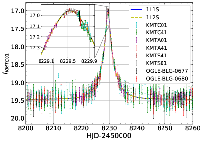
Figure 1: Light curve for OGLE-2018-BLG-0677 fitted with 1L1S and 1L2S models (which overlap and cannot be distinguished visually). The small window zoomed into the section of the light curve presents a small anomaly, which cannot be accounted for by the models.

3 LIGHT CURVE ANALYSIS

The following sections present the several models fitted to the data as well as the reasoning by which we selected the best among them.

3.1 Single lens single source

This is the simplest of models, which considers a point mass lens with a point mass source. The magnification is modeled by a Paczyński (1986) curve,

$$A(u)=\frac{u^{2}+2}{u\sqrt{u^{2}+4}},$$ (1)

where $u$ is the angular separation between source and lens normalized by the Einstein angle $\theta_{\rm E}$. Given the relative motion between them, this separation will be a function of time and is assumed rectilinear as

$$u(t)=(\tau^{2}+u^{2}_{0})^{1/2}\,,$$ (2)

with $\tau\equiv(t-t_{0})/t_{\rm E}$; $u_{0}$ is the impact parameter of the event, $t_{0}$ is the time at $u=u_{0}$, and $t_{\rm E}$ is the Einstein radius crossing time. These three parameters characterize completely the light-curve magnification model, $A(t)$. We find these parameters by a Markov Chain Monte Carlo (MCMC) search while reducing the $\chi^{2}$ of a linear fit to the observed flux, $F(t)=A(t)F_{\rm S}+F_{\rm B}$, where the source and blend flux, $F_{\rm S}$ and $F_{\rm B}$, are determined for each data set.

The best-fit values (after renormalization of data uncertainties as will be discussed in Section 3.4) are presented in Table 1. We note that in Tables 1-3, $F_{\text{S}}$ and $F_{\text{B}}$ are given in a system with 18 as the magnitude zero point.

Table 1: Best-Fit 1L1S Model parameters.

$\chi^{2}_{min}/N_{\text{data}}$	$1602.51/1557$
$u_{0}$	$0.1029\pm 0.0012$
$t_{0}$	$8229.5417\pm 0.0007$
$t_{\rm E}$ (days)	$4.95\pm 0.04$
$F_{\text{S,OGLE0677}}$	$0.293\pm 0.009$
$F_{\text{B,OGLE0677}}$	$-0.065\pm 0.011$

3.2 Anomaly

As can be seen in Figure 1, there is a small anomalous feature in the light curve relative to the 1L1S model that occurs over $\sim$ 5 hr during the interval 8229.70 - 8229.90. The anomaly primarily takes the form of a dip of $\sim 0.05$ mag followed by a smaller and shorter bump. See the residuals in Figure 2. These features are well traced by the KMTC01 and KMTC41 data sets, and they are confirmed by two points from the OGLE-2018-BLG-0680 data, one each on the dip and the subsequent small bump. The OGLE-2018-BLG-0677 data set has a single point just before the start of the anomaly. We have examined the direct and difference images from KMTC and are satisfied that there are no systematic effects that can be attributed to seeing, background, or image cosmetics that could cause these features. Additionally, we have found no evidence that the dip is a repeating phenomenon, such as might be due to a star spot.

3.3 Single lens binary source

We examine the possibility that the anomaly is due to a binary source. In the case that the source consists of two stars, the total flux is given by the linear combination of the individual source fluxes, $F_{\rm tot}=A_{1}F_{1}+A_{2}F_{2}+F_{\rm B}$, where $A_{1}$ and $A_{2}$ are the individual magnifications of each source (Gaudi, 1998) as parameterized in Section 3.1, but sharing the same value of $t_{\rm E}$.

The total magnification of the combined source flux is given by

$$A_{\rm tot}=\frac{A_{1}+A_{2}q_{F}}{1+q_{F}}\,,$$ (3)

where $q_{F}=F_{2}/F_{1}$ is the luminosity ratio (Griest & Hu, 1992). In total, there are 6 parameters: $u_{01}$ and $t_{01}$ for $A_{1}$, $u_{02}$ and $t_{02}$ for $A_{2}$, $t_{\rm E}$ is shared by $A_{1}$ and $A_{2}$;  and the luminosity ratio $q_{F}$. We fit the data as described in the previous subsection but using this model instead. The best-fit values found for the data are presented in Table 2, and the light-curve model shown in Figure 2. It is apparent that the best binary source model does not reproduce the anomalous feature in the light curve, but produces a small “bump” deviating almost imperceptibly from the 1L1S model.

Table 2: Best-Fit 1L2S Model parameters

$\chi^{2}_{min}/N_{\text{data}}$	$1593.08/1557$
$u_{01}$	$0.103\pm 0.004$
$t_{01}$	$8229.542\pm 0.004$
$u_{02}$	${0.05}^{+0.31}_{-0.05}$
$t_{02}$	${8229.873}^{+0.546}_{-0.061}$
$q_{F}$	${0.0031}^{+0.0317}_{-0.0028}$
$t_{\rm E}$ (days)	$4.96\pm 0.14$
$F_{\text{S,OGLE0677}}$	$0.287\pm 0.009$
$F_{\text{B,OGLE0677}}$	$-0.063\pm 0.011$

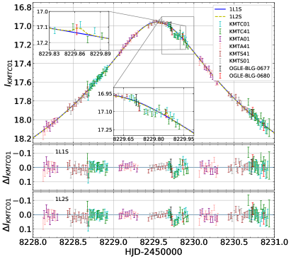
Figure 2: Light curve for OGLE-2018-BLG-0677, together with 1L1S (solid line) and 1L2S (dashed line) (upper panel) and residuals from these models (lower two panels). It is clear the two solutions overlap and predict essentially the same light curve, except for an interval of 0.5 hours near 8229.86

3.4 Binary lens

We adopt the standard parameterization of a binary lens light curve by describing it with 7 parameters (Gaudi, 2012): $s$, $q$, $\rho_{\ast}$, $\alpha$, $u_{0}$, $t_{0}$ and $t_{\rm E}$. These represent the normalized separation between binary-lens components, the mass ratio of the binary-lens components, the normalized source radius, the source-trajectory angle with respect to the binary axis, the normalized closest approach between the lens center of mass and the source (which occurs at time $t_{0}$, the time of closest approach), and the timescale to cross the Einstein radius, respectively. The factor used for the normalized parameters is the angular Einstein radius,

$$\theta_{\rm E}=\sqrt{\frac{4GM_{L}}{c^{2}}\left(\frac{1}{D_{L}}-\frac{1}{D_{S}}\right)},$$ (4)

where $M_{L}$ is the total mass of the lens system, and $D_{L}$, $D_{S}$ are the distances from Earth to the lens and source. A visualization of this combination of parameters can be found in Jung et al. (2015).

The fitting is done by a Maximum Likelihood Estimation, which is equivalent to minimization of the $\chi^{2}$. The process is done in two parts. The first is through a fixed value grid search of the $(s,q)$ parameters to find regions where the minimum $\chi^{2}$ may be located. For each $(s,q)$, a grid of $(r,\alpha)$ (where $r$ is a reparameterization of $u_{0}$, centred-on and normalized to caustics, see McDougall & Albrow (2016)) is used to seed a minimization over ($\rho_{\ast},t_{0},t_{\rm E})$ by a simple Nelder-Mead optimization (Nelder & Mead, 1965). This approach for the fixed $(s,q,r,\alpha)$ is due to the relation of these parameters to the geometry.

Our fixed position results are then used as seeds for a more refined search using a Markov Chain Monte Carlo (MCMC) algorithm implemented by using the MORSE code (McDougall & Albrow, 2016). A similar two step process can also be seen in Shin et al. (2019). During this second part of the process, the seed solutions from the grid search are used as starting points, and the search is now continuous in the parameter space.

Once a minimum value for $\chi^{2}$ was found, the original magnitude uncertainties for each data set were renormalized via

$$\sigma^{\prime}_{i}=k\sqrt{\sigma_{i}^{2}+\epsilon^{2}}.$$ (5)

The coefficients $k$ and $\epsilon$ for each data set are determined in such a way that the reduced $\chi^{2}$ for both the higher- and lower-magnification data points for each site are approximately unity (Yee et al., 2012). The renormalization factors are listed in Table 6. The MCMC search was then re-run with the renormalized data uncertainties to corroborate the solution and obtain a new minimized $\chi^{2}$. The final model parameter values and their uncertainties are directly obtained from the 68% confidence interval around the medians of the marginalized posterior parameter distributions.

Given the short total time of the event, it was not possible to obtain parallax information (Gould, 1992; Alcock et al., 1995; Gould, 2000; Buchalter & Kamionkowski, 2002). For the rest of our analysis, no higher order light-curve effects were considered.

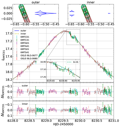
Figure 3: Best-fit models for binary lens and corresponding caustic geometries. The upper panels show the two possible geometries of inner and outer solution. The remaining panels show the observed light curve for both solutions, which are indistinguishable, and their respective residuals.

3.4.1 Model of OGLE-2018-BLG-0677

From the fitting process described in the previous section, we found two degenerate solutions with similar $q$. Often this situation corresponds to a well-known wide/close case degeneracy where $s<1$ and $s>1$ for the two solutions  (see e.g., Griest & Safizadeh, 1998; Dominik, 1999; Batista et al., 2011). However, in the present case, the degeneracy is between two solutions with $s<1$, and is due to a source-trajectory passage past two cusps of connected or disconnected caustics, as shown in Figure 3. Each corresponds to a minor-image perturbation, that demagnifies the source relative to the magnification due solely to the host star. This type of degeneracy has been detected previously for events OGLE-2012-BLG-0950 (Koshimoto et al., 2017) and OGLE-2016-BLG-1067 (Calchi Novati et al., 2019). A thorough explanation of the phenomenon is given in Han et al. (2018) with reference to the event MOA-2016-BLG-319. Following the nomenclature of that paper, we refer to the case where the source passes between the caustics as the ”inner” solution, and that where it passes the single connected caustic as the ”outer” solution.

For the current event, OGLE-2018-BLG-0677, we could not break this degeneracy given that both cases produce almost identical light curves, see Figure 3. Table 3 lists the best-fit parameters for both solutions. Apart from the clear difference in geometry, they share several parameters, $q$, $u_{0}$, $t_{0}$, $t_{\rm E}$, well within their respective uncertainties. Also, the values of the minimum $\chi^{2}$ are close enough that there is no clear statistical difference. Despite this degeneracy, the similarities of $q$, $\rho$ and $t_{\rm E}$ will allow us to infer similar physical properties for the system, which will be discussed in the following section.

As a note, $\rho_{\ast}$ is detected rather weakly in the light-curve analysis. It may be of interest to ask whether the omission of $\rho_{\ast}$ affects our subsequent results in any significant way.

Therefore in section 5.2 we give results that propagate the $\rho_{\ast}$ distribution, and also show the the case where the $\rho_{\ast}$ information is omitted from the Bayesian estimates.

Table 3: Best-Fit Binary Model parameters

	inner	outer
$\chi^{2}_{min}/N_{\text{data}}$	$1556.03/1557$	$1555.96/1557$
$s$	${0.912}^{+0.002}_{-0.054}$	${0.985}^{+0.059}_{-0.002}$
$\log_{10}q$	${-4.105}^{+0.305}_{-0.0822}$	${-4.054}^{+0.268}_{-0.109}$
$\rho_{\ast}$	${0.01209}^{+0.00013}_{-0.00545}$	${0.01238}^{+0.00016}_{-0.00590}$
$u_{0}$	$0.102\pm 0.003$	$0.102\pm 0.003$
$\alpha$	$-1.98\pm 0.01$	$4.307\pm 0.008$
$t_{0}$	$8229.544\pm 0.002$	$8229.544\pm 0.002$
$t_{\rm E}$ (days)	$4.94\pm 0.11$	$4.94\pm 0.11$
$F_{\text{S,OGLE0677}}$	$0.294\pm 0.009$	$0.294\pm 0.009$
$F_{\text{B,OGLE0677}}$	$-0.069\pm 0.011$	$-0.070\pm 0.011$

3.4.2 Other local minima

Five additional seed solutions were identified in our initial grid search close, located close in $(s,q)$ to the solutions reported above. All of these are very shallow in $\chi^{2}$-space, and with subsequent MCMC runs, all converged to one of either of the reported solutions. Light curves and caustic geometries for the two most prominent of these local minima are shown in Figure 4.

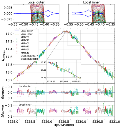
Figure 4: Light-curve fit and geometries for the local inner and outer minimum models for binary lens. These two solutions are degenerate with each other, but disfavored relative to the best-fit models shown in Figure 3.

Table 4: Local Minima Binary Model parameters

	inner	outer
$\chi^{2}_{min}/N_{\text{data}}$	$1580.19/1557$	$1579.82/1557$
$s$	$1.030$	$1.082$
$\log_{10}q$	$-3.732$	${-3.725}$
$\rho_{\ast}$	$0.031$	$0.031$
$u_{0}$	$0.107$	$0.107$
$\alpha$	$1.498$	$1.498$
$t_{0}$	$8229.543$	$8229.543$
$t_{\rm E}$ (days)	$4.837$	$4.852$
$F_{\text{S,OGLE0677}}$	$0.279\pm 0.001$	$0.276\pm 0.001$
$F_{\text{B,OGLE0677}}$	$-0.020\pm 0.002$	$-0.018\pm 0.002$

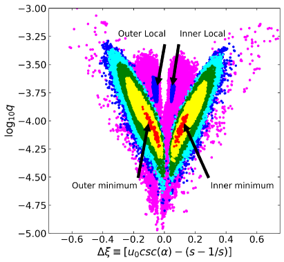
Figure 5: Scatter plot of $\Delta\xi$ vs. $\log_{10}q$, where $\Delta\xi$ is the offset between the center of the source and the caustic as the source crosses the planet-star axis. Color coding is red, yellow, green, cyan, blue, magenta for $\Delta\chi^{2}<1,4,9,16,25,36$. Values of $\Delta\chi^{2}>36$ are omitted given the closeness to the 1L1S model, $\Delta\chi^{2}\sim 10$, and also to help the readability of the scatter plot.

To analyze how these local minima are related to the best-fit solutions, we followed the procedure described in Hwang et al. (2017) and ran various “hot” and “cold” MCMC realisations to explore the regions around all the solutions. In Figure 5 we present a scatter plot of the combined samples from the various runs, color coded by their $\Delta\chi^{2}$ relative to the best solutions. We adopt the parameter

$$\Delta\xi=u_{0}\csc\alpha-(s-1)/s,$$ (6)

introduced by Hwang et al. (2017), which traces the offset between the centers of the source and the major-image caustic as the source crosses the planet - star axis. Three of the identified extra solutions are located within the purple region below the best-fit solutions, with $25<\Delta\chi^{2}<36$, and are indistinguishable from their surroundings. The two remaining local minima, i.e. those displayed in Figure 4 and labelled as outer and inner local minima in Figure 5, have $16<\Delta\chi^{2}<25$. They are degenerate, and correspond to a lens mass ratios $~{}\sim$ twice that of the best solutions. They each represent a source trajectory over an on-axis cusp that provides a single bump in magnification, and correspond to a major-image perturbation with degeneracies as discussed in Gaudi & Gould (1997).

Their light curve fit parameters are listed in Table 4, without uncertainties as they are too shallow in $\chi^{2}$ space to retain an MCMC chain. They have a similar $t_{E}$ to the best solutions, but a larger $\rho_{*}$.

3.5 Model selection

From Figure 1, it can be seen that there is a subtle anomaly following the peak of the light curve compared to the 1L1S model. Although a binary lens model could in principle represent this small feature found in the data, the justification for the increase in model complexity needs to be strengthened; therefore, to avoid overfitting by assuming a binary lens (Gaudi, 1997), we compared with two simpler models. The three models compared are the previously-described single lens single source (1L1S), single lens binary source (1L2S) and binary lens single source (2L1S) models. Often the $\chi^{2}$ value is used as an indicator of the goodness-of-fit, but this time instead of simply relying on this statistic to compare between different models, we obtain the log evidence given the data, $\ln\mathcal{Z}$, for a more robust model comparison. This was done by applying the Nested Sampling method (Skilling, 2006) for cases (1L1S) and (1L2S). For the case of (2L1S), nested-sampling was too inefficient, so the approximation algorithm presented in van Haasteren (2009) for posterior distributions was used instead to estimate $\ln\mathcal{Z}$. For completeness, we also applied the approximate algorithm to the other two cases, which led to the same results as nested sampling. The log odds ratio is obtained by $\ln O=\ln\mathcal{Z}_{M1}-\ln\mathcal{Z}_{M2}$, and a model is preferred as long as $\ln O>0$, but a strong preference is given when $\ln O>5$ (Sivia & Skilling, 2006; Jaynes et al., 2003).

The 2L1S best-fit has two degenerate solutions, inner and outer (see Griest & Safizadeh, 1998), but the difference in $\chi^{2}$ between these ($\Delta\chi^{2}=0.07$) is small, with a slight preference to the outer model. On the other hand, the log evidence gives a strong preference for the inner model. We need to adopt a model for renormalization, so we decided to choose the inner solution for this purpose.

Table 5 shows the the minimum $\chi^{2}$ and the log evidence based on the renormalized data error bars, and it is clear that the 2L1S solution is preferred with $\Delta\chi^{2}>46$ compared with the 1L1S, and is also preferred from the evidence.

One last consideration worth mentioning is the case for 1L2S. From the $\chi^{2}$ point of view it seems to improve compared to 1L1S, however the evidence gives an indication that the 1L1S is slightly better. Here the meaning of the evidence becomes clear. It says that the 1L2S model is not better than the 1L1S, (the extra model complexity does not outweigh the reduction in $\chi^{2}$), and it in fact the difference with the 1L1S model is only between 8229.85 and 8229.88. This can be clearly seen in Figure 2 with the 1L1S and 1L2S “best-fit” light curves.

Table 5: Minimum $\chi^{2}$ and log evidence for 1557 data points for the different lensing models.

Model	1L1S	1L2S	2L1S(inner)	2L1S(outer)
$\chi^{2}_{\rm renorm}$	1602.51	1593.08	1556.03	1555.96
$\ln\mathcal{Z}_{\rm renorm}$	-811.33	-815.11	-806.15	-807.23
$\Delta\chi^{2}_{\rm renorm}$	0.00	9.43	46.48	46.55
$\Delta\ln\mathcal{Z}_{\rm renorm}$	0.0	-4.29	5.18	4.1

4 COLOR MAGNITUDE DIAGRAM

A sample instrumental color magnitude diagram (CMD) for a 1.5 x 1.5 arcmin field around OGLE-2018-BLG-0677 is shown in Figure 6 based on KMTC data. The source position is indicated, with its magnitude determined from the source flux inferred by the light-curve model, and its color from a regression of $V$-band difference flux against $I$-band difference flux.

From an analysis of four such CMDs (KMTC01, KMTC41, KMTS01, and KMTS41), we found a color offset from the red clump, $(V-I)_{s}-(V-I)_{\rm RC}=-0.47\pm 0.04$, and a magnitude offset, $I_{s}-I_{\rm RC}=3.20\pm 0.03$. Combining these with the red clump intrinsic color, $(V-I)_{\rm RC,0}=1.06$ (Bensby et al., 2013) and magnitude for this Galactic longitude, $I_{\rm RC,0}=14.534$ (Nataf et al., 2013), we find for the source that $(V-I)_{0,s}=0.59\pm 0.04$ and $I_{0,s}=17.73\pm 0.03$.

From Bessell & Brett (1988) we convert our color to $(V-K)_{0}=1.25\pm 0.10$, and using the surface-brightness relations of Kervella et al. (2004) we determine the source angular radius $\theta_{\ast}=0.789\pm 0.025$ $\mu$as.

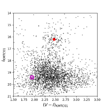
Figure 6: Color magnitude diagram of the field from the KMTC01 images. The red clump centroid is shown as a red dot, and the source, inferred from the light-curve model fit, is shown as (very small) magenta error bars, with a magenta circle to highlight its position.

Table 6: Renormalization values.

inner/outer	scale factor	added uncertainty
KMTC01	2.543	0.003
KMTC41	3.038	0.006
KMTA01	1.904	0.006
KMTA41	3.04	0.000
KMTS01	1.956	0.005
KMTS41	1.828	0.003
OGLE-BLG-0677	1.429	0.031
OGLE-BLG-0680	1.463	0.020

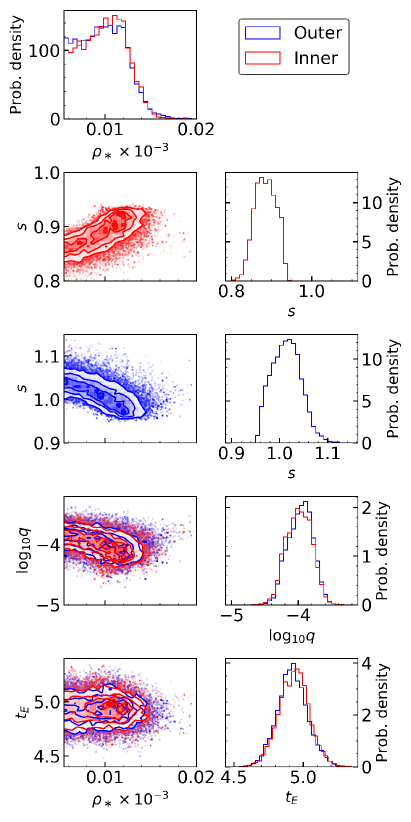
Figure 7: MCMC chains and posterior distributions. The first left panel displays the fully-marginalized distributions for $\rho_{\ast}$, which shows how the inner and outer distributions overlap. The right panels show the fully-marginalized distributions for $s$, $log_{10}q$ and $t_{E}$ for the outer (blue) and inner (red) solutions, which will be used to derive the properties of the host and companion. The four left lower panels show the Markov chain points for these parameters projected against $\rho_{\ast}$.

5 PROPERTIES OF THE LENSING SYSTEM

In the previous sections we presented the results from the light-curve fitting, from which our sources of physical information are $t_{\rm E}$ and $\rho_{\ast}$. Also, we could not break the outer/inner geometry, but fortunately the fitting showed that the majority of the parameters are similar within their uncertainties (see Table 3), in particular the crossing time $t_{\rm E}$. Doing a direct comparison of the posterior distributions for both solutions, it is clear that they also share a similar distribution of $\rho_{\ast}$ as seen in Figure 7, despite the $s$ distributions being different. This becomes important because we can proceed to the Galactic model expecting a priori that both solutions will share similar characteristics.

5.1 Bayesian Analysis

We performed a Bayesian analysis to characterize the physical properties of the system. As remarked above, our source of information from the light curve comes only from the distributions of $t_{\rm E}$ and $\rho_{\ast}$, which restricts how much information we can gather. In other words, we need to limit the number of parameters used in the analysis to the most basic. The main parameters are the total mass of the lens, $M_{L}$, the distance to the lens, $D_{L}$, the proper motion, $\mu_{rel}$, and the source distance, $D_{S}$. Nevertheless, during the formulation of the analysis, the effective transverse velocity $v=D_{L}\mu_{rel}$ will be used as an intermediate step during the parameter sampling.

Our analysis resembles a hierarchical Bayes (see e.g., Gelman et al., 2003),

$$p(\Theta|y)\propto p(\Theta)\int{p(t_{\rm E},\rho_{\ast}|\Theta)p(y|t_{\rm E},\rho_{\ast})}dt_{\rm E}d\rho_{\ast}\,,$$ (7)

where

$${\Theta} \equiv (M_{L},D_{L},D_{S},v)$$ (8)

$$y \equiv \text{data}\,.$$ (9)

This describe the probability distribution function for $t_{\rm E}$ and the weights based on the distribution of $\rho_{\ast}$, which is shown in Figure 7. The prior sampling distribution for the physical quantities is $p(\Theta)$ , which includes the information of the Galactic model. For the analysis, $t_{\rm E}$ and $\rho_{\ast}$ act as constraints, and they are hidden in $p(t_{\rm E},\rho_{\ast}|\Theta)$, which is the probability of a value of $t_{\rm E}$ and $\rho_{\ast}$ given by the physical parameters.

For this purpose we took a combined approach in which we perform an MCMC simulation to obtain the posterior distribution from the Galactic modelling. Ideally, we would describe the process in observable variables similar to Batista et al. (2011); Yee et al. (2012) or Jung et al. (2018), but in this case we are only able to relate two observables to the physical parameters, $t_{\rm E}$ and $\rho_{\ast}$. We therefore take advantage of the Monte Carlo simulation to take care of the marginalization. We used two different sampling algorithms in order to verify that our results contain no algorithmic bias. Independently, we ran the Emcee sampler (Foreman-Mackey et al., 2013) which uses the standard Metropolis-Hasting sampling method, and Dynesty (Higson et al., 2018) which uses Nested Sampling. After convergence, both algorithms arrived at the same posterior distributions.

Our approach is similar to that of Yoo et al. (2004), but we describe our Galactic model and the fact that we can define the probability of a physical property given an observed parameter, e.g., $p(\Theta|t_{\rm E}^{(0)})$, as presented in Dominik (1998); Albrow et al. (2000).

For the Galactic model, the lens mass function, $\Phi_{\log m}$, is a power law or Gaussian distribution depending on the mass ranges according to Chabrier (2003). The mass density distribution, $\Phi_{x}(x)$, considers the disk, bulge or both depending on the case, where the disk is modelled by a double exponential with $0.3$ kpc and $1.0$ kpc as the scale heights of a thin and thick disk perpendicular to the Galactic plane, and the corresponding column mass densities are $\Sigma_{\text{thin}}=25\,\text{M}_{\odot}\text{pc}^{-2}$ and $\Sigma_{\text{thick}}=35\,\text{M}_{\odot}\text{pc}^{-2}$. For the bulge we adopt a model of a barred bulge that is tilted by an angle of $20^{\circ}$ (see Grenacher et al., 1999; Han & Gould, 1995). The probability density of the absolute effective velocity, $\Phi_{\nu}(\nu,x)$, assumes Gaussian distributions, for which isotropic velocity dispersions are assumed for the Galactic disk and bulge, and the values of $\sigma^{\text{{disk}}}=30\,\text{km}\text{s}^{-1}$ and $\sigma^{\text{bulge}}=100\,\text{km}\text{s}^{-1}$are adopted. While the velocity mean for Bulge objects is assumed purely random, the disk lenses rotation velocity can described by a NFW model (see Navarro et al., 1997). The precise equations for each component of the Galactic model can be found in the appendices of Dominik (2006).

Therefore, the probability of our assumed Galactic model (galactic prior) for the lens is in the form

$$p_{i}(m,\zeta,x)\propto\Phi_{\log m}(\log m)\Phi_{\zeta}(\zeta,x)\Phi_{x}(x)\,,$$ (10)

selecting from bulge or disk populations accordingly. The parameters in this prescription are the mass $m=M_{L}/\text{M}_{\odot}$, the fractional lens-source distance, $x=D_{L}/D_{S}$, and the effective transverse velocity $\zeta=v/v_{c}$, where $v_{c}=100\,\text{km}\,\text{s}^{-1}$ is a scaling constant to keep the velocity dimensionless. These distributions and prescriptions can also be found in Dominik (2006), and, as mentioned above, the assumed properties are described in its appendix.

The source distance probability distribution is defined as

$$p_{source}(D_{S})=\frac{D_{S}^{\gamma}\rho(D_{S})}{\int^{D_{s,max}}_{0}{D_{S}^{\gamma}\rho(D_{S})}dD_{S}},$$ (11)

where $\rho(D_{S})$ is the density of objects at the source distance as defined in Dominik (2006). We adopted this distribution as we do not have any information on the source location, and we based its definition on the Zhu et al. (2017) argument, but we use a value of $\gamma=1$. For our calculations, we assumed that the source was part of the bulge population.

Therefore, the Galactic prior, which has the Galactic model information, is sampled from the probability distribution

$$p(\Theta)\propto\Omega(m,\zeta,x)p_{i}(m,\zeta,x)p_{source}(D_{S}).$$ (12)

The lens for bulge or disk populations are selected accordingly. Meanwhile, the information of the prior is weighted by

$$\Omega(m,\zeta,x)\propto(M/M_{\odot})^{1/2}\zeta\sqrt{x(1-x)}.$$ (13)

(Dominik, 2006). The parameter $t_{\rm E}$ then becomes intrinsic and is defined as

$$t_{\rm E}(m,\zeta,x,D_{S}) = \frac{2r_{E,\odot}\sqrt{mx(1-x)}}{\zeta{v_{c}}}\,,$$ (14)

where

$$r_{E,\odot} = \sqrt{\frac{G\text{M}_{\odot}}{c^{2}}D_{S}}$$ (15)

is a scale length defined as the Einstein radius of a solar mass lens located half-way between the observer and source.

The angular source size parameter,

$$\rho_{\ast}(m,x,D_{S})=\theta_{\ast}/\theta_{\rm E}(m,x,D_{S})\,,$$ (16)

where $\theta_{\ast}$ is the source angular radius given in the previous section and $\theta_{\rm E}(m,x,D_{S})$ is the Einstein angle for a MCMC realization.

Given that $\rho_{\ast}$ and $t_{\rm E}$ are derived from the prior parameters, their joint probability

$$p(t_{\rm E},\rho_{\ast}|\Theta)\propto\delta(t_{\rm E}-t_{\rm E}(\Theta))\delta(\rho_{\ast}-\rho_{\ast}(\Theta))\,.$$ (17)

Additionally, there is a weight given by the information contained in the probability distribution $p(y|t_{\rm E},\rho_{\ast})$, which corresponds to the posterior distributions of our solution from our light-curve fitting.

The simplest to represent is the value of $t_{\rm E}$, as it is well constrained and reduces simply to

$$p(y|t_{\rm E})\propto\exp\left(-\frac{(t_{\rm E}-t_{E,{best}})^{2}}{2\sigma_{t_{\rm E}}^{2}}\right)\,.$$ (18)

Here $t_{E,{\rm best}}$ and $\sigma_{t_{\rm E}}$ correspond to the values from the best fit of the distribution from the light-curve fitting.

For the case of $\rho_{\ast}$, it is not as simple because the constraint is not well approximated as a Gaussian. We introduce the information by the use of $\Delta\chi^{2}=\chi^{2}-\chi^{2}_{min}$ of each of the light-curve fitting samples. From the lower envelope of these samples, binned in $\rho_{\ast}$, we obtain a numerical function $\Delta\chi^{2}(\rho_{\ast})$, see Figure 8. The probability of $\rho_{\ast}$ is then given by

$$p(y|\rho_{\ast})\propto\exp\left(-\frac{\Delta\chi^{2}(\rho_{\ast})}{2}\right)\,.$$ (19)

The previous weights are combined as

$$p(y|t_{\rm E},\rho_{\ast})\propto p(y|\rho_{\ast})p(y|t_{\rm E})\,.$$ (20)

The information of the Galactic model is introduced into Equation (20) by the restriction imposed by the Dirac $\delta$ function in Equation (17).

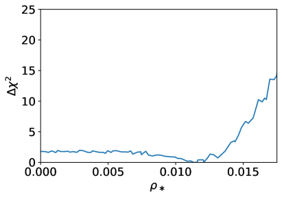
Figure 8: Minimum $\Delta\chi^{2}$ as a function of $\rho_{\ast}$ using the chains derived from the light-curve fitting MCMC. This shows that $\rho_{\ast}$ is weakly detected as there is clearly an upper limit for it, but the difference from a flat region on the smaller values is only $\Delta\chi^{2}\approx 1.7$.

The combination of the prior and these weights gives the desired posterior probability for the physical parameters, where $\mu_{rel}$ is appropriately obtained from $\zeta$. We note that both outer and inner models lead to the same final results. This is expected given the similarity of the $t_{\rm E}$ and $\rho_{\ast}$ distributions.

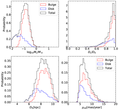
Figure 9: Posterior probability distributions from the Bayesian analysis for the lens mass $log_{10}M_{L}/M_{\odot}$, the ratio of the lens and source distance $D_{L}/D_{S}$, the source distance $D_{S}$ and $\mu_{rel}$. In addition to the total, the four panels show also the separate bulge and disk distributions, normalized to the total.

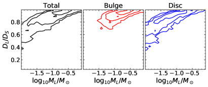
Figure 10: 1, 2, and 3-sigma contour levels for the distributions of the lens mass $log_{10}M_{L}/M_{\odot}$ and the ratio of the lens and source distance $D_{L}/D_{S}$ . In addition to the total, the panel show also the separate bulge and disk distributions.

Table 7: Estimators from the Bayesian results

$\log_{10}{M_{L}/M_{\odot}}$	$D_{L}/D_{S}$	$D_{S}$[kpc]	$\mu_{rel}$[mas/year]
${-0.94}^{+0.34}_{-0.47}$	${0.92}^{+0.05}_{-0.12}$	${8.37}^{+1.06}_{-1.07}$	${7.02}^{+2.48}_{-1.68}$

5.2 Resulting properties

The distributions obtained from the Galactic modelling are presented in Figure 9, and the corresponding estimators for the median and error values are in Table 7. As noted above, the outer and inner solutions produce indistinguishable distributions.

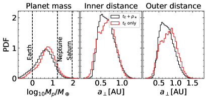
Figure 11: Derived distributions for the planet mass and projected separation, $a_{\perp}$[AU], in Astronomical Units for outer and inner solutions. The red line shows the change caused by removing information about $\rho_{\ast}$ from the Galactic model evaluation.

From the resulting distributions of the basic four parameters, the lens mass, lens distance, source distance and proper motion, we can propagate the information to derive the physical mass of the binary lens components and their physical separation. Additionally, the host-mass distribution is essentially identical to the total lens-mass distribution in Figure 9. In this case, the binary-lens mass ratio is small, and the host consists of a low mass star or brown dwarf with a super-Earth companion. As mentioned previously, given the overlapping of the distributions of $t_{\rm E}$ and $q$ for the inner and outer solutions, the Bayesian analysis returns indistinguishable distributions, and for these reasons it is justifiable to say that both give the same derived planet mass distribution. This is not the case for the projected separation between host and planet, which has a small but not negligible difference. The derived distributions are shown in Figure 11 and their estimators in Table 8.

Furthermore, as mentioned at the end of 3.4.1, the value for $\rho_{\ast}$ is weakly constrained. The relatively broad and highly non-Gaussian form of this constraint is shown in Figure 8. For comparison purposes, in Figure  11, we show alongside the complete Galactic modeling, which includes the information of $t_{\rm E}$ and $\rho_{\ast}$, the derived distributions produced by removing the information about $\rho_{\ast}$ and using only $t_{\rm E}$. In such a case, the planet mass distribution is shifted a little higher, and the projected separation distributions are a little broader. Their estimators are also included in Table 8.

Table 8: Estimators for the planet mass and projected separation

	$\log_{10}{M_{p}/M_{\oplus}}$	$a_{\perp}$(Inner)	$a_{\perp}$(Outer)
$t_{\rm E}+\rho_{\ast}$	${0.60}^{+0.40}_{-0.48}$	${0.63}^{+0.20}_{-0.17}$ AU	${0.72}^{+0.23}_{-0.19}$ AU
$t_{\rm E}$ only	${0.73}^{+0.37}_{-0.45}$	${0.64}^{+0.19}_{-0.21}$ AU	${0.80}^{+0.23}_{-0.26}$ AU

The inner and outer solutions for the planet in OGLE-2018-BLG-0667 both imply that the secondary lens is a super-Earth/Sub-Neptune planet with a mass $M_{\mathrm{planet}}={3.96}^{+5.88}_{-2.66}\mathrm{M_{\oplus}}$, while the host is a dwarf star or brown-dwarf with mass $M_{\mathrm{host}}={0.12}^{+0.14}_{-0.08}M_{\sun}$.

The projected separation between the star and planet is ${0.63}^{+0.20}_{-0.17}$ AU and ${0.72}^{+0.23}_{-0.19}$ AU for the inner and outer solutions, respectively. The lens system is estimated to be at a distance of ${7.58}^{+1.15}_{-1.35}$ kpc, with a 66.9% probability of lying in the bulge (Figure 9).

For completeness, we note the physical implications of the solutions corresponding to the two local minima discussed in Section 3.4.2. Since these are degenerate with each other in $q$, $t_{\rm E}$ and $\rho_{*}$, they imply the same primary and secondary lens mass and distance. The local minima would imply a total lens mass of 0.1 $M_{\odot}$ and a planet mass of 6.43 $M_{\oplus}$, values very similar to the favoured solutions, but a lens located at a distance of 0.99 $D_{S}$. The projected separation of the planet from its host would be smaller, either 0.20 or 0.22 AU, for the inner and outer local minima respectively.

6 DISCUSSION

OGLE-2018-BLG-0677Lb has the lowest $\Delta\chi^{2}$ relative to the best 1L1S model of any planet securely detected by microlensing. One of the first microlensing planets, OGLE-2005-BLG-0390 (Beaulieu et al., 2006) also had one of the lowest improvements relative to 1L1S, $\Delta\chi^{2}=960$. One reason such seemingly high formal thresholds are generally required for secure microlensing planet detections is that “bumps”, particularly those without clear caustic features, can in principle be produced by 1L2S models (Gaudi, 1998; Jung et al., 2017; Shin et al., 2019).

In the case, of OGLE-2005-BLG-390, the 1L2S model was ruled out by just $\Delta\chi^{2}=46$. Moreover, Udalski et al. (2018) examined whether OGLE-2005-BLG-390 would have been detectable if the planet-host mass ratio were lower. They concluded that at factors $q^{\prime}/q<0.63$ it would not have been because the resulting $\Delta\chi^{2}=\chi^{2}({\rm 1L2S})-\chi^{2}({\rm 2L1S})\leq 13$ would have been too marginal to claim reliable detection of a planet. Note that this threshold for unambiguous identification corresponds to $\Delta\chi^{2}=\chi^{2}({\rm 1L1S})-\chi^{2}({\rm 2L1S})\simeq 457$, which is almost ten times the value for OGLE-2018-BLG-0677.

However, OGLE-2018-BLG-0677 is detected primarily through a dip in the light curve, which cannot be reproduced by any 1L2S scenario, or any other higher-order microlensing effect. The only other possible cause for the observed dip is a systematic error in the photometry. This is extremely unlikely because the signal is detected in the data from two overlapping KMTC fields that were reduced independently, and is confirmed by two data points from the OGLE telescope, located at a different observatory, and with images reduced by different software.

With a relative lens-source proper motion greater than 5 mas/yr, the separation between lens and source will be sufficient for them to be separately resolved within a decade with the advent of IR adaptive optics imaging on either present-day or under-construction extremely large telescopes. We have no detection of flux from the blend in the current event, and so we expect that the lens is at least ten times fainter than the source, $I_{\rm lens}>22$. This implies that to be confident that a non-detection of the lens implies a non-luminous (i.e., brown-dwarf) lens, these observations should be carried out after the lens and source have separated by at least 1.5 FWHM, i.e., $12\,{\rm yr}(\lambda/1.6\,\mu{\rm m})/(D/10\,{\rm m})$ after $t_{0}$ (i.e., 2018). Here $\lambda$ is the wavelength of the observations and $D$ is the diameter of the mirror.

7 SUMMARY

We have presented an analysis of the microlensing event OGLE-2018-BLG-0677/OGLE-2018-BLG-0680/KMT-2018-BLG-0816.

The light curve of the event exhibits a small dip, soon after peak on an otherwise-smooth Paczyński-like magnification profile. The dip lasts for $\sim 3.5$ hours and is followed by a smaller bump lasting $\sim 1.5$ hours. These features are well traced by the KMTNet CTIO observations from two telescope pointings and are confirmed by the OGLE-2018-BLG-0680 light curve.

We have fitted several models to the light curve and obtained their $\chi^{2}$ and evidence. The light curves for 1L2S and 1L1S models are virtually identical and do not reproduce the anomalous feature in the observations.

We also presented the fit for binary lens solutions. These suffer from a two-fold inner-outer(close-wide) degeneracy, but we found that the ratio of masses was similar for both, indicating that the lens is composed of a star plus planet system. Formally, the planet is detected with a $\Delta\chi^{2}\approx 46$ and $\Delta\ln\mathcal{Z}=5$ relative to the single lens models.

Using the binary solutions we performed a Bayesian analysis and found that outer and inner solutions agree with the same distribution for the lens mass, lens distance and proper motion.

The derived planet mass is $M_{\mathrm{planet}}={3.96}^{+5.88}_{-2.66}\mathrm{M_{\oplus}}$, one of the lowest yet detected by microlensing. In Figure 12 we use data from the NASA Exoplanet Archive to show the mass and separation of confirmed exoplanets found with different methods such as microlensing, radial velocity or transits. (An example of how the mass is derived for the latter can be found in Espinoza et al. 2016.)

It can be seen that the planet mass and distance reported in this work are consistent with the lower limit of masses that have been found previously through microlensing, and also consistent with their separation range. This event reinforces the importance of high-cadence microlensing observations, which allow us to detect and characterize anomalies due to low-mass planets.

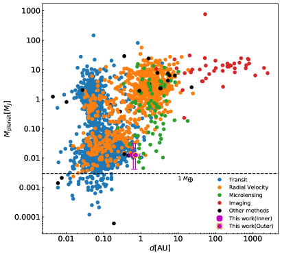
Figure 12: Masses and orbital radii of confirmed exoplanets detected via different methods. A dashed line indicates where Earth-mass planets would lie. The data for the confirmed exoplanets can be found in NASA Exoplanet Archive (https://exoplanetarchive.ipac.caltech.edu).

References

- Albrow et al. (2000) Albrow, M. D., Beaulieu, J.-P., Caldwell, J. A. R., et al. 2000, The Astrophysical Journal, 534, 894, doi: 10.1086/308798
- Alcock et al. (1993) Alcock, C., Akerlof, C. W., Allsman, R. A., et al. 1993, Nature, 365, 621, doi: 10.1038/365621a0
- Alcock et al. (1995) Alcock, C., Allsman, R. A., Alves, D., et al. 1995, The Astrophysical Journal, 454, doi: 10.1086/309783
- An et al. (2002) An, J. H., Albrow, M. D., Beaulieu, J., et al. 2002, The Astrophysical Journal, 572, 521, doi: 10.1086/340191
- Batista et al. (2011) Batista, V., Gould, A., Dieters, S., et al. 2011, Astronomy & Astrophysics, 529, A102, doi: 10.1051/0004-6361/201016111
- Beaulieu et al. (2006) Beaulieu, J. P., Bennett, D. P., Fouqué, P., et al. 2006, Nature, 439, 437, doi: 10.1038/nature04441
- Bennett et al. (2002) Bennett, D. P., Becker, A. C., Quinn, J. L., et al. 2002, The Astrophysical Journal, 579, 639, doi: 10.1086/342225
- Bensby et al. (2013) Bensby, T., Yee, J. C., Feltzing, S., et al. 2013, A&A, 549, A147, doi: 10.1051/0004-6361/201220678
- Bessell & Brett (1988) Bessell, M. S., & Brett, J. M. 1988, PASP, 100, 1134, doi: 10.1086/132281
- Bond et al. (2004) Bond, I. A., Udalski, A., Jaroszyski, M., et al. 2004, The Astrophysical Journal, 606, L155, doi: 10.1086/420928
- Bramich et al. (2013) Bramich, D. M., Horne, K., Albrow, M. D., et al. 2013, Monthly Notices of the Royal Astronomical Society, 428, 2275, doi: 10.1093/mnras/sts184
- Buchalter & Kamionkowski (2002) Buchalter, A., & Kamionkowski, M. 2002, The Astrophysical Journal, 482, 782, doi: 10.1086/304163
- Calchi Novati et al. (2019) Calchi Novati, S., Suzuki, D., Udalski, A., et al. 2019, AJ, 157, 121, doi: 10.3847/1538-3881/ab0106
- Chabrier (2003) Chabrier, G. 2003, Publications of the Astronomical Society of the Pacific, 115, 763, doi: 10.1086/376392
- Cochran et al. (1991) Cochran, W. D., Hatzes, A. P., & Hancock, T. J. 1991, The Astrophysical Journal, 380, L35, doi: 10.1086/186167
- Dominik (1998) Dominik, M. 1998, Astronomy and Astrophysics, 330, 963
- Dominik (1999) —. 1999, Astronomy & Astrophysics, 125, 108
- Dominik (2006) —. 2006, Monthly Notices of the Royal Astronomical Society, 367, 669, doi: 10.1111/j.1365-2966.2006.10004.x
- Einstein (1936) Einstein, A. 1936, Science, 84, 506, doi: 10.1126/science.84.2188.506
- Espinoza et al. (2016) Espinoza, N., Brahm, R., Jordán, A., et al. 2016, The Astrophysical Journal, 830, 43, doi: 10.3847/0004-637X/830/1/43
- Foreman-Mackey et al. (2013) Foreman-Mackey, D., Hogg, D. W., Lang, D., & Goodman, J. 2013, Publications of the Astronomical Society of the Pacific, 125, 306, doi: 10.1086/670067
- Gaudi (1997) Gaudi, B. S. 1997, The Astrophysical Journal, 489, 508, doi: 10.1086/304791
- Gaudi (1998) —. 1998, The Astrophysical Journal, 506, 533, doi: 10.1086/306256
- Gaudi (2012) —. 2012, Annual Review of Astronomy and Astrophysics, 50, 411, doi: 10.1146/annurev-astro-081811-125518
- Gaudi & Gould (1997) Gaudi, B. S., & Gould, A. 1997, ApJ, 486, 85, doi: 10.1086/304491
- Gelman et al. (2003) Gelman, A., Carlin, J. B., Stern, H. S., & Rubin, D. B. 2003, Bayesian Data Analysis, Second Edition, Chapman & Hall/CRC Texts in Statistical Science (Taylor & Francis). https://books.google.co.nz/books?id=TNYhnkXQSjAC
- Gould (1992) Gould, A. 1992, The Astrophysical Journal, 392, 442, doi: 10.1086/171443
- Gould (2000) —. 2000, The Astrophysical Journal, Volume 542, Issue 2, pp. 785-788., 542, 785, doi: 10.1086/317037
- Gould & Loeb (1992) Gould, A., & Loeb, A. 1992, ApJ, 396, 104, doi: 10.1086/171700
- Grenacher et al. (1999) Grenacher, L., Jetzer, P., Strässle, M., & de Paolis, F. 1999, A&A, 351, 775. https://arxiv.org/abs/astro-ph/9909374
- Griest & Hu (1992) Griest, K., & Hu, W. 1992, The Astrophysical Journal, 397, 362, doi: 10.1086/171793
- Griest & Safizadeh (1998) Griest, K., & Safizadeh, N. 1998, The Astrophysical Journal, 500, 37, doi: 10.1086/305729
- Han & Gould (1995) Han, C., & Gould, A. 1995, The Astrophysical Journal, 447, 53, doi: 10.1086/175856
- Han et al. (2018) Han, C., Bond, I. A., Gould, A., et al. 2018, The Astronomical Journal, 156, 226, doi: 10.3847/1538-3881/aae38e
- Higson et al. (2018) Higson, E., Handley, W., Hobson, M., & Lasenby, A. 2018, Statistics and Computing, doi: 10.1007/s11222-018-9844-0
- Hwang et al. (2017) Hwang, K.-H., Udalski, A., Shvartzvald, Y., et al. 2017, The Astronomical Journal, 155, 20, doi: 10.3847/1538-3881/aa992f
- Jaynes et al. (2003) Jaynes, E. T., Jaynes, E. T. J., Bretthorst, G. L., & Press, C. U. 2003, Probability Theory: The Logic of Science (Cambridge University Press). https://books.google.co.nz/books?id=tTN4HuUNXjgC
- Jung et al. (2015) Jung, Y. K., Udalski, A., Sumi, T., et al. 2015, The Astrophysical Journal, 798, 123, doi: 10.1088/0004-637X/798/2/123
- Jung et al. (2017) Jung, Y. K., Udalski, A., Yee, J. C., et al. 2017, The Astronomical Journal, 153, 129, doi: 10.3847/1538-3881/aa5d07
- Jung et al. (2018) Jung, Y. K., Udalski, A., Gould, A., et al. 2018, The Astronomical Journal, 155, 219, doi: 10.3847/1538-3881/aabb51
- Kervella et al. (2004) Kervella, P., Thévenin, F., Di Folco, E., & Ségransan, D. 2004, A&A, 426, 297, doi: 10.1051/0004-6361:20035930
- Kim et al. (2018) Kim, D. J., Kim, H. W., Hwang, K. H., et al. 2018, AJ, 155, 76, doi: 10.3847/1538-3881/aaa47b
- Kim et al. (2016) Kim, S. L., Lee, C. U., Park, B. G., et al. 2016, Journal of the Korean Astronomical Society, 49, 37, doi: 10.5303/JKAS.2016.49.1.37
- Koshimoto et al. (2017) Koshimoto, N., Udalski, A., Beaulieu, J. P., et al. 2017, AJ, 153, 1, doi: 10.3847/1538-3881/153/1/1
- Mao (2012) Mao, S. 2012, Research in Astronomy and Astrophysics, 12, 947, doi: 10.1088/1674-4527/12/8/005
- Mao & Paczyński (1991) Mao, S., & Paczyński, B. 1991, The Astrophysical Journal, 374, L37, doi: 10.1086/186066
- McDougall & Albrow (2016) McDougall, A., & Albrow, M. D. 2016, Monthly Notices of the Royal Astronomical Society, 456, 565, doi: 10.1093/mnras/stv2609
- MichaelDAlbrow (2017) MichaelDAlbrow. 2017, MichaelDAlbrow/pyDIA: Initial release on github., doi: 10.5281/ZENODO.268049. https://doi.org/10.5281/zenodo.268049#.XQbAqtE_zsw.mendeley
- Mollerach & Roulet (2002) Mollerach, S., & Roulet, E. 2002, Gravitational Lensing and Microlensing (World Scientific). https://books.google.co.nz/books?id=PAErrkpBYG0C
- Nataf et al. (2013) Nataf, D. M., Gould, A., Fouqué, P., et al. 2013, ApJ, 769, 88, doi: 10.1088/0004-637X/769/2/88
- Navarro et al. (1997) Navarro, J. F., Frenk, C. S., & White, S. D. M. 1997, ApJ, 490, 493, doi: 10.1086/304888
- Nelder & Mead (1965) Nelder, J. A., & Mead, R. 1965, The Computer Journal, 7, 308, doi: 10.1093/comjnl/7.4.308
- Ollivier et al. (2008) Ollivier, M., Encrenaz, T., Roques, F., Selsis, F., & Casoli, F. 2008, Planetary Systems: Detection, Formation and Habitability of Extrasolar Planets, Astronomy and Astrophysics Library (Springer Berlin Heidelberg). https://books.google.co.nz/books?id=uxd-OIv9vcYC
- Paczyński (1986) Paczyński, B. 1986, The Astrophysical Journal, 304, 1, doi: 10.1086/164140
- Ratttenbury (2006) Ratttenbury, N. J. 2006, Modern Physics Letters A, 21, 919, doi: 10.1142/S0217732306020470
- Schneider et al. (2013) Schneider, P., Ehlers, J., & Falco, E. E. 2013, Gravitational Lenses, Astronomy and Astrophysics Library (Springer Berlin Heidelberg). https://books.google.co.nz/books?id=XJ3zCAAAQBAJ
- Schneider et al. (2006) Schneider, P., Meylan, G., Kochanek, C., et al. 2006, Gravitational Lensing: Strong, Weak and Micro: Saas-Fee Advanced Course 33, Saas-Fee Advanced Course (Springer Berlin Heidelberg). https://books.google.co.nz/books?id=AF8-ErlCb94C
- Shin et al. (2019) Shin, I.-G., Ryu, Y.-H., Yee, J. C., et al. 2019, The Astronomical Journal, 157, 146, doi: 10.3847/1538-3881/ab07c2
- Shin et al. (2019) Shin, I. G., Yee, J. C., Gould, A., et al. 2019, AJ, 158, 199, doi: 10.3847/1538-3881/ab46a5
- Sivia & Skilling (2006) Sivia, D., & Skilling, J. 2006, Data Analysis: A Bayesian Tutorial, Oxford science publications (OUP Oxford). https://books.google.co.nz/books?id=lYMSDAAAQBAJ
- Skilling (2006) Skilling, J. 2006, Bayesian Analysis, 1, 833, doi: 10.1214/06-BA127
- Tsapras (2018) Tsapras, Y. 2018, Geosciences, 8, 365, doi: 10.3390/geosciences8100365
- Udalski (2003) Udalski, A. 2003, Acta Astron., 53, 291. https://arxiv.org/abs/astro-ph/0401123
- Udalski et al. (1993) Udalski, A., Szymanski, M., Kaluzny, J., et al. 1993, Acta Astron., 43, 289
- Udalski et al. (1994) —. 1994, Acta Astron., 44, 227. https://arxiv.org/abs/astro-ph/9408026
- Udalski et al. (2018) Udalski, A., Ryu, Y. H., Sajadian, S., et al. 2018, Acta Astron., 68, 1, doi: 10.32023/0001-5237/68.1.1
- van Haasteren (2009) van Haasteren, R. 2009, 5, 1
- Vietri & Ostriker (1983) Vietri, M., & Ostriker, J. P. 1983, ApJ, 267, 488, doi: 10.1086/160886
- Wozniak (2000) Wozniak, P. R. 2000, Acta Astron., 50, 421. https://arxiv.org/abs/astro-ph/0012143
- Yee et al. (2012) Yee, J. C., Shvartzvald, Y., Gal-Yam, A., et al. 2012, The Astrophysical Journal, 755, 102, doi: 10.1088/0004-637X/755/2/102
- Yoo et al. (2004) Yoo, J., DePoy, D. L., Gal‐Yam, A., et al. 2004, The Astrophysical Journal, 616, 1204, doi: 10.1086/424988
- Zhu et al. (2017) Zhu, W., Udalski, A., Novati, S. C., et al. 2017, The Astronomical Journal, 154, 210, doi: 10.3847/1538-3881/aa8ef1