Lowest energy states of an $O(N)$ fermionic chain

Abstract

A quite general finite-size chain of fermions with $N$ internal degrees of freedom (flavors) and $O(N)$ symmetry is considered. In the case of the free boundary condition, we prove that the ground state in the invariant sector having exactly $m$ flavors with an odd particle number is represented by a single rank-$m$ antisymmetric multiplet. For the even-length chains, its particle-hole quantum number (if it’s a good one) is given by the parity of the $m$. For the odd-length chains, the particle-hole symmetry leads to the twofold degeneracy among the conjugate multiplets. Similar statements are proven for the $O(N)$ mixed-spin chains in antisymmetric representations. The results are extended to the long-range interacting fermions and (partially) to the translation invariant chains.

I Introduction

The degeneracy and quantum numbers of the ground state have an important bearing on the low-temperature behavior of quantum systems. Apart from various numerical and approximate approaches, there are certain explicit methods to reveal them for the spin and fermion lattice systems. One such approach is based on the existence and properties of the basis where all off-diagonal elements of the Hamiltonian’s matrix take nonpositive values (nonpositive basis). As a consequence, the ground state of the spin-$\frac{1}{2}$ translation invariant antiferromagnetic Heisenberg model with an even number of sites is a unique spin singlet M55 ; LSM61 . A simple structure of the classical ground state case (Neel state), is not retained in the quantum case. However, the quantum ground state inherits certain properties from its classical counterpart like the degeneracy degree and spin value. Using the structure of the $SU(2)$ spin multiplets, this property was extended to antiferromagnetic systems with arbitrary spins on bipartite lattices LM62 , repulsive Hubbard Lieb89 and periodic Anderson Ueda92 models at half filling. Similar features was established for a more common class of the $SU(2)$ invariant fermionic chains Amb92 .

The extension to the $SU(N)$ symmetric spin and fermionic chains was formulated and proven too AL86 ; sorella96 ; Li01 ; H04 ; Li04 ; H10 . In some cases, the uniqueness of the lowest level multiplets in the sectors with fixed total spin values and the antiferromagnetic ordering of related energies was established LM62 ; Amb92 ; H04 ; H10 . Higher symmetries may emerge at special values of the parameters, in the case of orbital degeneracy Li98 , as well as at the quantum critical point in the low-energy limit. One can mention in this respect the $SO(5)$ symmetry unifying the antiferromagnetism and high-temperature superconductivity Zhang (for a review, see Ref. so5 ). Moreover, experimental capacities now enable to fabricate and control the artificial quantum systems based on ultracold atoms trapped in optical lattices. In particular, the fermionic alkaline earth atoms realize quantum models possessing the unitary symmetry Honercamp04 (see Ref. rey14 for a review).

In this paper, we study a finite-size chain of interacting fermions endowed with $N$ internal degrees of freedom (spins or flavors). The model is defined in terms of the usual (complex) and Majorana (real) fermions. We take advantage of both formulations. Note also that the second representation is actual due to the recent interest in interacting Majorana fermions inter-maj . The Hamiltonian remains invariant with respect to the $O(N)$ rotations in the flavor space (including improper ones). It has quite general multi-fermion interactions. In contrast to its $U(N)$ invariant counterpart, the system does not preserve the total number of particles with a given flavor. Instead, it keeps the related parities.

The parity operators constitute a discrete subgroup of reflections with respect to the flavor directions, $Z_{2}^{\times N}$. Their eigenvalues $\sigma=\pm 1$ (even/odd) define the invariant subspaces of the Hamiltonian. Such subspaces have equal dimensions and can be mapped to each other by the Majorana fermion operators. Moreover, the $\sigma$ subspaces with the same number of odd flavors, $m$, are degenerate and combined into a single invariant sector.

For a wide range of coupling constants, we prove that the lowest energy $O(N)$ multiplet in any such $m$ sector is unique and represented by an $m$th-order antisymmetric tensor. The components form the nondegenerate lowest energy states (the relative ground states) in the corresponding $\sigma$ subspaces. Thus, the ground state in the $m=0$ sector (where all parities are even) is a unique $O(N)$ singlet. At the same time, in the $m=N$ sector (where the parities are odd), it is a unique pseudoscalar (i.e. behaves as a singlet under proper rotations while changing signs under improper ones). An additional degeneracy is not banned and may happen for special values of couplings with accidental symmetries. In particular, in the limit of the $N$ decoupled Kitaev chains kitaev01 , the total ground state completely breaks the $Z_{2}^{\times N}$ symmetry.

We also consider Hamitonians with particle-hole symmetry. The related $Z_{2}$ group commutes with the $SO(N)$ symmetry. The impact on the spectrum depends on the parity of the chain’s size. For the even-length chains, it is consistent with the whole $O(N)$ symmetry, including improper rotations. The lowest energy states acquire a particle-hole quantum number given by the parity of $m$. For the odd chains, this map alters all parities, $\sigma\to-\sigma$, which leads to an additional twofold degeneracy.

We also examine in the same context the $O(N)$ mixed-spin chains in the antisymmetric representations. They emerge at the particular limiting values of the parameters when the on-site particle numbers become persistent. The total parity turns into a constant, dependent on the chain’s size, so the independent reflection generators form a $Z_{2}^{\times(N-1)}$ group. It is argued, however, that the aforementioned results on the uniqueness and $O(N)$ structure of the relative ground states remain valid for the spin chains too. The results extend our previous studies of the bilinear-biquadratic Heisenberg model with spins in the vector representation H15 .

The long-range interactions may also be involved into the fermionic Hamiltonian in a way to maintain the above properties of the nearest-neighboring chain. The distant interaction contains an additional sign-valued tail depending on the intermediate fermions. Finally, we show that for the translation-invariant chain, the lowest energy state in the odd-parity sector has zero momentum.

The article is organized as follows. In Sec. II, we describe in detail the model and its symmetries in terms of the standard and Majorana fermions. In Sec. III, the properties of the invariant subspaces and sectors are described. Then the basis, where all off-diagonal elements of the Hamiltonian are nonpositive, is presented using the standard and Majorana fermions, as well as hard-core bosons. Finally, the aforementioned result about the $O(N)$ structure of the lowest energy states is proven. In Sec. IV, this result is extended to fermionic chains with particle-hole symmetry. Section V is devoted to the fermionic chains with long-range interactions, translation invariance, and mixed-spin chains in the antisymmetric representation. Finally, in the Appendixes, we derive the complete spectrum and multiplet structure of the two-site system with two and three flavors.

II $\bm{O(N)}$ symmetric fermionic chain

II.1 Standard fermions

Consider the extended Hubbard chain of length $L$ described by the Hamiltonian

$$\hat{H}= -\sum_{x,a}\big{(}t_{x}c^{+}_{x+1,a}c_{x,a}+r_{x}c_{x+1,a}c_{x,a}\,+\text{H.c.}\big{)}-\sum_{x,a,b}\Big{(}f_{x}c^{+}_{x+1,b}c^{+}_{x,a}c_{x+1,a}c_{x,b}-g_{x}c^{+}_{x+1,a}c^{+}_{x,a}c_{x+1,b}c_{x,b}$$ (1)

$$+h_{x}c^{+}_{x+1,a}c^{+}_{x+1,b}c_{x,b}c_{x,a}+e_{x}c_{x+1,a}c_{x+1,b}c_{x,b}c_{x,a}+\text{H.c.}\Big{)}+V(n_{1},\dots,n_{L}).$$

The open boundary conditions are supposed so the position index in the sums, $x$, varies from $1$ to $L-1$. There are $N$ different species (flavors) of fermions, which are labeled by $a,b$. The creation-annihilation operators $c^{\pm}_{x,a}$ obey the standard anticommutation relations.

The potential $V$ depends on the local fermion occupation numbers:

$$n_{x}=\sum_{a}c_{x,a}^{+}c_{x,a}.$$

Its explicit form does not matter here. The Hubbard potential, $V=\sum_{x}n_{x}^{2}$, is a particular case.

The coupling coefficients in the Hamiltonian depend on the fermion position. In this paper, we will set them positive. More explicitly, we impose

$$t_{x},r_{x}>0,\qquad f_{x},g_{x},h_{x},e_{x}\geq 0.$$ (2)

These conditions may be even weakened, see Eq. (61) below.

The $t$ term in the Hamiltonian describes the single fermion hopping between neighboring sites. The $r$ term is responsible for the creation-annihilation of the superconducting fermion pairs of same flavor. The remaining part of the Hamiltonian is responsible for the four-fermion interaction. The $f$ term swaps the fermions with different flavors on adjacent sites, $|ab\rangle\to|ba\rangle$. The $g$ term replaces a pair of adjacent fermions of a same type with an other-type pair, $|aa\rangle\to|bb\rangle$. The $h$ term moves a fermion pair providing the system with pair-hopping opportunity. Finally, the $e$ term creates and annihilates four neighboring particles, two per node.

For $N=1$ with a single fermion per site, the pair-hopping term disappears. The remaining two four-fermion interactions are reduced to the density-density interaction between adjacent sites, which may be included in the potential:

$$\hat{H}= -\sum_{x}\left(t_{x}c^{+}_{x+1}c_{x}+r_{x}c_{x+1}c_{x}+\text{H.c.}\right)+V+\delta V,$$ (3)

$$\delta V=2\sum_{x}(f_{x}-g_{x})n_{x+1}n_{x}.$$

For the special case when $V+\delta V$ is set to the chemical potential, the system can be considered as a local analog of the Kitaev chain kitaev01 .

For $N>1$, the Hamiltonian (1) is invariant under the global $SO(N)$ rotations,

$$[\hat{H},\hat{L}_{ab}]=0,\qquad\hat{L}_{ab}=\sum_{x}L^{ab}_{x},$$ (4)

where the local rotations are provided by the generators:

$$L_{x}^{ab}=\imath(c^{+}_{x,a}c_{x,b}-c^{+}_{x,b}c_{x,a}).$$ (5)

Neither the number of particles with a given species,

$$\hat{n}_{a}=\sum_{x}c_{x,a}^{+}c_{x,a},$$ (6)

nor the total number of particles is conserved in the system. Instead, as is easy to see, the related parities are good quantum numbers. Denote by $\hat{\sigma}_{a}$ an operator describing the parity of the number of fermion with flavor $a$:

$$[\hat{H},\hat{\sigma}_{a}]=0,\qquad\hat{\sigma}_{a}=(-1)^{\hat{n}_{a}}.$$ (7)

Such reflections generate the $Z_{2}^{\times N}$ group. Together with the continuous rotations, they make up the orthogonal group $O(N)$ composing the internal symmetry of the fermionic chain (1).

Note that the product of two distinct reflections define a $\pi$ rotation in a plane inside the flavor space:

$$\hat{\sigma}_{a}\hat{\sigma}_{b}=e^{i\pi\hat{L}^{ab}}.$$

Such rotations form together a subgroup $Z_{2}^{\times(N-1)}$.

According to the Pauli exclusion principle, every site can be occupied by at most $N$ fermions. There are $2^{N}$ such states. The one-particle states, $c^{+}_{a}|0\rangle$, form the defining representation of $O(N)$. Due to the Fermi-Dirac statistics, the multi-particle states,

$$c^{+}_{a_{1}}\cdots c^{+}_{a_{m}}|0\rangle,$$ (8)

comprise the $\binom{N}{m}$-dimensional antisymmetric multiplet. The empty and completely filled nodes are, respectively, a scalar and pseudoscalar.

The $SO(N)$ structure of the single-node states is trickier Hamermesh . The conjugate multiplets with $m$ and $N-m$ fermions become equivalent. Moreover, in the case of two flavors, $N=2$, the group $SO(2)$ is Abelian. Then the single-particle representation is reducible and splits into the symmetric and antisymmetric combinations.

At the limiting point where three couplings vanish, $r_{x}=g_{x}=e_{x}=0$, the symmetry is expanded to the unitary group $U(N)$. The additional generators are provided by the symmetrized bilinear components:

$$\hat{T}_{ab}=\sum_{x}T^{ab}_{x},\qquad T_{x}^{ab}=c^{+}_{x,a}c_{x,b}+c^{+}_{x,b}c_{x,a}.$$ (9)

The diagonal part consists of the fermion number operators, $\hat{n}_{a}=\frac{1}{2}\hat{T}_{aa}$, which are preserved in this case.

To reveal the structure of the Hamiltonian (1), let us present it in the form

$$\hat{H}=\sum_{x=1}^{L-1}\left(H_{x+1\,x}+H_{x+1\,x}^{+}\right)+V^{\prime}(n_{1},\dots,n_{L})$$ (10)

with the slightly modified potential:

$$V^{\prime}=V+2\sum_{x=1}^{L-1}f_{x}n_{x+1}.$$ (11)

Next, present the local Hamiltonian as follows (we set $y=x+1$ to shorten the formula):

$$H_{yx}= -t_{x}K_{yx}-r_{x}P_{yx}-f_{x}K_{yx}K_{xy}-g_{x}P_{yx}^{+}P_{yx}$$ (12)

$$-h_{x}K_{yx}^{2}-e_{x}P_{yx}^{2}.$$

Here we have introduced the two $O(N)$ invariant bilinear combinations of fermionic operators:

$$\begin{gathered}K_{yx}=\sum_{a}c^{+}_{y,a}c_{x,a}=\bm{c}_{y}^{+}\cdot\bm{c}_{x},\\ P_{yx}=\sum_{a}c_{y,a}c_{x,a}=\bm{c}_{y}\cdot\bm{c}_{x}.\end{gathered}$$ (13)

Notice that the $K_{yx}$ possesses a larger, $U(N)$, symmetry while $P_{yx}$ does not.

The equivalence of the representations (1) and (10) is easy to establish using the canonical anticommutation relations. Note that the operators (13) obey the conditions $K_{yx}^{+}=K_{xy}$ and $P_{xy}=-P_{yx}$, as well as the following commutation rules:

$$\begin{gathered}{[}K_{xy},K_{yx}]=n_{x}-n_{y},\quad[P_{yx}^{+},P_{yx}]=n_{x}+n_{y},\\ [K_{xy},P_{xy}]=0.\end{gathered}$$ (14)

The usual Heisenberg interaction between neighboring $SO(N)$ spins is expressed via them as

$$\bm{L}_{y}\cdot\bm{L}_{x}=\sum_{a<b}L_{y}^{ab}L_{x}^{ab}=-K_{yx}^{+}K_{yx}-P_{yx}^{+}P_{yx}+n_{x}.\\$$ (15)

The local fermion number, $n_{x}$, may be added to the potential and will not be essential in the current context. Notice that the invariance of the right side under the coordinate replacement $x\leftrightarrow y$ follows from the commutation relation (14). The spin-exchange term appears in the Hamiltonian, for instance, when the parameters obey the condition $f_{x}=g_{x}$.

II.2 Majorana fermions

In this section, the initial Hamiltonian (1) is represented as an $O(N)$ chain of interacting Majorana fermions.

It is well known that a single complex fermion is equivalent to a pair of real, or Majorana fermions. The relation among both representations is provided by the map kitaev01 ,

$$c_{x,a}^{\pm}=\frac{\gamma_{x,a}^{(1)}\mp\imath\gamma_{x,a}^{(2)}}{2},$$ (16)

and its inverse:

$$\gamma_{x,a}^{(1)}=c^{+}_{x,a}+c_{x,a},\qquad\gamma_{x,a}^{(2)}=\imath(c^{+}_{x,a}-c_{x,a}).$$ (17)

The Majorana fermions are identical to their own antiparticles and described by the Hermitian unitary operators $\gamma_{x,a}^{(\lambda)}$, with the upper index $\lambda=1,2$ separating individual particles in the pair. These particles have become quite popular recently, see Ref. wil09 for a short review on the subject.

The Majorana operators generate the $2NL$-dimensional Clifford algebra:

$$\big{\{}\gamma_{x,a}^{(\lambda)},\gamma_{y,b}^{(\lambda^{\prime})}\big{\}}=2\delta_{ab}\delta_{xy}\delta_{\lambda\lambda^{\prime}}.$$

The number of $a$-type on-site fermions and its parity can be expressed via them:

$$2n_{x,a}-1=\imath\gamma_{x,a}^{(1)}\gamma_{x,a}^{(2)},\qquad\sigma_{x,a}=-\imath\gamma_{x,a}^{(1)}\gamma_{x,a}^{(2)}.$$ (18)

As a result, the overall parity (7) is just a product of all Majorana operators with a certain phase factor ensuring the involutivity kitaev11 :

$$\hat{\sigma}_{a}=(-\imath)^{L}\prod_{x=1}^{L}\gamma_{x,a}^{(1)}\gamma_{x,a}^{(2)}.$$ (19)

It is worth mentioning that in the Dirac matrix context, it corresponds to the chiral gamma-matrix which anticommutes with all $\gamma$-s of the same type:

$$\hat{\sigma}_{a}=\gamma_{2L+1,a}.$$ (20)

The right/left chirality sectors then correspond to the states with even/odd parities respectively.

The local symmetries (4) and (9) can be also expressed in terms of Majorana fermions. The rotation generators in this form are known from the spinor representation of the orthogonal group:

$$L_{x}^{ab}=\frac{\imath}{4}\sum_{\lambda=1,2}\big{[}\gamma_{x,a}^{(\lambda)},\gamma_{x,b}^{(\lambda)}\big{]}.$$ (21)

The local building blocks of the Hamiltonian are expressed through the Majorana operators in the following way:

$$K_{yx}=\frac{1}{4}\sum_{a}\left(\gamma^{(1)}_{y,a}\gamma^{(1)}_{x,a}+\gamma^{(2)}_{y,a}\gamma^{(2)}_{x,a}\right)\\ +\frac{\imath}{4}\sum_{a}\left(\gamma^{(1)}_{y,a}\gamma^{(2)}_{x,a}-\gamma^{(2)}_{y,a}\gamma^{(1)}_{x,a}\right),$$ (22)

$$P_{yx}=\frac{1}{4}\sum_{a}\left(\gamma^{(1)}_{y,a}\gamma^{(1)}_{x,a}-\gamma^{(2)}_{y,a}\gamma^{(2)}_{x,a}\right)\\ +\frac{\imath}{4}\sum_{a}\left(\gamma^{(1)}_{y,a}\gamma^{(2)}_{x,a}+\gamma^{(2)}_{y,a}\gamma^{(1)}_{x,a}\right).$$ (23)

In both expressions, the first sum is antisymmetric under the exchange of the coordinates $x$ and $y$. Hence, it disappears in the double-fermion part of the Hamiltonian. In contrast, the second sum is symmetric and participates there.

In Majorana representation the fermionic Hamiltonian (10) acquires the following explicit form:

$$\hat{H}= -\frac{\imath}{2}\sum_{x,a}\left[(t_{x}+r_{x})\gamma^{(1)}_{x+1,a}\gamma^{(2)}_{x,a}-(t_{x}-r_{x})\gamma^{(2)}_{x+1,a}\gamma^{(1)}_{x,a}\right]+V+\delta V$$ (24)

$$+\frac{1}{8}\sum_{x,a,b}\sum_{\lambda=1,2}\left[(f_{x}+g_{x}-h_{x}-e_{x})\gamma^{(\lambda)}_{x+1,a}\gamma^{(\lambda)}_{x,a}\gamma^{(\lambda)}_{x+1,b}\gamma^{(\lambda)}_{x,b}+(f_{x}+g_{x}+h_{x}+e_{x})\gamma^{(\lambda)}_{x+1,a}\gamma^{(\bar{\lambda})}_{x,a}\gamma^{(\lambda)}_{x+1,b}\gamma^{(\bar{\lambda})}_{x,b}\right.$$

$$\qquad\qquad\;\;\left.+(-f_{x}+g_{x}-h_{x}+e_{x})\gamma^{(\lambda)}_{x+1,a}\gamma^{(\bar{\lambda})}_{x,a}\gamma^{(\bar{\lambda})}_{x+1,b}\gamma^{(\lambda)}_{x,b}+(f_{x}-g_{x}-h_{x}+e_{x})\gamma^{(\lambda)}_{x+1,a}\gamma^{(\lambda)}_{x,a}\gamma^{(\bar{\lambda})}_{x+1,b}\gamma^{(\bar{\lambda})}_{x,b}\right],$$

where the bar over $\lambda=1,2$ inverts the order of two particles in the Majorana pair, $\bar{\lambda}=2,1$. The potential $V$ depends on the local fermion numbers (18).

The above Hamiltonian describes $N$ interacting Majorana chains inter-maj . In the absence of the four-fermion interactions, it describes the $N$ decoupled chains, any of which extends the well-known Kitaev model, describing tight-binding chains with $p$-wave superconducting pairing kitaev01 , out of the homogenous point.

Recently, the Majorana representations of conventional lattice fermions has been successfully applied for elaboration of sign-free Monte Carlo algorithms MC for studying the ground-state degeneracy of interacting spinless fermions Wei15 using the reflection positivity Lieb89 . We apply it throughout the current paper, in particular, to uncover the structure of the invariant subspaces and the particle-hole map.

III Lowest energy multiplets

III.1 Invariant subspaces

In this section, we will describe the subspaces, which remain invariant under the Hamiltonian’s action.

There are $2^{NL}$ different states in the entire space $\mathcal{V}^{L}$. We partition the $\mathcal{V}^{L}$ into the $2^{N}$ subspaces, each characterized by its own set of reflection quantum numbers (7):

$$V^{L}_{\sigma_{1}\dots\sigma_{N}}=\{\psi\,|\,\hat{\sigma}_{a}\psi=\sigma_{a}\psi\}.$$ (25)

We call them $\sigma$ subspaces following an analogy with the spin system LM62 . Since the parities are good quantum numbers (7), the Hamiltonian (1) remains invariant in any $\sigma$ subspace.

All such subspaces are mapped to each other by a single Majorata operator $\gamma_{a}=\gamma^{(\lambda)}_{x,a}$,

$$\gamma_{a}\,V^{L}_{\sigma_{1}\dots\sigma_{a},\dots\sigma_{N}}=V^{L}_{\sigma_{1}\dots-\sigma_{a}\dots\sigma_{N}}.$$ (26)

In this way, any $\sigma$ subspace is obtained from a single one, for example,

$$V^{L}_{\sigma_{1}\dots\sigma_{N}}=\prod_{a=1}^{N}\gamma_{a}^{\frac{1}{2}(1-\sigma_{a})}\,V^{L}_{+\dots+}.$$ (27)

So, they have the same dimension:

$$\text{dim}\,V^{L}_{\sigma_{1}\dots\sigma_{N}}=2^{N(L-1)}.$$ (28)

Sometimes is more convenient to label the invariant subspaces by the values of odd flavors,

$$V^{L}_{a_{1}\dots a_{m}}:=V^{L}_{\sigma_{1}\dots\sigma_{N}}\quad\text{with}\quad\sigma_{a}=\prod_{i=1}^{m}(-1)^{\delta_{a_{i}a}}.$$ (29)

Which notation of these two is used will be clear from the context. The new one depends on an $m$-combination of the $N$ flavor’s set but not on their order. Hence, it is symmetric on the flavor indexes.

In contrast to the Hamiltonian, the orthogonal symmetry mixes different $\sigma$ subspaces. Consider the symmetric group of permutations between the flavors, ${S}_{N}\subset O(N)$. It permutes the reflection operators and the indexes,

$$s\hat{\sigma}_{a}s^{-1}=\hat{\sigma}_{s(a)},\qquad sV^{L}_{a_{1}\dots a_{m}}=V^{L}_{s(a_{1})\dots s(a_{m})},$$ (30)

where $s\in{S}_{N}$, or, equivalently,

$$sV^{L}_{\sigma_{1}\dots\sigma_{N}}=V^{L}_{\sigma_{s(1)}\dots\sigma_{s(N)}}.$$ (31)

Due to this symmetry, the Hamiltonian has the same spectrum on all invariant subspaces, which have the same number $m$ of odd parities, We unify them into the $\binom{N}{m}$-fold degenerate sector of dimension $2^{N(L-1)}\binom{N}{m}$;

$$\mathcal{V}^{L}_{m}=\bigoplus_{a_{1}<\dots<a_{m}}V^{L}_{a_{1}\dots a_{m}}.$$ (32)

Clearly, the total space of states splits into the sum of all possible sectors:

$$\mathcal{V}^{L}=\bigoplus_{m=0}^{N}\mathcal{V}^{L}_{m}.$$ (33)

III.2 Spectrum of two-site chains

Before making general statements, let us consider a toy system on two nodes with the Hamiltonian,

$$\begin{aligned} \hat{H}=&-tK-rP-hK^{2}-eP^{2}\,+\,\text{H.c.}\\ &-f(K^{+}K+KK^{+})-g(P^{+}P+PP^{+}),\end{aligned}$$ (34)

with

$$K=\sum_{a}c^{+}_{2,a}c_{1,a},\qquad P=\sum_{a}c_{2,a}c_{1,a}.$$ (35)

It respects the particle-hole inversion (see Sec. IV below). Together with the lattice reflection symmetry, this significantly simplifies the solution. We will stick with the lowest spins: $N=2,3$.

First, we describe briefly the energy spectrum and the multiplet structure of the $O(2)$ model. The detailed calculations are done in Appendix A. We keep the usual notations and associate the two flavors with the spin-up and spin-down states so that $a=\uparrow,\downarrow$. There are three sectors fnote ,

$${\cal V}_{0}=V,\qquad{\cal V}_{1}=V_{\uparrow}\oplus V_{\downarrow},\qquad{\cal V}_{2}=V_{\uparrow\downarrow},$$ (36)

consisting of the four-dimensional invariant $\sigma$ subspaces (25), (29) and (32):

$$V=V_{++},\quad V_{\uparrow}=V_{-+},\quad V_{\downarrow}=V_{+-},\quad V_{\uparrow\downarrow}=V_{--}.$$ (37)

The $16$ independent two-site states are partitioned into three singlets, three pseudo-singlets (describing by the Levi-Civita tensor, $\epsilon_{ab}$), four vector doublets, and a single doublet, behaving under rotations as a symmetric traceless tensor:

$$\psi_{ab}=\psi_{ba},\qquad\sum_{a}\psi_{aa}=0.$$ (38)

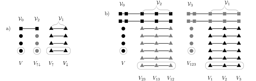
Figure 1: The structure of multiplets in the two-site $O(2)$ (a) and $O(3)$ (b) fermionic chain. Each column depicts a $\sigma$ subspace $V_{a_{1}\dots a_{m}}$ labeled by the odd flavor values. The identical columns unite into a single sector, ${\cal V}_{m}$. The black circles, triangles, and squares represent the singlet, vector, and (traceless) symmetric states, respectively. The gray dots in the listed order denote the pseudo-singlet, pseudo-vector and pseudo-symmetric states. The lines connect the elements of the same multiplet and, hence, are on the same energy level. Each contour encloses the lowest-energy multiplet within the corresponding sector.

In Fig. 1(a), which summarizes the results in Appendix A, the states of the listed multiplets are depicted, respectively, by the black and gray circles, the black triangle, and black square. A line connects the elements of the same multiplet, which, clearly, are on the same energy level.

Each column in Fig. 1 represents a certain $\sigma$ subspace. As we see, the singlets and pseudo-singlets are gathered, respectively, in the even, ${\cal V}_{0}$, and odd, ${\cal V}_{2}$, sectors. At the same time, the vectors compose the remaining sector, ${\cal V}_{1}$. Each vector doublet spreads along the two $\sigma$ subspaces with opposite parities, $V_{\uparrow}$ and $V_{\downarrow}$, which make up that sector.

Every contour encloses the lowest-energy multiplet within the corresponding sector. In the allowed parameter’s region, it is unique. Moreover, we see that in the sector ${\cal V}_{m}$ ($m=0,1,2$) it is characterized by the $m$th-order antisymmetric tensor (the scalar, vector, and pseudoscalar, respectively).

Comparing together the minimal energies of individual sectors [see $E_{0}$ in the expressions (101), (108), and (112) in Appendix A], we conclude that there is no lowest among them for the common coupling parameters (2). In particular, if the latter are restricted by the conditions $g=f$, $e=h$, $r=t$, a degeneracy happens among the sectors ${\cal V}_{0}$ and ${\cal V}_{2}$. Thus, in general, the total ground state may be a unique scalar, a pseudoscalar, a vector doublet, or their superposition.

Go over now to the $O(3)$ model and outline briefly the spectrum properties, derived in detail in Appendix B. The entire space of states, ${\cal V}$, splits into the four sectors, composed of the eight-dimensional $\sigma$ subspaces,

$${\cal V}_{0} =V, {\cal V}_{1} =V_{1}\oplus V_{2}\oplus V_{3},$$ (39)

$${\cal V}_{3} =V_{123},\quad {\cal V}_{2} =V_{12}\oplus V_{13}\oplus V_{23},$$

characterized by the following parities:

$$V_{1} =V_{-++},\quad V_{2} =V_{+-+},\quad V_{3} =V_{++-},$$ (40)

$$V_{12} =V_{--+}, V_{13} =V_{-+-}, V_{23} =V_{+--},$$

$$V =V_{+++}, V_{123} =V_{---}.$$

The $64$-dimensional space ${\cal V}$ is distributed along the four singlets, six vectors, two symmetric traceless tensors (38), depicted again by the black dots (cycles, triangles, squares) in Fig. 1(b), and their pseudo-analogs with the same multiplicities, drawn by the gray dots. Compared to the $O(2)$ case, the two types of new multiplets are listed above: the pseudo-vector, which is equivalent to the antisymmetric tensor $v_{ab}=\sum_{c}\epsilon_{abc}v_{c}$, and the pseudo-analog of the symmetric traceless tensor (38):

$$\psi_{abc}=\sum_{d}\epsilon_{abd}\psi_{dc}.$$ (41)

The latter is more known as a third-order tensor with mixed symmetry Hamermesh . Like the $\psi_{ab}$, it has five independent components.

The distribution of all multiplets along the $\sigma$ subspaces and sectors is shown in Fig. 1(b). In particular, any quintet described by the tensor $\psi_{ab}$ ($\psi_{abc}$) has two states from the sector ${\cal V}_{0}$ (${\cal V}_{3}$), and three others from the sector ${\cal V}_{2}$ (${\cal V}_{1}$), one per each $\sigma$ subspace.

The properties of the lowest-level states are similar to those of the $O(2)$ model. For a given $m=0,1,2,3$, the lowest-energy multiplet of the sector ${\cal V}_{m}$ is a unique $m$th-order antisymmetric tensor (the scalar, vector, pseudovector, and pseudoscalar, respectively).

Again, the total ground state is not determined for the common values of the couplings. In particular, in the case of $g=f$, $e=h$ and $r=t$, a degeneracy emerges among the multiplets and their pseudo-analogs.

The remaining part of the current section is devoted to the extension and proof of the above statement to the $O(N)$ fermionic chains of arbitrary length (1).

III.3 Nonpositive basis

Here we pick up a basis where all nonzero off-diagonal matrix elements of the Hamiltonian become negative. This can be achieved by a specific rearrangement of the fermions in the standard Fock basis, which results in an additional sign factor AL86 ; H10 . First, let us group together the fermions with the same flavors and set them in ascending order by the coordinate. So, define

$$A_{\{x\},a}=c^{+}_{x_{1},a}c^{+}_{x_{2},a}\ldots c^{+}_{x_{n_{a}},a},\qquad x_{1}<\dots<x_{n_{a}},$$ (42)

where $n_{a}$ is the total number of particles with the flavor $a$ in the building state. (In their absence, the above operator is set to unity.) Then define the basic states in the following way:

$$A_{\{x^{1}\},1}A_{\{x^{2}\},2}\ldots A_{\{x^{N}\},N}|0\rangle.$$ (43)

Thus, the particles are arranged first by the flavor numbers, then by the coordinates. In other words, they are displaced in the ascending order in their multi-index values when rewriting the above state in the standard way,

$$\Psi^{x_{1}\dots x_{n}}_{a_{1}\dots a_{n}}=c^{+}_{x_{1},a_{1}}\ldots c^{+}_{x_{n},a_{n}}|0\rangle$$ (44)

with $n=\sum_{a}n_{a}$. The order is defined as

$$(x,a)<(y,b)\quad\text{if}\quad\begin{cases}a<b,\\ a=b\quad\text{and}\quad x<y.\end{cases}$$ (45)

In general, the wave function (44) is not a part of a certain $O(N)$ multiplet apart from the case when all fermions are located on a single site (8), see also Eq. (50) below.

Since the potentials $V$, $\delta V$ are diagonal in the constructed basis, the off-diagonal matrix elements of the chain Hamiltonian are generated exclusively by algebraic combinations of the local operators $K_{x+1\,x}$, $P_{x+1\,x}$ and their conjugates with positive coefficients, see (2), (10), (12), and (13). Therefore, it is enough to show the positivity of the selected basis (43) for the $K,P$ operators.

Indeed, due to the Fermi–Dirac statistics, the hopping term $c^{+}_{x+1,a}c_{x,a}$ acts nontrivially solely on the states with the $a$-type fermion on the $x$th position and without it on the $(x+1)$th one H10 . The resulting action merely replaces the creation operator $c^{+}_{x,a}$ by the annihilation one, $c^{+}_{x+1,a}$. Similarly, a pair annihilation term, $c_{x+1,a}c_{x,a}$, acts nontrivially on the states where both positions are filled with $a$-fermions, which are presented in the basic state (43) in reverse order, $|\dots c^{+}_{x,a}c^{+}_{x+1,a}\dots|0\rangle$. It just eliminates both fermions, producing another basic state without any factor. Clearly, the Hermitian conjugates of both operators, the backward hopping, $c^{+}_{x,a}c_{x+1,a}$, and pair creation, $c^{+}_{x,a}c^{+}_{x+1,a}$, act on the basic states in reverse order. So, all matrix elements of the four considered operators are either $0$ or $1$. Thus the operators $K_{x+1\,x}$, $P_{x+1\,x}$ and their conjugates (13) can generate only integral matrix elements from $0$ to $N$.

The specific fermion ordering in the basic wavefunctions (43) has a simple explanation in terms of the well-known Jordan-Wigner transformation LSM61 ; harada14 . Assigning to each multi-index value the three Pauli matrices, $\tau^{\pm},\tau^{3}$, we get the system of hard-core bosons. Such particles behave alike fermions (bosons) at the same (different) points. Once we have set the ordering (45), the fermions and bosons are related by the Jordan-Wigner transformation:

$$\tau^{\pm}_{x,a}=c^{\pm}_{x,a}\prod_{(y,b)<(x,a)}\sigma_{y,b},\qquad\tau^{3}_{x,a}=-\sigma_{x,a}.$$ (46)

The building blocks of the Hamiltonian (1), expressed in terms of the Pauli matrices, retain their structure:

$$c^{\pm}_{x+1,a}c_{x,a}=-\tau^{\pm}_{x+1,a}\tau^{3}_{x,a}\tau^{-}_{x,a}=\tau^{\pm}_{x+1,a}\tau^{-}_{x,a}.$$ (47)

Using the relations (46), it is easy to see that the multi-fermionic wavefunctions (43) in ascending order (44) can be expressed as multi-bosonic states:

$$\Psi^{x_{1}\dots x_{n}}_{a_{1}\dots a_{n}}=\tau^{+}_{x_{1},a_{1}}\ldots\tau^{+}_{x_{n},a_{n}}|0\rangle.$$ (48)

Evidently, the ordering of Pauli matrices on the right side of this equation is not essential in contrast to the fermion ordering on the left side. Then the relations (10), (12), (13), and (47) reaffirm the nonpositivity of the basis (48).

Finally, note that the basic states keep their form in the Majorana representation too:

$$\Psi^{x_{1}\dots x_{n}}_{a_{1}\dots a_{n}}=\gamma^{(1)}_{x_{1},a_{1}}\ldots\gamma^{(1)}_{x_{n},a_{n}}|0\rangle.$$ (49)

Of course, the Majorana fermions on the right side are in ascending order.

III.4 $O(N)$ structure of relative ground states

In the previous section we have selected a nonpositive basis for the fermionic Hamiltonian (1). In addition, the Hamiltonian connects any two basic elements belonging to an invariant subspace (29). Indeed, manipulating successively with the fermion hoppings $c_{x\pm 1,a}^{+}c_{x,a}$ and pair annihilations $c_{x+1,a}c_{x,a}$, one can easily transfer any target basic state from the subspace $V^{L}_{a_{1}\dots a_{m}}$ to an $m$-particle trial state. All particles there are gathered on the first site of the chain (44):

$$\Psi_{a_{1}\dots a_{m}}=\Psi_{a_{1}\dots a_{m}}^{1\,\dots\,1}.$$ (50)

The above wavefunction transforms as a rank-$m$ antisymmetric tensor under the rotations as already discussed (8).

According to the Perron-Frobenius theorem, the lowest energy state in the invariant subspace $V^{L}_{a_{1}\dots a_{m}}$ (the relative ground state) is nondegenerate. Moreover, it can be expressed as a positive superposition of all basic states (43) inside this subspace (denoted shortly by $\Phi_{\alpha}$):

$$\Omega_{a_{1}\dots a_{m}}=\sum_{\alpha=1}^{2^{N(L-1)}}\omega_{\alpha}\Phi_{\alpha},\qquad\omega_{\alpha}>0.$$ (51)

Since the trial state (50) is a member of this family, one can set $\Phi_{1}=\Psi_{a_{1}\dots a_{m}}$. Due to the rotational symmetry, the relative ground state must be a part of a single $O(N)$ multiplet. Otherwise, it would split into mutually orthogonal pieces, belonging to nonequivalent multiplets. This fact would lead to a spontaneous symmetry breaking in the subspace $V^{L}_{a_{1}\dots a_{m}}$, which contradicts the above proven uniqueness condition. Therefore, state $\Omega_{a_{1}\dots a_{m}}$ has the same $O(N)$ structure as state $\Phi_{1}$ itself: Both wavefunctions belong to different but equivalent multiplets.

In particular, by removing the restriction on the indexes, one can set the lowest state to be antisymmetric alike the trial one,

$$\Omega_{\dots a_{i}\dots a_{j}\dots}=-\Omega_{\dots a_{j}\dots a_{i}\dots}.$$ (52)

Selecting another $m$-combination of the flavors, we arrive at a similar state within the subspace $V^{L}_{b_{1}\dots b_{m}}$. All such subspaces are equivalent as was established in Sec. III.1, mapped to each other by the flavor exchanges (30), and produce together a single degenerate $m$ sector (32).

Summarizing, we come to the conclusion that the lowest energy wavefunction in the sector with $m$ odd flavors, $\mathcal{V}^{L}_{m}$, is given by a single $m$-th order antisymmetric $O(N)$ tensor described by the one-column Young tableau of the same length:

$$\mathbb{Y}_{m}=\mathbb{Y}[1^{m}].$$ (53)

The components provide the nondegenerate relative ground states in the invariant subspaces $V^{L}_{a_{1}\dots a_{m}}$.

Note that according to the representation theory of the orthogonal group Hamermesh , the pair of multiplets, described by the Young diagrams $\mathbb{Y}_{m}$ and $\mathbb{Y}_{N-m}$, are mutually conjugate and related by the Levi-Civita symbol:

$$\Omega^{\prime}_{a_{1}\dots a_{N-m}}=\frac{1}{m!}\sum_{b_{1},\dots,b_{m}}\epsilon_{a_{1}\dots a_{N-m}b_{1}\dots b_{m}}\Omega_{b_{1}\dots b_{m}}.$$ (54)

As $SO(N)$ representations, they are equivalent and characterized by the smallest number among $m$ and $N-m$. Both multiplets are distinguished by the sign under improper rotations, which maps tensor to pseudotensor. One can mention this sign by the prime so that $O(N)$ representations are characterized by the Young diagrams $\mathbb{Y}_{m}$ and

$$\mathbb{Y}_{m}^{\prime}\sim\mathbb{Y}_{N-m}\quad\text{with}\quad m\leq{\textstyle\frac{1}{2}}N$$ (55)

provided that for an even group rank, $\mathbb{Y}_{N/2}\sim\mathbb{Y}^{\prime}_{N/2}$.

For example, the empty diagram is a scalar (singlet) while the single $N$-length column, given by the Levi-Civita tensor, is a pseudoscalar. So, according to our results, in the even-parity sector, $\mathcal{V}^{L}_{0}$, the lowest-level state is a scalar, whereas it is a pseudoscalar in the odd-parity sector, $\mathcal{V}^{L}_{N}$. Similarly, the lowest-level state in the sector with a single odd (even) flavor, $\mathcal{V}^{L}_{1}$ ($\mathcal{V}^{L}_{N-1}$) is a vector (pseudovector).

The relation among the lowest energy levels within the distinct invariant $m$ sectors remains an open question. In particular, the total ground state may coincide with a single antisymmetric multiplest $\mathbb{Y}_{m}$ for some $m$ or it can be an arbitrary combination of them. Below we show that for the particular values of the coupling constants one can achieve the complete degeneracy when the lowest energy levels in all sectors coincide. In that case, the relative ground states (51) from all subspaces $V^{L}_{\sigma_{1}\dots\sigma_{N}}$ form the $2^{N}$-fold completely degenerate total ground state.

III.5 Decoupled Kitaev chains

Consider the chain (1) without the four-fermion interactions where we set also $t_{x}=r_{x}$,

$$H =\sum_{a=1}^{N}H_{a},$$ (56)

$$H_{a} =-\sum_{x=1}^{L-1}t_{x}\big{(}c^{+}_{x+1,a}c_{x,a}+c_{x+1,a}c_{x,a}\,+\text{H.c.}\big{)}.$$

The related Majorana system (24) is reduced to the $N$ decoupled Kitaev chains kitaev01 :

$$H_{a}=-\imath\sum_{x=1}^{L-1}t_{x}\gamma^{(1)}_{x+1,a}\gamma^{(2)}_{x,a}.$$ (57)

In each Hamiltonian, the two boundary Majorana modes, $\gamma^{(1)}_{1,a}$ and $\gamma^{(2)}_{N,a}$, are absent. They produce a single nonlocal fermion, the presence or absence of which does not affect the energy spectrum:

$$\big{[}H,c^{\pm}_{a}\big{]}=0,\qquad c_{a}^{\pm}=\frac{\gamma_{1,a}^{(1)}\mp\imath\gamma_{N,a}^{(2)}}{2}.$$ (58)

One can choose the boundary Majorana fermions, $\gamma_{a}=\gamma_{1,a}^{(1)}$, to implement the mapping between different $\sigma$ subspaces (26), (27). In this case, they also intertwine the Hamiltonian’s action on these subspaces. Therefore, the spectrum in all subspaces $V^{L}_{\sigma_{1}\dots\sigma_{N}}$ are identical. In particular, the ground state completely breaks the $Z_{2}^{\times N}$ symmetry.

IV Particle-hole symmetry in $O(N)$ fermion chain

IV.1 Particle-hole transformation

In this section, we define the particle-hole transformation and study its properties. For a single fermion, which we consider first, the particle-hole map may be described as a similarity transformation induced by the first Majorana fermion (16),

$$\gamma^{(1)}c^{\pm}\gamma^{(1)}=c^{\mp}.$$ (59)

A similar map, provided by the second fermion, produces an additional sign:

$$\gamma^{(2)}c^{\pm}\gamma^{(2)}=-c^{\mp}.$$ (60)

The above maps separate two Majorana modes within a single complex fermion: the first (second) map detects the parity of the second (first) mode.

The transformations (59) and (60) generate a $Z_{2}\times Z_{2}$ group and interchange between the particle and hole, $n\to 1-n$ with $n=0,1$ meaning the fermion number. Their composition gives the parity operator (18), which alters the sign of the creation-annihilation operators:

$$\sigma c^{\pm}\sigma=-c^{\pm},\qquad\sigma=-\imath\gamma^{(1)}\gamma^{(2)}.$$

Get back now to the chain model (1) and apply the last transformation to all fermions located on the odd nodes: $c^{\pm}_{x,a}\to(-1)^{x}c^{\pm}_{x,a}$. As a result, it alters the signs of the double-fermion couplings,

$$t_{x}\to-t_{x},\qquad r_{x}\to-r_{x},$$

without touching the other parts of the Hamiltonian. As a result, the positivity requirement on these coefficients (2) may be weakened by setting the same sign for them:

$$r_{x}t_{x}>0.$$ (61)

Construct now a global particle-hole map for the entire system in a way suitable for our purposes. Apply the transformations (59) and (60) to the even-site and odd-site fermions, respectively. The resulted conjugation is given by the following operator:

$$\hat{\Gamma}=e^{-\imath\varphi}\prod_{x,a}\gamma_{x,a}^{(\lambda_{x})},$$ (62)

where the function $\lambda_{x}$ separates the odd and even coordinates: $\lambda_{\text{odd}}=1$ and $\lambda_{\text{even}}=2$. Although the operator order in the product (62) is not relevant, we set, for definiteness, the ascending order (45). As usual, the phase factor

$$\varphi=\pi{\textstyle\frac{(LN-1)LN}{4}}$$ (63)

is chosen to fulfill the involutivity condition:

$$\hat{\Gamma}^{2}=1.$$ (64)

Thus, the particle-hole operator $\hat{\Gamma}$ generates a $Z_{2}$ group. Obviously, it is unitary, which also ensures the Hermiticity. It (anti)commutes with the Majorana fermion operators,

$$\hat{\Gamma}\gamma^{(\lambda_{x})}_{x,a}\hat{\Gamma} =(-1)^{LN-1}\gamma^{(\lambda_{x})}_{x,a},$$ (65)

$$\hat{\Gamma}\gamma^{(\bar{\lambda}_{x})}_{x,a}\hat{\Gamma} =(-1)^{LN}\gamma^{(\bar{\lambda}_{x})}_{x,a},$$

as well as with the reflection operators, see Eq. (19):

$$\hat{\Gamma}\hat{\sigma}_{a}\hat{\Gamma}=(-1)^{L}\hat{\sigma}_{a}.$$ (66)

In addition, it commutes with the proper rotations (4) or (21):

$$\hat{\Gamma}\hat{L}_{ab}\hat{\Gamma}=\hat{L}_{ab}.$$

The last two equations uncover the $O(N)$ structure of the $\hat{\Gamma}$. It is a scalar for even-length chains and a pseudoscholar for odd lengths.

The global particle-hole map differs by a sign from its local counterparts (59) and (60):

$$\hat{\Gamma}c^{\pm}_{x,a}\hat{\Gamma}=(-1)^{LN-x}c^{\mp}_{x,a}.$$ (67)

It converts the empty state into the completely filled one with the prescribed fermion order (45):

$$\hat{\Gamma}|0\rangle=e^{-\imath\varphi^{\prime}}\prod_{x,a}c^{+}_{x,a}|0\rangle=e^{-\imath\varphi^{\prime}}|\overline{0}\rangle,$$ (68)

$$\varphi^{\prime}=\varphi-\pi{\textstyle\frac{N}{2}\left[\frac{L}{2}\right]}.$$ (69)

Here the barred vacuum means the empty-hole state.

A similar transform of a general basic state (43) produces an additional sign factor, which may be calculated using the relations (67) and (68). In particular, a trial wavefunction (50) converts into the following state:

$$\hat{\Gamma}\Psi_{a_{1}\dots a_{m}}=e^{-\imath\varphi^{\prime}}(-1)^{pL-m}\overline{\Psi}_{a_{1}\dots a_{m}},$$ (70)

$$p=(N-1)m+a_{1}+\dots+a_{m}.$$

Here again, the bar describes a state in terms of the holes rather than particles. So, the state $\overline{\Psi}_{a_{1}\dots a_{m}}$ contains the ordered fermions, all except those having the flavors $a_{1},\dots,a_{m}$ and located on the first node:

$$\overline{\Psi}_{a_{1}\dots a_{m}}=\prod_{(x,a)\neq(1,a_{i})}c^{+}_{x,a}|0\rangle.$$ (71)

It is a member of the basis (43), or (44).

In general, any basic state $\Psi^{x_{1}\dots x_{n}}_{a_{1}\dots a_{n}}$ has its counterpart $\overline{\Psi}^{x_{1}\dots x_{n}}_{a_{1}\dots a_{n}}$ with the holes instead of particles. Clearly, there is no a $\hat{\Gamma}$-invariant state, so the entire basis splits into $2^{NL-1}$ such pairs.

We remark that an equivalent particle-hole operator may be introduced by applying the alternating local maps (59) and (60) in reverse order (see Ref. Wei15 for the $N=1$ case):

$$\hat{\Gamma}^{\prime}=e^{-\imath\varphi}\prod_{x,a}\gamma_{x,a}^{(\bar{\lambda}_{x})}.$$ (72)

Both matrices are related to each other through the total fermion parity $\hat{\sigma}=\prod_{a=1}^{N}\hat{\sigma}_{a}$:

$$\hat{\Gamma}\hat{\Gamma}^{\prime} =\hat{\Gamma}^{\prime}\hat{\Gamma}=\hat{\sigma}\quad\text{for even $NL$},$$

$$\hat{\Gamma}\hat{\Gamma}^{\prime} =-\hat{\Gamma}^{\prime}\hat{\Gamma}=\imath\hat{\sigma}\quad\text{for odd $NL$}.$$

IV.2 Particle-hole symmetric $O(N)$ chains

Remember that in Sec. III.4 the $O(N)$ structure and degeneracy of the lowest energy states of the fermionic model (1) is revealed. Here we consider the behavior of these wavefunctions under the additional $Z_{2}$ (particle-hole) symmetry.

The particular choice, which distinguishes between the even and odd sites (62), implies the invariance of the local Hamiltonian (12), modified by the replacement:

$$P_{yx}^{+}P_{yx} \to\frac{1}{2}(P_{yx}^{+}P_{yx}+P_{yx}P_{yx}^{+}),$$ (73)

$$K_{yx}^{+}K_{yx} \to\frac{1}{2}(K_{yx}^{+}K_{yx}+K_{yx}K_{yx}^{+}).$$

Indeed, the relations (65) and Majorana fermion representations of the $K,P$ operators (22), (23) imply

$$\hat{\Gamma}\begin{pmatrix}K_{x+1,x}\\ P_{x+1,x}\end{pmatrix}\hat{\Gamma}=\begin{pmatrix}K_{x+1,x}^{+}\\ P_{x+1,x}^{+}\end{pmatrix}.$$ (74)

Note that from the commutation relations (14), it becomes clear that the above modification (73) results in an extra chemical potential,

$$\delta V^{\prime}=\sum_{x=1}^{L-1}(g_{x}+f_{x})n_{x}+(g_{x}-f_{x})n_{x+1},$$

which may be absorbed by the potential.

From the other side, the modified potential (11) is not symmetric and undergoes the following shift:

$$\hat{\Gamma}V^{\prime}(\dots,n_{x},\dots)\hat{\Gamma}=V^{\prime}(\dots,N-n_{x},\dots).$$

Consider now the potentials which remain invariant under the particle-hole transformation:

$$V^{\prime}(n_{1},\dots,n_{L})=V^{\prime}(N-n_{1},\dots,N-n_{L}).$$

This happens, for example, when they depend on the products $(N-n_{x})n_{x}$ as in the case of the $SU(N)$ Hubbard potential. Therefore, the respective Hamiltonians are also preserved, as can be inferred from the relations (10), (12), and (74):

$$[\hat{\Gamma},H]=0.$$

The particle-hole structure of the relative ground states manifests a parity effect on the chain’s size.

For even-length chains, $L=2l$, the particle-hole and reflection symmetries are compatible according to the relation (66):

$$[\hat{\Gamma},\hat{\sigma}_{a}]=0.$$

Together they constitute a discrete group $Z_{2}^{\times(N+1)}$, which preserves any individual $\sigma$ subspace. Due to the uniqueness condition established in Sec. III.4, the relative ground state also remains invariant under the particle-hole symmetry. To detect the corresponding quantum number, we observe that the basic states meet in pairs in the decomposition (51). The pair members are related by the particle-hole map such as, in particular, the two paired states, (50) and (71). The phase factor in the definition of $\hat{\Gamma}$ (69) is trivial, $\varphi^{\prime}=\pi(Nl-1)Nl$, and Eq. (70) simplifies to the following one:

$$\hat{\Gamma}\Psi_{a_{1}\dots a_{m}}=(-1)^{m}\overline{\Psi}_{a_{1}\dots a_{m}}.$$ (75)

Both states participate in the sum (51) with positive coefficients, which have to equal, giving rise to a combined state $\Psi_{a_{1}\dots a_{m}}+\overline{\Psi}_{a_{1}\dots a_{m}}$ with the particle-hole parity $(-1)^{m}$. Clearly, it coincides with the eigenvalue of the relative ground state (51):

$$\hat{\Gamma}\Omega_{a_{1}\dots a_{m}}=(-1)^{m}\Omega_{a_{1}\dots a_{m}}.$$ (76)

For odd-length chains, $L=2l-1$, the particle-hole transformation anticommutes with reflections (66),

$$\{\hat{\Gamma},\hat{\sigma}_{a}\}=0.$$ (77)

This fact leads to the additional twofold degeneracy of the energy levels. Indeed, the particle-hole transformation inverts the parities of all flavors. It matches the Hamiltonian’s spectrum on the two invariant $\sigma$ subspaces (25):

$$\hat{\Gamma}V^{L}_{\sigma_{1}\dots\sigma_{N}}=V^{L}_{-\sigma_{1}\dots-\sigma_{N}}.$$

Therefore, both subspaces have identical spectra. As a consequence, the two invariant sectors are degenerate (32),

$$\hat{\Gamma}{\cal V}^{L}_{m}={\cal V}^{L}_{N-m}.$$

The exclusion is the sector with $m=N/2$ for even values of the group rank $N$. The double degeneracy occurs within the sector ${\cal V}^{L}_{N/2}$ containing an equal number of flavors with odd and even parities.

V Further extensions and spin chains

The result on the nondegeneracy and the multiplet structure of the relative ground state, obtained in the previous section, remain valid for more general class of $SO(N)$ invariant fermionic chains. Recall that the local Hamiltonian (12) is constructed from the blocks (13) using negative numbers to prevent any positive off-diagonal matrix element in the selected basis (43). In fact, more members can be added just keeping this rule.

Note that the four-particle interactions in the original Hamiltonian (1) are chosen to preserve the number of fermions of each sort, $n_{a}$. The requirement simplifies the system but is not necessary. Thus, the interaction $K_{xy}P^{+}_{xy}$ with the conjugate can also be included in the local Hamiltonian (12). They are responsible for a particle decay into three particles and the reverse process.

V.1 Long-range interactions

So far, we have deal with the nearest-neighbor interaction in the open fermionic chain. The building blocks of the Hamiltonian (13), which couple two distant sites, are not yet positive in the basis (48). The simple replacement of the fermionic operators with their bosonic counterparts given by the Pauli matrices (47) is not valid for a distant interaction any more. Instead, the Jordan-Wigner transformation (46) imply a nonlocal coupling between distant sites, depending on the overall fermionic parity in all intermediate positions. To avoid a sign problem, we redefine them in the following way:

$$K_{yx}=\sum_{a}\tau^{+}_{y,a}\tau^{-}_{x,a}=\sum_{a}c^{+}_{y,a}c_{x,a}\prod_{x<z<y}\sigma_{z,a},$$ (78)

$$P_{yx}=\sum_{a}\tau^{-}_{y,a}\tau^{-}_{x,a}=\sum_{a}c_{y,a}c_{x,a}\prod_{x<z<y}\sigma_{z,a}.$$

Clearly, all results about the relative ground states and their multiplet structure, established for the open chains, remain valid for an analog of the Hamiltonian (10) with the long-range interactions:

$$\hat{H}_{\text{lr}}=\sum_{x<y}\left(H_{yx}+H_{yx}^{+}\right)+V^{\prime}(n_{1},\dots,n_{L}).$$ (79)

The interaction between two distant sites depends on positive coupling constants, as in the adjacent case (12):

$$H_{yx}= -t_{yx}K_{yx}-r_{yx}P_{yx}-f_{yx}K_{yx}K_{yx}^{+}$$ (80)

$$-g_{yx}P_{yx}^{+}P_{yx}-h_{yx}K_{yx}^{2}-e_{yx}P_{yx}^{2}.$$

V.2 Cyclic boundaries and translation invariance

Let us restrict the distant interactions to a single term binding together the first and last sites. As a result, the nearest-neighboring chain (10) is supplemented by the cyclic boundary term,

$$\hat{H}_{\text{cyc}}=\hat{H}+H_{\text{b}},\qquad H_{\text{b}}=H_{L1}+H_{L1}^{+}.$$ (81)

As soon as this term is borrowed from the long-range interacting model (80), it fulfills the sign rule. It is easy to observe that the sign factors, depending on the intermediate fermions, are provided by the total parity operators (78),

$$K_{L1}=-\sum_{a}c^{+}_{L,a}c_{1,a}\hat{\sigma}_{a},\quad P_{L1}=-\sum_{a}c_{1,a}c_{L,a}\hat{\sigma}_{a},$$ (82)

which take constant values, $\sigma_{a}$, on the invariant subspaces $V^{L}_{\sigma_{1}\dots\sigma_{N}}$. Thus, the boundary conditions depend on the individual $\sigma$ subspaces. Below we consider only one of them.

Define the elementary lattice translation:

$$\hat{T}c^{\pm}_{x,a}\hat{T}^{-1}=c^{\pm}_{x(\text{mod}\,L)+1,a}.$$ (83)

Its eigenvalues $e^{ip}$ are given by the lattice momentum values, $p=0,{\textstyle\frac{2\pi}{L}},\dots,{\textstyle\frac{2\pi(L-1)}{L}}$. Evidently, it commutes with the $O(N)$ symmetry, including the parity operators:

$$[\hat{T},\hat{\sigma}_{a}]=0.$$ (84)

Let us confine the Hamiltonian to the odd-parity sector, ${\cal V}^{L}_{N}=V^{L}_{-\dots-}$, and consider the site-independent coupling constants (2):

$$r_{x}=r,\quad t_{x}=t,\quad f_{x}=f,\quad\text{etc.}$$

Then the translation operator maps the local Hamiltonians to each other, including the boundary one (81). This property ensures the translation invariance of the restricted system,

$$\hat{T}H_{x\,x-1}\hat{T}^{-1}=H_{x+1\,x},\qquad[\hat{T},\hat{H}_{\text{cyc}}]=0,$$

with the $x\pm 1$ taken on modulo $L$ [see Eq. (83)].

We affirm that the relative ground state of the translation-invariant Hamiltonian in the odd-parity sector, $\sigma_{a}=-1$, is a pseudoscalar with zero momentum:

$$\hat{T}\Omega_{12\dots N}=\Omega_{12\dots N}.$$ (85)

One can use arguments similar to those in the proof of Eq. (76). Using the translations, circulate the trial state (50) to all nodes and take the sum to get a translation-invariant state with zero momentum:

$$\Psi=\sum_{l=0}^{L-1}\hat{T}^{l}\Psi_{12\dots N},\qquad\hat{T}\Psi=\Psi.$$ (86)

It is easy to observe that the above state takes part in the linear combination (51). Due to the uniqueness condition, the both states, $\Omega_{12\dots N}$ and $\Psi$, have the same momentum quantum number, which proves the equation (85).

Note that for the even-size chains with odd Majorana modes per site (which is not our case with the $2N$ modes), the commutator in Eq. (84) is replaced by the anticommutator. As a result, the twofold degeneracy appears with the supersymmetry behind it super . This resembles a similar behavior (without a supersymmetry) in the case of the particle-hole symmetry and odd-size chains [see Sec. IV.2, Eq. (77)].

V.3 Mixed-spin chains

The six and more fermion exchange terms may also contribute in the local interaction. Among them there are the second- and higher-order $SO(N)$ Heisenberg spin exchanges.

Consider the limiting case when all other terms are absent so that the Hamiltonian acquires the following form:

$$\hat{H}_{\text{s}}=\sum_{x}\left(J^{(1)}_{x}\bm{L}_{x+1}\cdot\bm{L}_{x}-J^{(2)}_{x}(\bm{L}_{x+1}\cdot\bm{L}_{x})^{2}\right),$$ (87)

where higher powers, $k<N$, of the Heisenberg exchange (15) may be involved too. In order to fulfill the required sign rule, they must be with alternating couplings:

$$(-1)^{k-1}J^{(k)}_{x}\qquad\text{with}\qquad J^{(k)}_{x}>0.$$ (88)

The positivity condition may be weakened (see, for example, the inequality (93) for the second coupling below).

In fact, it is easy to check that the local spin-exchange interaction (15) is purely off-diagonal and may be presented in the form,

$$\bm{L}_{y}\cdot\bm{L}_{x}=-\sum_{a\neq b}\left(c^{+}_{x,a}c_{y,a}c^{+}_{y,b}c_{x,b}+c^{+}_{x,a}c^{+}_{y,a}c_{y,b}c_{x,b}\right)$$ (89)

with $y=x+1$. This expression is built from the double-fermion operators with the same flavor, like $c^{+}_{x,a}c_{y,a}$. As was derived already in Sec. III.3, they produce non-negative matrices in the current basis. As a result, all matrix elements of $\bm{L}_{x+1}\cdot\bm{L}_{x}$ are nonpositive.

Clearly, the Hamiltonian (87) keeps unchanged the local intrinsic spins given by the antisymmetric representations $\mathbb{Y}_{m_{x}}$ and the total number of fermions per site:

$$[\hat{H}_{\text{s}},n_{x}]=0.$$

Thus, it has a block diagonal form with $L^{N+1}$ parts, according to all possible distributions of the local fermion numbers $n_{x}=m_{x}=0,\dots,N$ along the chain nodes. Moreover, the trivial representations, $m_{x}=0,N$, appearing anywhere, cut the chain into the two disjoint pieces. We get in this way a set of the mixed-spin chains containing no more than $L$ nodes. Each site is endowed with an $O(N)$ antisymmetric multiplet (higher spin) $\mathbb{Y}_{m}$ formed by $n_{x}=m_{x}$ fermions provided that

$$1\leq m_{x}\leq N-1.$$ (90)

The particle-hole transformation $\hat{\Gamma}$ (59) intertwines between two ”dual” chains composed from the mutually conjugate representations with $m_{x}$ and $N-m_{x}$ fermions per node, ensuring the equivalence of both Hamiltonians.

Select now a single chain from this family and keep the notations (for the length, invariant sectors, the lowest level states there, etc.) the same to avoid new entries. Clearly, the total amount of fermions and the total parity $\hat{\sigma}=(-1)^{\hat{n}}$ take constant values therein:

$$n =\sum_{a=1}^{N}n_{a}=\sum_{x=1}^{L}m_{x},$$

$$\sigma =\prod_{a=1}^{N}\sigma_{a}=\prod_{x=1}^{L}(-1)^{m_{x}}.$$

As a result, the reflection symmetry for spin chains is reduced to the $Z^{\times(N-1)}$ group composed from $N-1$ independent parities H15 .

Hence, the allowed invariant sectors $\mathcal{V}^{L}_{m}$ (32) have to obey the parity rule:

$$(-1)^{m}=\sigma=(-1)^{n}.$$ (91)

Of course, they are still $\binom{N}{m}$-fold degenerate, but their dimensions are essentially less comparing with those in the parent, fermionic chain. Note that a single Majorana fermion $\gamma_{a}$ alters the total parity value, taking beyond the spin chain’s space of states. Therefore, the equivalence relation between two $\sigma$ subspaces (26) is not valid any more. Moreover, their dimensions differ in general.

Figure 2 illustrates a sample mixed-spin chain with $N=5$ flavors. The (higher) spins on the nodes are members of the antisymmetric multiplets $\mathbb{Y}_{m}$ with $m=2,1,3,4,2$ fermions per site. Their dimensions are listed at the bottom. For a conjugate pair $\mathbb{Y}_{1},\mathbb{Y}^{\prime}_{1}$ or $\mathbb{Y}_{2},\mathbb{Y}^{\prime}_{2}$ (55), they coincide so the representations $\mathbb{Y}^{\prime}_{1,2}$ are plotted in gray and marked with an overbar.

A sample state is displayed in terms of the Young tableau at the top: a box means a fermion with inscribed flavor Hamermesh . Using the comma to separate the adjacent nodes apart, it may be written as follows:

$$\ket{34,2,1245,235,12}\!=c^{+}_{1,3}c^{+}_{1,4}c^{+}_{2,2}\dots\dots c^{+}_{5,2}\ket{0}\!.$$ (92)

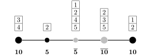
Figure 2: The five-site mixed-spin chain with $O(5)$ symmetry with $x$th node filled by the $m_{x}$ fermions. The related antisymmetric multiplet is characterized by its dimension $\binom{5}{m}$ with or without the bar listed below. The bar (and gray color) marks a multiplet $m^{\prime}=3,4$ dual to that with $m=5-m^{\prime}$, A particular state (92) is shown with the flavors inside the boxes atop.

In the particular case when each node of the system (87) is occupied by a single fermion, $m_{x}=1$, we arrive at the $SO(N)$ invariant spin chain in the vector (defining) representation, already considered in the current context harada14 ; H15 . Following the common parity rule (91), the total parity must equal the length’s parity:

$$(-1)^{m}=\sigma=(-1)^{L}.$$

Rearranging fermions according to their positions as done above (92), we present the related fermionic basis (43) in a form more conventional for spin systems (commas are omitted):

$$|a_{1}\dots a_{L}\rangle=(-1)^{p_{a_{1}\dots a_{L}}}c^{+}_{1,a_{1}}\dots c^{+}_{L,a_{L}}|0\rangle.$$

Here $p_{a_{1}\dots a_{L}}$ is a number of disordered pairs is the sequence, i.e., the amount of the flavor pairs with $x<y$ but $a_{x}>a_{y}$.

The local spin exchange (89) produces on the above state:

$$\bm{L}_{x+1}\cdot\bm{L}_{x}\,|ab\rangle=(-1)^{1-\delta_{ab}}|ba\rangle-\delta_{ab}\sum_{c}|cc\rangle.$$

Here only the spins at the neighboring $x$th and $(x+1)$th positions are mentioned, the others are not affected and omitted. As was already discussed, it contains solely negative elements out of the diagonal. Therefore, its square has positive matrix elements:

$$(\bm{L}_{x+1}\cdot\bm{L}_{x})^{2}|ab\rangle=|ab\rangle+(N-2)\delta_{ab}\sum_{c}|cc\rangle$$

(the angular momentum exists merely for $N\geq 2$).

The assembly of the common terms in both operators broadens the definition area of the second coupling (88) beyond the positive region H15 :

$$J_{x}^{(2)}>-\frac{J_{x}^{(1)}}{N-2}.$$ (93)

It contains the integrable point,

$$J^{(2)}=-\frac{N-4}{(N-2)^{2}}J^{(1)},$$ (94)

at which the translational invariant system is solved exactly by the Bethe ansatz resh .

One can spread out the results in Sec. III.4 to the spin chain system. In particular, the ground state in the sector $\mathcal{V}^{L}_{m}$ is given by a single $m$-th order antisymmetric $O(N)$ tensor with the components $\Omega_{a_{1}\dots a_{m}}$, producing the unique relative ground states in the subspaces $V^{L}_{a_{1}\dots a_{m}}$.

The proof repeats the steps for the parent model from Sec. III. The connectivity of the spin Hamiltonian (87) in the nonpositive basis (44) inside a restricted $\sigma$ subspace is easy to establish using the representation (15). Due to the uniqueness and continuity, the multiplet type of the relative ground state remains unchanged along the path connecting the Hamiltonians (1) and (87). Alternatively, one can look for a more complex trial wavefunction than the state (50), which may go beyond the space of the spin chain states, see Refs. H10 ; H15 . For instance, one can set

$$\Psi_{a_{1}\dots a_{m}}=\sum_{s}\Psi_{a_{1}\dots a_{m}}^{x_{s_{1}}\dots x_{s_{m}}},$$ (95)

where the sum is taken over the nontrivial permutations of a chosen coordinate set $x_{1},\dots,x_{m}$. It is easy to see that the above wavefunction is antisymmetric in the flavors.

VI Conclusion

We have studied the properties of the sectoral ground states (degeneracy, multiplet structure) of the $O(N)$ invariant finite-size chain of interacting (Dirac or Majorana) fermions with $N$ spins (flavors).

The system does not retain the number of particles with a given flavor $a$ but keeps its parity, $\sigma_{a}$. The corresponding invariant subspaces $V_{a_{1}\dots a_{m}}$ labeled by the values of odd flavors (that is, the flavors with $\sigma_{a}=-1$), are related with each other by the Majorana modes and thus have the same dimension. In general, they differ in their spectrum. Merely the $\sigma$ subspaces with the same number $m$ of odd flavors are completely degenerate and unified into a single invariant $m$ sector.

For a wide range of coupling constants, we have established in the current paper that the lowest energy $O(N)$ multiplet in any such $m$ sector is unique and represented by an $m$th-order antisymmetric tensor, $\Omega_{a_{1}\dots a_{m}}$. Owing to the degeneracy, its components are the unique lowest energy states (the relative ground states) in the subspace $V_{a_{1}\dots a_{m}}$.

Note that there is no way to somehow relate the lowest levels of two distinct sectors. In fact, the exact results in the two-site samples and Kitaev chain illustrate that there is not any ordering between them for common parameters. The additional degeneracies may happen at special values of couplings, including the complete degeneracy among all $N+1$ sectors.

Such degeneracies usually emerge in the presence of extra symmetries as the particle-hole symmetry. The impact on the spectrum depends on the parity of the chain’s size. For the even-length chains, the particle-hole and $O(N)$ symmetries commute. This endows the ground states $\Omega_{a_{1}\dots a_{m}}$ with an additional parity given by the particle-hole eigenvalue, $(-1)^{m}$. For the odd length chains, the particle-hole map does not commute with improper rotations any more. Instead, it alters the values of all parities, leading to an additional twofold degeneracy between the dual subspaces $V_{a_{1}\dots a_{m}}$ and $V_{a^{\prime}_{1}\dots a^{\prime}_{N-m}}$ with differing flavor sets $a_{i}$ and $a^{\prime}_{i}$.

Remember that for the $U(N)$ fermionic chain, there is no a particle creation-annihilation process, so the fermion quantum numbers per flavor, $n_{a}$, are good and mark the invariant subspaces. The subspaces with the same total number, $n=\sum_{a}n_{a}$, are combined into the sectors. It is known that the lowest-energy states in each such $n$-sector is described by a unique $m$th-order antisymmetric $U(N)$ multiplet with $m=n\mod N$ H10 .

The above results remain valid in the presence of the long-range interactions multiplied by a Jordan-Wigner string. For the translation-invariant system, they are verified merely in the odd-parity sector, $m=N$, where the momentum quantum number of the ground state vanishes.

Finally, the aforementioned statements for the fermionic models have been transferred as well to the $O(N)$ invariant, polynomial Heisenberg chains with alternating couplings and mixed spins. This system is obtained in the limit when the fermion numbers (but not the flavors) per each site persist. They set ranks of the antisymmetric multiplets, where the local spins live. Note that now the number of odd flavors ($m$) in each invariant subspace $V_{a_{1}\dots a_{m}}$ is confined by the total number of fermions: both must have the same parity. The obtained results extend those for the bilinear-biquadratic model in the vector representation H15 .

Appendix A Two-site $O(2)$ fermionic chain

In the current Appendix we derive exactly the spectrum and quantum numbers of the particle-hole invariant two-site $O(2)$ fermionic chain (34), (35). The obtained results have been described briefly in Sec. III.2.

The space of states decomposes into the invariant sectors ${\cal V}_{m}$ with $m=0,1,2$ (36), (37). Here we consider each sector separately.

A.1 $m=0$ sector

The sector ${\cal V}_{0}$ with even particle numbers is spanned by the states

$$\ket{0}\!,\qquad\ket{\uparrow\downarrow,\uparrow\downarrow}\!,\qquad\ket{\uparrow,\uparrow}\!,\qquad\ket{\downarrow,\downarrow}\!,$$ (96)

with a comma separating the nodes, see also the wavefunction (92). We use here the conventional basis where the fermion’s position prevails over the spin. Three states obey the non-positivity condition (42), (43) while the fully occupied state,

$$\ket{\uparrow\downarrow,\uparrow\downarrow}\!=c^{+}_{1,\uparrow}c^{+}_{1,\downarrow}c^{+}_{2,\uparrow}c^{+}_{2,\downarrow}\ket{0}\!,$$

needs a sign.

The particle-hole transformation (62) shuffles the states as follows (see also Appendix B.5):

$$\hat{\Gamma}\ket{0}\!=-\ket{\uparrow\downarrow,\uparrow\downarrow}\!,\qquad\hat{\Gamma}\ket{\uparrow,\uparrow}\!=\ket{\downarrow,\downarrow}\!.$$ (97)

Due to the Pauli exclusion principle, the fermion hopping is banned here ($K=0$) while the annihilation of a fermion pair is allowed only on the following states:

$$\begin{gathered}P\ket{\uparrow\downarrow,\uparrow\downarrow}\!=-\ket{\uparrow,\uparrow}\!-\ket{\downarrow,\downarrow}\!,\\ P\ket{\uparrow,\uparrow}\!=P\ket{\downarrow,\downarrow}\!=\ket{0}\!.\end{gathered}$$ (98)

The $O(2)$ symmetry splits the Hamiltonian into two diagonal blocks. The first block,

$$H=\begin{pmatrix}-2g&2e&-\sqrt{2}r\\ 2e&-2g&\sqrt{2}r\\ -\sqrt{2}r&\sqrt{2}r&-4g\end{pmatrix},$$

is spanned by the pure singlets:

$$\ket{0}\!,\qquad\ket{\uparrow\downarrow,\uparrow\downarrow}\!,\qquad{\textstyle\frac{1}{\sqrt{2}}}\left(\ket{\uparrow,\uparrow}\!+\ket{\downarrow,\downarrow}\!\right).$$ (99)

Note that the last one is specific for the orthogonal groups. It forms a trace which contracts the spins of neighboring fermions with the invariant metrics, $\delta_{ab}$. The traceless part of the symmetric tensor (38) makes up an $O(2)$ doublet, one member of which,

$${\textstyle\frac{1}{\sqrt{2}}}\left(\ket{\uparrow,\uparrow}\!-\ket{\downarrow,\downarrow}\!\right),$$ (100)

forms the second block with $H=0$. [The second member belongs to the odd parity sector described below by Eq. (107)].

As a result, the energy eigenvalues are given by the following expressions,

$$E_{0,1}=-e-3g\mp\sqrt{(e-g)^{2}+4r^{2}},$$ (101)

$$E_{2}=2(e-g),\qquad E_{3}=0.$$

Clearly, the lowest level, $E_{0}$ (top sign), is unique in the region with positive parameters.

The relative ground state (51) is a singlet with the following coordinates in the basis (99):

$$\Omega=(\omega,-\omega,1),\qquad\omega={\textstyle\frac{e-g+\sqrt{(e-g)^{2}+4r^{2}}}{2\sqrt{2}r}}.$$

Clearly, $\omega>0$, so its coefficients in the basis (43) become positive in complete agreement with the most common formula (51).

The particle-pole parity is even, as is easy to see for the relations (97),

$$\hat{\Gamma}\Omega=\Omega,$$ (102)

which agrees with the general formula (76).

A.2 $m=2$ sector

The sector ${\cal V}_{2}$ with odd parities is spanned by two fermions with opposite spins:

$$\ket{\uparrow,\downarrow}\!,\qquad\ket{\downarrow,\uparrow}\!,\qquad\ket{\uparrow\downarrow,0}\!,\qquad\ket{0,\uparrow\downarrow}\!.$$ (103)

Note that merely the second state has a wrong sign to make up a nonpositive state (43). The particle-hole inversion (62) produces

$$\hat{\Gamma}\ket{\uparrow,\downarrow}\!=-\ket{\downarrow,\uparrow}\!,\qquad\hat{\Gamma}\ket{\uparrow\downarrow,0}\!=\ket{0,\uparrow\downarrow}\!.$$ (104)

In contrast to the previous sector, here the annihilation is forbidden, $P=0$, and the particle motion conforms to the forward jumps,

$$K\ket{\uparrow\downarrow,0}\!=\ket{\uparrow,\downarrow}\!-\ket{\downarrow,\uparrow}\!,$$ (105)

$$K\ket{\uparrow,\downarrow}\!=-K\ket{\downarrow,\uparrow}\!=\ket{0,\uparrow\downarrow}\!,$$

together with their backwards.

Make use of the $O(2)$ invariance again and split the Hamiltonian into two independent parts. The first block is built on the pseudoscalar sector,

$${\textstyle\frac{1}{\sqrt{2}}}\left(\ket{\uparrow,\downarrow}\!-\ket{\downarrow,\uparrow}\!\right),\qquad\ket{\uparrow\downarrow,0}\!,\qquad\ket{0,\uparrow\downarrow}\!,$$ (106)

with the following matrix,

$$H=-\begin{pmatrix}4f&\sqrt{2}t&\sqrt{2}t\\ \sqrt{2}t&2f&2h\\ \sqrt{2}t&2h&2f\end{pmatrix}.$$

The symmetric combination,

$${\textstyle\frac{1}{\sqrt{2}}}\left(\ket{\uparrow,\downarrow}\!+\ket{\downarrow,\uparrow}\!\right),$$ (107)

is a zero-energy eigenstate. Together with the state (100), it forms an $O(2)$ doublet described by the two-component tensor (38).

Thus, the resulting energy levels are,

$$E_{0,1}=-h-3f\mp\sqrt{(f-h)^{2}+4t^{2}},$$ (108)

$$E_{2}=2(h-f),\qquad E_{3}=0.$$

Clearly, the lowest value, $E_{0}$, is unique in the region with positive parameters. The corresponding state is a pseudo-singlet with the following coordinates in the basis (106):

$$\Omega_{\uparrow\downarrow}=(\omega,1,1),\qquad\omega={\textstyle\frac{f-h+\sqrt{(f-h)^{2}+4t^{2}}}{\sqrt{2}t}}.$$

Since $\omega>0$, all coefficients in the basis (43) are positive in agreement with the general rule (51), as is easy to verity. Its particle-pole parity is even,

$$\hat{\Gamma}\Omega_{\uparrow\downarrow}=\Omega_{\uparrow\downarrow},$$

which follows from Eqs. (104). This fact agrees with the general formula (76).

A.3 $m=1$ sector

The sector ${\cal V}_{1}$ with mixed parities consists of the two $\sigma$ subspaces: $V_{\uparrow}$ and $V_{\downarrow}$ (36), spanned, correspondingly, by the first and second rows below:

$$\ket{\uparrow,0}\!,\qquad\ket{0,\uparrow}\!,\quad-\ket{\downarrow,\uparrow\downarrow}\!, \quad\ket{\uparrow\downarrow,\downarrow}\!,$$ (109)

$$\ket{\downarrow,0}\!,\qquad\ket{0,\downarrow}\!,\qquad\ket{\uparrow,\uparrow\downarrow}\!, -\ket{\uparrow\downarrow,\uparrow}\!.$$ (110)

It is easy to see that every column forms a vector doublet, and the upper component goes to the down one under the $\pi$ rotation.

The Hamiltonian (34) is given by the same matrix in both subspaces, $V_{\uparrow}$ and $V_{\downarrow}$:

$$H=-\begin{pmatrix}f+g&t&0&r\\ t&f+g&r&0\\ 0&r&f+g&t\\ r&0&t&f+g\end{pmatrix}.$$ (111)

This fact reflects the degeneracy and can be also verified using the action of the $K,P$ operators (and their Hermitian conjugates). The nonvanishing processes on $V_{\uparrow}$ are provided by

$$K\ket{\uparrow,0} =\ket{0,\uparrow}\!,\quad K\ket{\downarrow,\uparrow\downarrow} =-\ket{0,\uparrow}\!,$$

$$P\ket{\downarrow,\uparrow\downarrow} =-\ket{0,\uparrow}\!,\quad P\ket{\uparrow\downarrow,\downarrow} =\ket{\uparrow,0}\!,$$

together with their backwards.

The corresponding energy levels are pretty simple:

$$E_{0,1,2,3}=-f-g\mp r\mp t.$$ (112)

Obviously, the lowest level, $E_{0}$ (with minus signs), is unique in the subspace $V_{\uparrow}$ ($V_{\downarrow}$).

The relative ground states in both subspaces have the same expansion,

$$\Omega_{\uparrow}=\Omega_{\downarrow}=(1,1,1,1).$$ (113)

Clearly, both components form a vector doublet, $\Omega_{a}$. The eight basic states (109), (110) match the nonpositivity condition (43), and the unit coefficients justify the most common decomposition formula (51).

Note that simple expressions for the spectrum and eigenstates are the consequence of the lattice reflection and particle-hole symmetries of the Hamiltonian (34). Both of them shuffle the basic states (109), (110). The lowest-energy state is even under the lattice reflection and is odd under the particle-hole transformation:

$$\hat{\Gamma}\Omega_{a}=-\Omega_{a}.$$

The last fact is in agreement with the general rule (76) and can be verified independently applying

$$\hat{\Gamma}\ket{\uparrow,0} =\ket{\downarrow,\uparrow\downarrow}\!,\quad \hat{\Gamma}\ket{0,\uparrow} =-\ket{\uparrow\downarrow,\downarrow}\!,$$

$$\hat{\Gamma}\ket{\downarrow,0} =-\ket{\uparrow,\uparrow\downarrow}\!,\quad \hat{\Gamma}\ket{0,\downarrow} =\ket{\uparrow\downarrow,\uparrow}\!$$

and taking into account the involutivity property (64).

Appendix B Two-site $O(3)$ fermionic chain

Here we derive exactly the spectrum and quantum numbers of the particle-hole invariant two-site $O(3)$ fermionic chain (34), (35). The obtained results have been discussed briefly in Sec. III.2.

The space of states decomposes into the invariant sectors ${\cal V}_{m}$ with $m=0,1,2,3$ (39), (40). Below we treat each sector separately.

B.1 $m=0$ sector

The sector with even parities, ${\cal V}_{0}$, is formed by the following eight states (no summation),

$$\ket{0}\!,\quad\ket{a,a}\!,\quad-\ket{ab,ab}\!,\quad-\ket{123,123}\!,$$ (114)

where $a,b=1,2,3$ and $a<b$. We continue with the Dirac notations from the previous section with the comma separating the nodes. The minus signs has been set to fit the nonpositivity condition (43).

Due to the Pauli exclusion principle, a particle hopping is forbidden here ($K=0$) while the pair annihilation is subjected to the rule,

$$\begin{gathered}P\ket{a,a}\!=\ket{0}\!,\quad P\ket{ab,ab}\!=-\ket{a,a}\!-\ket{b,b}\!,\\ P\ket{123,123}\!=\sum_{a<b}\ket{ab,ab}\!.\end{gathered}$$

The Hamiltonian is split into two blocks, each involving equivalent multiplets. The first block is made from the scalars (singlets), which we endow with the following basis,

$$\ket{0}\!,\quad\sum_{a}\frac{\ket{a,a}\!}{\sqrt{3}},\quad-\sum_{a<b}\frac{\ket{ab,ab}\!}{\sqrt{3}},\quad-\ket{123,123}\!.$$ (115)

Inserting the structure of the $K,P$ operators into the Hamiltonian (34), we obtain:

$$H=-\begin{pmatrix}3g&\sqrt{3}r&2\sqrt{3}e&0\\ \sqrt{3}r&7g&2r&2\sqrt{3}e\\ 2\sqrt{3}e&2r&7g&\sqrt{3}r\\ 0&2\sqrt{3}e&\sqrt{3}r&3g\end{pmatrix}.$$ (116)

The energy levels are,

$$E_{0,1}=-5g-r\mp 2\sqrt{3e^{2}+g^{2}+3er+gr+r^{2}},$$ (117)

$$E_{2,3}=-5g+r\mp 2\sqrt{3e^{2}+g^{2}-3er-gr+r^{2}}.$$

Among them, the level $E_{0}$ (with – sign) is the lowest one, not only among singlets but also in the whole sector as we will see later. The related state has positive coordinates in the singlet basis:

$$\Omega =(1,\omega,\omega,1),$$

$$\omega ={\textstyle\frac{2g+r+2\sqrt{3e^{2}+g^{2}+3er+r(g+r)}}{\sqrt{3}(2e+r)}}>0.$$

Then the coordinates in the current $\sigma$ subspace basis (114) are also positive, as is easy to see, in complete agreement with the expansion formula for the relative ground state (51).

The second block of the Hamiltonian is based on the diagonal parts of the two equivalent $O(3)$ quintets, described by the traceless symmetric tensor (38),

$$\psi_{ab}^{(1)}\ket{a,b},\qquad\frac{1}{4}\psi^{(2)}_{ef}\epsilon_{eab}\epsilon_{fcd}\ket{ab,cd},$$ (118)

where the summation is supposed over the repeating indexes. Such states are characterized by the Young tableau centertableaux,boxsize=1.2em $\ytableau a&b$ Hamermesh .

We select the following diagonal tensors:

$$\psi_{ab}=\psi_{aa}\delta_{ab}\quad\text{with}\quad\begin{matrix}1)\,\psi_{aa}=(1,-1,0),\\ 2)\,\psi_{aa}=(1,1,-2).\end{matrix}$$ (119)

They define orthogonal states (normalization is not essential here),

$$\ket{1,1}\!-\ket{2,2}\!,\quad \ket{1,1}\!+\ket{2,2}\!-2\ket{3,3}\!,$$ (120)

$$\ket{23,23}\!-\ket{13,13}\!, \ket{23,23}\!+\ket{13,13}\!-2\ket{12,12}\!.$$

The Hamiltonian mixes together the states within the same column, so that is spit once more into two identical blocks, each given by

$$H=-\begin{pmatrix}g&r\\ r&g\end{pmatrix}.$$

Thus, the corresponding energy levels are doubly degenerate:

$$E_{4,5}=-g-r,\quad E_{6,7}=-g+r.$$ (121)

Each level is filled by the two diagonal states within the same symmetric multiplet. Comparing the above values with the singlet levels (117), we make sure that the energy $E_{0}$ is indeed the lowest one in the current sector.

B.2 $m=3$ sector

The sector with odd parities, ${\cal V}_{3}$, is formed by the three particles with different flavors. We write them in cyclic order for the latter convenience,

$$\ket{123,0}\!,\quad\ket{12,3}\!,\quad\ket{23,1}\!,\quad\ket{31,2}\!,$$ (122)

$$\ket{0,123}\!,\quad\ket{1,23}\!,\quad\ket{2,31}\!,\quad\ket{3,12}\!.$$

In this form, by the way, they all belong to the nonpositive basis (43), as is easy to verify.

The Pauli exclusion principle bans the creation and annihilation processes ($P=0$). The jumps from left to right are driven by

$$K\ket{123,0}\!=\ket{23,1}\!+\ket{31,2}\!+\ket{12,3}\!,$$ (123)

and six more rules given by

$$K\ket{12,3}\!=\ket{1,23}\!+\ket{2,31}\!,\quad K\ket{1,23}\!=\ket{0,123}\!$$ (124)

and their cyclic permutations. Evidently, the backward jumps are driven by the operator $K^{+}$.

Here again the Hamiltonian (34) decomposes into diagonal blocks, composed from equivalent $O(3)$ multiplets. One such block is made up of the pseudoscalars (pseudo-singlets), which we endow with the following basis:

$$\ket{123,0}\!,\quad\frac{\epsilon_{abc}}{2\sqrt{3}}\ket{ab,c}\!,\quad\frac{\epsilon_{abc}}{2\sqrt{3}}\ket{a,bc}\!,\quad\ket{0,123}\!,$$ (125)

with the summation over the Levi-Civita indexes. Using the hoppings, described above, we derive the restriction of the Hamiltonian there:

$$H=-\begin{pmatrix}3f&\sqrt{3}t&2\sqrt{3}h&0\\ \sqrt{3}t&7f&2t&2\sqrt{3}h\\ 2\sqrt{3}h&2t&7f&\sqrt{3}t\\ 0&2\sqrt{3}h&\sqrt{3}t&3f\end{pmatrix}.$$ (126)

The energy levels can be easily calculated:

$$E_{0,1}=-5f-t\mp 2\sqrt{3h^{2}+f^{2}+3ht+ft+t^{2}},$$ (127)

$$E_{2,3}=-5f+t\mp 2\sqrt{3h^{2}+f^{2}-3ht-ft+t^{2}}.$$

The second block of the Hamiltonian is formed on the space spanned by the four states,

$$\ket{23,1}\!-\ket{31,2}\!,\quad \ket{23,1}\!+\ket{31,2}\!-2\ket{12,3}\!,$$ (128)

$$\ket{1,23}\!-\ket{2,31}\!, \ket{1,23}\!+\ket{2,31}\!-2\ket{3,12}\!.$$

In fact, the above states belong to the two equivalent $O(3)$ quintets based on the three-component tensor with mixed symmetry (41),

$$\frac{1}{2}\psi^{(1)}_{abc}\ket{ab,c},\qquad\frac{1}{2}\psi^{(2)}_{abc}\ket{c,ab},$$ (129)

where the sum is taken over the repeating indexes. In the representation theory terms, the states in both multiplets are described by the Young tableau centertableaux,boxsize=1.2em $\ytableau a&c\\ b$.

It is a pseudo-analog to the $\psi_{ab}$ tensor (or its dual in the representation theory terminology Hamermesh ). In particular, the above states, like the wavefunctions (120), are based on the diagonal tensors (119), which produce mixed ones by $\psi_{abc}=\epsilon_{abc}\psi_{cc}$ (no sum).

Again, the Hamiltonian entangles only the column states in the table (128). In each column, it acquires the form

$$H=\begin{pmatrix}-f&t\\ t&-f\end{pmatrix}.$$

Thus, the energy levels are doubly degenerate:

$$E_{4,5}=-f-t,\quad E_{6,7}=-f+t.$$ (130)

Each level is filled by two states from a quintet with mixed symmetry being dual to the symmetric quintet. Comparing with the energy levels (127), we conclude that the lowest one is provided by the energy $E_{0}$.

The related relative ground state is derived easily. Of course, it is a non-degenerate pseudo-singlet and has the positive coefficients in the basis (125),

$$\Omega_{123} =(1,\omega,\omega,1),$$

$$\omega ={\textstyle\frac{2f+t+2\sqrt{f^{2}+3h^{2}+ft+3ht+t^{2}}}{\sqrt{3}(2h+t)}}>0.$$

It is easy to see that its coefficients in the total basis (122) are also positive. This agrees with the established law (51).

B.3 $m=1$ sector

The sector with a single flavor with an odd particle number, ${\cal V}_{1}$, contains three equivalent $\sigma$ subspaces, $V_{a}$ with $a=1,2,3$ (39), (40).

First, consider the subspace $V_{1}$, where the flavor $a=1$ is odd, and take the following basis there:

$$\begin{gathered}\ket{1,0}\!,\quad\ket{0,1}\!,\quad\ket{1b,b}\!,\quad-\ket{b,1b}\!,\\ -\ket{123,23}\!,\quad-\ket{23,123}\!\end{gathered}$$ (131)

with $b=2,3$ and without summation. The signs are set in order to match the common rule (43).

The direct (left-to-right) moves are described by the hoppings:

$$\begin{gathered}K\ket{1,0}\!=\ket{0,1}\!,\quad K\ket{1a,a}\!=-\ket{a,1a}\!,\\ K\ket{123,23}\!=\ket{23,123}\!.\end{gathered}$$

Similarly, the pair annihilations are managed by the rules:

$$\begin{gathered}P\ket{1a,a}\!=\ket{1,0}\!,\quad P\ket{123,23}\!=-\ket{12,2}\!-\ket{13,3}\!,\\ P\ket{a,1a}\!=-\ket{0,1}\!,\quad P\ket{23,123}\!=\ket{3,13}\!+\ket{2,12}\!.\end{gathered}$$

Note that the first two states in the basis (131), represent the first component of a vector. In fact, the last two also represent the same. For example,

$$\ket{123,23}\!=\frac{1}{2}\sum_{a,b}\ket{1ab,ab}\!.$$ (132)

Taking the sum over $b$ in Eqs. (131), we get two more vectors. We have extracted in this way the six-dimensional subspace spanned by the first components of vectors,

$$\begin{gathered}\ket{1,0}\!,\quad\ket{0,1}\!,\quad\sum_{b}\frac{\ket{1b,b}\!}{\sqrt{3}},\quad-\sum_{b}\frac{\ket{b,1b}\!}{\sqrt{3}},\\ -\frac{1}{2}\sum_{b,c}\ket{1bc,bc}\!,\quad-\frac{1}{2}\sum_{b,c}\ket{bc,1bc}\!,\end{gathered}$$ (133)

Clearly, the Hamiltonian (34) preserves that subspace. It has the following matrix representation therein:

$$H=-\begin{pmatrix}u&t&\sqrt{2}r&0&2e&0\\ t&u&0&\sqrt{2}r&0&2e\\ \sqrt{2}r&0&u+2g&t&\sqrt{2}r&0\\ 0&\sqrt{2}r&t&u+2g&0&\sqrt{2}r\\ 2e&0&\sqrt{2}r&0&u&t\\ 0&2e&0&\sqrt{2}r&t&u\end{pmatrix}$$

with the substitution $u=f+2g$. The corresponding six energy levels are

$$E_{0,1,2,3} =-3g-e-f\mp t\mp\sqrt{(e-g)^{2}+4r^{2}},$$ (134)

$$E_{4,5} =2(e-g)-f\mp t.$$

The second block of the Hamiltonian is formed on the remaining two states, which are associated with the two quintets with mixed symmetry (129),

$$\ket{12,2}\!-\ket{13,3}\!,\qquad\ket{2,12}\!-\ket{3,13}\!.$$ (135)

In more detail, the above states correspond to the $\psi_{abc}$ (41) which is obtained from the tensor

$$\psi_{ab}=\delta_{a2}\delta_{b3}+\delta_{a3}\delta_{b2}.$$ (136)

The Hamiltonian on this subspace acquires the matrix form,

$$H=\begin{pmatrix}-f&t\\ t&-f\end{pmatrix}$$

with the energy spectrum given by,

$$E_{6,7}=-f\pm t.$$ (137)

We conclude that the minimal level corresponds to $E_{0}$ in the vector spectrum (134).

The basis (133) trivially spreads to any of three subspaces $V_{a}$ by replacing the first flavor with the $a$th. Let us denote the corresponding basis by $\Psi_{ai}$ and keep the disposition, so $\Psi_{a1}=\ket{a,0}\!$, $\Psi_{a2}=\ket{0,a}\!$, etc.

Evidently, the Hamiltonian’s matrix is the same for all $V_{a}$. The lowest-energy states of the current sector are combined into a single vector triplet, which may be derived explicitly,

$$\Omega_{a}=\sum_{i=1}^{6}\omega_{i}\Psi_{ai},\qquad\omega_{i}=(1,1,\omega,\omega,1,1)$$ (138)

$$\text{with}\quad\omega={\textstyle\frac{g-e+\sqrt{(g-e)^{2}+4r^{2}}}{\sqrt{2}r}}>0.$$

The coefficients in the $\sigma$-subspace basis (131) are positive too [compare with Eq. (51) for the general case].

The counterparts of (135) in the subspaces $V_{2}$ and $V_{3}$ are obtained by cyclic permutations of the flavors. They are all provided by the off-diagonal components of the symmetric tensor $\psi_{ab}$ [see Eq. (136)]. The diagonal components (129) have already generated the states (128) of the same quintets in the odd sector ${\cal V}_{3}$.

B.4 $m=2$ sector

Consider now the sector ${\cal V}_{2}$ having two flavors with odd particle numbers. Alike the previous sector, it is also degenerate and contains three $\sigma$ subspaces, $V_{ab}$, labeled by the values of odd flavors (39).

For definiteness, consider the subspace $V_{23}$ and choose the following basis there:

$$\ket{23,0}\!, \quad\ket{123,1}\!, -\ket{12,13}\!, \qquad\ket{2,3}\!,$$ (139)

$$\ket{0,23}\!, \quad\ket{1,123}\!, \quad\ket{13,12}\!, \quad-\ket{3,2}\!.$$

Here the minus sign makes the basis nonpositive.

The direct moves are provided by the jumps,

$$K\ket{123,1} =\ket{13,12}\!-\ket{12,13}\!,$$

$$K\ket{23,0} =\ket{2,3}\!-\ket{3,2}\!,$$

$$K\ket{1a,1b} =\ket{1,1ba}\!,\quad K\ket{a,b}\!=\epsilon_{1ab}\ket{0,ab}\!,$$

where $a,b=2,3$. The following annihilations are also allowed:

$$P\ket{123,1}\!=\ket{23,0}\!,\qquad P\ket{1,123}\!=\ket{0,23}\!,$$

$$P\ket{1a,1b}\!=-\ket{a,b}\!.$$

The backward processes are implemented by the Hermitian conjugate operators.

Let us extract the six-dimensional subspace spanned by the first components of pseudo-vectors (equivalently, by the second and third components of antisymmetric tensors). Define the basis with Levi-Civita symbol making apparent their structure,

$$\frac{\epsilon_{1ab}}{2}\ket{ab,0}\!,\quad \frac{\epsilon_{1ab}}{2}\ket{1ab,1}\!, -\frac{\epsilon_{1ab}}{\sqrt{2}}\ket{1a,1b}\!,$$ (140)

$$\frac{\epsilon_{1ab}}{\sqrt{2}}\ket{a,b}\!,\quad \frac{\epsilon_{1ab}}{2}\ket{0,ab}\!,\quad \frac{\epsilon_{1ab}}{2}\ket{1,1ab}\!$$

with the sum taken over the flavors $a,b$.

The Hamiltonian (34) has the following structure therein:

$$H=-\begin{pmatrix}u&r&\sqrt{2}t&0&2h&0\\ r&u&0&\sqrt{2}t&0&2h\\ \sqrt{2}t&0&u+2f&r&\sqrt{2}t&0\\ 0&\sqrt{2}t&r&u+2f&0&\sqrt{2}t\\ 2h&0&\sqrt{2}t&0&u&r\\ 0&2h&0&\sqrt{2}t&r&u\end{pmatrix}$$

with the substitution $u=2f+g$. It has the following eigenvalues:

$$E_{0,1,2,3} =-3f-h-g\mp r\mp\sqrt{(f-h)^{2}+4t^{2}},$$ (141)

$$E_{4,5} =2(h-f)-g\mp r.$$

The second block of the Hamiltonian is formed on the states belonging to the two equivalent symmetric $O(3)$ quintets (118). They correspond to the choice (136) for the symmetric tensor (38):

$$\ket{2,3}\!+\ket{3,2}\!,\qquad\ket{12,13}\!+\ket{13,12}\!.$$ (142)

Remember that the diagonal components of these quintets (120) have already taken part in the even sector ${\cal V}_{0}$. Thus, the energy levels (excluding the degeneracy) are inherited therefrom (121):

$$E_{6,7}=-g\pm r.$$ (143)

Of course, they may be also obtained from the restriction of the Hamiltonian to the subspace spanned by the states (142):

$$H=\begin{pmatrix}-g&r\\ r&-g\end{pmatrix}.$$

Thus, the minimal energy level in the current sector belongs to the pseudo-vector’s spectrum and has the value $E_{0}$ (141).

The pseudo-vector basis (140) may be expanded to the whole sector replacing of the first flavor by the $c$th one. Keeping the disposition, denote the corresponding basis by $\Psi^{\prime}_{ci}$. Due to the degeneracy, the Hamiltonian is described by the same matrix in all $V_{ab}$.

The lowest-energy states of the current sector are gathered into the following single pseudo-vector (two-component antisymmetric tensor) triplet:

$$\Omega_{ab}=\sum_{c,i}\omega_{i}\epsilon_{abc}\Psi^{\prime}_{ci},\qquad\omega_{i}=(1,1,\omega,\omega,1,1)$$ (144)

$$\text{with}\quad\omega={\textstyle\frac{f-h+\sqrt{(f-h)^{2}+4t^{2}}}{\sqrt{2}t}}>0.$$

The symmetric states (142) in the subspaces $V_{12}$ and $V_{13}$ are obtained by cyclic permutations of the flavors. They are provided by the $\psi_{12}$ and $\psi_{13}$ components of the symmetric tensor (136). Recall that the diagonal parts of the symmetric quintets (118) have already participated in the even-parity sector ${\cal V}_{0}$.

B.5 Particle-hole parity

Here we address the properties of the particle-hole inversion. Recall that the latter maps the empty state to the completely filled one (68):

$$\hat{\Gamma}\ket{0}\!=|\overline{0}\rangle=-\ket{123,123}\!.$$ (145)

The minus sign has arisen due to the difference in fermion disposition in the last two states. Together with the relation (67), it determines the action of the $\hat{\Gamma}$ on an arbitrary state. Indeed, it can be verified that a common basic wavefunction with $m$ fermions in the ascending order (44), (45) obeys the same relation as that for the trial state (70). For the $L=\emph{even}$ chains, it reduces to

$$\hat{\Gamma}\Psi_{a_{1}\dots a_{m}}^{x_{1}\dots x_{m}}=(-1)^{m}\overline{\Psi}_{a_{1}\dots a_{m}}^{x_{1}\dots x_{m}}.$$ (146)

Remember that a bared state lists the holes but not the particles (71).

According to the results in Sec. IV.2, the inverted wavefunction, $\overline{\Psi}$, is also a member of the nonpositive basis (44). Moreover, both states (146) belong to the same $\sigma$ subspace.

The above properties hold, in particular, for the basis in all sectors ${\cal V}_{m}$ with $m=0,1,2,3$, given, respectively by Eqs. (114), (122), (131), (139). The corresponding lowest-energy states are positive superpositions of the basic wavefunctions. Together with the relation (146), this fact set their particle-hole quantum numbers to $(-1)^{m}$.

Consider, for instance, the sector ${\cal V}_{1}$ (${\cal V}_{2}$), where the relative ground state is formed by the six vectors $\Psi_{ai}$ (133) [pseudo-vectors $\Psi^{\prime}_{ai}$ (140)] numbered by index $i$. Then the particle-hole inversion (146) results on them,

$$\hat{\Gamma}\Psi_{ai}=-\overline{\Psi}_{ai}=-\Psi_{a\bar{i}}\qquad\big{(}\hat{\Gamma}\Psi^{\prime}_{ai}=\overline{\Psi}^{\prime}_{ai}=\Psi^{\prime}_{a\bar{i}}\big{)},$$

with $\bar{i}=7-i$. Applying the above map to the lowest-level states (138) or (144), we obtain

$$\hat{\Gamma}\Omega_{a}=-\Omega_{a}\qquad\big{(}\hat{\Gamma}\Omega_{ab}=\Omega_{ab}\big{)},$$

in complete agreement with the formula (76) established for the common even-length chains.

References

-
(1)
W. Marshall,
Antiferromagnetism,
Proc. R. Soc. A 232 (1955) 48. -
(2)
E. H. Lieb, T. D. Schultz, and D. C. Mattis,
Two soluble models of an antiferromagnetic chain,
Ann. Physics 16 (1961) 407. -
(3)
E. H. Lieb and D. Mattis,
Ordering energy levels of interacting spin systems,
J. Math. Phys. 3 (1962), 749. -
(4)
E. H. Lieb,
Two theorems on the Hubbard model,
Phys. Rev. Lett. 62 (1989) 1201. -
(5)
K. Ueda, H. Tsunetsugu, and M. Sigrist,
Singlet ground state of the periodic Anderson model at half filling: A rigorous result,
Phys. Rev. Lett. 68 (1992) 1030. -
(6)
T. Xiang and N. d’Ambrumenil,
Energy-level ordering in the one-dimensional t–J model: A rigorous result,
Phys. Rev. B 46 (1992) 599;
Theorem on the one-dimensional interacting-electron system on a lattice,
Phys. Rev. B 46 (1992) 11179. -
(7)
I. Affleck and E. H. Lieb,
A proof of part of Haldane’s conjecture on spin chains,
Lett. Math. Phys. 12 (1986) 57. -
(8)
A. Angelucci and S. Sorella,
Some exact results for the multicomponent t–J model,
Phys. Rev. B 54 (1996) R12657(R), cond-mat/9609107. -
(9)
Y.-Q. Li,
Rigorous results for a hierarchy of generalized Heisenberg models,
Phys. Rev. Lett. 87 (2001) 127208, cond-mat/0201060. -
(10)
T. Hakobyan,
The ordering of energy levels for symmetric antiferromagnetic chains,
Nucl. Phys. B 699 (2004) 575, cond-mat/0403587. -
(11)
Y.-Q. Li, G.-S. Tian, M. Ma, and H.-Q. Lin,
Ground state and excitations of a four-component fermion model,
Phys. Rev. B 70 (2004) 233105, cond-mat/0407601. -
(12)
T. Hakobyan,
Ordering of energy levels for extended SU(N) Hubbard chain,
SIGMA 6 (2010) 024, arXiv:1003.2147. -
(13)
Y. Q. Li, M. Ma, D. N. Shi, and F. C. Zhang,
theory for spin systems with orbital degeneracy,
Phys. Rev. Lett. 80 (1998) 3527, cond-mat/9804157. -
(14)
S.-C. Zhang,
A unified theory based on SO(5) symmetry of superconductivity and antiferromagnetism,
Science 275 (1997) 1089. -
(15)
E. Demler, W. Hanke, and S.-C. Zhang,
SO(5) theory of antiferromagnetism and superconductivity,
Rev. Mod. Phys. 76 (2004) 909, cond-mat/0405038. -
(16)
C. Honerkamp and W. Hofstetter,
Ultracold fermions and the Hubbard model,
Phys. Rev. Lett. 92 (2004) 170403, cond-mat/0309374;
A. V. Gorshkov, M. Hermele, V. Gurarie, C. Xu, P.S. Julienne, J. Ye, P. Zoller, E. Demler, M. D. Lukin, and A. M. Rey, Two-orbital SU(N) magnetism with ultracold alkaline-earth atoms,
Nature Phys. 6 (2010) 289, arXiv:0905.2610. -
(17)
M. A. Cazalilla and A. M. Rey,
Ultracold Fermi gases with emergent SU(N) symmetry,
Rep. Prog. Phys. 77 (2014) 124401, arXiv:1403.2792. -
(18)
A. Rahmani and M. Franz,
Interacting Majorana fermions,
Rep. Prog. Phys. 82 (2019) 084501, arXiv:1811.02593;
Ching-Kai Chiu, D. I. Pikulin, and M. Franz, Strongly interacting Majorana fermions,
Phys. Rev. B 91, 165402 (2015), arXiv:1411.5802. -
(19)
A. Kitaev,
Unpaired Majorana fermions in quantum wires,
Phys. Usp. 44 (2001) 131, cond-mat/0010440. -
(20)
T. Hakobyan,
Lowest-energy states in parity-transformation eigenspaces of SO(N) spin chain,
Nucl. Phys. B 898 (2015) 248, arXiv:1412.8177. - (21) M. Hamermesh, Group Theory and its Application to Physical Problems, (Dover, New York, 1989).
-
(22)
F. Wilczek,
Majorana returns,
Nature Physics 5 (2009) 614. -
(23)
L. Fidkowski and A. Kitaev,
Topological phases of fermions in one dimension,
Phys. Rev. B 83 (2011) 075103, arXiv:1008.4138. -
(24)
Z.-X. Li, Y.-F. Jiang, and H. Yao,
Solving fermion sign problem in quantum Monte Carlo by Majorana representation,
Phys. Rev. B 91 (2015) 241117, arXiv:1408.2269;
L. Wang, Y.-H. Liu, M. Iazzi, M. Troyer, and G. Harcos, Split orthogonal group: A guiding principle for sign-problem-free fermionic simulations,
Phys. Rev. Lett. 115, 250601 (2015), arXiv:1506.05349;
Z. C. Wei, C. Wu, Y. Li, S. Zhang, and T. Xiang, Majorana positivity and the fermion sign problem of quantum Monte Carlo simulations,
Phys. Rev. Lett. 116 (2016) 250601, arXiv:1601.01994;
Majorana-time-reversal symmetries: a fundamental principle for sign-problem-free quantum Monte Carlo simulations,
Phys. Rev. Lett. 117 (2016) 267002, arXiv:1601.05780. -
(25)
Z.-C. Wei, X.-J. Han, Z.-Yu. Xie, and T. Xiang,
Ground state degeneracy of interacting spinless fermions,
Phys. Rev. B 92 (2015) 161105, arXiv:1412.1578. - (26) Anywhere in Sec. III.2 and the Appendix, we omit the superscript over the subspaces, so , , etc.
-
(27)
K. Okunishi and K. Harada,
Symmetry-protected topological order and negative-sign problem for SO(N)
bilinear-biquadratic chains,
Phys. Rev. B 89 (2014) 134422, arXiv:1312.2643. -
(28)
T. H. Hsieh, G. B. Halász, and T. Grover,
All Majorana models with translation symmetry are supersymmetric,
Phys. Rev. Lett. 117 (2016) 166802, arXiv:1604.08591. -
(29)
N. Y. Reshetikhin,
A method of functional equations in the theory of exactly solvable quantum systems,
Lett. Math. Phys. 7 (1983) 205;
Integrable models of quantum one-dimensional magnets with and symmetry,
Theor. Math. Phys. 63 (1985) 555.