Generalized Policy Elimination: an efficient algorithm for Nonparametric Contextual Bandits

Abstract

We propose the Generalized Policy Elimination (GPE) algorithm, an oracle-efficient contextual bandit (CB) algorithm inspired by the Policy Elimination algorithm of Dudik et al. [2011]. We prove the first regret optimality guarantee theorem for an oracle-efficient CB algorithm competing against a nonparametric class with infinite VC-dimension. Specifically, we show that GPE is regret-optimal (up to logarithmic factors) for policy classes with integrable entropy.

For classes with larger entropy, we show that the core techniques used to analyze GPE can be used to design an $\varepsilon$-greedy algorithm with regret bound matching that of the best algorithms to date. We illustrate the applicability of our algorithms and theorems with examples of large nonparametric policy classes, for which the relevant optimization oracles can be efficiently implemented.

1 Introduction

In the contextual bandit (CB) feedback model, an agent (the learner) sequentially observes a vector of covariates (the context), chooses an action among finitely many options, then receives a reward associated to the context and the chosen action. A CB algorithm is a procedure carried out by the learner, whose goal is to maximize the reward collected over time. Known as policies, functions that map any context to an action or to a distribution over actions play a key role in the CB literature. In particular, the performance of a CB algorithm is typically measured by the gap between the collected reward and the reward that would have been collected had the best policy in a certain class $\Pi$ been exploited. This gap is the so-called regret against policy class $\Pi$. The class $\Pi$ is called the comparison class.

The CB framework applies naturally to settings such as online recommender systems, mobile health and clinical trials, to name a few. Although the regret is defined relative to a given policy class, the goal in most settings is arguably to maximize the (expected cumulative) reward in an absolute sense. It is thus desirable to compete against large nonparametric policy classes, which are more likely to contain a policy close to the best measurable policy.

The complexity of a nonparametric class of functions can be measured by its covering numbers. The $\epsilon$-covering number $N(\epsilon,\mathcal{F},L_{r}(P))$ of a class $\mathcal{F}$ is the number of balls of radius $\epsilon>0$ in $L_{r}(P)$ norm ($r\geq 1$) needed to cover $\mathcal{F}$. The $\epsilon$-covering entropy is defined as $\log N(\epsilon,\mathcal{F},L_{r}(P))$. Upper bounds on the covering entropy are well known for many classes of functions. For instance, the $\epsilon$-covering entropy of a $p$-dimensional parametric class is $O(p\log(1/\epsilon))$ for all $r\geq 1$. In contrast, the $\epsilon$-covering entropy of the class $\{f:[0,1]^{d}\rightarrow\mathbb{R}:\forall x,y,|f^{(\lfloor\alpha\rfloor)}(x)-f^{(\lfloor\alpha\rfloor)}(y)|\leq M\|x-y\|^{\alpha-\lfloor\alpha\rfloor}\}$of $d$-variate Hölder functions is $O(\epsilon^{-d/\alpha})$ for $r=\infty$ (hence all $r\geq 1$) [van der Vaart and Wellner, 1996, Theorem 2.7.1]. Another popular measure of complexity is the Vapnik-Chervonenkis (VC) dimension. Since the $\epsilon$-covering entropy of a class of VC dimension $V$ is $O(rV\log(1/\epsilon))$ for all $r\geq 1$ [van der Vaart and Wellner, 1996, Theorem 2.6.7], the complexity of a class with finite VC dimension is essentially the same as that of a parametric class.

We will consider classes $\Pi$ of policies with either a polynomial or a logarithmic covering entropy, for which $\log N(\epsilon,\Pi,L_{r}(P))$ is either $O(\epsilon^{-p})$ for some $p>0$ or $O(\log(1/\epsilon))$. The former are much bigger than the latter.

Efficient CB algorithms competing against classes of functions with polynomial covering entropy have been proposed [e.g. by Cesa-Bianchi et al., 2017, Foster and Krishnamurthy, 2018]. However, these algorithm are not regret-optimal in a minimax sense. In parallel, Dudik et al. [2011], Agarwal et al. [2014] have proposed efficient algorithms which are regret-optimal for finite policy classes, or for policy classes with finite VC dimension. Thus there seems to be a gap: as of today, no efficient algorithm has been proven to be regret-optimal for comparison classes with polynomial entropy (or with infinite VC dimension). In this article, we partially bridge this gap. We provide the first efficient algorithm to be regret-optimal (up to some logarithmic factors) for comparison classes with integrable entropy (that is, $\log N(\epsilon,\Pi,L_{r}(P))=O(\epsilon^{-p})$ for $p\in(0,1)$). Our main algorithm, that we name Generalized Policy Elimination (GPE) algorithm, is derived from the Policy Elimination algorithm of Dudik et al. [2011].

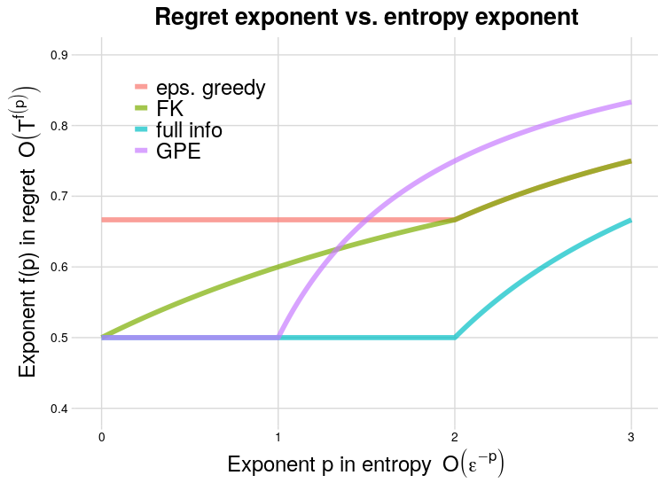
Figure 1: Exponent in regret upper bound (up to logarithmic factors) as a function of the exponent in the (supremum norm) covering entropy. FK is the theoretical upper bound of Foster and Krishnamurthy [2018]. Full info is the bound achieved by Empirical Risk Minimizers under full information feedback.

1.1 Previous work

Many contributions have been made to the area of nonparametric contextual bandits. Among others, one way to classify them is according to whether they rely on some version of the exponential weights algorithm, on optimization oracles, or on a discretization of the covariates space.

Exponential weights-based algorithms.

The exponential weights algorithm has a long history in adversarial online learning, dating back to the seminal articles of Vovk [1990] and Littlestone and Warmuth [1994]. The Exp3 algorithm of Auer et al. [2002b] is the first instance of exponential weigthts for the adversarial multi-armed bandit problem. The Exp4 algorithm of Auer et al. [2002a] extends it to the contextual bandit setting. Infinite policy classes can be handled by running a version of the Exp4 algorithm on an $\varepsilon$-cover of the policy class. While the Exp4 algorithm enjoys optimal (in a minimax sense) regret guarantees, it requires maintaining a set of weights over all elements of the cover, and is thus intractable for most nonparametric classes, because their covering numbers typically grow exponentially in $1/\epsilon$. Cesa-Bianchi et al. [2017] proposed the first cover-based efficient online learning algorithm. Their algorithm relies on a hierarchical cover obtained by the celebrated chaining device of Dudley [1967]. It achieves the minimax regret under the full information feedback model but not under the bandit feedback model, although it yields rate improvements over past works for large nonparametric policy classes. Cesa-Bianchi et al. [2017]’s regret bounds are expressed in terms of an entropy integral. An alternative approach to nonparametric adversarial online learning is that of Chatterji et al. [2019], who proposed an efficient exponential-weights algorithm for a reproducing kernel Hilbert-space (RKHS) comparison class. They characterized the regret in terms of the eigen-decay of the kernel. They obtained optimal regret if the kernel has exponential eigen-decay.

Oracle efficient algorithms.

The first oracle-based CB algorithm is the epoch-greedy algorithm of Langford and Zhang [2008]. Epoch-greedy allows to turn any supervised learning algorithm into a CB algorithm, making it practical and efficient (in terms of the number of calls to a supervised classification subroutine). Its regret can be characterized in a straighforward manner as a function of the sample complexity of the supervised learning algorithm, but is suboptimal. Dudik et al. [2011] introduced RandomizedUCB, the first regret-optimal efficient CB algorithm. Agarwal et al. [2014] improved on their work by requiring fewer calls to the oracle. [Foster et al., 2018] pointed out that the aforementioned algorithms rely on cost-sensitive classification oracles, which are in general intractable (even though for some relatively natural classes there exist efficient algorithms). Foster et al. [2018] proposed regret-optimal, regression oracles-based algorithms, motivated by the fact that regression oracles can in general be implement efficiently. Another way to make tractable these oracles is, in the case of cost-sensitive classification oracles, to use surrogate losses, as studied by Foster and Krishnamurthy [2018]. They gave regret upper bounds (see Figure 1) and a nonconstructive proof of the existence of an algorithm that achieves them. They also proposed an epoch greedy-style algorithm that achieves the best regret guarantees to date for entropy $\log N(\epsilon,\Pi)$ of order $\epsilon^{-p}$ for some $p>2$. The caveat of the surrogate loss-based approach is that guarantees are either in terms of so-called margin-based regret, or can be expressed in terms of the usual regret, but under the so-called realizability assumption. We refer the interested reader to Foster and Krishnamurthy [2018] for further details.

Covariate space discretization-based algorithms.

A third way to design nonparametric CB algorithms consists in discretizing the context space into bins and running multi-armed bandit algorithms in each bin. This approach was pioneered by Rigollet and Zeevi [2010] and extended by Perchet and Rigollet [2013]. They take a relatively different perspective from the previously mentioned works, in the sense that the comparison class is defined in an implicit fashion: they assume that the expected reward of each action is a smooth (Hölder) function of the context, and they compete against the policy defined by the argmax over actions of the expected reward. Their regret guarantees are optimal in a minimax sense.

1.2 Our contributions

Primary contribution.

In this article, we introduce the Generalized Policy Elimination algorithm, derived from the Policy Elimination algorithm of Dudik et al. [2011]. GPE is an oracle-efficient algorithm, of which the regret can be bounded in terms of the metric entropy of the policy class. In particular we show that if the entropy is integrable, then GPE has optimal regret, up to logarithmic factors. The key enabler of our results is a new maximal inequality for martingale processes (Theorem 5 in appendix B), inspired by [van de Geer, 2000, van Handel, 2011]. Although our regret upper bounds for GPE are no longer optimal for policy classes with non-integrable entropy, we show that we can use the same type of martingale process techniques to design an $\varepsilon$-greedy type algorithm that matches the current best upper bounds.

Comparison to previous work.

Earlier works on regret-optimal oracle-efficient algorithms [Dudik et al., 2011, Agarwal et al., 2014, Foster et al., 2018, for instance] have in common that the regret analysis holds for a finite number of policies or for policy classes with finite VC dimension. GPE is the first oracle-efficient algorithm for which are proven regret optimality guarantees against a truly nonparametric policy classes (that is, larger than VC).

Secondary contributions.

In addition to the nonparametric extension of policy elimination and analysis of $\varepsilon$-greedy in terms of (bracketing) entropy, we introduce several ideas that, to the best of our knowledge, have not appeared so far in the literature. In particular, we demonstrate the possibility of doing what we call direct policy optimization, that is of directly finding a maximizer $\widehat{\pi}$ of $\pi\mapsto\widehat{\mathcal{V}}(\pi)$ over $\Pi$ where $\widehat{\mathcal{V}}(\pi)$ estimates the value $\mathcal{V}(\pi)$ of policy $\pi$. As far as we know, no example has been given yet of a nonparametric class $\Pi$ for which $\widehat{\pi}$ can be efficiently computed, although some articles postulate the availability of $\widehat{\pi}$ [Luedtke and Chambaz, 2019, Athey and Wager, 2017]. Here, we exhibit several rich classes for which direct policy optimization can be efficiently implemented. Another secondary contribution is the first formal regret bounds for the $\varepsilon$-greedy algorithm, which follows from the same type of arguments as in the analysis of GPE. We were relatively surprised to see that unlike the epoch-greedy algorithm, the $\varepsilon$-greedy algorithm has not been formally analyzed yet, to the best of our knowledge. This may be due to the fact that doing so requires martingale process theory, which has only recently started to receive attention in the CB literature.

1.3 Setting

For each $m\geq 1$, denote $[m]\doteq\{1,\ldots,m\}$.

At time $t\geq 1$, the learner observes context $W_{t}\in\mathcal{W}\doteq[0,1]^{d}$, chooses an action $A_{t}\in[K]$, $K\geq 2$, and receives the outcome/reward $Y_{t}\in\{0,1\}$. We suppose that the contexts are i.i.d. and the rewards are conditionally independent given actions and contexts, with fixed conditional distributions across time points. We denote $O_{t}$ the triple $(W_{t},A_{t},Y_{t})$, and $P$ the distribution of the infinite sequence $O_{1},O_{2},\ldots,O_{t},\ldots{}$. Moreover, let $O^{\mathrm{ref}}\doteq(W^{\mathrm{ref}},A^{\mathrm{ref}},Y^{\mathrm{ref}})$ be a random variable such that $W^{\mathrm{ref}}\sim W_{1}$, $A^{\mathrm{ref}}|W^{\mathrm{ref}}\sim\operatorname{Unif}([K])$, $Y^{\mathrm{ref}}|A^{\mathrm{ref}},W^{\mathrm{ref}}\sim Y_{1}|A_{1},W_{1}$. We denote $F_{t}$ the filtration induced by $O_{1},\ldots,O_{t}$.

Generically denoted $f$ or $\pi$, a policy is a mapping from $\mathcal{W}\times[K]$ to $\mathbb{R}_{+}$ such that, for all $w\in\mathcal{W}$, $\sum_{a\in[K]}f(a,w)=1$. Thus, a policy can be viewed as mapping a context to a distribution over actions. We say the learner is carrying out policy $\pi$ at time $t$ if, for all $a\in[K]$, $w\in\mathcal{W}$, $P[A_{t}=a|W_{t}=w]=\pi(a,w)$. Owing to statistics terminology, we also call design the policy carried out at a given time point. The value $\mathcal{V}(\pi)$ of $\pi$ writes as

$$\mathcal{V}(\pi)\doteq E_{P}\left[\sum_{a\in[K]}E_{P}[Y|A=a,W]\pi(a|W)\right].$$ (1)

For any two policies $f$ and $g$, we denote

$$V(g,f)\doteq E_{P}\left[\sum_{a\in[K]}\frac{f(a|W)}{g(a|W)}\right].$$ (2)

We call $V(g,f)$ the importance sampling (IS) ratio of $f$ and $g$. The IS ratio drives the variance of IS estimators of $\mathcal{V}(f)$ had the data been collected under policy $g$.

2 Generalized Policy Elimination

Introduced by Dudik et al. [2011], the policy elimination algorithm relies on the following key fact. Let $g_{\mathrm{ref}}$ be the uniform distribution over actions used as a reference design/policy:

$$\forall(a,w)\in[K]\times\mathcal{W},\ g_{\mathrm{ref}}(a,w)\doteq K^{-1}.$$ (3)

Proposition 1.

Let $\delta>0$. For all compact and convex set $\mathcal{F}$ of policies, there exists a policy $g\in\mathcal{F}$ such that

$$\sup_{f\in\mathcal{F}}V(\delta g_{\mathrm{ref}}+(1-\delta)g,f)\leq 2K.$$ (4)

We refer to their article for a proof of this result. Proposition 1 has an important consequence for exploration. Suppose that at time $t$ we have a set of candidate policies $\mathcal{F}_{t}$, and that the designs $g_{1},...,g_{t}$ satisfy (4) with $\mathcal{F}_{t}$ substituted for $\mathcal{F}$. We can then estimate the value of candidate policies with error uniformly small over $\mathcal{F}_{t}$. This in turn has an important implication for exploitation: we can eliminate from $\mathcal{F}_{t}$ all the policies that have value below some well-chosen threshold, yielding a new policy set $\mathcal{F}_{t+1}$, and choose the next exploration policy $g_{t+1}$ in $\mathcal{F}_{t+1}$. This reasoning suggested to Dudik et al. [2011] their policy elimination algorithm: (1) initialize the set of candidate policies to the entire policy class, (2) choose an exploration policy that ensures small value estimation error uniformly over candidate policies, (3) eliminate low value policies, (4) repeat steps (2) and (3). We present formally our version of the policy algorithm as algorithm 1 below.

In this section, we show that under an entropy condition, and if we have access to a certain optimization oracle, our GPE algorithm is efficient and beats existing regret upper bounds in some nonparametric settings. Our contribution here is chiefly to extend the regret analysis of Dudik et al. [2011] to classes of functions characterized by their metric entropy in $L_{\infty}(P)$ norm. This requires us to prove a new chaining-based maximal inequality for martingale processes (Theorem 6 in appendix B). On the computational side, our algorithm relies on having access to slightly more powerful oracles than that of Dudik et al. [2011]. We present them in subsection 2.2 and give several examples where these oracles can be implemented efficiently.

We now formally state our GPE algorithm. Consider a policy class $\mathcal{F}$. For any policy $f$, any $o=(w,a,y)\in\mathcal{W}\times[K]\times\{0,1\}$, define the policy loss and its IS-weighted counterpart

$$\ell(f)(o) \doteq f(a,w)(1-y),$$ (5)

$$\ell_{\tau}(f)(o) \doteq\frac{g_{\mathrm{ref}}(a,w)}{g_{\tau}(a,w)}f(a,w)(1-y),$$ (6)

the corresponding risk $R(f)\doteq E[\ell(f)(O^{\mathrm{ref}})]=E_{P}[\ell_{\tau}(f)(O_{\tau})]$ and its empirical counterpart $\widehat{R}_{t}(f)\doteq t^{-1}\sum_{\tau=1}^{t}\ell_{\tau}(f)(O_{\tau})$.

Inputs: policy class $\mathcal{F}$, $\epsilon>0$, sequences $(\delta_{t})_{t\geq 1}$, $(x_{t})_{t\geq 1}$.

Initialize $\mathcal{F}_{1}$ as $\mathcal{F}$.

for $t\geq 1$ do

     Find $\widetilde{g}_{t}\in\mathcal{F}_{t}$ such that, for all $f\in\mathcal{F}_{t}$,

$$\frac{1}{t-1}\sum_{\tau=1}^{t-1}\frac{f(a|W_{\tau})}{(\delta_{t}g_{\mathrm{ref}}+(1-\delta_{t})\widetilde{g}_{t})(a|W_{\tau})}\leq 2K.$$ (7)

     Define $g_{t}=\delta_{t}g_{\mathrm{ref}}+(1-\delta_{t})\widetilde{g}_{t}$.

     Observe context $W_{t}$, sample action $A_{t}\sim~{}g_{t}(\cdot|W_{t})$, collect reward $Y_{t}$.

     Define $\mathcal{F}_{t+1}$ as

$$\left\{f\in\mathcal{F}_{t}:\widehat{R}_{t}(f)\leq\min_{f\in\mathcal{F}_{t}}\widehat{R}_{t}(f)+x_{t}\right\}.$$ (8)

end for

Algorithm 1 Generalized Policy Elimination

2.1 Regret analysis

Our regret analysis relies on the following assumption.

Assumption 1 (Entropy condition).

There exist $c>0$, $p>0$ such that, for all $\epsilon>0$, $\log N(\epsilon,\mathcal{F},L_{\infty}(P))\leq c\epsilon^{-p}.$

Defining $\mathcal{F}_{t+1}\subset\mathcal{F}_{t}$ as (8), the policy elimination step, consists in removing from $\mathcal{F}_{t}$ all the policies that are known to be suboptimal with high probability. The threshold $x_{t}$ thus plays the role of the width of a uniform-over-$\mathcal{F}_{t}$ confidence interval. Set $\epsilon>0$ arbitrarily. We will show that the following choice of $(\delta_{\tau})_{\tau\geq 1}$ and $(x_{\tau})_{\tau\geq 1}$ ensures that the confidence intervals hold with probability $1-6\epsilon$, uniformly both in time and over the successive $\mathcal{F}_{\tau}$’s: for all $\tau\geq 1$, $\delta_{\tau}\doteq\tau^{-(1/2\wedge 1/(2p))}$ and

$$x_{\tau}\doteq x_{\tau}(\epsilon)\doteq\sqrt{v_{\tau}(\epsilon)}\bigg{\{}\frac{c_{1}}{\tau^{\frac{1}{2}\wedge\frac{1}{2p}}}+\frac{c_{2}+c_{5}\sqrt{v_{\tau}(\epsilon)}}{\sqrt{\tau}}$$ (9)

$$\times\sqrt{\log\left(\frac{\tau(\tau+1)}{\epsilon}\right)}+\frac{1}{\tau\delta_{\tau}}\left(c_{3}+c_{7}\log\left(\frac{\tau(\tau+1)}{\epsilon}\right)\right)\bigg{\}}$$ (10)

​​​— defined in appendix C, $v_{\tau}(\epsilon)$ is a high probability upper bound on $\sup_{f\in\mathcal{F}_{\tau}}\operatorname{Var}_{P}(\ell_{\tau}(f)(O_{\tau})|F_{\tau-1})$. It is constructed as follows. It can be shown that the conditional variance of $\ell_{\tau}(f)(O_{\tau})$ given $F_{\tau-1}$ is driven by the expected IS ratio $E_{P}[\sum_{a\in[K]}f(a,W)/g_{\tau}(a,W)|F_{\tau-1}]$. Step 7 ensures that the empirical mean over past observations of the IS ratio is no greater than $2K$, uniformly over $\mathcal{F}_{\tau}$. The gap $(v_{\tau}(\epsilon)-2K)$ is a bound on the supremum over $\mathcal{F}_{\tau}$ of the deviation between empirical IS ratios and the true IS ratios.

We now state our regret theorem for algorithm 1. Let $f^{*}\doteq\mathop{\arg\min}_{f\in\mathcal{F}}$ be the optimal policy in $\mathcal{F}$.

Theorem 1 (High probability regret bound for policy elimination).

Consider algorithm 1. Suppose that Assumption 1 is met. Then, with probability at least $1-7\epsilon$, for all $t\geq 1$,

$$\sum_{\tau=1}^{t} \left(\mathcal{V}(f^{*})-Y_{\tau}\right)$$ (11)

$$\leq\sqrt{t\log\left(\frac{1}{\epsilon}\right)}+2\sum_{\tau=1}^{t}x_{\tau}(\epsilon)+\sum_{\tau=1}^{t}\delta_{\tau}$$ (12)

$$=\begin{cases}O\left(\sqrt{t}\left(\log(\frac{t}{\epsilon})\right)^{3/2}\right)&\text{ if }p\in(0,1)\\ O\left(t^{\frac{p-1/2}{p}}\left(\log(\frac{t}{\epsilon})\right)^{3/2}\right)&\text{ if }p>1\end{cases}.$$ (13)

The proof of Theorem 1, presented in appendix C, hinges on the three following facts.

1. Controlling the supremum w.r.t. $f\in\mathcal{F}_{\tau}$ of the empirical estimate of the IS ratio (see (7) in the first step of the loop in algorithm 1) allows to control the supremum w.r.t. $f$ of the true IS ratio $V(g_{\tau},f)$.

2. With the specification of $(x_{t})_{t\geq 1}$ and $(\delta_{t})_{t\geq 1}$ sketched above we can guarantee that, with probability at least $1-3\epsilon$, $f^{*}\in\mathcal{F}_{t}\subset\ldots\subset\mathcal{F}_{1}$.

3. If $f^{*}\in\mathcal{F}_{t}$ then we can prove that, with probability at least $1-5\epsilon$, for all $\tau\in[t]$,

   $$R(\widetilde{g}_{\tau})-R(f^{*})\leq 2x_{\tau}(\epsilon).$$ (14)

   This in turn yields a high probability bound on the cumulative regret of algorithm 1.

2.2 An efficient algorithm for the exploration policy search step

We show that the exploration policy search step can be performed in $O(\text{poly}(t))$ calls to two optimization oracles that we define below. The explicit algorithm and proof of the claim are presented in appendix E.

Definition 1 (Linearly Constrained Least-Squares Oracle).

We call Linearly Constrained Least-Squares Oracle (LCLSO) over $\mathcal{F}$ a routine that, for any $t\geq 1$, $q\geq 1$, vector $w\in\mathbb{R}^{Kt}$, sequence of vectors $W_{1},...,W_{t}\in\mathcal{W}$, set of vectors $u_{1},...,u_{q}\in\mathbb{R}^{Kt}$, and scalars $b_{1},...,b_{q}$, returns, if there exists one, a solution to

$$\min_{f\in\mathcal{F}}\sum_{\begin{subarray}{c}a\in[K]\\ \tau\in[t]\end{subarray}}(w(a,\tau)-f(a,W_{\tau}))^{2}\text{ subject to }$$ (15)

$$\forall m\in[q],\sum_{\begin{subarray}{c}a\in[K]\\ \tau\in[t]\end{subarray}}u_{m}(a,\tau)f(a,W_{\tau})\leq b_{\tau}.$$ (16)

Definition 2 (Linearly Constrained Cost-Sensitive Classification Oracle).

We call Linearly Constrained Cost-Sensitive Classification Oracle (LCCSCO) over $\mathcal{F}$ a routine that, for any $t\geq 1$, $q\geq 1$, vector $C\in(\mathbb{R}_{+})^{Kt}$, set of vectors $W_{1},...,W_{t}\in\mathcal{W}$, set of vectors $u_{1},...,u_{q}\in\mathbb{R}^{Kt}$, and set of scalars $b_{1},...,b_{q}\in\mathbb{R}$ returns, if there exists one, a solution to

$$\min_{f\in\mathcal{F}}\sum_{\begin{subarray}{c}a\in[K]\\ \tau\in[t]\end{subarray}}C(a,\tau)f(a,W_{\tau})\text{ subject to }$$ (17)

$$\forall m\in[q],\sum_{\begin{subarray}{c}a\in[K]\\ \tau\in[t]\end{subarray}}u_{m}(a,\tau)f(a,W_{\tau})\leq b_{\tau}.$$ (18)

The following theorem is our main result on the computational tractability of the policy search step.

Theorem 2 (Computational cost of exploration policy search).

For every $t\geq 1$, exploration policy search at time $t$ can be performed in $O((Kt)^{2}\log t)$ calls to both LCLSO and LCCSCO.

The proof of Theorem 2 builds upon the analysis of Dudik et al. [2011]. Like them, we use the famed ellipsoid algorithm as the core component. The general idea is as follows. We show that the exploration policy search step (7) boils down to finding a point $w\in\mathbb{R}^{Kt}$ that belongs to a certain convex set $\mathcal{U}$, and to identifying a $\widetilde{g}_{t}\in\mathcal{F}_{t}$ such that $\sum_{a,\tau}(f(a,W_{\tau})-w(a,\tau))^{2}\leq\Delta$ for a certain $\Delta>0$. In section E.1, we identify $\mathcal{U}$ and $\Delta$. In section E.2, we demonstrate how to find a point in $\mathcal{U}$ with the ellipsoid algorithm.

3 Finite sample guarantees for $\varepsilon$-greedy

In this section, we give regret guarantees for two variants of the $\varepsilon$-greedy algorithm competing against a policy class characterized by bracketing entropy, denoted thereon $\log N_{[\,]}$, and defined in the appendix. Corresponding to two choices of an input argument $\phi$, the two variants of algorithm 2 differ in whether they optimize w.r.t. the policy either an estimate of its value or an estimate of its hinge loss-based risk.

We formalize this as follows. We consider a class $\mathcal{F}_{0}$ of real-valued functions over $\mathcal{W}$ and derive from it two classes $\mathcal{F}^{\mathrm{Id}}$ and $\mathcal{F}^{\mathrm{hinge}}$ defined as

$$\mathcal{F}^{\mathrm{Id}}\doteq\big{\{} (a,w)\mapsto f_{a}(w):f_{1},\ldots,f_{K}\in\mathcal{F}_{0},$$ (19)

$$\forall w\in\mathcal{W},(f_{1}(w),...,f_{K}(w))\in\Delta(K)\big{\}},$$ (20)

where $\Delta(K)$ is the $K$-dimensional probability simplex, and

$$\mathcal{F}^{\mathrm{hinge}}\doteq\big{\{} (a,w)\mapsto f_{a}(w):f_{1},\ldots f_{K}\in\mathcal{F}_{0},$$ (21)

$$\forall w\in\mathcal{W},\textstyle{\sum_{a\in[K]}}f_{a}(w)=0\big{\}}.$$ (22)

Let $\phi^{\mathrm{Id}}$ be the identity mapping and $\phi^{\mathrm{hinge}}$ be the hinge mapping $x\mapsto\max(0,1+x)$, both over $\mathbb{R}$. Following exisiting terminology [Foster and Krishnamurthy, 2018, for instance], an element of $\mathcal{F}$ is called a regressor. Each regressor $f$ is mapped to a policy $\pi$ through a policy mapping, either $\widetilde{\pi}^{\mathrm{Id}}$ if $f\in\mathcal{F}^{\mathrm{Id}}$ or $\widetilde{\pi}^{\mathrm{hinge}}$ if $f\in\mathcal{F}^{\mathrm{hinge}}$ where, for all $(a,w)\in[K]\times\mathcal{W}$,

$$\widetilde{\pi}^{\mathrm{Id}}(f)(a,w) =f(a,w),$$ (23)

$$\widetilde{\pi}^{\mathrm{hinge}}(f)(a,w) =\textbf{1}\{a=\mathop{\arg\max}_{a^{\prime}\in[K]}f(a^{\prime},w)\}.$$ (24)

For $\phi$ set either to $\phi^{\mathrm{Id}}$ or $\phi^{\mathrm{hinge}}$, for any $f:[K]\times\mathcal{W}\to\mathbb{R}$, for every $o=(w,a,y)\in\mathcal{W}\times[K]\times\{0,1\}$ and each $\tau\geq 1$, define

$$\ell^{\phi}(f)(o) \doteq\phi(f(a,w))(1-y),$$ (25)

$$\ell^{\phi}_{\tau}(f) \doteq\frac{g_{\mathrm{ref}}(a,w)}{g_{\tau}(a,w)}\phi(f(a,w))(1-y),$$ (26)

the corresponding $\phi$-risk $R^{\phi}(f)\doteq E[\ell^{\phi}(f)(O^{\mathrm{ref}})]=E_{P}[\ell^{\phi}_{\tau}(f)(O_{\tau})]$ and its empirical counterpart $\widehat{R}_{t}(f)\doteq t^{-1}\sum_{\tau=1}^{t}\ell_{\tau}^{\phi}(f)(O_{\tau})$. Finally, the risk of any policy $\pi$ is defined as $R(\pi)\doteq R^{\phi}(\pi)$ with $\phi=\phi^{\mathrm{Id}}$ and the hinge-risk of any regressor $f\in\mathcal{F}^{\mathrm{hinge}}$ is defined as $R^{\mathrm{hinge}}(f)\doteq R^{\phi}(f)$ with $\phi=\phi^{\mathrm{hinge}}$.

We can now present the $\varepsilon$-greedy algorithm.

Algorithm 2 $\varepsilon$-greedy.

Input: convex surrogate $\phi$, regressor class $\mathcal{F}$, policy mapping $\widetilde{\pi}$, sequence $(\delta_{t})_{t\geq 1}$.

Initialize $\widehat{\pi}_{0}$ as $g_{\mathrm{ref}}$

for $t\geq 1$ do

     Define policy as mixture between $g_{\mathrm{ref}}$ and $\widehat{\pi}_{t-1}$:

$$g_{t}=\delta_{t}g_{\mathrm{ref}}+(1-\delta_{t})\widehat{\pi}_{t-1}$$ (27)

     Observe context $W_{t}$, sample action $A_{t}\sim g_{t}(\cdot|W_{t})$, collect reward $Y_{t}$.

     Compute optimal empirical regressor

$$\widehat{f}_{t}=\mathop{\arg\min}_{f\in\mathcal{F}}\frac{1}{t}\sum_{\tau=1}^{t}\ell_{\tau}^{\phi}(f)(O_{\tau}).$$ (28)

     Compute optimal policy estimator $\widehat{\pi}_{t}=\widetilde{\pi}(\widehat{f}_{t})$.

end for

We consider two instantiations of the algorithm: one corresponding to $(\phi^{\mathrm{Id}},\mathcal{F}^{\mathrm{Id}},\widetilde{\pi}^{\mathrm{Id}})$ and called direct policy optimization, the other corresponding to $(\phi^{\mathrm{hinge}},\mathcal{F}^{\mathrm{hinge}},\widetilde{\pi}^{\mathrm{hinge}})$ and called hinge-risk optimization.

Regret decomposition.

Denote $\pi_{\Pi}^{*}$ the optimal policy in $\Pi\doteq\widetilde{\pi}(\mathcal{F})$ and $\pi^{*}$ any optimal measurable policy. The key idea in the regret analysis of the $\varepsilon$-greedy algorithm is the following elementary decomposition (details in appendix D): $Y_{t}-R(\pi^{*})=$

$$\underbrace{Y_{t}-E_{P}[Y_{t}|F_{t-1}]}_{\text{reward noise}}+\underbrace{\delta_{t}(R(g_{\mathrm{ref}})-R(\pi^{*}))}_{\text{exploration cost}}\\ +(1-\delta_{t})\underbrace{(R(\widehat{\pi}_{t-1})-R(\pi^{*}))}_{\text{exploitation cost}}.$$ (29)

Control of the exploitation cost.

In the direct policy optimization case, we can give exploitation cost guarantees under no assumption other than an entropy condition on $\mathcal{F}$. In the hinge-risk optimization case, we need a so-called realizability assumption. Denote $\mathbb{R}^{K}_{=0}\doteq\{x\in\mathbb{R}^{K}:\sum_{a\in[K]}x_{a}=0\}$.

Assumption 2 (Hinge-realizability).

Let

$$f^{*}\doteq\mathop{\arg\min}_{f:[K]\times\mathcal{W}\rightarrow\mathbb{R}^{K}_{=0}}R^{\mathrm{hinge}}(f)$$ (30)

be the minimizer over all measurable regressors of the hinge-risk. We say that a regressor class $\mathcal{F}^{\mathrm{hinge}}$ satisfies the hinge-realizability assumption for the hinge-risk if $f^{*}\in\mathcal{F}^{\mathrm{hinge}}$.

Imported from the theory of classification calibration, Assumption 2 allows us to bound the risk of a policy $R(\widetilde{\pi}^{\mathrm{hinge}}(f))$ in terms of the hinge-risk of the regressor $f$. The proof relies on the following result:

Lemma 1 (Hinge-calibration).

Consider a regressor class $\mathcal{F}^{\mathrm{hinge}}$. Let

$$\pi^{*}\in\mathop{\arg\min}_{\pi:[K]\times\mathcal{W}\rightarrow\Delta(K)}R(\pi)$$ (31)

be an optimal measurable policy. It holds that $R(\pi^{*})=R(\widetilde{\pi}^{\mathrm{hinge}}(f^{*}))$ and, for all $f\in\mathcal{F}^{\mathrm{hinge}}$,

$$R(\widetilde{\pi}^{\mathrm{hinge}}(f))-R(\pi^{*})\leq R^{\mathrm{hinge}}(f)-R^{\mathrm{hinge}}(f^{*}).$$ (32)

We refer the reader to Bartlett et al. [2006], Ávila Pires and Szepesvári [2016] for proofs, respectively when $K=2$ and when $K\geq 2$. Under Assumption 2, Lemma 1 teaches us that we can bound the exploitation cost in terms of the excess hinge-risk $R^{\mathrm{hinge}}(f)-\min_{f^{\prime}\in\mathcal{F}^{\mathrm{hinge}}}R^{\mathrm{hinge}}(f^{\prime})$, a quantity that we can bound by standard arguments from the theory of empirical risk minimization. The fondamental building block of our exploitation cost analysis is therefore the following finite sample deviation bound for the empirical $\phi$-risk minimizer.

Theorem 3 ($\phi$-risk exponential deviation bound for the $\varepsilon$-greedy algorithm).

Let $\phi$ and $\mathcal{F}$ be either $\phi^{\mathrm{Id}}$ and $\mathcal{F}^{\mathrm{Id}}$ or $\phi^{\mathrm{hinge}}$ and $\mathcal{F}^{\mathrm{hinge}}$. Suppose that $g_{1},\ldots,g_{t}$ is a sequence of policies such that, for all $\tau\in[t]$, $g_{\tau}$ is $F_{\tau-1}$-measurable. Suppose that there exist $B,\delta>0$ such that

$$\sup_{f_{1},f_{2}\in\mathcal{F}}\sup_{a\in[K],w\in\mathcal{W}}|\phi(f_{1}(a,w))-\phi(f_{2}(a,w))|\leq B,$$ (33)

$$\min_{\tau\in[t]}g(A_{\tau},W_{\tau})\geq\delta\text{ a.s.}$$ (34)

Define $f_{\mathcal{F}}^{*}\doteq\mathop{\arg\min}_{f\in\mathcal{F}}R^{\phi}(f)$, the $\mathcal{F}$-specific optimal regressor of the $\phi$-risk, and let $\widehat{f}_{t}$ be the empirical $\phi$-risk minimizer (28). Then, for all $x>0$ and $\alpha\in(0,B)$,

$$P\bigg{[}R^{\phi}(\widehat{f}_{t})-R^{\phi}(f^{*}_{\mathcal{F}})\geq H_{t}\left(\alpha,\delta,B^{2}K/\delta,B\right)\\ +160B\sqrt{Kx/\delta t}+3B/\delta tx\bigg{]}\leq 2e^{-x},$$ (35)

with $H_{t}(\alpha,\delta,v,B)\doteq\alpha+160\sqrt{v/t}$

$$\times\int_{\alpha/2}^{B}\sqrt{\log(1+N_{[\,]}(\epsilon,\mathcal{F},L_{2}(P))}d\epsilon+\frac{3B}{\delta t}\log 2.$$ (36)

As a direct corollary, we can express rates of convergence for the $\phi$-risk in terms of the bracketing entropy rate.

Corollary 1.

Suppose that $\log(1+N_{[\,]}(\epsilon,\mathcal{F},L_{2}(P)))=O(\epsilon^{-p})$ for some $p\in(0,1)$. Then

$$R^{\phi}(\widehat{f}_{t})-R^{\phi}(f_{\mathcal{F}}^{*})=O_{P}\left((\delta t)^{-\left(\frac{1}{2}\wedge\frac{1}{p}\right)}\right).$$ (37)

Control of the regret.

The cumulative reward noise $\sum_{\tau=1}^{t}(Y_{\tau}-E_{P}[Y_{\tau}|F_{\tau-1}])$ can be bounded by the Azuma-Hoeffding inequality. From (307) and Corollary 1, $\delta_{t}$ controls the trade off between the exploration and exploitation costs. We must therefore choose a $\delta_{t}$ that minimizes the total of these two which, from the above, scales as $O(\delta_{t}+(t\delta_{t})^{-(\frac{1}{2}\wedge\frac{1}{p})})$. The optimal choice is $\delta_{t}\propto t^{-(\frac{1}{3}\wedge\frac{1}{p+1})}$. The following theorem formalizes the regret guarantees under the form of a high-probability bound.

Theorem 4 (High probability regret bound for $\varepsilon$-greedy.).

Suppose that the bracketing entropy of the regressor class $\mathcal{F}$ satisfies $\log(1+N_{[\,]}(\epsilon,\mathcal{F},L_{2}(P))=O(\epsilon^{-p})$ for some $p>0$. Set $\delta_{t}=t^{-(\frac{1}{3}\vee\frac{p}{p+1})}$ for all $t\geq 1$. Suppose that

• either $\phi=\phi^{\mathrm{Id}}$, $\mathcal{F}$ is of the form $\mathcal{F}^{\mathrm{Id}}$, $\widetilde{\pi}=\widetilde{\pi}^{\mathrm{Id}}$,

• or $\phi=\phi^{\mathrm{hinge}}$, $\mathcal{F}$ is of the form $\mathcal{F}^{\mathrm{hinge}}$, $\widetilde{\pi}=\widetilde{\pi}^{\mathrm{hinge}}$, and $\mathcal{F}$ satisfies Assumption 2.

Then, with probability $1-\epsilon$,

$$\sum_{\tau=1}^{t}(\mathcal{V}(\pi^{*})-Y_{\tau})\leq\sqrt{t\log(2/\epsilon)}\\ +t^{\frac{p}{p+1}}\sqrt{\log(2t(t+1)/\epsilon)}.$$ (38)

4 Examples of policy classes

4.1 A nonparametric additive model

We say that $a(\epsilon)=\widetilde{O}(b(\epsilon))$ if there exists $c>0$ such that $a(\epsilon)=O(b(\epsilon)\log^{c}(1/\epsilon))$. We present a policy class that has entropy $\widetilde{O}(\epsilon^{-1})$, and over which the two optimization oracles presented in Definitions 1 and 2 reduce to linear programs. Let $\mathbb{D}([0,1])$ be the set of càdlàg functions and let the variation norm $\|\cdot\|_{v}$ be given, for all $h\in\mathbb{D}([0,1])$, by

$$\|h\|_{v}\doteq\sup_{m\geq 2}\sup_{x_{1},\ldots,x_{m}}\sum_{i=1}^{m-1}|h(x_{i+1})-h(x_{i})|$$ (39)

where the right-hand side supremum is over the subdivisions of $[0,1]$, that is over $\{(x_{1},\ldots,x_{m}):0\leq x_{1}\leq\ldots\leq x_{m}\leq 1\}$. Set $C,M>0$ then introduce

$$\mathcal{H}\doteq\left\{h\in\mathbb{D}([0,1]):\|h\|_{v}\leq M\right\}$$ (40)

and the additive nonparametric additive model derived from it by setting $\mathcal{F}_{0}\doteq$

$$\big{\{}(a,w)\mapsto\sum_{l=1}^{d}\alpha_{a,l}h_{l}(w_{l}):|\alpha_{a,l}|\leq C,h_{a,l}\in\mathcal{H}\big{\}}.$$ (41)

Let $\mathcal{F}=\mathcal{F}^{\mathrm{Id}}$ derived from $\mathcal{F}_{0}$ as in (20).

The following lemma formally bounds the entropy of the policy class.

Lemma 2.

There exists $\epsilon_{0}\in(0,1)$ such that, for all $\epsilon\in(0,\epsilon_{0})$,

$$\log N_{[\,]}(\epsilon,\mathcal{F},\|\cdot\|_{\infty})\leq K\log N_{[\,]}(\epsilon,\mathcal{F}_{0},\|\cdot\|_{\infty})$$ (42)

$$\leq Kc_{0}\epsilon^{-1}\log(1/\epsilon).$$ (43)

for some $c_{0}>0$ depending on $(C,d,M)$.

We now state a result that shows that LCLSO and LCCSCO reduce to linear programs over $\mathcal{F}$. We first need to state a definition.

Definition 3 (Grid induced by a set of points).

Consider $d$ subdivisions of $[0,1]$ of the form

$$0= w_{1,1}\leq w_{1,2}\leq\ldots\leq w_{1,q_{1}}=1,$$ (44)

$$\vdots$$ (45)

$$0= w_{d,1}\leq w_{1,2}\leq\ldots\leq w_{d,q_{d}}=1.$$ (46)

The rectangular grid induced by these $d$ subdivisions is the set of points $(w_{1,i_{1}},w_{2,i_{2}},\ldots,w_{i,i_{d}})$ with $i_{1}\in[q_{1}],...,\ i_{d}\in[q_{d}]$. We call a rectangular grid any rectangular grid induced by some set of $d$ subdivisions of $[0,1]$.

Consider a set of points $w_{1},\ldots,w_{n}\in[0,1]^{d}$. A minimal grid induced by $w_{1},\ldots w_{n}$ is any rectangular grid that contains $w_{1},\ldots w_{n}$ and that is of minimal cardinality. We denote by $G(w_{1},\ldots,w_{n})$ a minimal rectangular grid induced by $w_{1},\ldots w_{n}$ chosen arbitrarily.

Lemma 3.

Let $w_{0}=\bm{0},w_{1},\ldots,w_{t}\in[0,1]^{d}$. For all $l\in[d]$, let $\widetilde{\mathcal{H}}_{l,t}\doteq\widetilde{\mathcal{H}}_{l,t}(w_{0,l},\ldots,w_{t,l})\doteq$

$$\big{\{}x\mapsto\sum_{\tau=0}^{t}\beta_{\tau}1\{x\geq w_{\tau,l}\}:\beta_{\tau}\in\mathbb{R},\sum_{\tau=0}^{t}|\beta_{\tau}|\leq M\big{\}}$$ (47)

and $\widetilde{\mathcal{F}}_{0,t}\doteq$

$$\big{\{}(a,w)\mapsto\sum_{l=1}^{d}\alpha_{a,l}\widetilde{h}_{a,l}(w_{l}):|\alpha_{a,l}|\leq B,\widetilde{h}_{a,l}\in\mathcal{H}_{l,t}\big{\}}.$$ (48)

Let $(u_{a,\tau})_{a\in[K],\tau\in[t]}$ be a vector in $\mathbb{R}^{Kt}$. Let $\widetilde{f}^{*}$ be a solution to the following optimization problem $(\mathcal{P}_{2})$:

$$\max_{\widetilde{f}\in\widetilde{\mathcal{F}}_{0,t}} \sum_{a\in[K]}\sum_{\tau=1}^{t}u_{a,\tau}\widetilde{f}(a,W_{\tau})$$ (49)

s.t. $$\forall a\in[K],\ \forall w\in\mathcal{G}(w_{0},\ldots,w_{t}),\ \widetilde{f}(a,w)\geq 0,$$ (50)

$$\forall w\in\mathcal{G}(w_{0},\ldots,w_{t}),\ \sum_{a\in[K]}\widetilde{f}(a,w)=1.$$ (51)

Then, $\widetilde{f}$ is a solution to the following optimization problem $(\mathcal{P}_{1})$:

$$\max_{f\in\mathcal{F}_{0}} \sum_{a\in[K]}\sum_{\tau=1}^{t}u_{a,\tau}f(a,W_{\tau})$$ (52)

s.t. $$\forall a\in[K],\forall w\in[0,1]^{d},f(a,w)\geq 0,$$ (53)

$$\forall w\in[0,1]^{d},\ \sum_{a\in[K]}f(a,w)=1.$$ (54)

4.2 Càdlàg policies with bounded sectional variation norm

The class of $d$-variate càdlàg functions with bounded sectional variation norm is a nonparametric function class with bracketing entropy bounded by $O(\epsilon^{-1}\log(1/\epsilon)^{2(d-1)})$, over which empirical risk minimization takes the form of a LASSO problem. It has received attention recently in the nonparametric statistics literature [van der Laan, 2016, Fang et al., 2019, Bibaut and van der Laan, 2019]. Empirical risk minimizers over this class of functions have been termed Highly Adaptive Lasso estimators by van der Laan [2016]. The experimental study of Benkeser and van der Laan [2016] suggests that Highly Adaptive Lasso estimators are competitive against supervised learning algorithms such as Gradient Boosting Machines and Random Forests.

Sectional variation norm.

For a function $f:[0,1]^{d}\rightarrow\mathbb{R}$, and a non-empty subset $s$ of $[d]$, we call the $s$-section of $f$ and denote $f_{s}$ the restriction of $f$ to $\{x\in[0,1]^{d}:\forall i\in s,x_{i}=0\}$. The sectional variation norm (svn) is defined based on the notion of Vitali variation. Defining the notion of Vitali variation in full generality requires introducing additional concepts. We thus relegate the full definition to appendix G, and present it in a particular case. The Vitali variation of an $m$-times continuously differentiable function $g:[0,1]^{m}\rightarrow\mathbb{R}$ is defined as

$$V^{(m)}(g)\doteq\int_{[0,1]^{m}}\bigg{|}\frac{\partial^{m}g}{\partial x_{1}\ldots\partial x_{m}}\bigg{|}.$$ (55)

For arbitrary real-valued càdlàg functions $g$ on $[0,1]^{m}$ (non necessarily $m$ times continuously differentiable), the Vitali variation $V^{(m)}(g)$ is defined in appendix G. The svn of a function $f:[0,1]^{d}\rightarrow\mathbb{R}$ is defined as

$$\|f\|_{v}\doteq|f(0)|+\sum_{\emptyset\neq s\subset[d]}V^{(|s|)}(f_{s}),$$ (56)

that is the sum of its absolute value at the origin and the sum of the Vitali variation of its sections. Let $\mathbb{D}([0,1]^{d})$ be the class of càdlàg functions with domain $[0,1]^{d}$ and, for some $M>0$, let

$$\mathcal{F}_{0}\doteq\left\{f\in\mathbb{D}([0,1]^{d}):\|f\|_{v}\leq M\right\}$$ (57)

be the class of càdlàg functions with svn smaller than $M$.

Entropy bound.

The following result is taken from [Bibaut and van der Laan, 2019].

Lemma 4.

Consider $\mathcal{F}_{0}$ defined in (57). Let $P$ be a probability distribution over $[0,1]^{d}$ such that $\|\cdot\|_{P,2}\leq c_{0}\|\cdot\|_{\mu,2}$, with $\mu$ the Lebesgue measure and $c_{0}>0$. Then there exist $c_{1}>0,\epsilon_{0}\in(0,1)$ such that, for all $\epsilon\in(0,\epsilon_{0})$ and all distributions $P$ over $[0,1]^{d}$,

$$\log N_{[\,]}(\epsilon,\mathcal{F}_{0},L_{2}(P))\leq c_{1}M\epsilon^{-1}\log(M/\epsilon)^{2d-1}.$$ (58)

Representation of ERM.

We show that empirical risk minimization (ERM) reduces to linear programming in both our direct policy and hinge-risk optimization settings.

Lemma 5 (Representation of the ERM in the direct policy optimization setting).

Consider a class of policies of the form $\mathcal{F}^{\mathrm{Id}}$ (20) derived from $\mathcal{F}_{0}$ (57). Let $\phi=\phi^{\mathrm{hinge}}$. Suppose we have observed $(W_{1},A_{1},Y_{1})$, …, $(W_{t},A_{t},Y_{t})$ and let $\widetilde{W}_{1},\ldots,\widetilde{W}_{m}$ be the elements of $G(W_{1},\ldots,W_{t})$.

Let $(\beta^{a}_{j})_{a\in[K],j\in[m]}$ be a solution to

$$\begin{split}\min_{\beta\in\mathbb{R}^{Km}}&\sum_{\tau=1}^{t}\sum_{a\in[K]}\bigg{\{}\frac{1\{A_{\tau}=a\}}{g_{\tau}(A_{\tau},W_{\tau})}(1-Y_{\tau})\\ &\hskip 85.35826pt\times\sum_{j=1}^{m}\beta^{a}_{j}1\{W_{\tau}\geq\widetilde{W}_{j}\}\bigg{\}}\\ \text{ s.t. }&\forall l\in[m],\ \sum_{a\in[K]}\sum_{j=1}^{m}\beta^{a}_{j}1\{\widetilde{W}_{l}\geq\widetilde{W}_{j}\}=1,\\ &\forall l\in[m],\forall a\in[K],\ \sum_{j=1}^{m}\beta^{a}_{j}1\{\widetilde{W}_{l}\geq\widetilde{W}_{j}\}\geq 0,\\ &\forall a\in[K],\ \sum_{j=1}^{m}|\beta^{a}_{j}|\leq M.\ \end{split}$$ (59)

Then $f:(a,w)\mapsto\sum_{j=1}^{m}\beta^{a}_{j}1\{w\geq\widetilde{W}_{j}\}$ is a solution to $\min_{f\in\mathcal{F}^{\mathrm{Id}}}\sum_{\tau=1}^{t}\ell^{\phi}_{\tau}(f)(O_{\tau}).$

We present a similar result for the hinge-risk setting in appendix G. It is relatively easy to prove with the same techniques that ERM over $\mathcal{F}^{\mathrm{hinge}}$ also reduces to linear programming when $\mathcal{F}_{0}$ is an RKHS.

5 Conclusion

We present the first efficient CB algorithm that is regret-optimal against policy classes with polynomial entropy. We acknowledge that our algorithm might not be practical. It inherits some of the caveats of PE: (1) the probability of the regret bound is a pre-specified parameter, (2) if the algorithm eliminates the best policy, it never recovers.

We conjecture that regret optimality could be proven for classes with non-integrable entropy. The role of integrability is purely technical and due to our proof techniques.

Appendix A Notation

Set arbitrarily $n\geq 1$ and let $\phi$ be either $\phi^{\mathrm{Id}}$ or $\phi^{\mathrm{hinge}}$. We denote by $P_{n}$ the empirical distribution $n^{-1}\sum_{i=1}^{n}\text{Dirac}(O_{i})$. For all measurable $f:[K]\times\mathcal{W}\to\mathbb{R}$, we let $\ell_{1:n}^{\phi}(f)$ be the vector-valued random function $(\ell_{1}^{\phi}(f),\ldots,\ell_{n}^{\phi}(f))$ over $[K]\times\mathcal{W}$. In order to alleviate notation, we introduce the following empirical process theory-inspired notation. For any fixed, measurable function $f:[K]\times\mathcal{W}\to\mathbb{R}$,

$$P\ell_{1:n}(f) \doteq\frac{1}{n}\sum_{i=1}^{n}E_{P}\left[\ell_{i}^{\phi}(f)(O_{i})|F_{i-1}\right],$$ (60)

$$P_{n}\ell_{1:n}(f) \doteq\frac{1}{n}\sum_{i=1}^{n}\ell_{i}^{\phi}(f)(O_{i}),$$ (61)

$$(P-P_{n})\ell_{1:n}(f) \doteq\frac{1}{n}\sum_{i=1}^{n}\left(E_{P}\left[\ell_{i}^{\phi}(f)(O_{i})|F_{i-1}\right]-\ell_{i}^{\phi}(f)(O_{i})\right).$$ (62)

For a random measurable function $f:[K]\times\mathcal{W}\to\mathbb{R}$, we let $P\ell_{1:n}(f)\doteq P\ell_{1:n}(f^{\prime})|_{f^{\prime}=f}$, and $P_{n}\ell_{1:n}(f^{\prime})|_{f^{\prime}=f}$, $(P-P_{n})\ell_{1:n}(f^{\prime})|_{f^{\prime}=f}$.

Appendix B Maximal inequalities

B.1 The basic maximal inequality for IS-weighted martingale processes

Definition 4 (Bracketing entropy, van der Vaart and Wellner [1996]).

Given two functions $l,u:\mathcal{X}\rightarrow\mathbb{R}$, the bracket $[l,u]$ is the set of all functions $f:\mathcal{X}\rightarrow\mathbb{R}$ such that, for all $x\in\mathcal{X}$, $l(x)\leq f(x)\leq u(x)$. The bracketing number $N_{[\,]}(\epsilon,\mathcal{F},L_{r}(P))$ is the number of brackets $[l,u]$ such that $\|l-u\|_{P,r}\leq\epsilon$ needed to cover $\mathcal{F}$.

The following proposition is a well-known result relating bracketing numbers and covering numbers [van der Vaart and Wellner, 1996, for instance].

Proposition 2.

For any probability distribution $P$, for all $\epsilon>0$, $N(\epsilon,\mathcal{F},L_{r}(P))\leq N_{[\,]}(2\epsilon,\mathcal{F},L_{r}(P))$ and $N(\epsilon,\mathcal{F},\|\cdot\|_{\infty})\leq N_{[\,]}(2\epsilon,\mathcal{F},\|\cdot\|_{\infty})$.

In the statement of Theorem 1, the high-probability regret bount for GPE, we used the covering numbers in uniform norm. The previous lemma allows us to carry out the analysis in terms of bracketing numbers in uniform norm.

Theorem 5 (Maximal inequality for IS-weighted martingale processes).

Consider the setting of Section 3 in the main text. Specifically, suppose that for all $i\geq 1$, $A_{i}|W_{i}\sim g_{i}(\cdot|A_{i})$ where $g_{i}$ is $F_{i-1}$-measurable. Let $n\geq 1$, and $f_{0}\in\mathcal{F}$. Suppose that

• there exists $\delta>0$ such that, for every $i\in[n]$, $g_{i}(a,w)\geq\delta$;

• there exists $B>0$ such that $\sup_{f\in\mathcal{F}}\sup_{a,w\in[K]\times\mathcal{W}}|\phi(f(a,w))-\phi(f_{0}(a,w))|\leq B$;

• there exists $v>0$ such that $\sup_{f\in\mathcal{F}}\bar{V}_{n}(\phi(f)-\phi(f_{0}))\leq v$, where, for any pair $(f,g)$ of functions $[K]\times\mathcal{W}\rightarrow\mathbb{R}_{+}$, $\bar{V}_{n}(g)\doteq n^{-1}\sum_{i=1}^{t}V(g_{i},f)$ (the definition of $V(g,f)$ is given in (2) in the main text).

Then, for all $\alpha\in[0,B]$,

$$P\left[\sup_{f\in\mathcal{F}}M_{n}(f)\geq H_{n}(\alpha,\delta,v,B)+160\sqrt{\frac{vx}{n}}+3\frac{Bx}{\delta n}\right]\leq 2e^{-x},$$ (63)

where

$$M_{n}(f)\doteq\frac{1}{n}\sum_{i=1}^{n}E\left[\ell_{i}^{\phi}(O_{i})-\ell_{i}^{\phi}(f_{0})(O_{i})|F_{i-1}\right]-\left(\ell_{i}^{\phi}(O_{i})-\ell_{i}^{\phi}(f_{0})(O_{i})\right),$$ (64)

and

$$H_{n}(\alpha,\delta,v,B)\doteq\alpha+160\sqrt{\frac{v}{n}}\int_{\alpha/2}^{B}\sqrt{\log(1+N_{[\,]}(\epsilon,\phi(\mathcal{F}),L_{2}(P)))}d\epsilon+3\frac{B}{\delta n}\log 2.$$ (65)

Proof of theorem 5.

The proof follows closely the proof of [Theorem A.4 in van Handel, 2011].

From a conditional expectation bound to a deviation bound.

Let $x>0$ and let $A$ be the event

$$A\doteq\left\{\sup_{f\in\mathcal{F}}M_{n}(f)\geq\psi(x)\right\},$$ (66)

with $\psi(x)\doteq H_{n}(\alpha,\delta,v,B)+\sqrt{vx/n}+Bx/(\delta n)$. Observe that, for any $x>0$,

$$\psi(x)\leq E^{A}_{P}\left[\sup_{f\in\mathcal{F}}\textbf{1}\{\bar{V}_{n}(f)\leq v\}(P-P_{n})\ell_{1:n}(f)\right].$$ (67)

Therefore, to prove the claim, it suffices to prove that

$$E^{A}_{P}\left[\sup_{f\in\mathcal{F}}\textbf{1}\{\bar{V}_{n}(f)\leq v\}(P-P_{n})\ell_{1:n}(f)\right]\leq\psi\left(\log\left(1+\frac{1}{P[A]}\right)\right),$$ (68)

as this would imply

$$\Psi(x)\leq\psi\left(\log\left(1+\frac{1}{P[A]}\right)\right)\leq\psi\left(\log\left(\frac{2}{P[A]}\right)\right),$$ (69)

which, as $\psi$ is increasing, implies $P[A]\leq 2e^{-x}$, which is the wished claim.

Setting up the notation.

In this proof, we will denote

$$H\doteq\left\{\phi(f)-\phi(f_{0}):f\in\mathcal{F}\right\}.$$ (70)

Observe that by assumption $\mathcal{H}$ has diameter in $\|\cdot\|_{\infty}$ norm (and thus in $L_{2}(P)$ norm) smaller than $B$. For all $j\geq 0$, let $\epsilon_{j}=B2^{-j}$, and let

$$\mathcal{B}_{j}\doteq\{(\underline{h}^{j,\rho},\overline{h}^{j,\rho}):\rho=1,\ldots,N_{j}\}$$ (71)

be an $\epsilon_{j}$-bracketing of $\mathcal{H}$ in $L_{2}(P)$ norm. Further suppose that $\mathcal{B}_{j}$ is a minimal bracketing, that is that $N_{j}=N_{[\,]}(\epsilon_{j},\mathcal{H},L_{2}(P))$. For all $j,h$, let $\rho(j,h)$ be the index of a bracket in $\mathcal{B}_{j}$ that contains $h$, that is $\rho(j,h)$ is such that

$$\underline{h}^{j,\rho(j,f)}\leq h\leq\overline{h}^{j,\rho(j,f)}.$$ (72)

For all $h\in\mathcal{H}$, $j\geq 0$, $i\in[n]$ let

$$\lambda^{j,h}\doteq\underline{h}^{j,\rho(j,h)},$$ (73)

and

$$\Delta^{j,h}_{i}\doteq(h-\lambda^{j,h})(A_{i},W_{i}).$$ (74)

Adaptive chaining.

The core idea of the proof is a so-called adaptive chaining device: for any $h$, and any $i\in[n]$, we write

$$h(A_{i},W_{i})= h(A_{i},W_{i})-\lambda^{\tau_{i}^{h},h}(A_{i},W_{i})\vee\lambda^{\tau_{i}^{h}-1,h}(A_{i},W_{i})$$ (75)

$$+\lambda^{\tau_{i}^{h},h}(A_{i},W_{i})\vee\lambda^{\tau_{i}^{h}-1,h}(A_{i},W_{i})-\lambda^{\tau_{i}^{h}-1,h}(A_{i},W_{i})$$ (76)

$$+\sum_{j=1}^{\tau_{i}^{h}-1}\lambda^{j,h}(A_{i},W_{i})\vee\lambda^{j-1,h}(A_{i},W_{i})$$ (77)

$$+\lambda^{0,h}(A_{i},W_{i}),$$ (78)

for some $\tau_{i}^{h}\geq 0$ that plays the role of the depth of the chain. We choose the depth $\tau_{i}^{h}$ so as to control the supremum norm of the links of the chain. Specifically, we let

$$\tau_{i}^{h}\doteq\min\left\{j\geq 0:\Delta^{j,h}_{i}>a_{j}\right\}\wedge J,$$ (79)

for some $J\geq 1$, and a decreasing positive sequence $a_{j}$, which we will explicitly specify later in the proof. The chaining decomposition in 169 can be rewritten as follows:

$$h(A_{i},W_{i})= \lambda^{0,h}(A_{i},W_{i})$$ (80)

$$+\sum_{j=0}^{J}\left\{h(A_{i},W_{i})-\lambda^{j,h}\vee\lambda^{j-1,h}(A_{i},W_{i})\right\}\textbf{1}\{\tau_{i}^{h}=j\}$$ (81)

$$+\sum_{j=1}^{J}\big{\{}\left(\lambda^{j,h}(A_{i},W_{i})\vee\lambda^{j-1,h}(A_{i},W_{i})-\lambda^{j-1,h}(A_{i},W_{i})\right)\textbf{1}\{\tau_{i}^{h}=j)\}$$ (82)

$$\qquad\qquad+\left(\lambda^{j,h}(A_{i},W_{i})-\lambda^{j-1,h}(A_{i},W_{i})\right)\textbf{1}\{\tau_{i}^{h}>j\}\big{\}}$$ (83)

Denote $a_{i}^{h}\doteq\lambda^{0,h}(A_{i},W_{i})$,

$$b_{i}^{j,h}\doteq\left\{h(A_{i},W_{i})-\lambda^{j,h}\vee\lambda^{j-1,h}(A_{i},W_{i})\right\}\textbf{1}\{\tau_{i}^{h}=j\},$$ (84)

and

$$c^{j,h}_{i}\doteq \left(\lambda^{j,h}(A_{i},W_{i})\vee\lambda^{j-1,h}(A_{i},W_{i})-\lambda^{j-1,h}(A_{i},W_{i})\right)\textbf{1}\{\tau_{i}^{h}=j)\}$$ (85)

$$+\left(\lambda^{j,h}(A_{i},W_{i})-\lambda^{j-1,h}(A_{i},W_{i})\right)\textbf{1}\{\tau_{i}^{h}>j\}.$$ (86)

Overloading the notation, we will denote, for every $i\in[n]$ and function $h:[K]\times\mathcal{W}\rightarrow\mathbb{R}$,

$$\ell_{i}(h)\doteq\frac{h(A_{i},W_{i})(1-Y_{i})}{g_{i}(A_{i},W_{i})}.$$ (87)

From the linearity of $\ell_{1},\ldots,\ell_{n}$, we have that

$$(P-P_{n})\ell_{1:n}(h)=A_{n}^{h}+\sum_{j=0}^{J}B_{n}^{j,h}+\sum_{j=1}^{J}C_{n}^{j,h},$$ (88)

with

$$A_{n}^{h}\doteq \frac{1}{n}\sum_{i=1}^{n}E[\ell_{i}(a_{i}^{h})|F_{i-1}]-\ell_{i}(a_{i}^{h}),$$ (89)

$$B_{n}^{j,h}\doteq \frac{1}{n}\sum_{i=1}^{n}E[\ell_{i}(b_{i}^{j,h})|F_{i-1}]-\ell_{i}(b_{i}^{j,h}),$$ (90)

$$C_{n}^{j,h}\doteq \frac{1}{n}\sum_{i=1}^{n}E[\ell_{i}(c_{i}^{j,h}|F_{i-1}]-\ell_{i}(c_{i}^{j,h}).$$ (91)

The terms $A_{n}^{h}$, $B_{n}^{j,h}$ and $C_{n}^{j,h}$ can be intepreted as follows. For any given $h$ and chain corresponding to $h$:

• $A_{n}^{h}$ represents the root, at the coarsest level, of the chain,

• if the chain goes deeper than depth $j$, $C_{n}^{j,h}$ is the link of the chain between depths $j-1$ and $j$,

• if the chain stops at depth $j$, $B_{n}^{j,h}$ is the tip of the chain.

We control each term separately.

Control of the roots.

Observe that, for all $i\in[n]$,

$$E_{P}[\ell_{i}(a_{i}^{h})^{2}|F_{i-1}]= E_{P}\left[\frac{\lambda^{0,h}(A_{i},W_{i})^{2}}{g_{i}(A_{i}|W_{i})^{2}}(1-Y_{i})^{2}|F_{i-1}\right]$$ (92)

$$\leq E_{P}\left[\sum_{a\in[K]}\frac{\left(\lambda^{0,h}(a,W_{i})-h(a,W_{i})+h(a,W_{i})\right)^{2}}{g_{i}(a,W_{i})}\bigg{|}F_{i-1}\right]$$ (93)

$$\leq 2\delta^{-1}\left\{E_{P}\left[\sum_{a\in[K]}\left(\lambda^{0,h}(a,W_{i})-h(a,W_{i})\right)^{2}\bigg{|}F_{i-1}\right]+E_{P}\left[\sum_{a\in[K]}h(a,W_{i})^{2}\bigg{|}F_{i-1}\right]\right\}$$ (94)

$$\leq 4K\delta^{-1}\epsilon_{0}^{2}.$$ (95)

In the second line we have used that $(1-Y_{i})\in[0,1]$. As $\|\lambda^{0,h}\|_{\infty}\leq B$ and $\inf_{a,w}g_{i}(a,w)\geq\delta$, we have that

$$|\ell_{i}(a_{i}^{h})|\leq B\delta^{-1}.$$ (96)

Therefore, from lemma 6,

$$E^{A}_{P}\left[\sup_{h\in\mathcal{H}}A_{n}^{h}\right]\leq 8\epsilon_{0}\sqrt{\frac{K}{\delta}\log\left(1+\frac{N_{0}}{P[A]}\right)}+\frac{8}{3}\frac{B}{\delta n}\log\left(1+\frac{N_{0}}{P[A]}\right).$$ (97)

Control of the tips.

As $\lambda_{i}^{j,h}$ is a lower bracket, $\ell_{i}(b_{i}^{j,h})\leq 0$ and thus

$$E_{P}\left[\ell_{i}(b_{i}^{j,h})|F_{i-1}\right]-\ell_{i}(b_{i}^{j,h})\leq E_{P}\left[\ell_{i}(b_{i}^{j,h})|F_{i-1}\right]$$ (98)

$$= E_{P}\left[\frac{(h(A_{i},W_{i})-\lambda^{j,h}(A_{i},W_{i})\vee\lambda^{j,h}(A_{i},W_{i})}{g_{i}(A_{i},W_{i})}(1-Y_{i})\textbf{1}\{\tau_{i}^{h}=j\}\bigg{|}F_{i-1}\right]$$ (99)

$$\leq E_{P}\left[\frac{h(A_{i},W_{i})-\lambda^{j,h}(A_{i},W_{i})\vee\lambda^{j-1,h}(A_{i},W_{i})}{g_{i}(A_{i},W_{i})}\textbf{1}\{\tau_{i}^{h}=j\}\bigg{|}F_{i-1}\right]$$ (100)

$$\leq E_{P}\left[\frac{\Delta_{i}^{j,h}\textbf{1}\{\tau_{i}^{h}=j\}}{g_{i}(A_{i},W_{i})}\bigg{|}F_{i-1}\right].$$ (101)

We treat separately the case $j<J$ and the case $j=J$. We first start with the case $j<J$. If $\tau_{i}^{h}=j$, we must then have $\Delta_{i}^{j,h}>a_{j}$, which implies that

$$E\left[\ell_{i}(b_{i}^{j,h})\big{|}F_{i-1}\right]-\ell_{i}(b_{i}^{j,f})= E_{P}\left[\frac{\Delta_{i}^{j,h}\textbf{1}\{\tau_{i}^{h}=j\}}{g_{i}(A_{i},W_{i})}\bigg{|}F_{i-1}\right]$$ (102)

$$\leq \frac{1}{a_{j}}E\left[\frac{(\Delta_{i}^{j,h})^{2}}{g_{i}(A_{i},W_{i})}\bigg{|}F_{i-1}\right]$$ (103)

$$\leq \frac{1}{a_{j}}E\left[\sum_{a\in[K]}\left(h(a,W_{i})-\lambda^{j,h}(a,W_{i})\right)^{2}\big{|}F_{i-1}\right]$$ (104)

$$\leq \frac{K\epsilon_{j}^{2}}{a_{j}}.$$ (105)

Therefore, for $j<J$,

$$E^{A}_{P}\left[\sup_{h\in\mathcal{F}}B_{n}^{j,f}\right]\leq\frac{K\epsilon_{j}^{2}}{a_{j}}.$$ (106)

Now consider the case $j=J$. We have that

$$B_{n}^{J,h}\leq \frac{1}{n}\sum_{i=1}^{n}E_{P}\left[\Delta_{i}^{J,h}\big{|}F_{i-1}\right]$$ (107)

$$= \sum_{i=1}^{n}E_{P}\left[\frac{h(A_{i},W_{i})-\lambda^{J,h}(A_{i},W_{i})}{g_{i}(A_{i},W_{i})}\bigg{|}F_{i-1}\right]$$ (108)

$$\leq \frac{1}{n}\sum_{i=1}^{n}E_{P}\left[\sum_{a\in[K]}h(a,W_{i})-\lambda^{J,h}(a,W_{i})\bigg{|}F_{i-1}\right]$$ (109)

$$\leq \frac{1}{n}\sqrt{n}\left(\sum_{i=1}^{n}E_{P}\left[\left(\sum_{a\in[K]}h(a,W_{i})-\lambda^{J,h}(a,W_{i})\right)^{2}\bigg{|}F_{i-1}\right]\right)^{1/2}$$ (110)

$$\leq \left(\frac{K}{n}\sum_{i=1}^{n}E_{P}\left[\sum_{a\in[K]}(h(a,W_{i})-\lambda^{J,h}(a,W_{i}))^{2}|F_{i-1}\right]\right)^{1/2}$$ (111)

$$\leq K\epsilon_{J}.$$ (112)

Therefore,

$$E^{A}_{P}\left[\sup_{h\in\mathcal{H}}B_{n}^{J,h}\right]\leq K\epsilon_{J}.$$ (113)

Control of the links.

Observe that $\lambda^{j,}-\lambda^{j-1,h}=\lambda^{j,h}-h+h-\lambda^{j-1,h}$. Using that $\lambda^{j,h}\leq h$ and $\lambda^{j-1,h}\leq h$ the definitions of $\Delta^{j,h}_{i}$ and $\Delta^{j-1,h}$ yield

$$-\Delta^{j,h}_{i}\leq(\lambda^{j,h}-h)(A_{i},W_{i})\textbf{1}\{\tau_{i}^{h}>j\}\leq 0,$$ (114)

and $$0\leq(h-\lambda^{j-1,h})(A_{i},W_{i})\textbf{1}\{\tau_{i}^{h}\geq j\}\leq\Delta_{i}^{j-1,h}.$$ (115)

Therefore, recalling the definition of $c^{j,h}_{i}$, we have that

$$-\Delta_{i}^{j,h}\textbf{1}\{\tau_{i}^{h}>j\}\leq c_{i}^{j,h}\leq\Delta_{i}^{j-1,h}\textbf{1}\{\tau_{i}^{h}\geq j\}.$$ (116)

Applying $\ell_{i}$ to $c_{i}^{j,h}$ amounts to multiplying it with a non-negative random variable. Therefore,

$$-\ell_{i}(\Delta_{i}^{j,h}\textbf{1}\{\tau_{i}^{h}>j\}\leq\ell_{i}(c_{i}^{j,h}\leq)\leq\ell_{i}(\Delta_{i}^{j,h}\textbf{1}\{\tau_{i}^{j,h}\geq j\}),$$ (117)

and then

$$|\ell_{i}(c_{i}^{j,f})|\leq\Delta_{i}^{j,f}\textbf{1}\{\tau_{i}^{f}>j\}\vee\Delta_{i}^{j-1,f}\textbf{1}\{\tau_{i}^{f}\geq j\}.$$ (118)

From the definition of $\tau_{i}^{j,f}$ and the fact that $(1-Y_{i})\in[0,1]$, we have that

$$|\ell_{i}(c_{i}^{j,f})|\leq a_{j}\vee a_{j-1}.$$ (119)

Besides,

$$E_{P}\left[\ell_{i}(c_{i}^{j,f})^{2}|F_{i-1}\right]\leq 2\left\{E_{P}\left[\ell_{i}(\Delta_{i}^{j,f})^{2}|F_{i-1}\right]+E_{P}\left[\ell_{i}(\Delta_{i}^{j-1,f})^{2}|F_{i-1}\right]\right\}.$$ (120)

We have that, for all $j$,

$$E_{P}\left[\ell_{i}(\Delta_{i}^{j,h})^{2}\bigg{|}F_{i-1}\right]= E_{P}\left[\frac{(f(A_{i},W_{i})-\lambda^{j,h}(A_{i},W_{i}))^{2}(1-Y_{i})^{2}}{g_{i}^{2}(A_{i},W_{i})}\bigg{|}F_{i-1}\right]$$ (121)

$$\leq E_{P}\left[\sum_{a\in[K]}\frac{(f(a,W_{i})-\lambda^{j,h}(a,W_{i}))^{2}}{g_{i}(a,W_{i})}\bigg{|}F_{i-1}\right]$$ (122)

$$\leq \delta^{-1}K\epsilon_{j}^{2}.$$ (123)

Therefore, for all $i$, $j$,

$$E_{P}\left[(\ell_{i}(c_{i}^{j,h}))^{2}|F_{i-1}\right]\leq\delta^{-1}K(\epsilon_{j-1}^{2}+\epsilon_{j}^{2}).$$ (124)

Observe that $C_{n}^{j,h}$ depends on $h$ only through $\rho(0,h)$,…,$\rho(j,h)$. Therefore, as $h$ varies over $\mathcal{H}$, $C_{n}^{j,h}$ varies over a collection of at most

$$\bar{N}_{j}\doteq\prod_{k=0}^{j}N_{k}$$ (125)

random variables. Therefore, from lemma 6,

$$E^{A}_{P}\left[\sup_{h\in\mathcal{H}}C_{n}^{j,h}\right]\leq 4\sqrt{\frac{2K(\epsilon_{j}^{2}+\epsilon_{j-1}^{2})}{\delta n}\log\left(1+\frac{\bar{N}_{j}}{P[A]}\right)}+\frac{8}{3}\frac{a_{j}\vee a_{j-1}}{\delta n}\log\left(1+\frac{\bar{N}_{j}}{P[A]}\right)$$ (126)

End of the proof.

Collecting the bounds on $E^{A}_{P}[\sup_{h\in\mathcal{H}}B_{n}^{j,h}]$, $E^{A}_{P}[\sup_{h\in\mathcal{H}}B_{n}^{j,h}]$ and $E^{A}_{P}[\sup_{h\in\mathcal{H}}C_{n}^{j,h}]$ yields

$$E^{A}_{P}\left[\sup_{h\in\mathcal{H}}(P-P_{n})\ell_{1:n}(h)\right]\leq K\epsilon_{J}+\sum_{j=0}^{J-1}\frac{K\epsilon_{j}^{2}}{a_{j}}$$ (127)

$$+8\sqrt{\frac{K}{\delta n}\log\left(1+\frac{N_{0}}{P[A]}\right)}+\frac{8}{3}\frac{B}{\delta n}\log\left(1+\frac{N_{0}}{P[A]}\right)$$ (128)

$$+\sum_{j=1}^{J}8\sqrt{\frac{K}{\delta n}\log\left(1+\frac{\bar{N}_{j}}{P[A]}\right)}$$ (129)

$$+\sum_{j=1}^{J}\frac{8}{3}\frac{a_{j-1}}{\delta n}\log\left(1+\frac{\bar{N}_{j}}{P[A]}\right).$$ (130)

Set

$$a_{j}=\epsilon_{j}\sqrt{\frac{\delta n}{K\log(1+\bar{N}_{j}/P[A])}}.$$

Replacing $a_{j}$ in the previous display yields

$$E^{A}_{P}\left[\sup_{f\in\mathcal{F}}(P-P_{n})\ell_{1:n}(f)\right]\leq K\epsilon_{J}+\frac{8}{3}\frac{B}{\delta n}\log\left(1+\frac{N_{0}}{P[A]}\right)$$ (131)

$$+20\sum_{j=0}^{J-1}\epsilon_{j}\sqrt{\frac{K}{\delta n}\log\left(1+\frac{\bar{N}_{j+1}}{P[A]}\right)}.$$ (132)

Since $(1+\bar{N}_{j}/P[A])\leq(1+1/P[A])\prod_{k=0}^{j}(1+N_{k})$, we have

$$\sum_{j=1}^{J}\epsilon_{j-1}\sqrt{\log\left(1+\frac{\bar{N}_{j}}{P[A]}\right)}\leq 2\sum_{j=0}^{J}\epsilon_{j}\sqrt{\log\left(1+\frac{1}{P[A]}\right)+\sum_{k=0}^{j}\log(1+N_{k})}$$ (133)

$$\leq 2\left(\sum_{j=0}^{J}\epsilon_{j}\right)\sqrt{\log\left(1+\frac{1}{P[A]}\right)}+2\sum_{j=0}^{J}\epsilon_{j}\sum_{k=0}^{j}\sqrt{\log(1+N_{k})}$$ (134)

We first look at the second term. We have that

$$\sum_{j=0}^{J}\epsilon_{j}\sum_{k=0}^{j}\sqrt{\log(1+N_{k})}= \sum_{k=0}^{J}\sqrt{\log(1+N_{k})}\sum_{j=k}^{J}2^{-j}$$ (135)

$$\leq 2\sum_{k=j}^{J}2^{-k}\sqrt{\log(1+N_{k})}$$ (136)

$$= 4\sum_{k=0}^{J}(\epsilon_{k}-\epsilon_{k+1})\sqrt{\log(1+N_{k})}$$ (137)

$$\leq 4\int_{\alpha/2}^{B}\sqrt{\log(1+N_{[\,]}(\epsilon,\mathcal{F},L_{2}(P)))}d\epsilon.$$ (138)

Therefore, observing that $\sum_{j=0}^{J}\epsilon_{j}\leq 2$, and gathering the previous bounds yields that

$$E^{A}_{P}\left[\sup_{h\in\mathcal{H}}(P-P_{n})\ell_{1:n}(h)\right]$$ (139)

$$\leq K\epsilon_{J}+160\sqrt{\frac{K}{\delta n}}\int_{\alpha/2}^{B}\sqrt{\log(1+N_{[\,]}(u^{2},\mathcal{F},L_{\infty}(P))}du$$ (140)

$$+\frac{8}{3}\frac{B}{\delta n}\log\left(1+N_{[\,]}(1,\mathcal{F},L_{\infty}(P))\right)$$ (141)

$$+160\sqrt{\frac{K}{\delta n}}\sqrt{\log\left(1+\frac{1}{P[A]}\right)}+\frac{8}{3}\frac{B}{\delta n}\log\left(1+\frac{1}{P[A]}\right)$$ (142)

$$\leq H_{n}(v,\delta,\alpha)+160\sqrt{\frac{v}{n}}\sqrt{\log\left(1+\frac{1}{P[A]}\right)}+3\frac{B}{\delta n}\log\left(1+\frac{1}{P[A]}\right),$$ (143)

with

$$H_{n}(v,\delta,\alpha)\doteq K\alpha+160\sqrt{\frac{K}{\delta n}}\int_{\alpha/2}^{B}\sqrt{\log(1+N_{[\,]}(u^{2},\mathcal{F},L_{\infty}(P)))}du+3\frac{B}{\delta n}\log\left(1+N_{[\,]}(1,\mathcal{F},L_{\infty}(P))\right).$$ (144)

∎

B.2 Maximal inequality for policy elimination

Theorem 6 (Maximal inequality under parameter-dependent IS ratio bound).

Let $\mathcal{F}$ be a class of functions $\mathcal{A}\times\mathcal{W}\rightarrow[0,1]$. Suppose that we are under the contextual bandit setting described earlier, and that $g_{i}$ is the $F_{i-1}$-measurable design at time point $i$. Let, for any $i\geq 1$, any $f\in\mathcal{F}$,

$$V_{i}(f)\doteq E_{P}\left[\sum_{a\in[K]}\frac{f(a|W)}{g(a|W)}\right].$$ (145)

For any $n\geq 1$, $f\in\mathcal{F}$, denote

$$\bar{V}_{n}(f)\doteq\frac{1}{n}\sum_{i=1}^{n}V_{i}(f).$$ (146)

Let $l$ be the direct policy optimization loss, and for all $i$, let $\ell_{i}$ be its importance-sampling weighted counterpart for time point $i$, that is, for all $f\in\mathcal{F}$, $o=(w,a,y)\in\mathcal{O}$,

$$l(f)(o)\doteq \sum_{a\in[K]}C(a,W)f(a,W)$$ (147)

$$\text{ and }\ell_{i}(f)(o)\doteq \frac{f(a|w)}{g_{i}(a|w)}(1-y).$$ (148)

Suppose that there exists $\delta>0$ such, that for all $a,w\in\mathcal{A}\times\mathcal{W}$ and $i\in[n]$, $g_{i}(a|w)\geq\delta$.

Then, for all $x>0$, $v>0$, $\epsilon\in[0,1]$

$$P\left[\sup_{f\in\mathcal{F}}\textbf{1}\{\bar{V}_{n}(f)\leq v\}(P-P_{n})\ell_{1:n}(f)\geq H_{n}(v,\delta,\epsilon)+37\sqrt{\frac{vx}{n}}+3\frac{x}{\delta n}\right]\leq 2e^{-x},$$ (149)

with

$$H_{n}(v,\delta,\epsilon)\doteq\sqrt{v\epsilon}+127\sqrt{\frac{v}{n}}\int_{\sqrt{\epsilon/2}}^{1}\sqrt{\log(1+N_{[\,]}(u^{2},\mathcal{F},L_{\infty}(P)))}du+\frac{3}{\delta n}\log\left(1+N_{[\,]}(1,\mathcal{F},L_{\infty}(P))\right).$$ (150)

The proof of the preceding theorem relies on the following lemma, which is a direct corollary of corollary A.8 in van Handel [2011].

Lemma 6 (Bernstein-like maximal inequality for finite sets).

Let, for any $i\in[n],j\in[N]$, $X_{i,j}$ be an $F_{i}$-measurable random variable, and let, for any $j\in[N]$, $M_{t}^{j}\doteq\sum_{i=1}^{n}X_{i,j}$. Let for all $j\in[N]$,

$$\sigma_{n,j}^{2}\doteq\frac{1}{n}\sum_{i=1}^{n}E_{P}[X_{i,j}^{2}|F_{i-1}].$$ (151)

Suppose that for all $i\in[n]$, $j\in[N]$, $|X_{i,j}|\leq b$ a.s. for some $b\geq 0$. Then, for any event $A\in\mathcal{F}$,

$$E^{A}\left[\max_{j\in[N]}\textbf{1}\{\sigma_{n,j}^{2}\leq\sigma^{2}\}M_{t}^{j}\right]\leq 4\sigma\sqrt{\log\left(1+\frac{N}{P[A]}\right)}+\frac{8}{3}b\log\left(1+\frac{N}{P[A]}\right).$$ (152)

Proof of lemma 6.

Observe that

$$\frac{2b^{2}}{n}\sum_{i=1}^{n}E\left[\phi\left(\frac{X_{i}}{b}\right)\bigg{|}F_{i-1}\right]\leq \frac{2b^{2}}{n}\sum_{i=1}^{n}\sum_{k\geq 2}\frac{b^{k-2}}{b^{k}k!}E[X_{i}^{2}|F_{i-1}]$$ (153)

$$\leq \frac{2}{n}\sum_{k\geq 2}\frac{1}{k!}\sum_{i=1}^{n}E[X_{i}^{2}|F_{i-1}]$$ (154)

$$\leq 2\phi(1)\sigma_{n,j}^{2}$$ (155)

$$\leq 2\sigma_{n,j}^{2}.$$ (156)

The conclusion follows from corollary A.8 in van Handel [2011]. ∎

Proof of theorem 6.

The proof follows closely the proof of theorem A.4 in van Handel [2011]

From a conditional expectation bound to a deviation bound.

Let $x>0$ and let $A$ be the event

$$A\doteq\left\{\sup_{f\in\mathcal{F}}\textbf{1}\{\bar{V}_{n}(f_{\leq}v\}(P-P_{n})\ell_{1:n}(f)\geq\psi(x)\right\},$$ (157)

with

$$\psi(x)=H_{n}(v,\delta,\epsilon)+37\sqrt{\frac{vx}{n}}+3\frac{x}{\delta n}$$ (158)

Observe that for any $x>0$,

$$\psi(x)\leq E^{A}_{P}\left[\sup_{f\in\mathcal{F}}\textbf{1}\{\bar{V}_{n}(f)\leq v\}(P-P_{n})\ell_{1:n}(f)\right].$$ (159)

Therefore, to prove the claim, it suffices to prove that

$$E^{A}_{P}\left[\sup_{f\in\mathcal{F}}\textbf{1}\{\bar{V}_{n}(f)\leq v\}(P-P_{n})\ell_{1:n}(f)\right]\leq\psi\left(\log\left(1+\frac{1}{P[A]}\right)\right),$$ (160)

as this would imply

$$\Psi(x)\leq\psi\left(\log\left(1+\frac{1}{P[A]}\right)\right)\leq\psi\left(\log\left(\frac{2}{P[A]}\right)\right),$$ (161)

which, as $\psi$ is increasing, implies $P[A]\leq 2e^{-x}$, which is the wished claim.

Setting up the notation.

For all $j\geq 0$, let $\epsilon_{j}=2^{-j}$, and let

$$\mathcal{B}_{j}\doteq\{(\underline{f}^{j,\rho},\overline{f}^{j,\rho}):\rho=1,\ldots,N_{j}\}$$ (162)

be an $\epsilon_{j}$-bracketing of $\mathcal{F}$ in $L_{\infty}(P)$ norm. Further suppose that $\mathcal{B}_{j}$ is a minimal bracketing, that is that $N_{j}=N_{[\,]}(\epsilon_{j},\mathcal{F},L_{\infty}(P))$. For all $j,f$, let $\rho(j,f)$ be the index of a bracket of $\mathcal{B}_{j}$ that contains $f$, that is $\rho(j,f)$ is such that

$$\underline{f}^{j,\rho(j,f)}\leq f\leq\overline{f}^{j,\rho(j,f)}.$$ (163)

For all $f\in\mathcal{F}$, $j\geq 0$, $i\in[n]$ let

$$\lambda^{j,f}\doteq\underline{f}^{j,\rho(j,f)},$$ (164)

and

$$\Delta^{j,f}_{i}\doteq(f-\lambda^{j,f})(A_{i},W_{i}).$$ (165)

Adaptive chaining.

The core idea of the proof is a so-called adaptive chaining device: for any $f$, and any $i\in[n]$, we write

$$f(A_{i},W_{i})= f(A_{i},W_{i})-\lambda^{\tau_{i}^{f},f}(A_{i},W_{i})\vee\lambda^{\tau_{i}^{f}-1,f}(A_{i},W_{i})$$ (166)

$$+\lambda^{\tau_{i}^{f},f}(A_{i},W_{i})\vee\lambda^{\tau_{i}^{f}-1,f}(A_{i},W_{i})-\lambda^{\tau_{i}^{f}-1,f}(A_{i},W_{i})$$ (167)

$$+\sum_{j=1}^{\tau_{i}^{f}-1}\lambda^{j,f}(A_{i},W_{i})\vee\lambda^{j-1,f}(A_{i},W_{i})$$ (168)

$$+\lambda^{0,f}(A_{i},W_{i}),$$ (169)

for some $\tau_{i}^{f}\geq 0$ that plays the role of the depth of the chain. We choose the depth $\tau_{i}^{f}$ so as to control the supremum norm of the links of the chain. Specifically, we let

$$\tau_{i}^{f}\doteq\min\left\{j\geq 0:\frac{\Delta^{j,f}_{i}}{g_{i}(A_{i},W_{i})}>a_{j}\right\}\wedge J,$$ (170)

for some $J\geq 1$, and a decreasing positive sequence $a_{j}$, which we will explicitly specify later in the proof. The chaining decomposition in 169 can be rewritten as follows:

$$f(A_{i},W_{i})= \lambda^{0,f}(A_{i},W_{i})$$ (171)

$$+\sum_{j=0}^{J}\left\{f(A_{i},W_{i})-\lambda^{j,f}\vee\lambda^{j-1,f}(A_{i},W_{i})\right\}\textbf{1}\{\tau_{i}^{f}=j\}$$ (172)

$$+\sum_{j=1}^{J}\big{\{}\left(\lambda^{j,f}(A_{i},W_{i})\vee\lambda^{j-1,f}(A_{i},W_{i})-\lambda^{j-1,f}(A_{i},W_{i})\right)\textbf{1}\{\tau_{i}^{f}=j)\}$$ (173)

$$\qquad\qquad+\left(\lambda^{j,f}(A_{i},W_{i})-\lambda^{j-1,f}(A_{i},W_{i})\right)\textbf{1}\{\tau_{i}^{f}>j\}\big{\}}$$ (174)

Denote $a_{i}^{f}\doteq\lambda^{0,f}(A_{i},W_{i})$,

$$b_{i}^{j,f}\doteq\left\{f(A_{i},W_{i})-\lambda^{j,f}\vee\lambda^{j-1,f}(A_{i},W_{i})\right\}\textbf{1}\{\tau_{i}^{f}=j\},$$ (175)

and

$$c^{j,f}_{i}\doteq \left(\lambda^{j,f}(A_{i},W_{i})\vee\lambda^{j-1,f}(A_{i},W_{i})-\lambda^{j-1,f}(A_{i},W_{i})\right)\textbf{1}\{\tau_{i}^{f}=j)\}$$ (176)

$$+\left(\lambda^{j,f}(A_{i},W_{i})-\lambda^{j-1,f}(A_{i},W_{i})\right)\textbf{1}\{\tau_{i}^{f}>j\}.$$ (177)

From the linearity of $\ell_{1},\ldots,\ell_{n}$, we have that

$$(P-P_{n})\ell_{1:n}(f)=A_{n}^{f}+\sum_{j=0}^{J}B_{n}^{j,f}+\sum_{j=1}^{J}C_{n}^{j,f},$$ (178)

with

$$A_{n}^{f}\doteq \frac{1}{n}\sum_{i=1}^{n}E[\ell_{i}(a_{i}^{f})|F_{i-1}]-\ell_{i}(a_{i}^{f}),$$ (179)

$$B_{n}^{j,f}\doteq \frac{1}{n}\sum_{i=1}^{n}E[\ell_{i}(b_{i}^{j,f})|F_{i-1}]-\ell_{i}(b_{i}^{j,f}),$$ (180)

$$C_{n}^{j,f}\doteq \frac{1}{n}\sum_{i=1}^{n}E[\ell_{i}(c_{i}^{j,f}|F_{i-1}]-\ell_{i}(c_{i}^{j,f}).$$ (181)

The terms $A_{n}^{f}$, $B_{n}^{j,f}$ and $C_{n}^{j,f}$ can be intepreted as follows. For any given $f$ and chain corresponding to $f$:

• $A_{n}^{f}$ represents the root, at the coarsest level, of the chain,

• if the chain goes deeper than depth $j$, $C_{n}^{j,f}$ is the link of the chain between depths $j-1$ and $j$,

• if the chain stops at depth $j$, $B_{n}^{j,f}$ is the tip of the chain.

We control each term separately.

Control of the roots.

Observe that, for all $i\in[n]$, $|\ell_{i}(a_{i}^{f})|\leq\delta^{-1}$ a.s., and that

$$E_{P}[\ell_{i}(a_{i}^{f})^{2}|F_{i-1}]= E_{P}\left[\frac{\lambda^{0,f}(A_{i},W_{i})^{2}}{g_{i}(A_{i}|W_{i})^{2}}(1-Y_{i})^{2}|F_{i-1}\right]$$ (182)

$$\leq E_{P}\left[\sum_{a\in[K]}\frac{f(a,W_{i})}{g_{i}(A_{i}|W_{i})}|F_{i-1}\right]$$ (183)

$$= V_{i}(f).$$ (184)

In the second line we have used that, $\lambda^{0,f}(A_{i},W_{i})\leq f(A_{i},W_{i})$, that $(1-Y_{i})\in[0,1]$, and that $f(a,W_{i})\in[0,1]$. Therefore, from lemma 6,

$$E^{A}_{P}\left[\sup_{f\in\mathcal{F}}\textbf{1}\{\bar{V}_{n}(f)\leq v\}A_{n}^{f}\right]\leq 4\sqrt{\frac{v}{n}\log\left(1+\frac{N_{0}}{P[A]}\right)}+\frac{8}{3\delta n}\log\left(1+\frac{N_{0}}{P[A]}\right).$$ (185)

Control of the tips.

As $\ell_{i}(b_{i}^{j,f})\leq 0$, we have that

$$E_{P}[\ell_{i}(b_{i}^{j,f})|F_{i-1}]-\ell_{i}(b_{i}^{j,f})\leq E_{P}[\ell_{i}(b_{i}^{j,f})|F_{i-1}]$$ (186)

$$= E_{P}\left[\frac{f(A_{i},W_{i})-\lambda^{j,f}(A_{i},W_{i})\vee\lambda^{j-1,f}(A_{i},W_{i})}{g_{i}(A_{i},W_{i})}(1-Y_{i})\textbf{1}\{\tau_{i}^{f}=j\}\bigg{|}F_{i-1}\right]$$ (187)

$$\leq E_{P}\left[\frac{\Delta_{i}^{j,f}}{g_{i}(A_{i},W_{i})}\textbf{1}\{\tau_{i}^{f}=j\}\bigg{|}F_{i-1}\right]$$ (188)

We treat separately the case $j<J$ and the case $j=J$. We first start with the case $j<J$. If $\tau_{i}^{f}=j$, we must then have $\Delta_{i}^{j,f}/g_{i}(A_{i},W_{i})>a_{j}$, which implies that

$$E\left[\ell_{i}(b_{i}^{j,f})\big{|}F_{i-1}\right]-\ell_{i}(b_{i}^{j,f})\leq \frac{1}{a_{j}}E\left[\frac{(\Delta_{i}^{j,f})^{2}}{g_{i}^{2}(A_{i},W_{i})}\bigg{|}F_{i-1}\right]$$ (189)

$$\leq \frac{1}{a_{j}}E\left[\sum_{a\in[K]}\frac{f(a,W_{i})}{g_{i}(a,W_{i})}(f(a,W_{i})-\lambda^{j,f}(a,W_{i}))\bigg{|}F_{i-1}\right]$$ (190)

$$\leq \frac{1}{a_{j}}V_{i}(f)\epsilon_{j}.$$ (191)

The second line above follows from the fact that $0\leq f-\lambda^{j,f}\leq f$ since $0\leq\lambda^{j,f}\leq f$. The third line above follows from the fact that $0\leq(f-\lambda^{j,f})(a,W_{i})\leq\|f-\lambda^{j,f}\|_{\infty}\leq\epsilon_{j}$. Therefore, for $j<J$,

$$E^{A}_{P}\left[\sup_{f\in\mathcal{F}}\textbf{1}\{\bar{V}_{n}(f)\leq v\}B_{n}^{j,f}\right]\leq\frac{1}{a_{j}}v\epsilon_{j}.$$ (192)

Now consider the case $j=J$. We have that

$$B_{n}^{J,f}\leq \frac{1}{n}\sum_{i=1}^{n}E_{P}\left[\frac{(f-\lambda^{J,f})(A_{i},W_{i})}{g_{i}(A_{i},W_{i})}\bigg{|}F_{i-1}\right]$$ (193)

$$\leq \frac{1}{n}\sqrt{n}\left(\sum_{i=1}^{n}E_{P}\left[\frac{(f-\lambda^{J,f})^{2}(A_{i},W_{i})}{g_{i}^{2}(A_{i},W_{i})}\bigg{|}F_{i-1}\right]\right)^{1/2}$$ (194)

$$\leq \left(\frac{1}{n}\sum_{i=1}^{n}E_{P}\left[\sum_{a\in[K]}\frac{f(a,W_{i})}{g_{i}(a|W_{i})}(f(a,W_{i})-\lambda(a,W_{i}))|F_{i-1}\right]\right)^{1/2}$$ (195)

$$\leq \left(\frac{1}{n}\sum_{i=1}^{n}V_{i}(f)\epsilon_{J}\right)^{1/2}$$ (196)

$$\leq \sqrt{v\epsilon_{J}}.$$ (197)

The second line follows from Cauchy-Schwartz and Jensen. The third line uses the same arguments as in the case $j<J$ treated before. Therefore,

$$E^{A}_{P}\left[\sup_{f\in\mathcal{F}}\textbf{1}\{\bar{V}_{n}(f)\leq v\}B_{n}^{J,f}\right]\leq\sqrt{v\epsilon_{J}}.$$ (198)

Control of the links.

Observe that $\lambda^{j,f}-\lambda^{j-1,f}=\lambda^{j,f}-f+f-\lambda^{j-1,f}$. Using that $\lambda^{j,f}\leq f$ and $\lambda^{j-1,f}\leq f$ the definitions of $\Delta^{j,f}_{i}$ and $\Delta^{j-1,f}$ yields

$$-\Delta^{j,f}_{i}\leq(\lambda^{j,f}-f)(A_{i},W_{i})\textbf{1}\{\tau_{i}^{f}>j\}\leq 0,$$ (199)

and $$0\leq(f-\lambda^{j-1,f})(A_{i},W_{i})\textbf{1}\{\tau_{i}^{f}\geq j\}\leq\Delta_{i}^{j-1,f}.$$ (200)

Therefore, recalling the definition of $c^{j,f}_{i}$, we have that

$$-\Delta_{i}^{j,f}\textbf{1}\{\tau_{i}^{f}>j\}\leq c_{i}^{j,f}\leq\Delta_{i}^{j-1,f}\textbf{1}\{\tau_{i}^{f}\geq j\}.$$ (201)

Applying $\ell_{i}$ to $c_{i}^{j,f}$ amounts to multiplying it with a non-negative random variable. Therefore,

$$-\ell_{i}(\Delta_{i}^{j,f}\textbf{1}\{\tau_{i}^{f}>j\}\leq\ell_{i}(c_{i}^{j,f}\leq)\leq\ell_{i}(\Delta_{i}^{j,f}\textbf{1}\{\tau_{i}^{j,f}\geq j\}),$$ (202)

and then

$$|\ell_{i}(c_{i}^{j,f})|\leq\Delta_{i}^{j,f}\textbf{1}\{\tau_{i}^{f}>j\}\vee\Delta_{i}^{j-1,f}\textbf{1}\{\tau_{i}^{f}\geq j\}.$$ (203)

From the definition of $\tau_{i}^{j,f}$ and the fact that $(1-Y_{i})\in[0,1]$, we have that

$$|\ell_{i}(c_{i}^{j,f})|\leq a_{j}\vee a_{j-1}.$$ (204)

Besides,

$$E_{P}\left[\ell_{i}(c_{i}^{j,f})^{2}|F_{i-1}\right]\leq 2\left\{E_{P}\left[\ell_{i}(\Delta_{i}^{j,f})^{2}|F_{i-1}\right]+E_{P}\left[\ell_{i}(\Delta_{i}^{j-1,f})^{2}|F_{i-1}\right]\right\}.$$ (205)

We have that, for all $j$,

$$E_{P}\left[(\ell_{i}(\Delta_{i}^{j,f}))^{2}|F_{i-1}\right]= E_{P}\left[\frac{(f(A_{i},W_{i})-\lambda^{j,f}(A_{i},W_{i}))^{2}}{g_{i}(A_{i}|W_{i})^{2}}(1-Y_{i})^{2}\bigg{|}F_{i-1}\right]$$ (206)

$$\leq E_{P}\left[\sum_{a\in[K]}\frac{f(a,W_{i})}{g_{i}(a|W_{i})}(f(a,W_{i})-\lambda^{j,f}(a,W_{i}))\bigg{|}F_{i-1}\right]$$ (207)

$$\leq V_{i}(f)\epsilon_{j}.$$ (208)

Therefore, for all $i$, $j$,

$$E_{P}\left[(\ell_{i}(c_{i}^{j,f}))^{2}|F_{i-1}\right]\leq V_{i}(f)(\epsilon_{j}+\epsilon_{j-1}).$$ (209)

Observe that $C_{n}^{j,f}$ depends on $f$ only through $\rho(0,f)$,…,$\rho(j,f)$. Therefore, as $f$ varies over $\mathcal{F}$, $C_{n}^{j,f}$ varies over a collection of at most

$$\bar{N}_{j}\doteq\prod_{k=0}^{j}N_{k}$$ (210)

random variables. Therefore, from lemma 6,

$$E^{A}_{P}\left[\sup_{f\in\mathcal{F}}\textbf{1}\{\bar{V}_{n}(f)\leq v\}C_{n}^{j,f}\right]\leq 4\sqrt{\frac{v(\epsilon_{j}+\epsilon_{j-1})}{n}\log\left(1+\frac{\bar{N}_{j}}{P[A]}\right)}+\frac{8}{3}\frac{a_{j}\vee a_{j-1}}{n}\log\left(1+\frac{\bar{N}_{j}}{P[A]}\right)$$ (211)

End of the proof.

Collecting the bounds on $E^{A}_{P}[\sup_{f\in\mathcal{F}}\textbf{1}\{\bar{V}_{n}(f)\leq v\}B_{n}^{j,f}]$, $E^{A}_{P}[\sup_{f\in\mathcal{F}}\textbf{1}\{\bar{V}_{n}(f)\leq v\}B_{n}^{j,f}]$ and $E^{A}_{P}[\sup_{f\in\mathcal{F}}\textbf{1}\{\bar{V}_{n}(f)\leq v\}C_{n}^{j,f}]$ yields

$$E^{A}_{P}\left[\sup_{f\in\mathcal{F}}\textbf{1}\{\bar{V}_{n}(f)\leq v\}(P-P_{n})\ell_{1:n}(f)\right]\leq \sqrt{v\epsilon_{J}}+\sum_{j=0}^{J-1}\frac{v\epsilon^{j}}{a_{j}}$$ (212)

$$+4\sqrt{\frac{v}{n}\log\left(1+\frac{N_{0}}{P[A]}\right)}+\frac{8}{3\delta n}\log\left(1+\frac{N_{0}}{P[A]}\right)$$ (213)

$$+\sum_{j=1}^{J}4\sqrt{\frac{2\epsilon_{j-1}v}{n}\log\left(1+\frac{\bar{N}_{j}}{P[A]}\right)}$$ (214)

$$+\sum_{j=1}^{J}\frac{8}{3}\frac{a_{j-1}}{n}\log\left(1+\frac{\bar{N}_{j}}{P[A]}\right).$$ (215)

Set

$$a_{j}=\frac{3}{8}\sqrt{\frac{nv\epsilon_{j}}{\log(1+\bar{N}_{j+1}/P[A])}}.$$

Replacing $a_{j}$ in the previous display yields

$$E^{A}_{P}\left[\sup_{f\in\mathcal{F}}\textbf{1}\{\bar{V}_{n}(f)\leq v\}(P-P_{n})\ell_{1:n}(f)\right]\leq \sqrt{v\epsilon_{J}}+\frac{8}{3\delta n}\log\left(1+\frac{N_{0}}{P[A]}\right)$$ (216)

$$+\sum_{j=0}^{J}(8+2\sqrt{2})\sqrt{\frac{v\epsilon_{j}}{n}\log\left(1+\frac{\bar{N}_{j}}{P[A]}\right)}.$$ (217)

Since $(1+\bar{N}_{j}/P[A])\leq(1+1/P[A])\prod_{k=0}^{j}(1+N_{k})$, we have

$$\sum_{j=0}^{J}\sqrt{\epsilon_{j}\log\left(1+\frac{\bar{N}_{j}}{P[A]}\right)}\leq \sum_{j=0}^{J}\sqrt{\epsilon_{j}}\sqrt{\log\left(1+\frac{1}{P[A]}\right)+\sum_{k=0}^{j}\log(1+N_{k})}$$ (218)

$$\leq \left(\sum_{j=0}^{J}\sqrt{\epsilon_{j}}\right)\sqrt{\log\left(1+\frac{1}{P[A]}\right)}+\sum_{j=0}^{J}\sqrt{\epsilon_{j}}\sum_{k=0}^{j}\sqrt{\log(1+N_{k})}$$ (219)

We first look at the second term. We have that

$$\sum_{j=0}^{J}\sqrt{\epsilon_{j}}\sum_{k=0}^{j}\sqrt{\log(1+N_{k})}= \sum_{k=0}^{J}\sqrt{\log(1+N_{k})}\sum_{j=k}^{J}(\sqrt{2})^{-j}$$ (220)

$$\leq \frac{\sqrt{2}}{\sqrt{2}-1}\sum_{k=0}^{J}(\sqrt{2})^{-k}\sqrt{\log(1+N_{k})}$$ (221)

$$= \left(\frac{\sqrt{2}}{\sqrt{2}-1}\right)^{2}\sum_{k=0}^{J}(\epsilon_{k}-\epsilon_{k+1})\sqrt{\log(1+N_{k})}.$$ (222)

Letting $u_{k}=\sqrt{\epsilon_{k}}$, we have that $N_{k}=N_{[\,]}(u^{2}_{k},\mathcal{F},L_{\infty}(P))$ and thus

$$\sum_{j=0}^{J}\sqrt{\epsilon_{j}}\sum_{k=0}^{j}\sqrt{\log(1+N_{k})}\leq \int_{u_{J+1}}^{u_{1}}\sqrt{\log(1+N_{[\,]}(u^{2},\mathcal{F},L_{\infty}(P)))}du.$$ (223)

Therefore, observing that $\sum_{j=0}^{J}\sqrt{\epsilon_{j}}\leq\sqrt{2}/(\sqrt{2}-1)$, and gathering the previous bounds yields that

$$E^{A}_{P}\left[\sup_{f\in\mathcal{F}}\textbf{1}\{\bar{V}_{n}(f)\leq v\}(P-P_{n})\ell_{1:n}(f)\right]$$ (224)

$$\leq \sqrt{v\epsilon_{J}}+(8+2\sqrt{2})\left(\frac{\sqrt{2}}{\sqrt{2}-1}\right)^{2}\sqrt{\frac{v}{n}}\int_{\sqrt{\epsilon_{J}/2}}^{1}\sqrt{\log(1+N_{[\,]}(u^{2},\mathcal{F},L_{\infty}(P))}du$$ (225)

$$+\frac{8}{3}\frac{1}{\delta n}\log\left(1+N_{[\,]}(1,\mathcal{F},L_{\infty}(P))\right)$$ (226)

$$+\frac{\sqrt{2}}{\sqrt{2}-1}(8+2\sqrt{2})\sqrt{\frac{v}{n}}\sqrt{\log\left(1+\frac{1}{P[A]}\right)}+\frac{8}{3\delta n}\log\left(1+\frac{1}{P[A]}\right)$$ (227)

$$\leq H_{n}(v,\delta,\epsilon_{J})+37\sqrt{\frac{v}{n}}\sqrt{\log\left(1+\frac{1}{P[A]}\right)}+\frac{3}{\delta n}\log\left(1+\frac{1}{P[A]}\right),$$ (228)

with

$$H_{n}(v,\delta,\epsilon)\doteq\sqrt{v\epsilon}+127\sqrt{\frac{v}{n}}\int_{\sqrt{\epsilon/2}}^{1}\sqrt{\log(1+N_{[\,]}(u^{2},\mathcal{F},L_{\infty}(P)))}du+\frac{3}{\delta n}\log\left(1+N_{[\,]}(1,\mathcal{F},L_{\infty}(P))\right).$$ (229)

∎

Appendix C Regret analysis of the policy evaluation algorithm

C.1 Definition of $v_{\tau}$ and constants in the definition of $x_{\tau}$

For all $\delta>0$, $v>0$, $p>0$, $\tau\geq 1$, let

$$a_{\tau}(\epsilon,\delta,v,p)\doteq\sqrt{v}\left\{\frac{c_{1}(c,p)}{\tau^{\frac{1}{2}\wedge\frac{1}{2p}}}+\frac{c_{2}}{\sqrt{\tau}}\sqrt{\log\left(\frac{\tau(\tau+1)}{\epsilon}\right)}+\frac{1}{\delta\tau}\left(c_{3}+c_{4}\log\left(\frac{\tau(\tau+1)}{\epsilon}\right)\right)\right\},$$ (230)

with

$$c_{1}(c,p)\doteq\begin{cases}\frac{127\sqrt{c}}{1-p}&\text{ if }p\in(0,1)\\ 1+\frac{127\sqrt{c}2^{\frac{p-1}{2}}}{p-1}&\text{ if }p>1,\end{cases}$$ (231)

$c_{2}=37$, $c_{3}=3\log 2$, and $c_{4}=3$. For all $\delta>0$, $v>0$, $\tau\geq 1$, let

$$b_{\tau}(\epsilon,\delta,v)\doteq c_{5}\sqrt{\frac{v}{\tau}\log\left(\frac{\tau(\tau+1)}{\epsilon}\right)}+\frac{c_{6}}{\delta\tau}\log\left(\frac{\tau(\tau+1)}{\epsilon}\right),$$ (232)

with $c_{5}=c_{6}=2$. For all $\delta>0$, $v>0$, $\tau\geq 1$, $p>0$, let

$$x_{\tau}(\epsilon,\delta,v,p)\doteq 2(a_{\tau}(\epsilon,\delta,v,p)+b_{\tau}(\epsilon,\delta,v)).$$ (233)

For all $\delta>0$, $\tau\geq 1$, let

$$v_{\tau}(\epsilon,\delta)\doteq 2K+\delta^{-1}\left\{\frac{c^{\prime}_{1}(c,p)}{\tau^{\frac{1}{2}\wedge\frac{1}{p}}}+\frac{32}{\sqrt{\tau}}\sqrt{\log\left(\frac{\tau(\tau+1)}{\epsilon}\right)}+\frac{16\log 2}{\tau}+\frac{16}{\tau}\log\left(\frac{\tau(\tau+1)}{\epsilon}\right)\right\},$$ (234)

with

$$c^{\prime}_{1}(c,p)\doteq\begin{cases}\frac{64\sqrt{c}}{1-p/2}&\text{ if }p\in(0,2),\\ 1+\frac{64\times 2^{p/2-1}\sqrt{c}}{p/2-1}&\text{ if }p>1.\end{cases}$$ (235)

The quantity $v_{\tau}$ from the main text is defined as $v_{\tau}\doteq v_{\tau}(\epsilon,\delta_{\tau})$.

We can now give the explicit definitions of the sequences $(\delta_{t})$ and $(x_{t})$. For all $\tau\geq 1$, let

$$\delta_{\tau}\doteq\tau^{-\left(\frac{1}{2}\wedge\frac{1}{2p}\right)}\qquad\text{and }\qquad x_{\tau}\doteq x_{\tau}(\epsilon,\delta_{\tau},v_{\tau}(\epsilon,\delta_{\tau}),p).$$ (236)

The constant $c_{7}$ in the main text is defined as $c_{7}\doteq c_{4}+c_{6}$.

C.2 Proofs

Lemma 7 (Bound in the max IS ratio in terms of max empirical IS ratio).

. Consider a class of policies $\mathcal{F}$ as in the current section. Suppose that $g:\mathcal{A}\times\mathcal{W}\rightarrow[0,1]$ is such that $g$ is uniformly lower bounded by some $\delta>0$, that is, for all $a,w\in\mathcal{A}\times\mathcal{W},g(a,w)\geq\delta$.

Suppose that assumption A1 holds. Then, for all $\epsilon>0$,

$$P\left[\sup_{f\in\mathcal{F}}(P-P_{n})\left\{\sum_{a\in[K]}\frac{f(a|W)}{g(a|W)}\right\}\geq v_{n}(\epsilon,\delta)-2K\right]\leq 2\frac{\epsilon}{n(n+1)}.$$ (237)

The proof of lemma 7 relies on the following result, which is a slighlty modified version of corollary 6.9 in Massart [2007]. The only differences are that

• we state it with lower bound of the entropy integral $\alpha/2>0$, instead of $0$, which makes appear an approximation error term $\alpha$,

• we state it for i.i.d. random variables instead of independent random variables, we set to 1 the value of $\epsilon$ in the original statement of the theorem.

Proposition 3.

Let $\mathcal{F}$ be a class of functions $f:\mathcal{X}\rightarrow\mathbb{R}$. Let $X_{1},\ldots,X_{n}$ be i.i.d. random variables with domain $\mathcal{X}$ and common marginal distribution $P$. Suppose that there exists $\sigma$ and $b$ such that, for all $f\in\mathcal{F}$, for any $k\geq 2$,

$$E_{P}[|f(X)|^{k}]\leq\frac{k!}{2}\sigma^{2}b^{k-2}.$$ (238)

Assume that for all $\epsilon>0$, there exists a set of brackets $\mathcal{B}(\epsilon,b)$ covering $\mathcal{F}$ such that, for all bracket $[l,u]$ in $\mathcal{B}(\epsilon,\delta)$,

$$E[((u-l)(X))^{k}]\leq\frac{k!}{2}\epsilon^{2}b^{k-2}.$$ (239)

We call such a $\mathcal{B}(\epsilon,\delta)$ an $(\epsilon,b)$ bracketing of $\mathcal{F}$, and we denote $\mathcal{N}_{[\,]}(\epsilon,b\,\mathcal{F})$ the minimal cardinality of such an $\mathcal{B}(\epsilon,b)$.

Then, for all $\alpha\in(0,\sigma)$, and for all $x>0$,

$$P\left[\sup_{\in\mathcal{F}}(P-P_{n})f\geq H_{n}(\alpha,\sigma,b)+10\sigma\sqrt{\frac{x}{n}}+2bx\right]\leq e^{-x},$$ (240)

where

$$H_{n}(\alpha,\sigma,b)\doteq\alpha+\frac{27}{\sqrt{n}}\int_{\alpha/2}^{\sigma}\sqrt{\log\mathcal{N}_{[\,]}(\epsilon,b,\mathcal{F})}d\epsilon+\frac{2(\sigma+b)}{n}\log\mathcal{N}_{[\,]}(\sigma,b,\mathcal{F}).$$ (241)

Proof of proposition 3.

It suffices to choose $J$ in the proof of corollary 6.9 in Massart [2007] such that $\alpha/2\leq\epsilon_{J}<\alpha$, and not let it go to $\infty$ at the end of the proof. ∎

Proof of lemma 7.

Let

$$\mathcal{H}\doteq\left\{h:w\mapsto\sum_{a\in[K]}\frac{f(a,w)}{g(a,w)}:f\in\mathcal{F}\right\}.$$ (242)

Observe that, for all $h\in\mathcal{H}$, $h(W)|\leq\delta^{-1}$, as $g\geq\delta$, and thus $E_{P}[h^{2}(W)]\leq\delta^{-2}$. Observe that an $\epsilon$-bracketing of $\mathcal{F}$ in $L_{2}(P)$ induces a $(\sqrt{K}\epsilon\delta^{-1},b)$ bracketing of $\mathcal{H}$ in the sense of proposition 3. Therefore, from proposition 3

$$P\left[\sup_{f\in\mathcal{F}}(P-P_{n})f\geq v_{n}(\epsilon,\delta)-2K\right]\leq\frac{\epsilon}{n(n+1)}.$$ (243)

∎

The following lemma shows that, with high probability, the policy elimination algorithm doesn’t eliminate the optimal policy.

Lemma 8.

Suppose that A1 holds. Suppose $(x_{t}(\epsilon))$ is as specified in subsection 2.1. Then, for all $t\geq 1$,

$$P[f^{*}\in\mathcal{F}]\geq 1-3\epsilon.$$ (244)

Proof.

Denote $\hat{f}_{\tau}\doteq\arg\min_{f\in\mathcal{F}_{\tau}}\hat{R}_{\tau}(f)$. We have that

$$\hat{R}_{\tau}(f^{*})-\hat{R}_{\tau}(\hat{f}_{\tau})\leq R(f^{*})-R(\hat{f}_{\tau})$$ (245)

$$+\hat{R}_{\tau}(f^{*})-R(f^{*})$$ (246)

$$+R(\hat{f}_{\tau})-\hat{R}_{\tau}(\hat{f}_{\tau})$$ (247)

$$\leq \hat{R}_{\tau}(f^{*})-R(f^{*})$$ (248)

$$+\sup_{f\in\mathcal{F}_{\tau}}R(f)-\hat{R}_{\tau}(f).$$ (249)

Define the event

$$\mathcal{E}_{1,t}\doteq\left\{\forall\tau\in[t]:\sup_{f\in\mathcal{F}_{\tau}}V(g_{\tau},f)\leq v_{\tau}(\epsilon,\delta_{\tau})\right\},$$ (250)

where $v_{\tau}(\epsilon,\delta_{\tau})$ is defined in subsection 2.1. From lemma 7,

$$P[\mathcal{E}_{1,t}]\geq 1-2\epsilon.$$ (251)

For all $\tau\in[t]$, define the event

$$\mathcal{E}_{2,t}\doteq\left\{\max_{\tau\in[t]}\sup_{f\in\mathcal{F}_{\tau}}R(f)-\hat{R}_{\tau}(f)\leq a_{\tau}(\epsilon,\delta_{\tau},v_{\tau}(\epsilon,\delta_{\tau}),p)\right\},$$ (252)

where $a_{\tau}$ is defined in subsection 2.1. From theorem 6,

$$P[\mathcal{E}_{2,t}^{c},\mathcal{E}_{1,t}]\leq\epsilon.$$ (253)

We now turn to controlling $\hat{R}_{\tau}(f^{*})-R(f^{*})$. So as to be able to obtain a high probability bound scaling as $\sqrt{v_{\tau}(\epsilon,\delta_{\tau})/\tau}$, we need $f^{*}$ to be in $\mathcal{F}_{\tau}$. As we are about to show, if the desired bound holds, that $\mathcal{E}_{1,t}\cap\mathcal{E}_{2,t}$ holds, and that $f^{*}\in\mathcal{F}_{\tau}$, them we will have that $f^{*}\in\mathcal{F}_{\tau+1}$. This motivates a reasoning by induction.

Let, for all $\tau\in[t]$,

$$\mathcal{E}_{3,\tau}\doteq\left\{\hat{R}_{\tau}(f^{*})-R(f^{*})\leq b_{\tau}(\epsilon,\delta_{\tau},v(\epsilon,\delta_{\tau}))\right\},$$ (254)

where $b_{\tau}$ is defined in subsection 2.1. We are going to show by induction that for all $\tau\in[t]$,

$$P\left[\mathcal{E}_{3,t}^{c},\mathcal{E}_{1,t},\mathcal{E}_{2,t}\right]\leq\sum_{s=1}^{\tau}\frac{\epsilon}{s(s+1)}.$$ (255)

By convention, we let $\mathcal{E}_{3,0}\doteq\{f^{*}\in\mathcal{F}\}$. and $\sum_{s=1}^{0}1/(s(s+1))=0$. The induction claim thus trivially holds at $\tau=0$. Consider $\tau\in[t]$. Suppose that

$$P[\mathcal{E}_{3,\tau-1}^{c},\mathcal{E}_{1,t},\mathcal{E}_{2,t}]\leq\sum_{s=1}^{\tau-1}\frac{\epsilon}{s(s+1)}.$$ (256)

Observe that $\mathcal{E}_{\tau-1}\cap\mathcal{E}_{1,t}\cap\mathcal{E}_{2,t}$ implies $f^{*}\in\mathcal{F}_{\tau}$ as we then have

$$\hat{R}_{\tau}(f^{*})-\hat{R}_{\tau}(\hat{f}_{\tau})\leq a_{\tau-1}(\epsilon,\delta_{\tau-1},v_{\tau-1}(\epsilon,\delta_{\tau-1}),p)+b_{\tau-1}(\epsilon,\delta_{\tau-1},v_{\tau-1}(\epsilon,\delta_{\tau-1}))$$ (257)

$$< x_{\tau-1}(\epsilon,\delta_{\tau-1},v_{\tau-1}(\epsilon,\delta_{\tau-1})).$$ (258)

Using this fact, distinguishing the cases $\mathcal{E}_{3,\tau-1}$ and $\mathcal{E}_{3,\tau-1}^{c}$, and using the induction hypothesis yields

$$P[\mathcal{E}_{3,\tau}^{c},\mathcal{E}_{1,t},\mathcal{E}_{2,t}]\leq P[\mathcal{E}_{3,\tau}^{c},\mathcal{E}_{3,\tau-1},\mathcal{E}_{1,t},\mathcal{E}_{2,t}]+P[\mathcal{E}_{3,\tau-1}^{c},\mathcal{E}_{1,t},\mathcal{E}_{2,t}]$$ (259)

$$\leq P[\mathcal{E}_{3,\tau}^{c},f^{*}\in\mathcal{F},\mathcal{E}_{2,t}]+\sum_{s=1}^{\tau-1}\frac{\epsilon}{s(s+1)}.$$ (260)

Observe that under $\{f^{*}\in\mathcal{F}_{\tau}\}\cap\mathcal{E}_{2,t}$, we have that $V(g_{\tau},f^{*})\leq v_{\tau}(\epsilon,\delta_{\tau})$ and thus

$$E[(\ell_{\tau}(f^{*})(O_{\tau}))^{2}|F_{\tau-1}]\leq Kv_{\tau}(\epsilon,\delta_{\tau}).$$ (261)

Besides, $|\ell_{\tau}(f^{*})(O_{\tau})-E[\ell_{\tau}(f^{*})(O_{\tau})|F_{\tau-1}]\leq\delta_{\tau}^{-1}$. Therefore, from Bernstein’s inequality for martingales

$$P[\mathcal{E}_{3,\tau}^{c},f^{*}\in\mathcal{F},\mathcal{E}_{2,t}]\leq\frac{\epsilon}{\tau(\tau+1)}.$$ (262)

Therefore,

$$P[\mathcal{E}^{c}_{3,\tau},\mathcal{E}_{1,t},\mathcal{E}_{2,t}]\leq\sum_{s=1}^{\tau}\frac{\epsilon}{s(s+1)}.$$ (263)

We have thus shown that, for all $\tau\in[t]$,

$$P[\mathcal{E}^{c}_{3,\tau},\mathcal{E}_{1,t},\mathcal{E}_{2,t}]\leq\sum_{s=1}^{\tau}\frac{\epsilon}{s(s+1)}.$$ (264)

Therefore,

$$P[\mathcal{E}_{3,t},\mathcal{E}_{1,t},\mathcal{E}_{2,t}]= P[\mathcal{E}_{1,t},\mathcal{E}_{2,t}]-P[\mathcal{E}^{c}_{3,t},\mathcal{E}_{1,t},\mathcal{E}_{2,t}]$$ (265)

$$= P[\mathcal{E}_{1,t}]-P[\mathcal{E}_{1,t},\mathcal{E}^{c}_{2,t}]-P[\mathcal{E}^{c}_{3,t},\mathcal{E}_{1,t},\mathcal{E}_{2,t}]$$ (266)

$$= 1-P[\mathcal{E}^{c}_{1,t}]-P[\mathcal{E}_{1,t},\mathcal{E}^{c}_{2,t}]-P[\mathcal{E}_{1,t},\mathcal{E}_{2,t},\mathcal{E}_{3,t}^{c}]$$ (267)

$$\geq 1-4\epsilon.$$ (268)

∎

The following lemma gives a bound on $\sup_{f\in\mathcal{F}_{\tau}}R(f)-R(f^{*})$ which holds uniformly in time with high probability.

Lemma 9.

Consider algorithm 1. Make assumption A1. Then, with probability $1-4\epsilon$, we have that, for all $\tau\in[t]$,

$$\sup_{f\in\mathcal{F}_{\tau}}R(f)-R(f^{*})\leq 2x_{\tau}.$$ (269)

Proof.

Observe that, for all $f\in\mathcal{F}$,

$$R(f)-R(f^{*})= \hat{R}_{\tau}(f)-\hat{R}_{\tau}(f^{*})$$ (270)

$$+R(f)-\hat{R}_{\tau}(f)$$ (271)

$$-R(f^{*})-\hat{R}_{\tau}(f^{*}))$$ (272)

$$\leq \hat{R}_{\tau}(f)-\hat{R}_{\tau}(\hat{f}_{\tau})$$ (273)

$$+\sup_{f\in\mathcal{F}_{\tau}}(R(f)-\hat{R}_{t}(f))$$ (274)

$$-(R(f^{*})-\hat{R}_{t}(f^{*}))$$ (275)

$$\leq x_{\tau}$$ (276)

$$+\sup_{f\in\mathcal{F}_{\tau}}(R(f)-\hat{R}_{t}(f))$$ (277)

$$-(R(f^{*})-\hat{R}_{t}(f^{*})).$$ (278)

Define the events

$$\mathcal{E}_{1,t}\doteq \left\{\forall\tau\in[t],\sup_{f\in\mathcal{F}_{\tau}}V(g_{\tau},f)\leq v_{\tau}(\epsilon,\delta_{\tau})\right\},$$ (279)

$$\mathcal{E}_{2,t}\doteq \left\{f^{*}\in\mathcal{F}_{t}\right\}.$$ (280)

From lemma 8,

$$P[\mathcal{E}_{1,t}]\geq 1-4\epsilon.$$ (281)

Under $\mathcal{E}_{1,t}$, we have that, for all $f\in\mathcal{F}_{\tau}$,

$$E\left[(\ell_{\tau}(f)(O_{\tau}))^{2}|F_{\tau-1}\right]\leq Kv_{\tau}(\epsilon,\delta_{\tau}).$$ (282)

Therefore, using also that $|\ell_{\tau}(f)(O_{\tau})|\leq\delta_{\tau}^{-1}$, theorem 6 gives us that, for all $\tau\in[t]$,

$$P\left[\sup_{f\in\mathcal{F}_{\tau}}R(f)-\hat{R}_{\tau}(f)\geq a_{\tau}(\epsilon,v_{\tau}(\epsilon,\delta_{\tau}),\delta_{\tau},p),\mathcal{E}_{1,t}\right]\leq\frac{\epsilon}{\tau(\tau+1)},$$ (283)

which, by a union bound gives us that

$$P\left[\mathcal{E}_{3,t}^{c},\mathcal{E}_{1,t}\right]\leq\epsilon,$$ (284)

with

$$\mathcal{E}_{3,t}\doteq\left\{\forall\tau\in[t],\sup_{f\in\mathcal{F}_{\tau}}R(f)-\hat{R}_{\tau}(f)\leq a_{\tau}(\epsilon,v_{\tau}(\epsilon,\delta_{\tau}),\delta_{\tau},p)\right\}.$$ (285)

We now consider the term $\hat{R}_{\tau}(f)-R(f^{*})$. We have that

$$\hat{R}_{\tau}(f^{*})-R(f^{*})=\frac{1}{t}\sum_{\tau=1}^{t}\ell_{\tau}(f^{*})(O_{\tau})-E[\ell_{\tau}(f^{*})(O_{\tau})|F_{\tau-1}]$$ (286)

Under $\mathcal{E}_{1,t}\cap\mathcal{E}_{2,t}$, each term in the sum satisfies

$$E_{P}\left[(\ell_{\tau}(f^{*})(O_{\tau}))^{2}|F_{\tau-1}\right]\leq Kv_{\tau}(\epsilon,\delta_{\tau})$$ (287)

and

$$|\ell_{\tau}(f^{*})(O_{\tau})-E_{P}\left[\ell_{\tau}(f^{*})(O_{\tau})|F_{\tau-1}\right]\leq\delta_{\tau}^{-1}.$$ (288)

Therefore, from Bernstein’s inequality and a union bound, letting

$$\mathcal{E}_{4,t}\doteq\left\{\forall\tau\in[t],\hat{R}_{\tau}(f^{*})-R(f^{*})\leq b_{\tau}(\delta,v_{\tau}(\epsilon,\delta_{\tau}),\delta_{\tau})\right\},$$ (289)

we have that

$$P[\mathcal{E}_{4,t}^{c},\mathcal{E}_{1,t},\mathcal{E}_{2,t}]\leq\epsilon.$$ (290)

Observe that under $\mathcal{E}_{3,t}\cap\mathcal{E}_{4,t}$ it holds that

$$\forall\tau\in[t]\sup_{f\in\mathcal{F}_{\tau}}R(f)-R(f^{*})\leq x_{\tau}.$$ (291)

Therefore, to conclude the proof, it suffices to bound $P[\mathcal{E}_{3,t},\mathcal{E}_{4,t}]$. We have that

$$P[(\mathcal{E}_{3,t}\cap\mathcal{E}_{4,t})^{c}]\leq P[\mathcal{E}_{1,t},\mathcal{E}_{2,t},(\mathcal{E}_{3,t}\cap\mathcal{E}_{4,t})^{c}]+P[\mathcal{E}_{1,t}^{c}]+P[\mathcal{E}_{2,t}^{c}]$$ (292)

$$\leq P[\mathcal{E}_{1,t},\mathcal{E}_{2,t},\mathcal{E}_{3,t}^{c}]$$ (293)

$$+P[\mathcal{E}_{1,t},\mathcal{E}_{2,t},\mathcal{E}_{4,t}^{c}]+P[\mathcal{E}_{1,t}^{c}]+P[\mathcal{E}_{2,t}^{c}]$$ (294)

$$\leq 6\epsilon,$$ (295)

which yields the wished claim. ∎

We can now prove theorem 1.

Proof of theorem 1.

Observe that

$$\sum_{\tau=1}^{t}\mathcal{V}(f^{*})-Y_{\tau}= \sum_{\tau=1}^{t}(1-Y_{\tau})-E_{P}[(1-Y_{\tau})|F_{\tau-1}]$$ (296)

$$+\sum_{\tau=1}^{t}E_{P}[(1-Y_{\tau})|F_{\tau-1}]-R(f^{*}).$$ (297)

Since $(1-Y_{\tau})\in[0,1]$, from Azuma-Hoeffding, we have that, with probability at least $1-\epsilon$,

$$\sum_{\tau=1}^{t}(1-Y_{\tau})-E_{P}[(1-Y_{\tau})|F_{\tau-1}]\leq\sqrt{t\log\left(\frac{1}{\epsilon}\right)}.$$ (298)

Observe that

$$E_{P}\left[(1-Y_{\tau})|F_{\tau-1}\right]=R(g_{\tau})=\delta_{\tau}R(g_{ref})+(1-\delta_{\tau})R(\tilde{g}_{\tau}),$$ (299)

where $\tilde{g}_{\tau}\in\mathcal{F}_{\tau}$. Therefore,

$$E_{P}\left[(1-Y_{\tau})|F_{\tau-1}\right]-R(f^{*})\leq \delta_{\tau}(R(g_{ref})-R(f^{*}))+(1-\delta_{\tau})(R(\tilde{g}_{\tau})-R(f^{*}))$$ (300)

$$\leq \delta_{\tau}+(R(\tilde{g}_{\tau})-R(f^{*}))$$ (301)

From lemma 9, with probability $1-6\epsilon$, for all $\tau\in[t]$,

$$R(\tilde{g}_{\tau})-R(f^{*})\leq x_{\tau}.$$ (302)

Therefore, with probability at least $1-7\epsilon$, we have the wished bound. ∎

Appendix D Regret analysis of the $\varepsilon$-greedy algorithm

D.1 Regret decomposition

Using in particular the linearity of $\pi\mapsto R(\pi)$ and the definition of $g_{t}$, we have that

$$Y_{t}-R(\pi^{*})$$ (303)

$$= Y_{t}-E[Y_{t}|F_{t-1}]+E[Y_{t}|F_{t-1}]-R(\pi^{*})$$ (304)

$$= Y_{t}-E[Y_{t}|F_{t-1}]+R(g_{t})-R(\pi^{*})$$ (305)

$$= \underbrace{Y_{t}-E[Y_{t}|F_{t-1}]}_{\text{reward noise}}+\underbrace{\delta_{t}(R(g_{ref})-R(\pi^{*}))}_{\text{exploration cost}}$$ (306)

$$+(1-\delta_{t})\underbrace{(R(\hat{\pi}_{t-1})-R(\pi^{*}))}_{\text{exploitation cost}}.$$ (307)

D.2 Proof of deviations inequalities

Proof of theorem 3.

Observe that

$$R^{\phi}(\hat{f}_{t})-R^{\phi}(f^{*}_{\mathcal{F}})= \frac{1}{t}\sum_{\tau=1}^{t}E\left[\ell_{\tau}(f)(O_{\tau})-\ell_{\tau}(f^{*}_{\mathcal{F}})(O_{\tau})|F_{\tau-1}\right]\big{|}_{f=\hat{f}_{t}}$$ (308)

$$= \frac{1}{t}\sum_{\tau=1}^{t}\ell_{\tau}^{\phi}(\hat{f}_{t})(O_{\tau})-\ell^{\phi}_{\tau}(f^{*}_{\mathcal{F}})(O_{\tau})$$ (309)

$$+M_{t}(\hat{f}_{t})$$ (310)

with $M_{t}(f)$ as defined in (64) and where we take $f_{0}=f^{*}_{\mathcal{F}}$ in the definition of $M_{t}$. Since $\hat{f}_{t}$ is the empirical $\phi$-risk minimizer, line 309 is non-positive, and thus

$$R^{\phi}(\hat{f}_{t})-R^{\phi}(f^{*}_{\mathcal{F}})\leq M_{t}(\hat{f}_{t}).$$ (311)

Observe that, for all $f\in\mathcal{F}$,

$$|\ell^{\phi}_{\tau}(f)-\ell^{\phi}_{\tau}(f^{*}_{\mathcal{F}})|\leq\frac{B}{\delta}$$ (312)

and

$$E_{P}\left[\left((\ell_{\tau}^{\phi}(f)(O_{\tau})-\ell^{\phi}_{\tau}(f^{*}_{\mathcal{F}})(O_{\tau})\right)^{2}\big{|}F_{\tau-1}\right]= E_{P}\left[\frac{\left(\phi(f(A_{\tau},W_{\tau})-\phi(f^{*}_{\mathcal{F}}(A_{\tau},W_{\tau})\right)^{2}}{g_{\tau}(A_{\tau},W_{\tau})^{2}}(1-Y_{\tau})^{2}\big{|}F_{\tau-1}\right]$$ (313)

$$\leq E\left[\sum_{a\in[K]}\frac{\left(\phi(f(a,W_{\tau})-\phi(f^{*}_{\mathcal{F}}(a,W_{\tau})\right)^{2}}{g_{\tau}(a,W_{\tau})}\big{|}F_{\tau-1}\right]$$ (314)

$$\leq \frac{KB^{2}}{\delta}.$$ (315)

Therefore, using (311) and theorem 5, we have that

$$P\left[R^{\phi}(\hat{f}_{t})-R^{\phi}(f^{*}_{\mathcal{F}})\geq H_{t}\left(\alpha,\delta,B\sqrt{\frac{K}{\delta}},B\right)+160B\sqrt{\frac{Kx}{\delta t}}+3\frac{Bx}{\delta t}\right]\leq 2e^{-x},$$ (316)

with

$$H_{t}(\alpha,\delta,v,B)=\alpha+160\sqrt{\frac{v}{t}}\int_{\alpha/2}^{B}\sqrt{\log(1+N_{[\,]}(\epsilon,\mathcal{F},L_{2}(P)))}d\epsilon+3\frac{B}{\delta t}\log 2.$$ (317)

∎

Proof of theorem 4.

For any $p\in(0,2)\cup(2,\infty)$,

$$\int_{\alpha/2}^{B}\sqrt{\log(1+N_{[\,]}(\epsilon,\mathcal{F},L_{2}(P)}\leq\frac{\sqrt{c_{0}}}{1-p/2}\left(B^{1-p/2}-\left(\frac{\alpha}{2}\right)^{1-p/2}\right).$$ (318)

We set

$$\alpha=\begin{cases}0&\text{ for }p\in(0,2)\\ B^{2/p}\left(\frac{K}{\delta\tau}\right)^{\frac{1}{p}}&\text{ for }p>2.\end{cases}$$ (319)

Then, we have

$$H_{\tau}(\alpha,\delta,v,B)\leq\begin{cases}B\sqrt{\frac{K}{\delta\tau}}\frac{\sqrt{c_{0}}}{1-p/2}B^{1-p/2}+\frac{3B\log 2}{\delta\tau}&\text{ for }p\in(0,2),\\ B^{2/p}\left(\frac{K}{\delta\tau}\right)^{1/p}\left(1+\frac{\sqrt{c_{0}}2^{1/p}2^{p/2-1}}{1-p/2}\right)+\frac{3B}{\delta\tau}\log 2&\text{ for }p>2.\end{cases}$$ (320)

Therefore, for

$$x_{\tau}(\epsilon,K,\delta,B,p)\doteq \begin{cases}B\sqrt{\frac{K}{\delta\tau}}\left(\frac{\sqrt{c_{0}}}{1-p/2}B^{1-p/2}+160\sqrt{\log(2/\epsilon)}\right)+\frac{3B}{\delta\tau}\log(4/\epsilon)&\text{ if }p\in(0,2)\\ B^{2/p}\left(\frac{K}{\delta\tau}\right)^{1/p}\left(1+\frac{\sqrt{c_{0}}2^{p/2-1}}{1-p/2}\right)+B\sqrt{\frac{K}{\delta\tau}\log(2/\epsilon)}+\frac{3B}{\delta\tau}\log(4/\epsilon)&\text{ if }p>2.\end{cases}$$ (321)

Theorem 3 gives that

$$P\left[R^{\phi}(\hat{f}_{t})-R^{\phi}(f^{*}_{\mathcal{F}})\geq x_{\tau}(\epsilon,K,\delta,\delta,B,p)\right]\leq\epsilon.$$ (322)

Observe that

$$\sum_{\tau=1}^{t}\mathcal{V}(\pi^{*}_{\Pi})-Y_{\tau}= \sum_{\tau=1}^{t}\mathcal{V}(\pi^{*}_{\Pi})-E_{P}\left[Y_{\tau}|F_{\tau-1}\right]+\sum_{\tau=1}^{t}E_{P}[Y_{\tau}|F_{\tau-1}]$$ (323)

$$\leq \sum_{\tau=1}^{t}\delta_{\tau}(R(g_{ref})-R(\pi^{*}_{\Pi}))+(1-\delta_{\tau})R(\tilde{\pi}(\hat{f}_{\tau-1})-R(\pi^{*}_{\Pi})$$ (324)

$$+\sum_{\tau=1}^{t}E_{P}[Y_{\tau}|F_{\tau-1}]-Y_{\tau}$$ (325)

$$\leq \sum_{\tau=1}^{t}\delta_{\tau}$$ (326)

$$+\sum_{\tau=1}^{t}\left(R^{\phi}(\hat{f}_{\tau-1})-R^{\phi}(f^{*}_{\mathcal{F}})\right)$$ (327)

$$+\sum_{\tau=1}^{t}E_{P}[Y_{\tau}|F_{\tau-1}].$$ (328)

By a union bound, with probability at least $1-\epsilon/2$,

$$\sum_{\tau=1}^{t}R^{\phi}(\hat{f}_{\tau-1})-R^{\phi}(f^{*}_{\mathcal{F}})\leq\sum_{\tau=1}^{t}x_{\tau}\left(\frac{\epsilon}{\tau(\tau+1)},K,\delta,B,p\right).$$ (329)

By Azuma-Hoeffding, with probability at least $1-\epsilon/2$,

$$\sum_{\tau=1}^{t}E_{P}[Y_{\tau}|F_{\tau-1}]-Y_{\tau}\leq\sqrt{2\log(2/\epsilon)}.$$ (330)

Therefore, with probability at least $1-\epsilon$,

$$\sum_{\tau=1}^{t}\mathcal{V}(\pi^{*}_{\Pi})-Y_{\tau}\leq \sum_{\tau=1}^{t}\delta_{\tau}+x_{\tau}\left(\frac{\epsilon}{2\tau(\tau+1)},K,\delta_{\tau},B,p\right)$$ (331)

$$\lesssim t^{\frac{2}{3}\vee\frac{p}{p+1}}\sqrt{\log(t/\epsilon)}.$$ (332)

∎

Appendix E Results on efficient algorithm for policy search in GPE

E.1 Casting exploration policy search as a convex feasibility problem

For any $M>0$, denote $\mathcal{P}_{t}(M)$ the following feasibility problem.

$$\text{Find }\tilde{g}_{t}\in\mathcal{F}_{t}\text{ such that }\frac{1}{t-1}\sum_{\begin{subarray}{c}a\in[K]\\ \tau\in[t-1]\end{subarray}}\frac{f(a,W_{\tau})}{\delta_{t}/K+(1-\delta_{t})\tilde{g}_{t}(a|W_{\tau})}\leq M.$$ (333)

For all $f\in\mathcal{F}_{t}$, let

$$w_{t,f}\doteq(f(a,W_{\tau}):a\in[K],\tau\in[t]).$$ (334)

For any given $f\in\mathcal{F}$, observe that

$$f\in\mathcal{F}_{t}\iff \forall\tau\in[t-1],\hat{R}_{\tau}(f)\leq\min_{f\in\mathcal{F}_{\tau}}\hat{R}_{\tau}(f)+\epsilon_{\tau}\doteq b_{\tau}$$ (335)

$$\iff \forall\tau\in[t-1],u_{t-1,\tau}^{\top}w_{t-1,f}\leq b_{\tau},$$ (336)

where

$$u_{t,\tau}\doteq\left(\textbf{1}\{s\leq\tau\}\frac{\textbf{1}\{A_{s}=a\}(1-Y_{s})}{g_{\tau}(a|W_{s})}:a\in[K],s\in[t]\right).$$ (337)

Introduce the set

$$\mathcal{C}_{t}\doteq\{w_{f,t}:f\in\mathcal{F}_{t}\},$$ (338)

which, by (336) can be rewritten as

$$\mathcal{C}_{t}\doteq\{w_{f,t}:f\in\mathcal{F}_{t},\forall\tau\in[t],u_{t,f}w_{f,t}\leq b_{\tau}\}.$$ (339)

Based on (336) and (339), we can thus rewrite $\mathcal{P}_{t}(M)$ as the following two-step problem.

$$1. \text{ Find }w\in\mathcal{C}_{t}\text{ such that }\forall z\in\mathcal{C}_{t},\frac{1}{t-1}\sum_{\begin{subarray}{c}a\in[K],\tau\in[t-1]\end{subarray}}\frac{z_{a,\tau}}{\delta_{t}/K+(1-\delta_{t})w_{a,\tau}}\leq M.$$ (340)

$$2. \text{ Find }f\in\mathcal{F}_{t}\text{ such that }w_{f,t}=w.$$ (341)

As $\mathcal{F}$ is convex, that functions in $f$ have range in $[0,1]$, and that for all $z\in\mathbb{R}^{Kt}$,

$$w\mapsto\frac{1}{t-1}\sum_{\begin{subarray}{c}a\in[K]\\ \tau\in[t]\end{subarray}}\frac{z_{a,\tau}}{\delta_{t}/K+(1-\delta_{t})w_{a,\tau}}$$ (342)

is a convex mapping, the set

$$\mathcal{D}_{t}(M)\doteq\mathcal{C}_{t}\cap\left\{w\in\mathbb{R}^{Kt}:\forall z\in\mathcal{C}_{t},\frac{1}{t-1}\sum_{\begin{subarray}{c}a\in[K]\\ \tau\in[t-1]\end{subarray}}\frac{z_{a,\tau}}{\delta_{t}/K+(1-\delta_{t})w_{a,\tau}}\leq M\right\}$$ (343)

is a convex set. The following lemma ensures it is not empty.

Lemma 10.

Let $\mathcal{C}$ be a compact convex subset of $\mathbb{R}^{K(t-1)}$. Set arbitrary $\delta\in(0,1)$ and $w\in\mathcal{C}$. Then

$$\max_{z\in\mathcal{C}}\frac{1}{t-1}\sum_{\begin{subarray}{c}a\in[K]\\ \tau\in[t-1]\end{subarray}}\frac{z_{a,\tau}}{\delta/K+(1-\delta)w_{a,\tau}}\leq\frac{4}{3}K.$$ (344)

As we will recall precisely in the next subsection, so as to be able to give gaurantees on the number of iterations needed by the ellipsoid algorithm to find a point in a convex set, we need a lower bound on the volume of the set. As we can make the volume of $\mathcal{D}_{t}$ arbitrarily small in some cases, similarly to [Dudik et al., 2011], we will consider a slightly enlarged version of $\mathcal{D}_{t}$ whose volume we can explicitly lower bound. The following lemma informs how to construct such an enlarged set. Before stating the lemma, we introduce the following notation:

$$h_{t,\delta}\doteq\frac{1}{t}\sum_{\begin{subarray}{c}a\in[K]\\ \tau\in[t]\end{subarray}}\frac{z_{a,\tau}}{\delta/K+(1-\delta)w_{a,\tau}}$$ (345)

Lemma 11.

Let $w\in(\mathbb{R}_{+})^{Kt}$, $\delta\in(0,1)$, $\Delta\in(0,\delta/2)$. Then, for all $u\in B_{Kt}(0,1)$, $z\in[0,1]^{Kt}$,

$$|h_{\delta,t}(w+\Delta u,z)-h_{\delta,t}(w,z)|\leq\xi_{t,\delta}(\Delta),$$ (346)

with $\xi_{t,\delta}(\Delta)\doteq 2\Delta\delta^{-2}\sqrt{K/t}$.

For all $\Delta>0$, let

$$C_{t,\Delta}=\left\{w\in\mathbb{R}^{Kt}:d(w,\mathcal{C}_{t}\leq\Delta\right\}.$$ (347)

From the above lemma, if $w\in\mathcal{D}_{t}(M)$, every point $w^{\prime}\in B(w,\Delta)$ satisfies

$$\max_{z\in\mathcal{C}_{t}}h_{t,\delta}(w^{\prime},z)\leq M+\xi_{t,\delta}(\Delta).$$ (348)

Therefore, provided $\mathcal{D}_{t}$ contains at least one point, say $w$, the set

$$\mathcal{D}_{t,\Delta}\doteq\left\{w\in\mathcal{C}{t,\Delta}:\forall z\in\mathcal{C}_{t},h_{t,\delta}(w,z)\leq M+\xi_{t,\delta}(\Delta)\right\}$$ (349)

contains $B(w,\Delta)$. Finally, suppose that $w\in\mathcal{D}_{t,\Delta}(M)$. Then, by definition of $\mathcal{D}_{t,\Delta}(M)$, there exists a $w^{\prime}\in\mathcal{C}_{t}$ such that $d(w^{\prime},w^{\prime})\leq\Delta$, and thus by lemma 11,

$$\max_{z\in\mathcal{C}_{t}}h_{t,\delta}(w,z)\leq M+2\xi_{t,\delta}(\Delta).$$ (350)

By lemma 10, we can pick $M=4K/3$ while still ensuring that $\mathcal{D}_{t}(M)$ is non-empty. Them setting $\Delta$ such that $\xi_{t,\delta_{t}}(\Delta)=K/3$, that is setting it to $\Delta_{t}\doteq\delta^{2}\sqrt{(t-1)/K}$ ensures that $\mathcal{D}_{t,\Delta_{t}}$ contains a ball od radius $\Delta_{t}$ and that $M+2\xi_{t,\delta_{t}}(\Delta_{t})\leq 2K$. Therefore, the exploration policy search problem (7) is equivalent to the two-step process

$$1. \text{ Find }w\in\mathcal{D}_{t,\Delta_{t}}$$ (351)

$$2. \text{ Find }f\in\mathcal{F}\text{ such that }\|w_{f,t}-w\|_{2}\leq\Delta_{t}.$$ (352)

E.2 Finding an element of $\mathcal{U}$ using the ellipsoid algorithm

Finding an element of a convex set of non-negligilble volume such as $\mathcal{D}_{t,\Delta_{t}}(4K/3)$ can be performed in polynomial time with the ellipsoid algorithm. The ellipsoid algorithm requires having access to a separation oracle.

Definition 5 (Separation oracle).

Let $\mathcal{C}\subseteq\mathbb{R}^{n}$, $n\geq 1$ be a convex set. A separation oracle for $\mathcal{C}$ is a routine that, for any $w\in\mathbb{R}^{n}$ outputs whether $w\in\mathcal{C}$, and if $w\neq\mathcal{C}$, returns an hyperplane separating $w$ and $\mathcal{C}$.

We will not recall here the ellipsoid algorithm as it is standard, but we restate a know lemma on its runtime.

Lemma 12 (Runtime of the ellipsoid algorithm).

Let $\mathcal{C}$ be a convex set. Suppose we know an $R>0$ such that $\mathcal{C}\subseteq B_{n}(0,R)$, and that there exists a point $w\in\mathcal{C}$ and $\Delta>0$ such that $B(w,\Delta)\subseteq\mathcal{C}$. Then the ellipsoid algorithm finds a point in $\mathcal{C}$ in no more than

$$O\left(n^{2}\log\left(\frac{R}{\Delta}\right)\right)$$ (353)

calls to a separation oracle for $\mathcal{C}$.

Therefore, to construct an efficient algorithm that finds the exploration policy at time $t$, we just need to find how to implement a separation oracle for $\mathcal{D}_{t,\Delta_{t}}$. Observe that we can rewrite $\mathcal{D}_{t,\Delta_{t}}$ as the intersection of two convex sets:

$$\mathcal{D}_{t,\Delta_{t}}\doteq\mathcal{C}_{t,\Delta_{t}}\cap\left\{w\in\mathbb{R}^{Kt}:\ \forall z\in\mathcal{C}_{t}h_{t,\delta_{t}}(w,z)\leq\frac{5}{3}K\right\}.$$ (354)

A separation oracle for $\mathcal{D}_{t,\Delta_{t}}$ can thus be built from a separation oracle for $\mathcal{C}_{t,\Delta}$ and a separation oracle for $\{w\in\mathbb{R}^{Kt}:\ \forall z\in\mathcal{C}_{t}h_{t,\delta_{t}}(w,z)\leq 5K/3\}$.

The following lemma shows how to implement a separation oracle for $\mathcal{C}_{t,\Delta}$ using one call to LCLSO.

Lemma 13 (Separation oracle for $\mathcal{C}_{t}$).

Let $w\in\mathcal{C}^{Kt}$. Let

$$\tilde{w}\doteq\arg\min_{w^{\prime}\in\mathcal{C}_{t}}\|w-w^{\prime}\|.$$

If $\|w-\tilde{w}\|\leq\Delta$, then $w\in\mathcal{C}_{t,\Delta}$. If not, then

$$\mathcal{H}\doteq\left\{z\in\mathbb{R}^{Kt}:\langle z-w,w-\tilde{w}\rangle=0\right\}$$ (355)

is an hyperplane that separates $w$ from $\mathcal{C}_{t,\Delta}$.

Proof.

It suffices to show that $\forall z\in\mathcal{H}$, $d(z,\mathcal{C}_{t,\Delta})>0$, or equivalently that $d(z,\mathcal{C}_{t})>\Delta$. Observe that since $w\in\mathcal{C}_{t,\Delta}$, we must have that $d(w,\mathcal{C}_{t})>\Delta$. Therefore, it will be enough to show that

$$\forall z\in\mathcal{H},\ d(z,\mathcal{C}_{t})\geq d(w,\mathcal{C}_{t}).$$ (356)

We first show that for all $\tilde{z}\in\mathcal{C}_{t}$, $\langle\tilde{z}-\tilde{w},w-\tilde{w}\rangle>0$. Then, for all $\lambda\in(0,1)$,

$$\|w-(\lambda\tilde{z}+(1-\lambda)\tilde{w})\|_{2}^{2}= \|(w-\tilde{w})-\lambda(\tilde{z}-\tilde{w})\|_{2}^{2}$$ (357)

$$= \|w-\tilde{w}\|_{2}^{2}+\lambda^{2}\|z-\tilde{w}\|_{2}^{2}-2\lambda\langle\tilde{z}-\tilde{w},w-\tilde{w}\rangle.$$ (358)

Therefore, for $\lambda\in(0,1)$ small enough,

$$\|w-(\lambda\tilde{z}+(1-\lambda\tilde{w})\|_{2}^{2}\leq\|w-\tilde{w}\|_{2}^{2}.$$

Since, by convexity of $\mathcal{C}_{t}$, $\lambda\tilde{z}+(1-\lambda)\tilde{w}\in\mathcal{C}_{t}$, this contradicts that $\tilde{w}$ is the projection of $w$ on $\mathcal{C}_{t}$. Therefore, we must have that

$$\langle\tilde{z}-\tilde{w},w-\tilde{w}\rangle\leq 0$$ (359)

for all $\tilde{z}\in\mathcal{C}_{t}$.

We can now use this property to show the wished claim. Let $z\in\mathcal{H}$, and let $\tilde{z}\in\mathcal{C}_{t}$. We have that

$$\|z-\tilde{z}\|_{2}^{2}= \|(z-w)+(w-\tilde{w})+(\tilde{w}-\tilde{z})\|_{2}^{2}$$ (360)

$$= \|z-w\|_{2}^{2}+\|w-\tilde{w}\|_{2}^{2}+\|\tilde{w}-\tilde{z}\|_{2}^{2}$$ (361)

$$+2\underbrace{\langle z-w,w-\tilde{w}\rangle}_{=0\text{ by definition of }\mathcal{H}}$$ (362)

$$+2\underbrace{\langle w-\tilde{w},\tilde{w}-\tilde{z}\rangle}_{\geq 0\text{ from \eqref{eq:dot_product_property_proj_on_convex_body}}}$$ (363)

$$+2\underbrace{\langle z-w,\tilde{w}-\tilde{z}\rangle}_{\begin{subarray}{c}\geq-\|z-w\|\|\tilde{w}-\tilde{z}\|\\ \text{ by Cauchy-Schwartz}\end{subarray}}$$ (364)

$$\geq (\|z-w\|-\|w-\tilde{w}\|)^{2}+\|\tilde{w}-\tilde{z}\|_{2}^{2}$$ (365)

$$\geq d(w,\mathcal{C}_{t}),$$ (366)

which concludes the proof. ∎

The next lemma shows how to implement a separation oracle for

$$\mathcal{L}_{t}\doteq\left\{w\in\mathbb{R}^{Kt}:\forall z\in\mathcal{C}_{t},h_{t,\delta_{t}}(w,z)\leq\frac{5}{3}K\right\}.$$ (367)

using one call to LCCSCO.

Lemma 14 (Separation oracle for $\mathcal{L}_{t}$).

Let $w\in\mathbb{R}^{Kt}$. Let

$$z^{*}\doteq\arg\max_{z\in\mathcal{C}_{t}}h_{t,\delta_{t}}(w,z).$$ (368)

$z^{*}$ can be found in one call to LCCSCO. If $h_{t,\delta_{t}}(w,z^{*})\leq 5K/3$, then $w\in\mathcal{L}_{t}$. If not, then $w\not\in\mathcal{L}_{t}$ and

$$\mathcal{H}\doteq\left\{w^{\prime}:h_{t,\delta_{t}}(w,z^{*})+(\nabla_{w}h_{t})(w,z^{*})^{\top}(w^{\prime}-w)=0\right\}$$ (369)

separates $w$ and $\mathcal{L}_{t}$.

We restate below for self-containdness lemma 10 from Dudik et al. [2011], which will be useful in the rest of the section.

Lemma 15 (Lemma 10 in [Dudik et al., 2011]).

For $x\in\mathbb{R}^{n}$, let $f(x)$ be a convex function of $x$, and consider the convex set $K$ defined by $K=\{x:f(x)\leq 0\}$. Suppose we have a point $y$ such that $f(y)>0$. Let $\nabla f(y)$ be a subgradient of $f$ at $y$. Then the hyperplane $f(y)+\nabla f(y)^{\top}(x-y)=0$ separates y from $K$.

Proof.

Observe that

$$h_{t,\delta_{t}}(w,z)\doteq\frac{1}{t-1}\sum_{\begin{subarray}{c}a\in[K]\\ \tau\in[t-1]\end{subarray}}u_{a,\tau}z_{a,\tau},$$ (370)

with

$$u_{a,\tau}\doteq\frac{1}{\delta_{t}/K+(1-\delta_{t})w_{a,\tau}}\geq 0.$$ (371)

Therefore, $\arg\max_{z\in\mathcal{C}_{t}}h_{t,\delta}(w,z)=w_{t,f^{*}}$, where

$$f^{*}\doteq\arg\max_{f\in\mathcal{F}}\frac{1}{t-1}\sum_{\begin{subarray}{c}a\in[K]\\ \tau\in[t-1]\end{subarray}}u_{a,\tau}f(a,W_{\tau})\text{ subject to }\forall\tau\in[t],\hat{R}_{\tau}(f)\leq\max_{f\in\mathcal{F}}\hat{R}_{\tau}(f)+\epsilon_{\tau}.$$ (372)

As

$$\hat{R}_{\tau}(f)=\frac{1}{\tau}\sum_{\begin{subarray}{c}a\in[K]\\ s\in[\tau]\end{subarray}}\frac{\textbf{1}\{A_{s}=a\}(1-Y_{s})}{g(a|W_{s})}f(a,W_{s}),$$ (373)

the constraint $\hat{R}_{\tau}(f)\leq\max_{f\in\mathcal{F}}\hat{R}_{\tau}(f)+\epsilon_{\tau}.$ is a linear constraint, and therefore, $f^{*}$ can be obtained with one call to LCCSCO.

From lemma 15, if $h_{t,\delta_{t}}(w,z^{*})-5K/3>0$,

$$\mathcal{H}\doteq\left\{w^{\prime}:h_{t,\delta_{t}}(w,z^{*})+(\nabla_{w}h_{t})(w,z^{*})^{\top}(w^{\prime}-w)=0\right\}$$ (374)

separates $w$ from

$$\left\{w^{\prime}\in\mathbb{R}^{Kt}:h_{t,\delta_{t}}(w^{\prime},z^{*})-\frac{5}{3}K\leq 0\right\},$$ (375)

and thus from $\mathcal{L}_{t}$, which concludes the proof. ∎

Appendix F Proof of the results on the additive model policy class

F.1 Proof of lemma 2

The following result is the fundamental building block of the proof.

Lemma 16 (Bracketing entropy of univariate distribution functions).

Let $\mathcal{G}$ the set of cumulative distribution functions on $[0,1]$. There exist $c_{0}>0$, $\epsilon_{0}\in(0,1)$ such that, for all $\epsilon\in(0,\epsilon_{0})$,

$$\log N_{[\,]}(\epsilon,\mathcal{G},\|\cdot\|_{\infty})\leq c_{0}\epsilon^{-1}\log(1/\epsilon).$$ (376)

We first state an intermediate result.

Lemma 17 (Bracketing entropy of linear combinations).

Let $\mathcal{H}$ be a class of functions and let

$$\mathcal{F}\doteq\left\{\sum_{j=1}^{J}a_{j}h_{j}:a_{1},\ldots,a_{J}\in[-B,B],\ h_{1},\ldots,h_{J}\in\mathcal{H}\right\}.$$ (377)

Suppose that for all $h\in\mathcal{H}$, $\|h\|_{\infty}\leq M$. Then, for all $\epsilon>0$,

$$\log N_{[\,]}(\epsilon,\mathcal{F},\|\cdot\|_{\infty})\leq J\log N_{[\,]}\left(\frac{\epsilon}{2JB},\mathcal{H},\|\cdot\|_{\infty}\right)+J\log\left(\frac{4JBM}{\epsilon}\right).$$ (378)

Proof of lemma 17.

Let

$$\mathcal{B}=\left\{(l_{k},u_{k}):k\in[N]\right\}$$ (379)

be an $\epsilon$ bracketing in $\|\cdot\|_{\infty}$ norm of $\mathcal{H}$. For all $m$, let $\alpha_{m}=m(B/M)\epsilon$. For all $f=\sum_{j=1}^{J}a_{j}h_{j}$, there exist $k_{1},\ldots,k_{J}$ and $m_{1},\ldots,m_{J}$ such that $\forall j\in[J]$,

$$l_{k_{j}}\leq h_{j}\leq u_{k_{j}},$$ (380)

and

$$\alpha_{m_{j-1}}\leq a_{j}\leq\alpha_{m_{j}}.$$ (381)

Therefore,

$$\Lambda(k_{1},\ldots,k_{J},m_{1},\ldots,m_{J})\leq f\leq\Upsilon(k_{1},\ldots,k_{J},m_{1},\ldots,m_{J}),$$ (382)

with

$$\Lambda(k_{1},\ldots,k_{J},m_{1},\ldots,m_{J})\doteq\sum_{j=1}^{J}\alpha_{m_{j}-1}(l_{i_{j}})^{+}+\alpha_{m_{j}}(l_{i_{j}})^{-},$$ (383)

$$\text{ and }\Upsilon(k_{1},\ldots,k_{J},m_{1},\ldots,m_{J})\doteq\sum_{j=1}^{J}\alpha_{m_{j}-1}(u_{i_{j}})^{+}+\alpha_{m_{j}}(u_{i_{j}})^{-}.$$ (384)

Therefore, we have that

$$|\Upsilon(k_{1},\ldots,k_{J},m_{1},\ldots,m_{J})-\Lambda(k_{1},\ldots,k_{J},m_{1},\ldots,m_{J})|$$ (385)

$$= \bigg{|}\sum_{j=1}^{J}\alpha_{m_{j}-1}(u_{i_{j}}-l_{i_{j}})+\sum_{j=1}^{J}(\alpha_{m_{j}}-\alpha_{m_{j}-1})((u_{m_{j}})^{+}-(l_{m_{j}})^{-})\bigg{|}$$ (386)

$$\leq JB\epsilon+\frac{JB\epsilon}{M}M$$ (387)

$$= 2JB\epsilon.$$ (388)

Therefore,

$$N_{[\,]}(2JB\epsilon,\mathcal{F},\|\cdot\|_{\infty})\leq N_{[\,]}(\epsilon,\mathcal{H},\|\cdot\|_{\infty})\times\left(\frac{2M}{\epsilon}\right)^{J},$$ (389)

hence the claim. ∎

We can now prove lemma 2

Proof of lemma 2.

Let $\epsilon>0$. Let

$$\mathcal{B}\doteq\left\{(\ell_{i},u_{i}):i\in[N]\right\},$$ (390)

be an $\epsilon$-bracketing in $\|\cdot\|_{\infty}$ the set of distribution functions on $[0,1]$, which we will denote $\mathcal{G}$. Let $h\in\mathcal{H}$. There exist $a\in[-B,B]$, $b\in[0,B]$, $h_{1},h_{2}\in$ such that $h=a+b(h_{1}-h_{2})$, and there exists $i_{1},i_{2}\in[N]$ such that

$$l_{i_{1}}\leq h_{1}\leq u_{i_{1}}\qquad\text{and}\qquad l_{i_{2}}\leq h_{2}\leq u_{i_{2}},$$ (391)

and $i_{3}\in[-1/\epsilon,1/\epsilon]$ such that $a\in[\alpha_{i_{3}-1},\alpha_{i_{3}}]$ with

$$\alpha_{i_{3}}\doteq i_{3}M\epsilon,$$ (392)

and $i_{4}\in[0,1/\epsilon]$ such that $b\in[\beta_{i_{4}-1},\beta_{i_{4}}]$ with

$$\beta_{i_{4}}\doteq i_{4}M\epsilon.$$ (393)

Therefore, we have that

$$\Lambda(i_{1},i_{2},i_{3},i_{4})\leq h\leq\Upsilon(i_{1},i_{2},i_{3},i_{4}),$$ (394)

with

$$\Lambda(i_{1},i_{2},i_{3},i_{4})\doteq \alpha_{i_{3}-1}+\beta_{i_{3}-1}(l_{i_{1}}-u_{i_{2}})^{+}+\beta_{i_{3}}(l_{i_{1}}-u_{i_{2}})^{-}$$ (395)

$$\text{ and }\Upsilon(i_{1},i_{2},i_{3},i_{4})\doteq \alpha_{i_{3}}+\beta_{i_{3}}(u_{i_{1}}-l_{i_{2}})^{+}+\beta_{i_{3}-1}(u_{i_{1}}-l_{i_{2}})^{-}.$$ (396)

Note that

$$0\leq\Upsilon(i_{1},i_{2},i_{3},i_{4})-\Lambda(i_{1},i_{2},i_{3},i_{4})= \alpha_{i_{3}}-\alpha_{i_{3}-1}$$ (397)

$$+\beta_{i_{3}-1}(u_{i_{1}}-l_{i_{1}}+u_{i_{2}}-l_{i_{2}})$$ (398)

$$+(\beta_{i_{3}}-\beta_{i_{3}-1})((u_{i_{1}}-l_{i_{2}})^{+}-(l_{i_{1}}-u_{i_{2}})^{-})$$ (399)

$$\leq M\epsilon+2M\epsilon+M_{\epsilon}(u_{i_{1}}-l_{i_{2}})^{+}$$ (400)

$$\leq 4M\epsilon.$$ (401)

Therefore,

$$\mathcal{B}^{\prime}\doteq\left\{(\Lambda(i_{1},i_{2},i_{3},i_{4}),\Upsilon(i_{1},i_{2},i_{3},i_{4})):i_{1},i_{2}\in[N],i_{3}\in[-1/\epsilon,1/\epsilon],i_{4}\in[0,1/\epsilon]\right\}$$ (402)

is an $4M\epsilon$-bracket in $\|\cdot\|_{\infty}$ norm of $\mathcal{H}$. Thus

$$N_{[\,]}(4M\epsilon,\mathcal{H},\|\cdot\|_{\infty})\leq \frac{2}{\epsilon}\times\frac{1}{\epsilon}\times N_{[\,]}(\epsilon,\mathcal{G},\|\cdot\|_{\infty})^{2}$$ (403)

That is

$$\log N_{[\,]}(\epsilon,\mathcal{H},\|\cdot\|_{\infty})\leq 2\log\left(\frac{8M^{2}}{\epsilon^{2}}\right)+2\log N_{[\,]}\left(\frac{\epsilon}{4M},\mathcal{G},\|\cdot\|_{\infty}\right)$$ (404)

$$= 2\log\left(\frac{\sqrt{8}M}{\epsilon}\right)+2\log N_{[\,]}(\epsilon,\mathcal{G},\|\cdot\|_{\infty}).$$ (405)

Therefore, from lemma 17 and lemma 16,

$$\log N_{[\,]}(\epsilon,\mathcal{F},\|\cdot\|_{\infty})\leq J\log\left(\frac{4JBM}{\epsilon}\right)+2J\log\left(\frac{\sqrt{8}MJBM}{\epsilon}\right)+2J\log N_{[\,]}\left(\frac{\epsilon}{2JB},\mathcal{G},\|\cdot\|_{\infty}\right)$$ (406)

$$\leq (2Jc_{0}+1)\epsilon^{-1}\log\left(\frac{4\sqrt{8}J(M\vee M^{2})(B\vee 1)}{\epsilon}\right),$$ (407)

for all $\epsilon\in(0,2JB\epsilon_{0})$. ∎

F.2 Proof of lemma 3

Proof of lemma 3.

We decompose the proof in three steps. We will denote $\text{feas}(\mathcal{P}_{1})$ and $\text{feas}(\mathcal{P}_{2})$ the feasible sets of $\mathcal{P}_{1}$ and $\mathcal{P}_{2}$.

Step 1: The feasible set of $\mathcal{P}_{2}$ is contained in the feasible set of $\mathcal{P}_{1}$.

First, observe that for any $h:x\mapsto\sum_{\tau=1}^{t}\beta_{\tau}\textbf{1}\{x\geq x_{\tau}\}$, $\|h\|_{v}=\sum_{\tau=0}^{t}|\beta_{\tau}|$. Therefore, for every $l$, $\tilde{\mathcal{H}}_{l,t}\subseteq\mathcal{H}$ and thus $\tilde{F}_{t}\subseteq\mathcal{F}$.

Second, observe that for any $w\in[0,1]^{d}$, there exists $\tilde{w}\in\mathcal{G}(w_{0},\ldots,w_{n})$ such that $\tilde{f}(w)=\tilde{f}(\tilde{w})$. Therefore, if $\tilde{f}$ satisfies (50) and (51) at every $(a,w)\in[K]\times\mathcal{G}(w_{0},\ldots,w_{t})$, it satisfies them everywhere. Therefore, this proves that the feasible set of $\mathcal{P}_{2}$ is contained in the feasible set of $\mathcal{P}_{1}$.

Step 2: For any $f$ in the feasible set of $\mathcal{P}_{1}$, there is an $\tilde{f}$ in the feasible set of $\mathcal{P}_{2}$ that achieves the same value of the objective function.

Let $f:(a,w)\mapsto\sum_{l=1}^{d}\alpha_{a,l}h_{a,l}(w_{l})$ be an element of the feasible set of $\mathcal{P}_{1}$. Observe that for all $a$, $l$, there exists $\tilde{h}_{a,l}$ of the form $\tilde{h}_{a,l}:x\mapsto\sum_{\tau=1}^{t}\beta_{a,l,\tau}\textbf{1}\{x\geq w_{\tau,l}\}$ such that for all $\tau\in\{0,\ldots,t\}$, $\tilde{h}_{a,l}(w_{\tau,l})=h_{a,l}(w_{\tau,l})$. As $f$ and $\tilde{f}$ coincide at every $(a,w)\in[K]\times\mathcal{G}(w_{0},\ldots,w_{n})$, constraints $\eqref{eq:P1_pos_constrt}$ and $\eqref{eq:P1_sums_to1_constr}$ are satisfied at every $(a,w)\in[K]\times\mathcal{G}(w_{0},\ldots,w_{n})$, and $f$ and $\tilde{f}$ achieve the same value of the objective function. To prove that $\tilde{f}$ is in the feasible set of $\mathcal{P}_{2}$, it remains to show that the functions $(\tilde{h}_{a,l})_{a\in[K],l\in[d]}$ are in $\mathcal{H}_{l,t}$, that is that for all $a,l$, $\sum_{\tau=0}^{t}|\beta_{a,l,\tau}|\leq M$. We have that

$$\sum_{\tau=0}^{t}|\beta_{a,l,\tau}|= |\tilde{h}_{a,l}(0)|+\sum_{\tau=1}^{t}|\tilde{h}_{a,l}(w_{\tau,l})-\tilde{h}_{a,l}(w_{\tau,l})|$$ (408)

$$= |h_{a,l}(0)|+\sum_{\tau=1}^{t}|h_{a,l}(w_{\tau,l})-h_{a,l}(w_{\tau-1,l})|$$ (409)

$$\leq |h_{a,l}(0)|+\sum_{\begin{subarray}{c}m\in\mathbb{N}\\ 0\leq x_{1}\leq\ldots\leq x_{m}\leq 1\end{subarray}}|h_{a,l}(x_{m+1})-h_{a,l}(x_{m})|$$ (410)

$$\leq \|h_{a,l}\|_{v}$$ (411)

$$\leq M.$$ (412)

Step 3: End of the proof.

Let $f^{*}$ be a solution to $\mathcal{P}_{1}$. Let $\tilde{f}^{*}$ be a function in the feasible set of $\mathcal{P}_{2}$ such that $f^{*}=\tilde{f}^{*}$ on $[K]\times\mathcal{G}(w_{0},\ldots,w_{t})$. From step 2, such a function exists. The objective function evaluated at $\tilde{f}^{*}$ is equal to the objective function evaluated at $f^{*}$. Since, from step 1, $\text{feas}(\mathcal{P}_{1})\subseteq\text{feas}(\mathcal{P}_{2})$, and $f^{*}$ is a maximizer over $\text{feas}(\mathcal{P}_{1})$, $\tilde{f}^{*}$ must be a maximizer over both $\mathcal{P}_{1}$ and $\mathcal{P}_{2}$. ∎

Appendix G Representation results for the ERM over cadlag functions with bounded sectional variation norm

G.1 Empirical risk minimization in the hinge case

The following result shows that empirical risk minimization over $\mathcal{F}^{hinge}$, with $\mathcal{F}_{0}$ the class of cadlag functions with bounded sectional variation norm.

Lemma 18 (Representation of the ERM in the hinge case).

Consider a class of policies of the form $\mathcal{F}^{hinge}$, as defined in (22), derived from $\mathcal{F}_{0}$, as defined in (57). Let $\phi=\phi^{hinge}$. Suppose we have observed $(W_{1},A_{1},Y_{t}),\ldots,W_{t},A_{t},Y_{t})$ and let $\tilde{W}_{1},\ldots,\tilde{W}_{m}$ be the elements of $G(W_{1},\ldots,W_{t})$.

Let $(\beta^{a}_{j})_{a\in[K],j\in[m]}$ be a solution to

$$\min_{\beta\in\mathbb{R}^{Km}} \sum_{\tau=1}^{t}\sum_{a\in[K]}\bigg{\{}\frac{\textbf{1}\{A_{\tau}=a\}}{g_{\tau}(A_{\tau},W_{\tau})}(1-Y_{\tau})$$ (413)

$$\times\max\left(0,1+\sum_{j=1}^{m}\beta^{a}_{j}\textbf{1}\{W_{\tau}\geq\tilde{W}_{j}\}\right)\bigg{\}}$$ (414)

s.t. $$\forall l\in[m],\ \sum_{a\in[K]}\sum_{j=1}^{m}\beta^{a}_{j}\textbf{1}\{\tilde{W}_{l}\geq\tilde{W}_{j}\}=0,$$ (415)

$$\forall a\in[K],\ \sum_{j=1}^{m}|\beta^{a}_{j}|\leq M.$$ (416)

Then $f:(a,w)\mapsto\sum_{j=1}^{m}\beta^{a}_{j}\textbf{1}\{w\geq\tilde{W}_{j}\}$ is a solution to $\min_{f\in\mathcal{F}^{Id}}\sum_{\tau=1}^{t}\ell^{\phi}_{\tau}(f)(O_{\tau}).$

G.2 Formal definition of the Vitali variation and the sectional variation norm

We now present in full generality the definitions of the notions Vitali variation, Hardy-Krause variation and sectional variation norm. This requires introducing some prelimiary definitions. This section is heavily inspired from the excellent presentation of Fang et al. [2019], and we write it instead of directly referring to their work mostly for self-containdness, and so as to ensure matching notation.

Definition 6 (Rectangular split, rectangular partition and rectangular grid).

For any $d$ subvidisions

$$0=w_{k,1}\leq w_{k,2}\leq\ldots\leq w_{k,q_{k}}=1,\ k=1,\ldots,d,$$ (417)

of $[0,1]$, let

• $\mathcal{P}$ be the collection of all closed rectangles of the form $[w_{1,i_{1}},w_{1,i_{1}+1}]\times\ldots\times[w_{d,i_{d}},w_{d,i_{d}+1}]$,

• $\mathcal{P}^{*}$ be the collection of all open rectangles of the form $[w_{1,i_{1}},w_{1,i_{1}+1})\times\ldots\times[w_{d,i_{d}},w_{d,i_{d}+1})$.

• $\mathcal{G}$ the collection of all points of the form $(w_{i_{1}},\ldots,w_{i_{d}})$.

Any collection of the form $\mathcal{P}$ is called a rectangular split of $[0,1]^{d}$, any collection of the form $\mathcal{P}^{*}$ is called a rectangular partition of $[0,1]^{d}$ and any set of points of the form $\mathcal{G}$ is called a rectangular grid on $[0,1]^{d}$.

Definition 7 (Minimum rectangular split, partition and grid).

Let $w_{1},\ldots,w_{n}$ be $n$ points of $[0,1]^{d}$. We call minimum rectangular split induced by $w_{1},\ldots,w_{n}$, and we denote $\mathcal{P}(w_{1},\ldots,w_{n})$, the rectangular split of minimum cardinality such that $w_{1},\ldots,w_{n}$ are all corners of rectangles in $\mathcal{P}(w_{1},\ldots,w_{n})$. We define similarly the minimum rectangular parition induced by $w_{1},\ldots w_{n}$. We denote it $\mathcal{P}^{*}(w_{1},\ldots,w_{n})$. We define the minimum rectangular grid induced by $w_{1},\ldots,w_{n}$, which we denote $\mathcal{G}(w_{1},\ldots,w_{n})$, as the smallest cardinality rectangular grid that contains $w_{1},\ldots,w_{n}$.

Definition 8 (Section of a function).

Let $s\in[d]$, $s\neq\emptyset$, and consider $f\in\mathbb{D}([0,1]^{d})$. We call the $s$-section of $f$, and denote $f_{s}$, the restriction of $f$ to the set

$$\{(w_{1},\ldots,w_{d})\in[0,1]^{d}:\forall j\in s,w_{j}=0\}.$$ (418)

Observe that the above set is a face of the cube $[0,1]^{d}$ and that $f_{s}$ is a cadlag function with domain $[0,1]^{|s|}$.

Definition 9 (Vitali variation).

For any $d\geq 1$ and any rectangle $R$ of the form $[w_{1,1},w_{2,1}]\times\ldots\times[w_{1,d},w_{2,d}]$ or $[w_{1,1},w_{2,1})\times\ldots\times[w_{1,d},w_{2,d})$, such that for all $k=1,\ldots,d$, $w_{k,1}\leq w_{k,2}$, let

$$\Delta^{(d)}(f,R)=\sum_{j_{1}=0}^{J_{1}}\ldots\sum_{j_{d}=0}^{J_{d}}(-1)^{j_{1}+\ldots+j_{d}}f(w_{2,1}+j_{1}(w_{1,1}-w_{2,1}),\ldots,w_{2,d}+j_{d}(w_{1,d}-w_{2,d})),$$ (419)

where, for all $k=1,\ldots,d$, $J_{k}=I(w_{2,d}\neq w_{1,d})$. The quantity $\Delta^{(d)}(f,R)$ is called the quasi volume ascribed to $R$ by $f$. The Vitali variation of $f$ on $[0,1]^{d}$ is defined as

$$V^{(d)}(f,[0,1]^{d})=\sup_{\mathcal{P}}\sum_{R\in\mathcal{P}}|\Delta^{(d)}(f,R)|,$$ (420)

where the $\sup$ is over all the rectangular partitions of $[0,1]^{d}$.

Definition 10 (Hardy-Krause variation and sectional variation norm).

The Hardy-Krause variation anchored at the origin of a function $f\in\mathbb{D}([0,1]^{d})$ is defined as the sum of the Vitali variation of its sections, that is it is defined as the quantity

$$V_{HK,\bm{0}}(f)=\sum_{\emptyset\neq s\subseteq[d]}V^{(d)}(f_{s},[0,1]^{|s|}).$$ (421)

The sectional variation norm of $f$ is defined as follows:

$$\|f\|_{v}=|f(0)|+V_{HK,\bm{0}}(f).$$ (422)

G.3 Proof of lemmas 5 and 18

The proof of lemmas 5 and 18 will easily follow from the following two results.

Lemma 19.

Let $f\in\mathcal{F}_{0}$. Let $x_{1},\ldots,x_{n}\in[0,1]^{d}$. Denote $\tilde{x}_{1},\ldots,\tilde{x}_{m}$ the elements of $G(x_{1},\ldots,x_{n})$. Let

$$\tilde{\mathcal{F}}_{0}(x_{1},\ldots,x_{n})\doteq\left\{x\mapsto\sum_{j=1}^{m}\beta_{j}\textbf{1}\{x\geq\tilde{x}_{j}\}:\sum_{j=1}^{m}|\beta_{j}|\leq M\right\}.$$ (423)

Then

• $\tilde{\mathcal{F}}_{0}(x_{1},\ldots,x_{n})\subseteq\mathcal{F}$,

• there exists $\tilde{f}\in\tilde{\mathcal{F}}_{0}(x_{1},\ldots,x_{n})$ such that $\tilde{f}$ and $f$ coincide on $G(x_{1},\ldots,x_{m})$ and $\|\tilde{f}\|_{v}\leq\|f\|_{v}$.

Lemma 20.

Let $\tilde{f}_{1},\ldots,\tilde{f}_{q}\in\tilde{\mathcal{F}}_{0}(x_{1},\ldots,x_{n})$. Let $\alpha_{1},\ldots,\alpha_{q},\beta\in\mathbb{R}$. Consider the inequality constraint

$$\sum_{l=1}^{q}\alpha_{l}\tilde{f}_{l}\leq\beta.$$ (424)

The following are equivalent.

1. $\tilde{f}_{1},\ldots,\tilde{f}_{q}$ satisfy the inequality constraint everywhere on $[0,1]^{d}$.

2. $\tilde{f}_{1},\ldots,\tilde{f}_{q}$ satisfy the inequality constraint everywhere at every point of $G(x_{1},\ldots,x_{n})$.

We relegate the proofs of the two above lemmas further down in this section. We can now state the proof of lemmas 5 and 18.

Proof of lemmas 5 and 18..

The following arguments apply similarly to lemma 5 and lemma 18. We present the proof in the direct policy optimization case. We proceed in two steps.

Step 1: the feasible set of (59) contains a solution the ERM problem over $\mathcal{F}^{Id}$

Let $f$ be a solution to

$$\min_{f\in\mathcal{F}^{Id}}\sum_{\tau=1}^{t}\ell_{\tau}^{Id}(f)(O_{\tau}).$$ (425)

There exists $f_{1},\ldots,f_{K}\in\mathcal{F}_{0}$ such that $\forall a\in[K]$, $f(a,\cdot)=f_{a}(\cdot)$. From lemma 19, there exists $\tilde{f}_{1},\ldots,\tilde{f}_{K}$ that coincide with $f_{1},\ldots,f_{K}$ on $G(x_{1},\ldots,x_{n})$. Then the function $\tilde{f}:(x,a)\mapsto\tilde{f}_{a}(x)$ achieves the same value of the objective in (425) as $f$.

Since $\tilde{f}_{1},\ldots,\tilde{f}_{K}$ coincide with $f_{1},\ldots,f_{K}$ on $G(x_{1},\ldots,x_{n})$, they satisfy the same inequality constraints as $f_{1},\ldots,f_{K}$ (that is non-negativity, and summing up to 1) on $G(x_{1},\ldots,x_{n})$. From lemma 20, $\tilde{f}_{1},\ldots,\tilde{f}_{K}$ must satisfy these constraints everywhere.

That $\tilde{f}_{1},\ldots,\tilde{f}_{K}$ are in $\mathcal{F}_{0}$, satisfy the positivity constraint, and sum to 1 everywhere, imply that that $\tilde{f}$ defined above is in $\mathcal{F}^{Id}$.

Step 2: The feasible set of (59) is included in $\mathcal{F}^{Id}$.

This follows directly from lemmas 19 and 20. ∎

Proof of lemma 19.

Let $\tilde{f}$ be of the form $x\mapsto\sum_{j=1}^{m}\beta_{j}\textbf{1}\{x\geq\tilde{x}_{j}\}$ such that for every $j\in[m]$, $\tilde{f}(\tilde{x}_{j})=f(\tilde{x}_{j})$. Let us show that $\|\tilde{f}\|_{v}\leq\|f\|_{v}\leq M$. We have that

$$V(f,[0,1]^{d})= \sup_{\mathcal{P}}\sum_{R\in\mathcal{P}}|\Delta(f,R)|$$ (426)

$$= \sup_{\begin{subarray}{c}\mathcal{P}^{\prime}=\mathcal{P}\cap\mathcal{P}(x_{1},\ldots,x_{n})\\ \mathcal{P}\text{ rect. split}\end{subarray}}\sum_{R\in\mathcal{P}}|\Delta(f,R)|$$ (427)

$$\geq \sup_{R\in\mathcal{P}(x_{1},\ldots,x_{n})}|\Delta(f,R)|$$ (428)

$$= \sup_{R\in\mathcal{P}(x_{1},\ldots,x_{n})}|\Delta(\tilde{f},R)|$$ (429)

$$= \sum_{R\in\mathcal{P}(x_{1},\ldots,x_{n})}|\Delta(\tilde{f},R)|$$ (430)

$$= V(\tilde{f},[0,1]^{d}).$$ (431)

The second line in the above display follows from corollary 2. The third line follows from lemma 21. The fourth line follows from the fact that, as $|\Delta(f,R)|$ only depends on $f$ through its values at the corners of $R$, which, for $R$ in $\mathcal{P}(x_{1},\ldots,x_{n})$, are points of $G(x_{1},\ldots,x_{n})$, at which $f$ and $\tilde{f}$ coincide. The last line follows from corollary 3.

The above implies that $M\geq\|f\|_{v}\geq\|\tilde{f}\|_{v}=\sum_{j=1}^{m}|\beta_{j}|$, where the last equality follows from lemma 22.

We have thus shown that for every $f\in\mathcal{F}_{0}$, we can find an $\tilde{f}\in\tilde{F}_{0}(x_{1},\ldots,x_{n})$ that coincides with $G(x_{1},\ldots,x_{n})$.

It remains to show that $\tilde{\mathcal{F}}_{0}(x_{1},\ldots,x_{n})\subseteq\mathcal{F}_{0}$. It is clear that the elements of $\tilde{F}_{0}(x_{1},\ldots,x_{n})$ are cadlag. From lemma 22, the definition of $\tilde{\mathcal{F}}_{0}(x_{1},\ldots,x_{n})$ implies that its elements have sectional variation norm smaller than $M$. Therefore, $\tilde{\mathcal{F}}_{0}(x_{1},\ldots,x_{n})\subseteq\mathcal{F}_{0}$. ∎

G.4 Technical lemmas on splits and Vitali variation

G.4.1 Effect on Vitali variation and absolute pseudo-volume of taking finer splits

The following lemma says that the sum over a split of the absolute pseudo-volume ascribed by $f$ increases as one refines the split.

Lemma 21.

Let $f:[0,1]^{d}\rightarrow\mathbb{R}$. Let $\mathcal{P}_{1}$ and $\mathcal{P}_{2}$ be two rectangular splits of $[0,1]^{d}$. Define

$$\mathcal{P}_{1}\cap\mathcal{P}_{2}\doteq\left\{R_{1}\cap R_{2}:R_{1}\in\mathcal{P}_{1},\ R_{2}\in\mathcal{P}_{2}\right\}.$$ (432)

It holds that

$$\sum_{R\in\mathcal{P}_{1}}|\Delta^{(d)}(f,R)|\leq\sum_{R^{\prime}\in\mathcal{P}_{1}\cap\mathcal{P}_{2}}|\Delta(f,R^{\prime})|.$$ (433)

We relegate the proof at the end of this section. The following lemma has the following corollary.

Corollary 2.

For any function $f:[0,1]^{d}\rightarrow\mathbb{R}$ and any rectangular split $\mathcal{P}_{0}$ of $[0,1]^{d}$, the Vitali variation of $f$, which we recall is defined as $V^{(d)}(f)\doteq\sup_{\mathcal{P}\text{ rect. split}}\sum_{R\in\mathcal{P}}|\Delta(f,R)|$ can actually be written as

$$V^{(d)}=\sup_{\begin{subarray}{c}\mathcal{P}^{\prime}=\mathcal{P}\cap\mathcal{P}_{0}\\ \mathcal{P}\text{ rect. split}\end{subarray}}\sum_{R\in\mathcal{P}^{\prime}}|\Delta(f,R^{\prime})|.$$ (434)

Proof of corollary 2.

Observe that the set of rectangular splits $\{\mathcal{P}\cap\mathcal{P}_{0}:\mathcal{P}\text{ rect. split}\}$ is included in the set of all rectangular splits. Therefore,

$$\sup_{\begin{subarray}{c}\mathcal{P}^{\prime}=\mathcal{P}\cap\mathcal{P}_{0}\\ \mathcal{P}^{\prime}\text{ rect. split}\end{subarray}}\sum_{R\in\mathcal{P}^{\prime}}|\Delta(f,R)|\leq\sum_{\mathcal{P}\text{split}}|\Delta(f,R)|.$$ (435)

Lemma 21 implies the converse inequality:

$$\sup_{\begin{subarray}{c}\mathcal{P}^{\prime}=\mathcal{P}\cap\mathcal{P}_{0}\\ \mathcal{P}^{\prime}\text{ rect. split}\end{subarray}}\sum_{R\in\mathcal{P}^{\prime}}|\Delta(f,R)|\geq\sum_{\mathcal{P}\text{split}}|\Delta(f,R)|.$$ (436)

We therefore have the wished equality. ∎

G.4.2 Vitali variation of piecewise constant functions

The following lemma characterizes the sum over a rectangular split of the absolute pseudo-volumes of a function that is piecewise constant on the rectangles of that split.

Lemma 22.

Let $x_{1},\ldots,x_{n}\in[0,1]^{d}$ and let $\tilde{x}_{1},\ldots,\tilde{x}_{m}$ be the elements of $G(x_{1},\ldots,x_{n})$. Consider a function $f$ of the form

$$f:x\mapsto\sum_{j=1}^{m}\beta_{j}\textbf{1}\{x\geq x_{j}\},$$ (437)

It holds that

$$V_{HK,\bm{0}}(f)=\sum_{j=1}^{m}|\beta_{j}|.$$ (438)

Corollary 3 (Vitali variation of rectangular piecewise constant function).

Let $x_{1},\ldots,x_{n}\in[0,1]^{d}$, let $\tilde{x}_{1},\ldots,\tilde{x}_{m}$ be the elements of $G(x_{1},\ldots,x_{m})$, and consider a function $f$ of the form

$$f:x\mapsto\sum_{j=1}^{J}\beta_{j}\textbf{1}\{x\geq\tilde{x}_{j}\}.$$ (439)

Then

$$\sup_{\mathcal{P}\text{ rect. split}}|\Delta(f,R)|=\sum_{R\in\mathcal{P}(x_{1},\ldots,x_{n})}|\Delta(f,R)|,$$ (440)

where $\mathcal{P}(x_{1},\ldots,x_{n})$ is a minimal rectangular split induced by $x_{1},\ldots,x_{m}$.

Proof of lemma 21.

Consider a rectangle $R\in\mathcal{P}(x_{1},\ldots,x_{n})$. There exist $k,l\in[m]$ such that $R=[\tilde{x}_{k},\tilde{x}_{l}]$. (Since $\mathcal{P}(x_{1},\ldots,x_{n})$ is a minimal split, we must have $\tilde{x}_{k}<\tilde{x}_{l}$ as otherwise the corresponding minimum grid would have duplicate points and would therefore not be minimal). Observe that

$$\Delta(f,[\tilde{x}_{k},\tilde{x}_{l}])= \Delta\left(\sum_{j=1}^{m}\beta_{j}\textbf{1}\{\cdot\geq\tilde{x}_{j}\},[\tilde{x}_{k},\tilde{x}_{l}]\right)$$ (441)

$$= \beta_{j}\sum_{j=1}^{m}\Delta\left(\textbf{1}\{\cdot\geq\tilde{x}_{j}\},[\tilde{x}_{k},\tilde{x}_{l}]\right),$$ (442)

as the operator $f^{\prime}\mapsto\Delta(f^{\prime},[\tilde{x}_{k},\tilde{x}_{l}])$ is linear. Let us calculate $\Delta(1\{\cdot\geq\tilde{x}_{j}\},[\tilde{x}_{k},\tilde{x}_{l}])$ for every $j\in[m]$. We have that

$$\Delta(\textbf{1}\{\cdot\geq\tilde{x}_{j}\},[\tilde{x}_{k},\tilde{x}_{l}])$$ (443)

$$= \sum_{j_{1},\ldots,j_{d}\in\{0,1\}}(-1)^{j_{1}+\ldots+j_{d}}1\left\{\tilde{x}_{l,1}+j_{1}(\tilde{x}_{k,1}-\tilde{x}_{l,1})\geq\tilde{x}_{j,1},\ldots,\tilde{x}_{l,d}+j_{d}(\tilde{x}_{k,d}-\tilde{x}_{l,d})\geq\tilde{x}_{j,d}\right\}.$$ (444)

From there, we distinguish three cases.

Case 1:

There exists $i\in[d]$ such that $\tilde{x}_{j,i}>\tilde{x}_{l,i}$. Then, all terms in (444) are zero and thus $\Delta(\textbf{1}\{\cdot\geq\tilde{x}_{j}\},[\tilde{x}_{k},\tilde{x}_{l}])=0$.

Case 2:

$\tilde{x}_{j}=\tilde{x}_{l}$. Then, only the term in (444) corresponding to $j_{1}=\ldots=j_{d}=0$ is non-zero and thus $\Delta(\textbf{1}\{\cdot\geq\tilde{x}_{j}\},[\tilde{x}_{k},\tilde{x}_{l}])=1$.

Case 3:

$\tilde{x}_{j}\leq\tilde{x}_{l}$ and $\tilde{x}_{j}\neq\tilde{x}_{l}$. Then denote

$$I= \{i\in[d]:\tilde{x}_{j,i}=\tilde{x}_{l,i}\}$$ (445)

$$\text{and }I^{c}= [d]\backslash I.$$ (446)

As $\tilde{x}_{j}\neq\tilde{x}_{l}$, $I^{c}\neq\emptyset$. Denote $i_{1},\ldots,i_{q}$ the elements of $I^{c}$, where $q=|I^{c}|$. Then

$$\Delta(\textbf{1}\{\cdot\geq\tilde{w}_{j}\},[\tilde{x}_{k},\tilde{x}_{l}])$$ (447)

$$= \sum_{j_{1},\ldots,j_{d}\in\{0,1\}}(-1)^{j_{1}+\ldots+j_{d}}1\left\{\tilde{x}_{l1}+j_{1}(\tilde{x}_{k,1}-\tilde{x}_{l,1})\geq\tilde{x}_{j,1},\ldots,\tilde{x}_{l,d}+j_{d}(\tilde{x}_{k,d}-\tilde{x}_{l,d})\geq\tilde{x}_{j,d}\right\}$$ (448)

$$= \sum_{j_{1},\ldots j_{d}\in\{0,1\}}(-1)^{j_{1}+\ldots+j_{d}}\textbf{1}\{\forall i\in I,j_{i}=0\}$$ (449)

$$= \sum_{j_{i_{1}},\ldots,j_{i_{q}}\in\{0,1\}}(-1)^{j_{i_{1}}+\ldots+j_{i_{q}}}$$ (450)

$$= \sum_{j_{i_{1}}=0}^{1}(-1)^{j_{i_{1}}}\sum_{j_{i_{2}}=0}^{1}(-1)^{j_{i_{2}}}\ldots\sum_{j_{i_{q}}=0}^{1}(-1)^{j_{i_{q}}}$$ (451)

$$= 0.$$ (452)

Therefore, we have shown that, for all $j=1,\ldots,m$,

$$\Delta(\textbf{1}\{\cdot\geq\tilde{x}_{j}\},[\tilde{x}_{k},\tilde{x}_{l}])=\begin{cases}1&\text{ if }\tilde{x}_{j}=\tilde{x}_{k},\\ 0&\text{ otherwise.}\end{cases}$$ (453)

This implies that

$$|\Delta(f,[\tilde{w}_{k},\tilde{w}_{l}])=|\beta_{k}|.$$ (454)

which concludes the proof. ∎

Proof of corollary 3.

From lemma 21,

$$\sup_{\mathcal{P}\text{ split}}\sum_{R\in\mathcal{P}}|\Delta(f,R)|=\sup_{\begin{subarray}{c}\mathcal{P}^{\prime}=\mathcal{P}\cap\mathcal{P}(x_{1},\ldots,x_{n})\\ \mathcal{P}^{\prime}\text{rect. split}\end{subarray}}\sum_{R\in\mathcal{P^{\prime}}}\sum_{R\in\mathcal{P^{\prime}}}|\Delta(f,R)|.$$ (455)

Consider a split $\mathcal{P}^{\prime}$ of the form $\mathcal{P}\cap\mathcal{P}(x_{1},\ldots,x_{n})$. We can write the corresponding rectangular grid as $\tilde{x}_{1},\ldots,\tilde{x}_{m},\tilde{x}_{m+1},\ldots,x_{m^{\prime}}$ where $\tilde{x}_{1},\ldots,\tilde{x}_{m}$ are the points of $G(x_{1},\ldots,x_{n})$. We can rewrite $f$ as

$$f:x\mapsto\sum_{j=1}^{m}\beta_{j}\textbf{1}\{x\geq\tilde{x}_{j}\},$$ (456)

with $\beta_{m+1}=\ldots=\beta_{m^{\prime}}=0$. From lemma 22, we have that

$$\sum_{R\in\mathcal{P}^{\prime}}|\Delta(f,R)|=\sum_{j=1}^{m^{\prime}}|\beta_{j}|=\sum_{j=1}^{m}|\beta_{j}|=\sum_{R\in\mathcal{P}(x_{1},\ldots,x_{n})}|\Delta(f,R)|.$$ (457)

Therefore

$$\sup_{\begin{subarray}{c}\mathcal{P}^{\prime}=\mathcal{P}\cap\mathcal{P}(x_{1},\ldots,x_{n})\\ \mathcal{P}\text{ rect. split}\end{subarray}}\sum_{R\in\mathcal{P}^{\prime}}|\Delta(f,R)|=\sum_{R\in\mathcal{P}(x_{1},\ldots,x_{n})}|\Delta(f,R)|.$$ (458)

∎

References

- Agarwal et al. [2014] A. Agarwal, D. Hsu, S. Kale, J. Langford, L. Li, and R. E. Schapire. Taming the monster: A fast and simple algorithm for contextual bandits. In E. P. Xing and T. Jebara, editors, Proceedings of the 31st International Conference on Machine Learning, volume 32 of Proceedings of Machine Learning Research, pages 1638–1646, Beijing, China, 2014. PMLR.
- Athey and Wager [2017] S. Athey and S. Wager. Efficient policy learning, 2017. arXiv preprint arXiv:1702.02896v5.
- Auer et al. [2002a] P. Auer, N. Cesa-Bianchi, Y. Freund, and R. Schapire. The nonstochastic multiarmed bandit problem. SIAM Journal on Computing, 32(1):48–77, 2002a.
- Auer et al. [2002b] P. Auer, N. Cesa-Bianchi, Y. Freund, and R. E. Schapire. The nonstochastic multiarmed bandit problem. SIAM Journal on Computing, 32(1):48–77, 2002b.
- Ávila Pires and Szepesvári [2016] B. Ávila Pires and C. Szepesvári. Multiclass classification calibration functions, 2016. arXiv preprint arXiv:1609.06385v1.
- Bartlett et al. [2006] P. Bartlett, M. I. Jordan, and J. D. McAuliffe. Convexity, classification, and risk bounds. Journal of the American Statistical Association, 101(473):138–156, 2006.
- Benkeser and van der Laan [2016] D. Benkeser and M. J. van der Laan. The highly adaptive lasso estimator. In 2016 IEEE International Conference on Data Science and Advanced Analytics (DSAA), pages 689–696, 2016.
- Bibaut and van der Laan [2019] A. F. Bibaut and M. J. van der Laan. Fast rates for empirical risk minimization over càdlà functions with bounded sectional variation norm, 2019. arXiv preprint arXiv:1907.09244v2.
- Cesa-Bianchi et al. [2017] N. Cesa-Bianchi, P. Gaillard, C. Gentile, and S. Gerchinovitz. Algorithmic chaining and the role of partial feedback in online nonparametric learning. In S. Kale and O. Shamir, editors, Proceedings of the 2017 Conference on Learning Theory, volume 65 of Proceedings of Machine Learning Research, pages 465–481, Amsterdam, Netherlands, 2017. PMLR.
- Chatterji et al. [2019] N. Chatterji, A. Pacchiano, and P. Bartlett. Online learning with kernel losses. In K. Chaudhuri and R. Salakhutdinov, editors, Proceedings of the 36th International Conference on Machine Learning, volume 97 of Proceedings of Machine Learning Research, pages 971–980, Long Beach, California, USA, 09–15 Jun 2019. PMLR.
- Dudik et al. [2011] M. Dudik, D. Hsu, S. Kale, N. Karampatziakis, J. Langford, L. Reyzin, and T. Zhang. Efficient optimal learning for contextual bandits. In Proceedings of the Twenty-Seventh Conference on Uncertainty in Artificial Intelligence, UAI’11, pages 169––178, Arlington, Virginia, USA, 2011. AUAI Press.
- Dudley [1967] R. M. Dudley. The sizes of compact subsets of Hilbert space and continuity of Gaussian processes. Journal of Functional Analysis, 1:290–330, 1967.
- Fang et al. [2019] B. Fang, A. Guntuboyina, and B. Sen. Multivariate extensions of isotonic regression and total variation denoising via entire monotonicity and hardy-krause variation, 2019. arXiv preprint arXiv:1903.01395v2.
- Foster et al. [2018] D. Foster, A. Agarwal, M. Dudik, H. Luo, and R. E. Schapire. Practical contextual bandits with regression oracles. In J. Dy and A. Krause, editors, Proceedings of the 35th International Conference on Machine Learning, volume 80 of Proceedings of Machine Learning Research, pages 1539–1548, Stockholmsmässan, Stockholm Sweden, 2018. PMLR.
- Foster and Krishnamurthy [2018] D. J. Foster and A. Krishnamurthy. Contextual bandits with surrogate losses: Margin bounds and efficient algorithms. In S. Bengio, H. Wallach, H. Larochelle, K. Grauman, N. Cesa-Bianchi, and R. Garnett, editors, Advances in Neural Information Processing Systems 31, pages 2621–2632. Curran Associates, Inc., 2018.
- Langford and Zhang [2008] J. Langford and T. Zhang. The epoch-greedy algorithm for multi-armed bandits with side information. In J. C. Platt, D. Koller, Y. Singer, and S. T. Roweis, editors, Advances in Neural Information Processing Systems 20, pages 817–824. Curran Associates, Inc., 2008.
- Littlestone and Warmuth [1994] N. Littlestone and M. Warmuth. The weighted majority algorithm. Information and Computation, 108(2):212–261, 1994.
- Luedtke and Chambaz [2019] A. R. Luedtke and A. Chambaz. Performance guarantees for policy learning. Annales de l’Institut Henri Poincaré – Probabilité et Statistiques, 0(0), 2019.
- Massart [2007] P. Massart. Concentration inequalities and model selection, volume 1896 of Lecture Notes in Mathematics. Springer, Berlin, 2007.
- Perchet and Rigollet [2013] V. Perchet and P. Rigollet. The multi-armed bandit problem with covariates. Ann. Statist., 41(2):693–721, 04 2013.
- Rigollet and Zeevi [2010] P. Rigollet and A. Zeevi. Nonparametric bandits with covariates. In A. Tauman Kalai and M. Mohri, editors, COLT, pages 54–66, Haifa, Israel, 2010. Ominipress.
- van de Geer [2000] S. A. van de Geer. Applications of empirical process theory, volume 6 of Cambridge Series in Statistical and Probabilistic Mathematics. Cambridge University Press, Cambridge, 2000.
- van der Laan [2016] M. J. van der Laan. A generally efficient TMLE. The International Journal of Biostatistics, 1(1), 2016.
- van der Vaart and Wellner [1996] A. W. van der Vaart and J. A. Wellner. Weak convergence and empirical processes. Springer Series in Statistics. Springer-Verlag, New York, 1996. With applications to statistics.
- van Handel [2011] R. van Handel. On the minimal penalty for Markov order estimation. Probability Theory and Related Fields, 150:709–738, 2011.
- Vovk [1990] V. G. Vovk. Aggregating strategies. In M. A. Fulk and J. Case, editors, Proceedings of the Third Annual Workshop on Computational Learning Theory, COLT 1990, University of Rochester, Rochester, NY, USA, August 6-8, 1990, pages 371–386. Morgan Kaufmann, 1990.