Lattice glass model in three spatial dimensions

Abstract

The understanding of thermodynamic glass transition has been hindered by the lack of proper models beyond mean-field theories. Here, we propose a three-dimensional lattice glass model on a simple cubic lattice that exhibits the typical dynamics observed in fragile supercooled liquids such as two-step relaxation, super-Arrhenius growth in the relaxation time, and dynamical heterogeneity. Using advanced Monte Carlo methods, we compute the thermodynamic properties deep inside the glassy temperature regime, well below the onset temperature of the slow dynamics. The specific heat has a finite jump towards the thermodynamic limit with critical exponents close to those expected from the hyperscaling and the random first-order transition theory for the glass transition. We also study an effective free energy of glasses, the Franz–Parisi potential, as a function of the overlap between equilibrium and quenched configurations. The effective free energy indicates the existence of a first-order phase transition, consistent with the random first-order transition theory. These findings strongly suggest that the glassy dynamics of the model has its origin in thermodynamics.

A thermodynamic (or ideal) glass transition in finite low dimensions has been actively discussed both theoretically and experimentally for decades since the seminal works by Kauzmann Kauzmann (1948), and Adam and Gibbs Adam and Gibbs (1965). A mean-field theory, the random first-order transition (RFOT) theory of structural glasses, proposed and developed in Refs. Kirkpatrick and Thirumalai (1987); Kirkpatrick and Wolynes (1987); Kirkpatrick and Thirumalai (1988); Kirkpatrick et al. (1989) indeed shows that a thermodynamic glass transition at finite temperature exists with vanishing configuration entropy, or complexity Berthier and Biroli (2011). In finite dimensions, numerical simulation of models of fragile supercooled liquids is a promising way to theoretically explore a possibility of the thermodynamic glass transition. However, the notoriously long relaxation time prevents us to access directly low-temperature thermodynamics of glass-forming supercooled liquids. Although recent progress on particle models simulated using the swap Monte Carlo method Berthier et al. (2016); Ninarello et al. (2017) allows us to get much more stable glass configurations at lower temperature or higher density, the thermodynamic glass transition is still inaccessible.

In an analogy to phase transitions into long-range ferromagnetic and crystal states, the lower critical dimension for the thermodynamic glass transition in models with discrete symmetry may be lower than that in models with continuous symmetry. Thus, it would be crucial to explore a possibility of a thermodynamic glass transition in finite-dimensional lattice models with discrete symmetry. Although several simple lattice models with the mean-field thermodynamic glass transition have already been proposed Biroli and Mézard (2001); Ciamarra et al. (2003); McCullagh et al. (2005), they are not fully suitable to study the finite-dimensional glass transition: For the models in Refs. Biroli and Mézard (2001); McCullagh et al. (2005), their mean-field glass transitions are turned into a crossover in finite dimensions or their low-temperature glassy states are unstable due to crystallization. The other model Ciamarra et al. (2003), while having the typical glassy dynamics, is a monodisperse model, where an efficient algorithm such as the swap method Berthier et al. (2016); Ninarello et al. (2017) is not known. Another lattice glass model was proposed in Ref. Sasa (2012), which is shown to have irregular configurations as an ordered state. However, its autocorrelation function decays without any plateau even at low temperature. Thus the model does not have the essential features of the structural glasses.

To find finite-dimensional models that allow us to access equilibrium low-temperature states without crystallization is still actively discussed. In this letter, we propose a simple lattice glass model to study glassy behaviors in three dimensions. Our model, in contrast to several lattice models Biroli and Mézard (2001); McCullagh et al. (2005); Sasa (2012), shows typical two-step relaxation dynamics as observed in fragile supercooled liquids. We study a binary mixture of the model, where the non-local swap dynamics explained below provide the benefits for equilibration. By large-scale Monte Carlo simulations, we equilibrate the system at temperature well below that where two-step relaxation emerges. We study the effect of a coupling field conjugate to the overlap between the system and a quenched configuration using the Wang–Landau algorithm Wang and Landau (2001a, b), and compute the quenched version of the Franz–Parisi potential Franz and Parisi (1995, 1997, 1998), an effective free energy of the glass transition. Our results show that the system indeed has a thermodynamic behavior consistent with the RFOT theory.

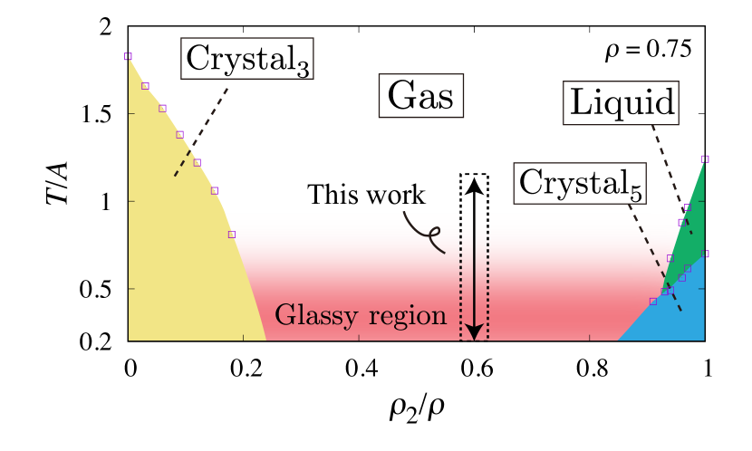
Figure 1: Phase diagram of the model in the plane of temperature $T$ and type-2 particle density $\rho_{2}$ with the total density $\rho=0.75$. Crystal₃ and Crystal₅ stand crystalline phases where a crystal structure is mainly composed of particles with $\ell_{1}=3$ and $\ell_{2}=5$, respectively. The gas, liquid, crystalline phases are separated by first-order phase transitions. In the glassy region, the system shows an aging effect and its autocorrelation function relaxes in two steps. We study the system with $\rho_{2}/\rho=0.6$ in this work.

A lattice glass model we study in this letter is a binary mixture of particles defined by the Hamiltonian with a positive constant $A$

$$H\left({\boldsymbol{n},\boldsymbol{\sigma}}\right)=A\sum_{i=1}^{L^{3}}n_{i}\Big{(}\sum_{j\in\partial i}n_{j}-\ell_{\sigma_{i}}\Big{)}^{2},$$ (1)

where the first summation runs over all the lattice sites. The lattice is the simple cubic lattice with linear dimension $L$. We denote the occupancy of site $i$ with $n_{i}\in\{0,1\}$, and the type of a particle at site $i$ with $\sigma_{i}\in\{1,2\}$. The parameter $\ell_{\sigma_{i}}$ determines the most favorable number of neighboring particles of type $\sigma_{i}$ particle. Here, we consider a binary mixture of $\ell_{1}=3$ and $\ell_{2}=5$ particles. The boundary conditions in all the directions are periodic. We study this model at finite temperature $T$ by Monte Carlo simulation that preserves the number of each type of particles Kawasaki (1966): Two randomly chosen particles are swapped or a randomly chosen particle is moved to a vacant site of the lattice chosen also randomly with the Metropolis probability. Depending on the density of each type of particle, $\rho_{1}$ and $\rho_{2}$, with fixed total density $\rho=\rho_{1}+\rho_{2}=0.75$, our model has crystal phases at low temperature, see Fig. 1. When $\rho_{1}=0.3$ and $\rho_{2}=0.45$, we confirmed the absence of a drop in the energy and a large peak in the specific heat in the glassy region, indicating no crystallization.

Our model is somewhat related to a softened model of a lattice glass proposed by Biroli and Mézard (BM) Biroli and Mézard (2001); Foini et al. (2011). The Hamiltonian of their model $H_{\mathrm{BM}}=A\sum_{i=1}n_{i}\theta\left({\sum_{j\in\partial i}n_{j}-\ell_{\sigma_{i}}}\right)\left({\sum_{j\in\partial i}n_{j}-\ell_{\sigma_{i}}}\right)$ with the Heaviside step function $\theta(x)$. The crucial difference between the two models is the number of neighboring particles that each particle energetically favors: In the soft BM model, any number of neighboring particles lower than $\ell_{\sigma}$ achieves the lowest energy while only $\ell_{\sigma}$ does in our model. This slight change makes the entropy of our model at low temperature smaller than that of the BM model and the dynamics more similar to fragile supercooled liquids.

The dynamics of our model is studied by a local Monte Carlo algorithm Kawasaki (1966), which usually gives dynamics qualitatively similar to molecular and Brownian dynamics. In our simulation, particles can move to only neighboring sites. While any physical quantity of our model relaxes rapidly at high temperature, the relaxation gets extremely slow with decreasing temperature. To quantify the slow dynamics of the model, we study the autocorrelation function

$$C\left({t;t_{\mathrm{w}}}\right)=\Big{\langle}\frac{\frac{1}{N}\sum_{i}\delta_{\sigma_{i}\left({t_{\mathrm{w}}}\right),\sigma_{i}\left({t_{\mathrm{w}}+t}\right)}-C_{0}}{1-C_{0}}\Big{\rangle},$$ (2)

where $t_{\mathrm{w}}$ is the waiting time, $C_{0}=\rho(\rho_{1}^{2}+\rho_{2}^{2})$, $N=\rho L^{3}$ the total number of particles, and the summation is taken over sites with $n_{i}(t_{\mathrm{w}})=1$. We also measure the dynamical susceptibility $\chi_{4}\left({t;t_{\mathrm{w}}}\right)$ characterizing the dynamical heterogeneity observed in supercooled liquids. In the limit $t_{\mathrm{w}}\to\infty$, the system is in equilibrium and we denote $C\left({t}\right)=C\left({t;t_{\mathrm{w}}\to\infty}\right)$ and $\chi_{4}\left({t}\right)=\chi_{4}\left({t;t_{\mathrm{w}}\to\infty}\right)$. We set $t_{\mathrm{w}}$ to a sufficiently large value to study the equilibrium dynamics of the model so that $C\left({t;t_{\mathrm{w}}}\right)$ and $C\left({t;t_{\mathrm{w}}/10}\right)$ agree with each other. Typical values of $t_{\mathrm{w}}$ range from $10^{2}$ to $10^{8}$ Monte Carlo sweeps depending on temperature. Whereas the autocorrelation function of the system decays rapidly at high temperature, a two-step relaxation emerges in $C(t)$ at temperature lower than $T/A\simeq 0.6$, see Fig. 3 (see also Sup for a physical interpretation of the plateau in $C(t)$). The dynamical susceptibility $\chi_{4}(t)$ shows a peak at finite time, indicating the emergence of heterogeneous dynamics of the system Kob et al. (1997); Yamamoto and Onuki (1998); Ediger (2000); Toninelli et al. (2005); Berthier and Biroli (2011). The peak value grows with decreasing temperature (see inset of Fig. 3), and it suggests that the dynamics gets more heterogeneous at lower temperature.

The RFOT theory of the glass transition predicts slow dynamics frozen at a dynamical transition temperature without any thermodynamic anomaly. In the vicinity of the dynamical transition temperature, the relaxation time diverges algebraically. However, an exponentially growing relaxation time well described by the Vogel–Fulcher–Tammann (VFT) law has been observed in experiments of fragile super-cooled liquids. Activated process in finite dimensions is supposed to wipe out the mean-field dynamical transition. Here, we study temperature dependence of the relaxation time $\tau_{\alpha}$ measured as a time when $C\left({t}\right)$ decays to $e^{-1}$. Around temperature where the two-step relaxation emerges, the relaxation time shows a super-Arrhenius growth with decreasing temperature (see Fig. 3). We find that the VFT law fits our data at lower temperatures very well with $T_{\mathrm{VFT}}/A=0.177(6)$ (see also Sup for estimation of the dynamical transition temperature). Note that, as the relaxation time at low temperature increases with the system size, $T_{\mathrm{VFT}}$ would shift to higher temperature in larger systems Sup .

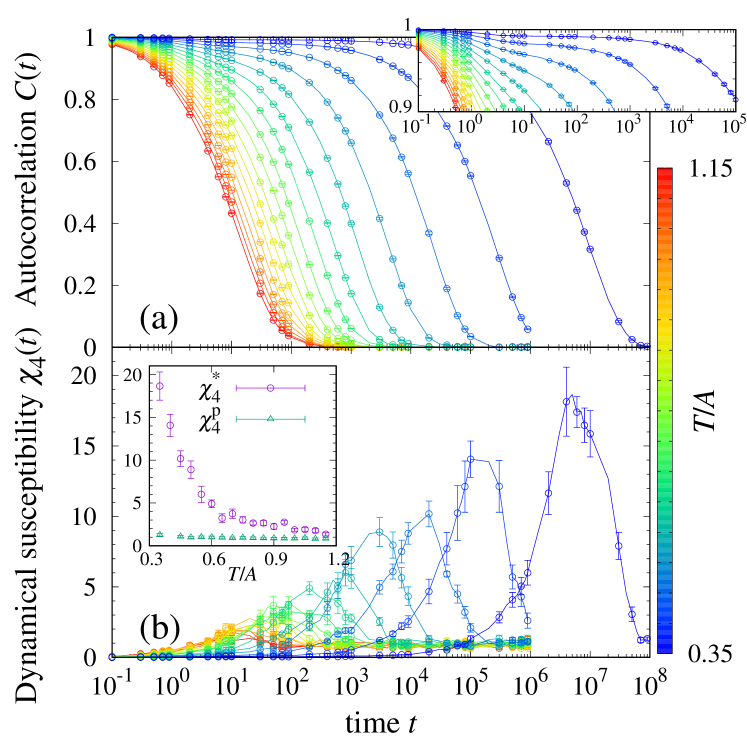
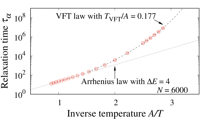
Figure 2: (a) The autocorrelation function of the system. Inset shows an enlarged view around the plateau region. (b) The dynamical susceptibility $\chi_{4}\left({t}\right)$ of the system. Inset shows temperature dependence of the peak and the plateau values of $\chi_{4}\left({t}\right)$ that are denoted as $\chi_{4}^{*}$ and $\chi_{4}^{\mathrm{p}}$, respectively. The system size $N=6000$ ($L=20$).

Figure 3: The Arrhenius plot of the relaxation time $\tau_{\alpha}$ of the system with $N=6000$ ($L=20$). The broken and dotted lines are the Arrhenius law with $\Delta E=4$ and the VFT law with $T_{\rm VFT}/A=0.177$ respectively for guides to eyes.

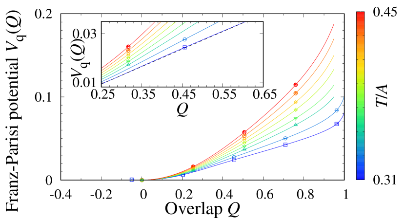
Figure 4: The Franz–Parisi potential $V_{\mathrm{q}}(Q)$ of the system with $N=1296$ ($L=12$). At high temperature the potential is convex while it is slightly non-convex at low temperature, $T/A=0.31$. Inset shows an enlarged view. The broken line is a guide to eyes to show the non-convexity.

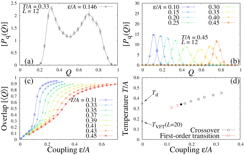
Figure 5: (a, b) The probability distribution of the overlap averaged over quenched reference configurations $[P_{\mathrm{q}}(Q)]$ with finite coupling field $\varepsilon$ at $T/A=0.33$ (a) and $0.45$ (b), respectively. (c) The overlap $[\langle Q\rangle]$ as a function of the field $\varepsilon$. With increasing $\varepsilon$, $[\langle Q\rangle]$ grows smoothly at high temperature while it shows a rapid increase at low temperature. The system size $N=1296$ ($L=12$). (d) Temperature-coupling phase diagram of the system. The empty points and their errors are estimated by the peak of the spin glass susceptibility $\chi_{\mathrm{SG}}$ from the data for $L=12$. The filled circle point represents an expected location of the critical point that is not determined precisely here. The triangular point $T_{\mathrm{VFT}}$ is from the VFT-law fit of the relaxation time for $L=20$, see Fig. 3. The diamond point indicates the dynamical transition temperature $T_{\mathrm{c}}\simeq 0.348(4)$ estimated by fitting Sup .

In the RFOT theory, the overlap between independent replicas has been studied as an order parameter for the thermodynamic glass transition. The overlap successfully detects the glass transition in systems without spatial symmetry Cammarota and Biroli (2012, 2013); Kob and Berthier (2013); Ozawa et al. (2015). The overlap can detect even the slow dynamics at low temperature through its effective free energy Franz and Parisi (1995, 1997, 1998). In our model, however, the overlap and its distribution function can have no anomaly at any temperature due to its spatial symmetry Mézard and Parisi (2012). The temperature dependence of the long-time limiting value of the dynamical susceptibility $\chi_{4}(t\to\infty)$, equivalent to the spin glass susceptibility $\chi_{\mathrm{SG}}$, is indeed almost independent of temperature (see inset of Fig. 3). This is in contrast to a Potts spin glass model Takahashi and Hukushima (2015) where $\chi_{\rm SG}$ increases with approaching its transition temperature Takahashi and Hukushima (shed).

To study rare fluctuations and the effective free energy of the overlap appropriately, we introduce a field $\varepsilon$ in our model: A system at temperature $T$ is coupled by the field to a quenched configuration randomly sampled at the same temperature in equilibrium Franz and Parisi (1995, 1997, 1998). The field explicitly breaks the invariance associated with the spatial symmetry, and thus the overlap can have nontrivial distributions. In the RFOT theory, the field induces a first-order transition at low temperature and the transition terminates at a critical point belonging to the random-field Ising model universality class Franz and Parisi (2013). The Franz–Parisi potential reveals the existence of metastable states at low-temperature and allows us to compute the configurational entropy as a free-energy difference between two minima Berthier and Coslovich (2014); Berthier et al. (2017). Here, we use the Wang–Landau algorithm Wang and Landau (2001a, b) with the multi-overlap ensemble Berg and Janke (1998) to compute the density of states $\Omega_{T}(Q)$ as a function of the overlap $Q$ at a given temperature $T$ with a fixed reference configuration. The Franz–Parisi potential $V_{\mathrm{q}}(Q)$ is computed from $\Omega_{T}(Q)$ by averaging over quenched reference configurations. We prepared reference configurations by equilibrating the system at each temperature for $10^{8}$ Monte Carlo sweeps with non-local swaps of particles. The non-local swap dynamics is faster with a factor of $\sim 10^{2}$ at low temperature than the local swap dynamics while the factor slightly depends on temperature and the system size. The number of reference configurations is $912$ for $T/A=0.31$ and $0.33$, and $48$ for higher temperatures. At high temperature, the potential $V_{\mathrm{q}}(Q)$ is convex and the overlap $[\langle Q\rangle]$ as a function of the field $\varepsilon$ grows gradually, see Fig. 4 and Fig. 5 (c). Here, the brackets $\langle\cdot\rangle$ and $[\cdot]$ represent the thermal and the reference-configuration averages, respectively. At $T/A=0.33$ and $0.31$, the Franz–Parisi potential is slightly non-convex (see Fig. 4), and the probability distribution of the overlap $[P_{\mathrm{q}}(Q)]$ with finite $\varepsilon$ has two separated peaks whereas that at temperature higher than $T/A=0.35$ shows a clear single peak at any $\varepsilon$, see Fig. 5 (a) and (b), respectively . We thus conclude that the coupling field induces a first-order transition into our model that terminates at a critical point at finite temperature as in mean-field and particle models in finite dimensions Franz and Parisi (1997, 1998, 2013); Berthier (2013); Berthier and Jack (2015) (see Fig. 5 (d) for $T$-$\varepsilon$ phase diagram).

When we assume the existence of the thermodynamic glass transition at $T_{\mathrm{K}}>0$ for a system with spatial symmetry, we find the system-size dependence of the effective transition point $\varepsilon_{c}(L)$ and the configurational entropy density $s_{\mathrm{conf}}(L)$ as follows. In the thermodynamic limit, an infinitesimal coupling field should make them have a finite overlap at $T<T_{\mathrm{K}}$ whereas the overlap is strictly zero when $\varepsilon=0$ due to spatial symmetry Mézard and Parisi (2012). In finite systems, the first-order transition at finite field thus never goes to the expected $T_{\mathrm{K}}$, even in the limit $\varepsilon\to+0$, while it may approach zero temperature in the limit. At temperature lower than $T_{\mathrm{K}}$, the effective transition point $\varepsilon_{\mathrm{c}}$ should scale as $\varepsilon_{\mathrm{c}}=O(L^{-a})$ while at higher temperature $\varepsilon_{\mathrm{c}}-\varepsilon_{\mathrm{c}}^{(\infty)}=O(L^{-a})$ where $\varepsilon_{\mathrm{c}}^{(\infty)}=\lim_{L\to\infty}\varepsilon_{\mathrm{c}}(L)>0$ and $a>0$, which depends on systems Fisher and Berker (1982); Mueller et al. (2014). Regarding that the configurational entropy density $s_{\mathrm{conf}}$ measured as the free energy difference in the Franz–Parisi potential is almost equivalent to $\varepsilon_{\mathrm{c}}$, we expect $s_{\mathrm{conf}}$ of finite systems to be finite even below expected $T_{\mathrm{K}}$, but decreases with $\sim L^{-a}$, as $\varepsilon_{\mathrm{c}}(L)$ does. Studying the finite-size dependence of the first-order transition line and the configurational entropy would be a decisive test for the RFOT theory.

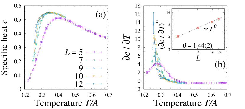
Figure 6: Temperature dependence of (a) the specific heat $c$ and (b) its temperature derivative $\partial c/\partial T$ of the system. Inset of (b) shows the peak value of $\partial c/\partial T$ as a function of $L$.

To measure the thermodynamic properties at low temperature, we use the non-local swap dynamics of randomly chosen pairs of particles and the exchange Monte Carlo (or parallel tempering) method Hukushima and Nemoto (1996) to further enhance equilibration. We also utilize the multiple-temperature reweighting technique Ferrenberg and Swendsen (1988, 1989); Münger and Novotny (1991), which significantly improves the accuracy of Monte Carlo results. Typical number of Monte Carlo sweeps for equilibration range from $10^{8}$ to $10^{11}$ per site depending on the system size.

At temperature $T/A\simeq 0.6$ where the two-step relaxation emerges, the specific heat is rather smooth, and it starts to drop without a divergent behavior at lower temperature (see Fig. 6 (a)). To study further the system-size dependence of the specific heat, we compute the temperature-derivative of the specific heat $\partial c/\partial T$. We find that $\partial c/\partial T$ grows with increasing the system size, indicating that the drop gets steeper with the system size. Similar size-dependence has been observed in a mean-field model with RFOT Billoire et al. (2005) and a three-dimensional Potts glass model that has a RFOT-like spin-glass transition Takahashi and Hukushima (2015).

Assuming the hyperscaling relation of the critical exponents $d\nu=2-\alpha$ with $d$ the spatial dimension, we find that the peak value of $\partial c/\partial T$ follows the finite-size scaling relation

$$\left({\frac{\partial c}{\partial T}}\right)^{*}\propto L^{\theta}$$ (3)

with $\theta=(\alpha+1)/\nu$. We thus can evaluate the two conventional critical exponents from $\theta$ as $\nu=3/\left({\theta+d}\right)$ and $\alpha=2-d\nu=2-3d/\left({\theta+d}\right)$. If the specific heat does not diverge but has a finite jump at a thermodynamic glass transition as in the RFOT theory, the critical exponent $\alpha=0$, suggesting $\nu=2/d$. The peak value $\left({\partial c/\partial T}\right)^{*}$ thus grows algebraically with exponent $\theta=1/\nu=d/2$. This provides a useful way for studying thermodynamic anomaly with a finite-size scaling analysis even when an order parameter is unknown. Here, in our model, the exponent $\theta=1.44(2)$ (see inset of Fig. 6 (b)), implying $\nu=0.68(1)$ and $\alpha=-0.03(1)$, marginally compatible with the RFOT theory.

In summary, we proposed a lattice glass model that is very stable against crystallization and shows the typical dynamics observed in fragile supercooled liquids at low temperature. Our numerical results show that a glass transition is detected by a singularity of the temperature-derivative of the specific heat with exponents compatible with the RFOT theory. We also numerically computed the quenched version of the Franz–Parisi potential using the Wang–Landau algorithm. The potential shows very large overlap fluctuations at low temperature, and a first-order transition was found in the coupled system that terminates at a critical point. The large overlap fluctuations strongly suggest that low-temperature glassy dynamics emerge from thermodynamics of the system, similar to the mean-field models with the RFOT. We thus conclude that our model is useful to study and further examine the mean-field RFOT predictions. Thanks to the lattice nature of our model, it is easy to study its mean-field solution using the cavity method and compare it with our results. To determine precisely the phase diagram both in mean-field and finite dimensions will constitute a crucial test of the validity of the theory.

Supplemental Material for “Lattice glass model in three spatial dimensions” Yoshihiko Nishikawa Koji Hukushima

.1 Supplemental Item 1: Dynamics at low temperature

In off-lattice particle models for supercooled liquids and glasses, the dynamics at low temperature shows two-step relaxation as well as our model. The physical interpretation of the plateau regime in the particle models is well known that particles vibrate locally inside cages effectively formed by surrounding particles Berthier and Biroli (2011). However, since particles of our model defined on a lattice have discrete degrees of freedom, the appropriate physical interpretation analogous to the local vibration in the plateau regime is unclear. In this supplemental item, we show evidence of local vibrations of particles during the plateau regime.

Thanks to the discrete nature of our model, it is easy to find lattice sites that have no contribution to the autocorrelation function Eq. (2), where $\delta_{\sigma_{i}\left({t_{\mathrm{w}}}\right),\sigma_{i}\left({t_{\mathrm{w}}+t}\right)}=0$, i.e. the lattice sites that have different types of particles at $t=0$ and $t>0$ or that are vacant at $t>0$ but occupied at $t=0$. Roughly speaking, a cluster represents a movable region during time interval $t$. We identify connected clusters of those lattice sites at time $t$, and compute the normalized distribution of the cluster size $n_{c}$. Fig. S1 shows the distribution of the connected-cluster size depending on the time $t$ .

At temperature $T/A=0.35$, the autocorrelation function has a plateau from time $t\simeq 10$ to $t\simeq 10^{3}$, see Fig 2. In this time regime, the size of connected clusters $n_{\mathrm{c}}\lesssim 10$, and the distribution is almost independent of time, see Fig. S1. Although the size distribution does not depend on time very much, the positions of the clusters change with time during the plateau, and some of them disappear with time (see Fig. S2 for real-space visualization of the changed lattice sites). We thus conclude, at short time scale $t\lesssim 10^{3}$, the system has local vibrations that involve only $O(1)$ number of particles. These local vibrations produce the plateau in the autocorrelation function, even in the lattice model.

As time passes, the distribution of $n_{\mathrm{c}}$ has a broad tail towards larger $n_{\mathrm{c}}$, and eventually becomes double-peaked at large time $t\simeq\tau_{\alpha}\simeq 10^{7}$. The emergence of two peaks in the distribution with small clusters of $n_{\mathrm{c}}=O(1)$ and giant clusters of $n_{\mathrm{c}}=O(N)$ indicates the heterogeneous dynamics. At time $t=10^{7}$, the largest cluster spreads over the system while there are still some regions where only small clusters occupy, see Fig. S2.

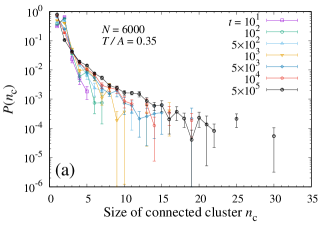
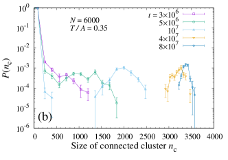
Figure S1: The normalized distribution function of the size of connected clusters at $T/A=0.35$ for (a) $10^{1}\leq t\leq 5\times 10^{5}$ and (b) $3\times 10^{6}\leq t\leq 8\times 10^{7}$. The system size $L=20$ ($N=6000$).

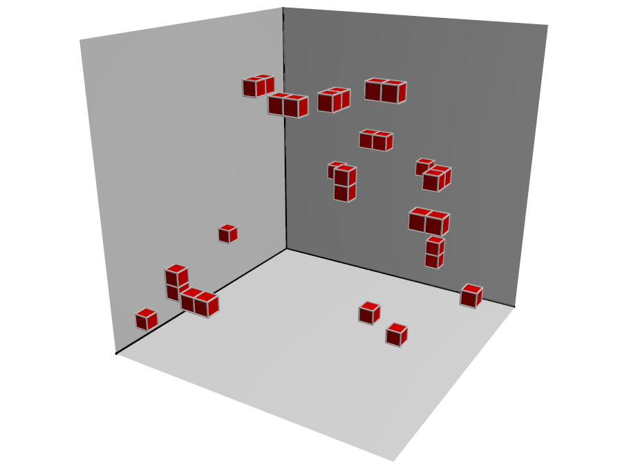
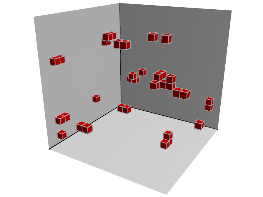
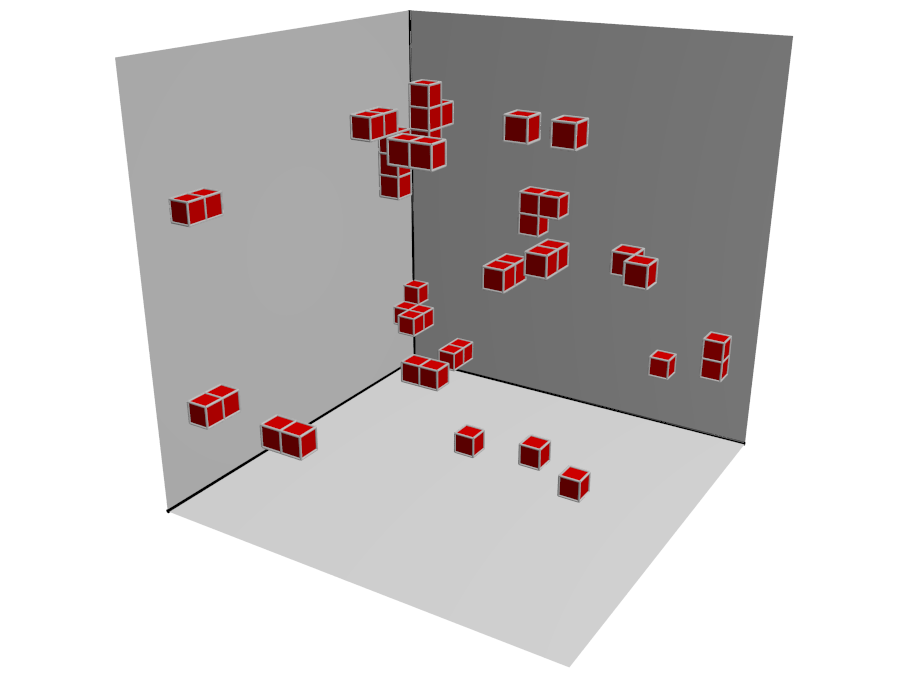
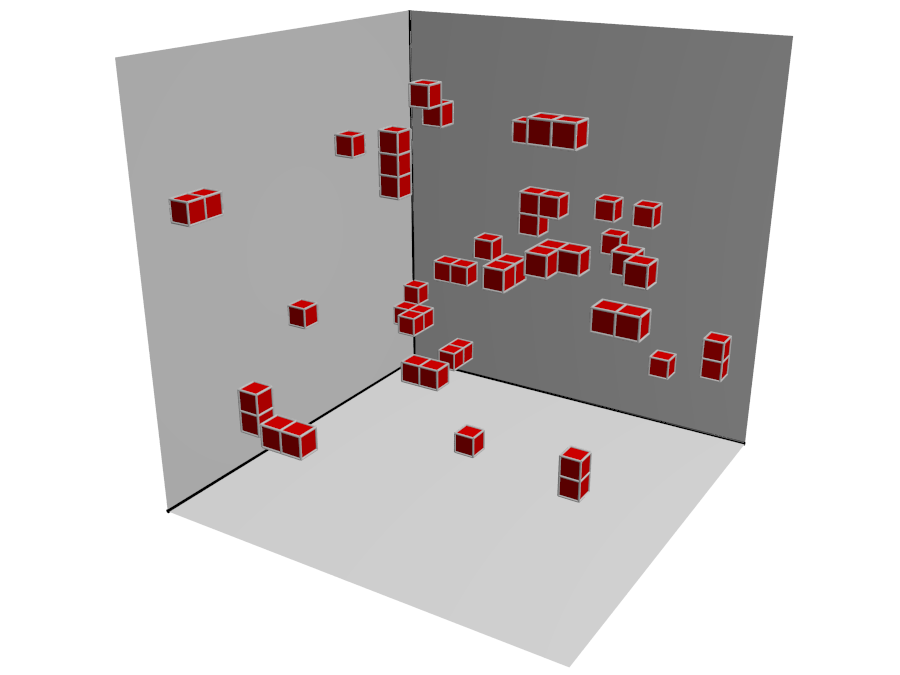
Figure S2: Real-space visualization of typical configurations at time $t=10^{1},10^{2},5\times 10^{2},10^{3}$, and $10^{7}$, from left top to right bottom. The temperature $T/A=0.35$. The lattice sites which have different particles in the configuration at finite time $t>0$ from the original configuration at $t=0$ are filled with cubes. Here, at this temperature, the autocorrelation function has a plateau when $10^{1}\lesssim t\lesssim 10^{3}$. For the configuration at $t=10^{7}$, the lattice sites belonging to the largest connected cluster are filled with blue cubes, and those for the other clusters are filled with red cubes.

.2 Supplemental Item 2: Estimation of the dynamical transition temperature

In the RFOT theory, the relaxation time diverges algebraically at temperature $T_{\mathrm{d}}>T_{\mathrm{K}}$ rather than exponentially as observed in experiments. Whereas the dynamical transition turns into a crossover in finite dimensions, a well-defined localization transition of the potential energy landscape was shown to control the dynamical cross-over Coslovich et al. (2019). However, their method to identify the localization transition is not available in our model. We thus estimate the dynamical transition temperature $T_{\mathrm{d}}$ by a more traditional method, that is, power-law fitting of the relaxation time as done in Ref. Biroli and Mézard (2001).

We show in Fig. S3 the best fit of the inverse relaxation time to a power-law behavior $\sim(T-T_{\mathrm{d}})^{\gamma}$, with $T_{\mathrm{d}}=0.348(4)$ and $\gamma=4.18(12)$. In mean-field models, the dynamical transition temperature is close to the critical temperature of the $\varepsilon$-coupled system Franz and Parisi (1997, 1998, 2013). Our estimation of $T_{\mathrm{d}}$ is compatible with the temperature-coupling phase diagram Fig. 6.

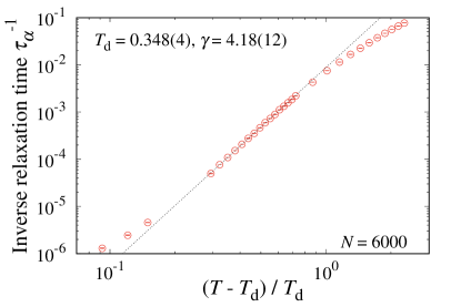
Figure S3: The inverse relaxation time $\tau_{\alpha}^{-1}$ as a function of $(T-T_{\mathrm{d}})/T_{\mathrm{d}}$ and a power-law curve $\sim(T-T_{\mathrm{d}})^{\gamma}$. The dynamical transition temperature $T_{\mathrm{c}}$ and the exponent $\gamma$ are estimated by fitting using the data at $0.4\leq T/A\leq 0.6$, as $T_{\mathrm{d}}=0.348(4)$ and $\gamma=4.18(12)$, respectively.

.3 Supplemental Item 3: Finite-size effect in the relaxation time

The relaxation time of glass forming liquids has a decreasing behavior at moderately low temperature Karmakar et al. (2009); Berthier et al. (2012). The magnitude of the decrease is especially remarkable just below the dynamical transition temperature (or the mode-coupling temperature) Karmakar et al. (2009). In our model, with the local dynamics, the relaxation time does not decrease with the system size even around the dynamical transition temperature $T_{\mathrm{d}}=0.348(3)$, see Fig. S4. At lower temperature, the relaxation time rather increases with the system size. The finite-size effect is more prominent in the relaxation time of the non-local dynamics we used for equilibrium computation, see Fig. S4. Intuitively, the finite-size effect is clearer because of the following reason. The relaxation process at moderately low temperature is mixed with many modes, with each contribution. The slowest mode of the relaxation process, which diverges towards the transition temperature and has strong finite size effects, is buried in many other modes due to its small contribution in the dynamics of inefficient algorithms, including simple local dynamics. The relaxation time shows a finite-size effect only when the slowest mode contribution becomes very large, which is very low temperature. Efficient algorithms, on the other hand, can reduce contributions of modes faster than the slowest mode but still very slow, and thus a finite-size effect that the slowest mode has is seen more clearly. This is actually quite general in other models, even in simple ferromagnetic spin models, by comparing the dynamics of the simple Metropolis algorithm and more efficient algorithms such as the over-relaxation, for instance.

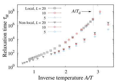
Figure S4: The relaxation time as a function of inverse temperature for $L=5,10$, and $20$ for the local and non-local dynamics. The inverse dynamical transition temperature $A/T_{\mathrm{d}}$ is estimated in Supplemental Item 2.