Abstract

We devise a novel neural network-based universal denoiser for the finite-input, general-output (FIGO) channel. Based on the assumption of known noisy channel densities, which is realistic in many practical scenarios, we train the network such that it can denoise as well as the best sliding window denoiser for any given underlying clean source data. Our algorithm, dubbed as Generalized CUDE (Gen-CUDE), enjoys several desirable properties; it can be trained in an unsupervised manner (solely based on the noisy observation data), has much smaller computational complexity compared to the previously developed universal denoiser for the same setting, and has much tighter upper bound on the denoising performance, which is obtained by a theoretical analysis. In our experiments, we show such tighter upper bound is also realized in practice by showing that Gen-CUDE achieves much better denoising results compared to other strong baselines for both synthetic and real underlying clean sequences.

1 Introduction

Denoising is a ubiquitous problem that lies at the heart of a wide range of fields such as statistics, engineering, bioinformatics, and machine learning. While numerous approaches have been undertaken, many of them focused on the case for which both the input and output of a noisy channel are continuous-valued (Donoho and Johnstone,, 1995; Elad and Aharon,, 2006; Dabov et al.,, 2007). In addition, discrete denoising, in which the input and output of the channel take their values in some finite set, have also been considered more recently (Weissman et al.,, 2005; Moon et al.,, 2016; Moon and Weissman,, 2009).

In this paper, we focus on the hybrid case, namely, the setting in which the underlying clean input source is finite-valued, while the noisy channel output can be continuous-valued. Such scenario naturally occurs in several applications; for example, in DNA sequencing, the finite-valued nucleotides (A,C,G,T) are typically sequenced through observing the continuous-valued light intensities, also known as flowgrams. Other examples can be found in digital communication, in which the finite-valued codewords are modulated, e.g., QAM, and sent via a Gaussian channel, as well as in speech recognition, in which the finite-valued phonemes are observed as continuous-valued speech waveforms. In all of above examples, the goal of denoising is to recover the underlying finite-valued clean input source from the continuous-valued noisy observations.

There are two standard approaches for tackling above problem: supervised learning and Bayesian learning approaches. The supervised learning collects many clean-noisy paired data and learn a parametric model, e.g., neural networks, that maps noisy to clean data. While simple and straightforward, applying supervised learning often becomes challenging for the applications in which collecting underlying clean data is unrealistic. For such unsupervised setting, a common practice is to apply the Bayesian learning framework. That is, assume the existence of stochastic models on the source and noisy channel, then pursue the optimum estimation with respect to the learned joint distribution. Such approach makes sense for the case in which precisely modeling or designing the clean source is possible, e.g., in digital communication, but limitations can also arise when the assumed stochastic model fails to accurately reflect the real data distribution.

As a third alternative, the so-called universal approach has been proposed in (Weissman et al.,, 2005; Dembo and Weissman,, 2005). Namely, while remaining in the unsupervised setting as in the Bayesian learning, the approach makes no assumption on the source stochastic model and instead applies the competitive analysis framework; namely, it focuses on the class of sliding window denoisers and aims to asymptotically achieve the performance of the best sliding window denoiser for all possible sources, solely based on the knowledge on the noisy channel model. The pioneering work, (Weissman et al.,, 2005), devised Discrete Universal DEnoiser (DUDE) algorithm, which handled the finite-input, finite-output (FIFO) setting, and (Dembo and Weissman,, 2005) extended it to the case of finite-input, general-output (FIGO) channels, the setting on which this paper focuses.

While above both universal schemes enjoyed strong theoretical performance guarantees, they both had critical algorithmic limitations. Namely, the original DUDE becomes very sensitive to the selection of a hyperparameter, i.e., the window size $k$, and the generalized scheme for FIGO channel additionally suffered from the prohibitive computational complexity. Recently, (Moon et al.,, 2016; Ryu and Kim,, 2018) employed neural networks in place of a counting vector used in DUDE and showed their schemes can significantly improve the denoising performance and robustness of DUDE. In this paper, we aim to extend the generalized scheme of (Dembo and Weissman,, 2005) for the FIGO channel toward the direction of (Moon et al.,, 2016; Ryu and Kim,, 2018), i.e., utilize neural networks to achieve much faster and better performance. Such extension is not straightforward, as we argue in the later sections, due to the critical difference that the channel has the continuous-valued outputs.

Our contribution is threefold:

• Algorithmic: We develop a new neural network-based denoising algorithm, dubbed as Generalized CUDE (Gen-CUDE), which can run orders of magnitude faster than the previous state-of-the-art in (Dembo and Weissman,, 2005).

• Theoretical: We give a rigorous theoretical analyses on the performance of our method and obtain a much tighter upper bound on the average loss compared to that of (Dembo and Weissman,, 2005).

• Experimental: We compare our algorithm on denoising both the simulated and real source data and show the superb performance compared to other strong baselines.

2 Notations and Problem Setting

We follow (Dembo and Weissman,, 2005) but give more succinct notations. Throughout this paper, we will generally denote a sequence ($n$-tuple) as, e.g., $a^{n}=(a_{1},\ldots,a_{n})$, and $a_{i}^{j}$ referes to the subsequence $(a_{i},\ldots,a_{j})$. We denote the clean, underlying source data as $x^{n}$ and assume each component $x_{i}$ takes a value in some finite set $\mathcal{A}=\{0,\ldots,M-1\}$. The lowercase letters are used to denote the individual sequences or the realization of a random sequence. We assume the noisy channel, denoted as $\mathcal{C}$, is memoryless and is given by the set $\{f_{a}\}_{a\in\mathcal{A}}$, in which $f_{a}$ denoting the density with respect to the Lebesgue measure associated with the channel output distribution for an input symbol $a$. Following states the mild assumption that we make on $\{f_{a}\}_{a\in\mathcal{A}}$ throughout the paper.

Assumption 1

The set of densities $\{f_{a}\}_{a\in\mathcal{A}}$ is a set of linearly independent functions in $L_{1}(\mu)$.

Given above channel $\mathcal{C}$, the noise-corrupted version of the source sequence $x^{n}$ is denoted as $Y^{n}=(Y_{1},\ldots,Y_{n})$. Note we used the uppercase letter to emphasize the randomness in the noisy observation. Now, consider a measurable quantizer $Q:\mathbb{R}\rightarrow\mathcal{A}$, which quantizes the channel output to symbols in $\mathcal{A}$, and the induced channel $\mathbf{\Pi}$, a $M\times M$ channel transition matrix induced by $Q$ and $\{f_{a}\}$. We denote the quantized output of $Y^{n}$ by $Z^{n}$, and the $(x,z)$-th element of $\mathbf{\Pi}$ can be computed as

$$\mathbf{\Pi}(x,z)=\int_{y:Q(y)=z}f_{x}(y)dy.$$ (1)

Note Assumption 1 ensures that $\mathbf{\Pi}$ is an invertible matrix. Moreover, we denote $Z_{i}\triangleq Q(Y_{i})$ as the quantized version of $Y_{i}$.

Given the entire continuous-valued noisy observation $Y^{n}$, the denoiser reconstructs the original discrete input $x^{n}$ with $\hat{X}^{n}=(\hat{X}_{1}(Y^{n}),\ldots,\hat{X}_{n}(Y^{n}))$, where each reconstructed symbol $\hat{X}_{i}(Y^{n})$ takes its value in $\mathcal{A}$. The fidelity of the denoising is measured by the average loss

$$L(x^{n},\hat{X}^{n}(Y^{n}))=\frac{1}{n}\sum_{i=1}^{n}\mathbf{\Lambda}\Big{(}x_{i},\hat{X}_{i}(Y^{n})\Big{)},$$ (2)

in which $\mathbf{\Lambda}\in\mathbb{R}^{M\times M}$ is a per-symbol bounded loss matrix. Moreover, we denote $\mathbf{\Lambda}_{\hat{x}}$ as the $\hat{x}$-th column of $\mathbf{\Lambda}$ and $\Lambda_{\max}=\max_{x,\hat{x}}\mathbf{\Lambda}(x,\hat{x})$.

Then, for a probability vector $\mathbf{P}\in\Delta^{M}$, the Bayes envelope, $U(\mathbf{P})$, is defined to be

$$U(\mathbf{P})\triangleq\min_{\hat{x}\in\mathcal{A}}\sum_{x\in\mathcal{A}}\mathbf{\Lambda}(x,\hat{x})\mathbf{P}(x),$$ (3)

which, in words, stands for the minimum achievable expected loss in estimating the source symbol that is distributed according to $\mathbf{P}$. The argument that achieves (3) is denoted by $\mathcal{B}(\mathbf{P})$, the Bayes response with respect to $\mathbf{P}$. Furthermore, in the later sections, we extend the notion of Bayes response by using $\mathbf{P}$ that is not necessarily a probability vector.

The $k$-th order sliding-window denoisers are the denoisers that are defined by the time-invariant mappings $g_{k}:\mathbb{R}^{2k+1}\rightarrow\mathcal{A}$. That is, $\hat{X}_{i}(Y^{n})=g_{k}(Y_{i-k}^{i+k})$. We also denote the tuple $\mathbf{Y}^{(k)}_{-i}\triangleq(Y_{i-k}^{i-1},Y_{i+1}^{i+k})$ as the $k$-th order context around the noisy symbol $Y_{i}$.

3 Related Work

3.1 DUDE, Neural DUDE and CUDE

A straightforward baseline for the FIGO channel setting is to simply quantize the continuous-valued output and apply the discrete denoising algorithm to estimate the underlying clean source. While such scheme is clearly suboptimal since it significantly discards the information observed in $Y^{n}$, we briefly review the previous work on discrete denoising so that we can build intuitions for devising our algorithm for the FIGO channel.

DUDE was devised by (Weissman et al.,, 2005) and is a two-pass, sliding-window denoiser for the FIFO setting. In discrete denoising, we denote $Z^{n}$ as the finite-valued noisy sequence, $\mathbf{Z}_{-i}^{(k)}\triangleq(Z_{i-k}^{i-1},Z_{i+1}^{i+k})$ as the $k$-th order context around $Z_{i}$, and $\mathbf{\Gamma}$ as the Discrete Memoryless Channel (DMC) transition matrix that induces the noisy sequence $Z^{n}$ from the clean $x^{n}$. Then, the reconstruction of DUDE at location $i$ is defined to be

$$\hat{X}_{i}(\mathbf{Z}_{-i}^{(k)},Z_{i})=\arg\min_{\hat{x}\in\hat{\mathcal{X}}}\hat{\mathbf{p}}_{\text{emp}}(\cdot|\mathbf{Z}_{-i}^{(k)})^{\top}\mathbf{\Gamma}^{\dagger}[\bm{\Lambda}_{\hat{x}}\odot\bm{\gamma}_{Z_{i}}],$$ (4)

in which $\mathbf{\Gamma}^{\dagger}$ is a Moore-Penrose pseudo-inverse of $\mathbf{\Gamma}$ (assuming $\mathbf{\Gamma}$ is full row-rank), $\bm{\gamma}_{z}$ is the $z$-th column of $\mathbf{\Gamma}$, and $\hat{\mathbf{p}}_{\text{emp}}(\cdot|\mathbf{Z}_{-i}^{(k)})\in\mathbb{R}^{|\mathcal{Z}|}$ is an empirical probability vector on $Z_{i}$ given the context $\mathbf{Z}_{-i}^{(k)}$, obtained from the entire noisy sequence $Z^{n}$. That is, for a $k$-th order double-sided context $\mathbf{Z}^{(k)}$, the $z$-th element of $\hat{\mathbf{p}}_{\text{emp}}(\cdot|\mathbf{Z}_{-i}^{(k)})$ becomes

$$\hat{\mathbf{p}}_{\text{emp}}(z|\mathbf{Z}^{(k)})=\frac{|\{j:\mathbf{Z}_{-j}^{(k)}=\mathbf{Z}^{(k)},Z_{j}=z\}|}{|\{j:\mathbf{Z}_{-j}^{(k)}=\mathbf{Z}^{(k)}\}|}.$$ (5)

The main intuition for obtaining (4) is to show that the true posterior distribution can be approximated by using (5) and inverting the DMC channel, $\mathbf{\Gamma}$. That is, the following approximation

$$p(x_{i}|Z_{i-k}^{i+k})\approx\big{(}\bm{\gamma}_{Z_{i}}\odot[\mathbf{\Gamma}^{\dagger\top}\hat{\mathbf{p}}_{\text{emp}}(\cdot|\mathbf{Z}_{-i}^{(k)})]\big{)}_{x_{i}}$$ (6)

holds with high probability with large $n$ (Weissman et al.,, 2005, Section IV.B). Then, for each location $i$, (4) is the $\mathcal{B}(\bm{\gamma}_{Z_{i}}\odot[\mathbf{\Gamma}^{\dagger\top}\hat{\mathbf{p}}_{\text{emp}}(\cdot|\mathbf{Z}_{-i}^{(k)})])$, the Bayes response with respect to the right-hand side of (6). (Weissman et al.,, 2005) showed the DUDE rule, (4), can universally attain the denoising performance of the best $k$-th order sliding window denoiser for any $x^{n}$.

Neural DUDE (N-DUDE) was recently proposed by (Moon et al.,, 2016), and it identified that the limitation of DUDE follows from the empirical count step in (5). Namely, the count happens totally separately for each context $\mathbf{C}$, even if the contexts can be very similar to each other. To that end, N-DUDE implements a single neural network-based sliding-window denoiser such that the information among similar contexts can be shared through the network parameters. That is, N-DUDE defines $\mathbf{p}^{k}_{\texttt{N-DUDE}}(\mathbf{w},\cdot):\mathcal{Z}^{2k}\rightarrow\Delta^{|\mathcal{S}|}$, in which $\mathbf{w}$ stands for the parameters in the network, and $\mathcal{S}$ is a set of single-symbol denoisers, $s:\mathcal{Z}\rightarrow\mathcal{A}$, which map $\mathcal{Z}$ to $\mathcal{A}$. Thus, $\mathbf{p}^{k}_{\texttt{N-DUDE}}(\mathbf{w},\cdot)$ takes the context $\mathbf{Z}_{-i}^{(k)}$ and outputs a probability distribution on the single-symbol denoisers to apply to $Z_{i}$, for each $i$. Note for discrete denoising, $|\mathcal{S}|$ has to be finite, hence the network has the structure of a multi-class classification network.

To train the network parameters $\mathbf{w}$, N-DUDE defines the objective function

$$\mathcal{L}(\mathbf{w},Z^{n})\triangleq \frac{1}{n}\sum_{i=1}^{n}\mathbb{C.E}\Big{(}\mathbf{L}_{\text{new}}^{\top}\mathds{1}_{Z_{i}},\mathbf{p}^{k}_{\texttt{N-DUDE}}(\mathbf{w},\mathbf{C}_{i})\Big{)},$$

in which $\mathbb{C.E}(\mathbf{g},\mathbf{p})$ stands for the (unnormalized) cross-entropy, and $\mathbf{L}_{\text{new}}^{\top}\mathds{1}_{Z_{i}}$ is the pseudo-label vector for the $i$-th location, calculated from the unbiased estimate of the true expected loss which can be computed with $\mathbf{\Lambda}$, $\mathbf{\Gamma}$, and $Z^{n}$ (more details are in (Moon et al.,, 2016)). Note the dependency of the objective function on $Z^{n}$ is highlighted, hence, the training of $\mathbf{w}$ is done in an unsupervised manner together with the knowledge of the channel.

Once the objective function is minimized via stochastic gradient descent, the converged parameter is denoted as $\mathbf{w}^{\star}$. Then, the single-letter mapping defined by N-DUDE for the context $\mathbf{Z}_{-i}^{(k)}$ is expressed as $s_{k,\texttt{N-DUDE}}(\mathbf{Z}_{-i}^{(k)},\cdot)=\arg\max_{s\in\mathcal{S}}\mathbf{p}^{k}_{\texttt{N-DUDE}}(\mathbf{w}^{\star},\mathbf{Z}_{-i}^{(k)})_{s},$ and the reconstruction at location $i$ becomes

$$\hat{X}_{i,\texttt{N-DUDE}}(\mathbf{Z}_{-i}^{(k)},Z_{i})=s_{k,\texttt{N-DUDE}}(\mathbf{Z}_{-i}^{(k)},Z_{i}).$$ (7)

(Moon et al.,, 2016) shows N-DUDE significantly outperforms DUDE and is more robust with respect to $k$.

CUDE was proposed by (Ryu and Kim,, 2018) following-up on N-DUDE, which took an alternative and simpler approach of using neural network to extend DUDE. Namely, instead of using the empirical distribution in (5), CUDE learns a network $\mathbf{p}^{k}_{\texttt{CUDE}}(\mathbf{w},\cdot):\mathcal{Z}^{2k}\rightarrow\Delta^{|\mathcal{Z}|}$, which takes the context $\mathbf{Z}_{-i}^{(k)}$ as input and outputs a prediction for $Z_{i}$, by minimizing $\frac{1}{n}\sum_{i=1}^{n}\mathbb{C.E}(\mathds{1}_{Z_{i}},\mathbf{p}^{k}_{\texttt{CUDE}}(\mathbf{w},\mathbf{Z}_{-i}^{(k)})).$ Thus, the network aims to directly learn the conditional distribution of $Z_{i}$ given its context $\mathbf{Z}_{-i}^{(k)}$. Once the minimizer $\mathbf{w}^{*}$ is obtained, CUDE then simply plugs in $\mathbf{p}^{k}_{\texttt{CUDE}}(\mathbf{w}^{*},\mathbf{Z}_{-i}^{(k)})$ in place of $\hat{\mathbf{p}}_{\text{emp}}(\cdot|\mathbf{Z}_{-i}^{(k)})$ in (4). (Ryu and Kim,, 2018) shows that CUDE outperforms N-DUDE primarily due to the reduced output size of the neural network, i.e., $|\mathcal{Z}|$ vs. $|\mathcal{S}|=|\mathcal{A}|^{|\mathcal{Z}|}$.

3.2 Generalized DUDE for FIGO channel

(Dembo and Weissman,, 2005) extended DUDE algorithm specifically for the FIGO channel case, and we refer to their scheme as Generalized DUDE (Gen-DUDE) from now on. The key challenge arises in the FIGO channel for applying the DUDE framework is that it becomes impossible to obtain an empirical distribution like (5) based on counting for each context, because there are infinitely many possible contexts.

Therefore, by denoting $\mathbf{P}(X_{i}|y_{i-k}^{i+k})\in\Delta^{M}$ as the conditional probability vector on $X_{i}$ given the $(2k+1)$-tuple $y_{i-k}^{i+k}$, Gen-DUDE first identifies that the denoising rule at location $i$ should be the Bayes response

$$\hat{X}_{i}(y^{n})= \ \mathcal{B}(\mathbf{P}(X_{i}\mid y_{i-k}^{i+k}))=\ \mathcal{B}(\mathbf{P}(X_{i},y_{i-k}^{i+k})),$$ (8)

in which the second equality in (8) follows from ignoring the normalization factor of $\mathbf{P}(X_{i}|y_{i-k}^{i+k})\in\Delta^{M}$. Note, $\mathbf{P}(X_{i},y_{i-k}^{i+k})$ is not a probability vector, but the notion of Bayes response still holds. Now, the joint distribution can be expanded as

$$p(X_{i}=a,y_{i-k}^{i+k})=\sum_{u_{-k}^{k}:u_{0}=a}p(X_{i-k}^{i+k}=u_{-k}^{k},y_{i-k}^{i+k})$$

$$= \sum_{u_{-k}^{k}:u_{0}=a}\underbrace{\Big{[}\prod_{j=-k}^{k}f_{u_{j}}(y_{i+j})\Big{]}}_{(a)}\underbrace{p(X_{i-k}^{i+k}=u_{-k}^{k})}_{(b)},$$ (9)

in which term (a) of (9) follows from the memoryless assumption on the channel $\mathcal{C}$. Then, Gen-DUDE approximates term (b) of (9), which is now the distribution on the finite-valued source $(2k+1)$-tuples, by computing the empirical distribution of the quantized noisy sequence $Z^{n}$ and inverting the induced DMC matrix $\mathbf{\Pi}$, both of which are defined in Section 2. Once the approximation for (9) is done, the Gen-DUDE simply computes the Bayes response as in (8) with the approximate joint probability vector. For more details, we refer to the paper (Dembo and Weissman,, 2005).

The main critical drawback of Gen-DUDE is the computation required for approximating (9). Namely, the summation in (9) is over all possible $(2k+1)$-tuples of the source symbols, of which complexity grows exponentially with $k$. Therefore, the running time of the algorithm becomes totally impractical even for the modest alphabet sizes, e.g., 4 or 10, as shown in our experimental results in the later section. Moreover, such exponential dependency on $k$ also appears in the theoretical analyses of Gen-DUDE. That is, it is shown that the upper bound on the probability that the average loss of Gen-DUDE deviates from that of the best sliding-window denoiser is proportional to the doubly exponential term $C^{M^{2k+1}}$, which quickly becomes meaningless for, again, modest size of $M$ and $k$. Motivated by such limiations, we introduce neural networks to efficiently approximate $\mathbf{P}_{X_{i},y_{i-k}^{i+k}}$ and compute the Bayes response to significantly improve the Gen-DUDE method.

4 Main Results

4.1 Intuition for Gen-CUDE

As mentioned above, the Gen-DUDE suffers from high computational complexity due to the expansion given in (9) that requires the summation over the exponentially many (in $k$) terms. The main reason for such expansion in (Dembo and Weissman,, 2005) was to utilize the tools of DUDE for approximating term (b) in (9), which inevitably requires to enumerate all the $2k$-tuple terms. Hence, we instead try to directly approximate $\mathbf{P}(X_{i}|y_{i-k}^{i+k})$ using a neural network.

Our algorithm is inspired by N-DUDE and CUDE, mentioned in Section 3.1, which show much better traits compared to the original DUDE. However, we easily notice that the approach of N-DUDE cannot be applied to the FIGO channel case, because there will be infinitely many single-symbol denoisers $s:\mathcal{Y}\rightarrow\mathcal{A}$. Hence, the output layer of the network should perform some sort of regression, instead of the classification as in N-DUDE, but obtaining the pseudo-label for training in that case is far from being straightforward. Therefore, we take an inspiration from CUDE and develop our Generalized CUDE (Gen-CUDE).

In order to build the core intuition for our method, first consider the quantized noisy sequence $Z^{n}$ and the induced DMC matrix $\mathbf{\Pi}$ (defined in (1)). That is, $Z_{i}=Q(Y_{i})$ where $Q(\cdot)$ is the quantizer introduced in Section 2. Furthermore, denote $\mathbf{P}(X_{0}|y_{-k}^{k})\in\Delta^{M}$ and $\mathbf{P}(Z_{0}|y_{-k}^{k})\in\Delta^{M}$ as the conditional probability vectors of $X_{0}$ and $Z_{0}$ given a $(2k+1)$ tuple $y_{-k}^{k}$ that appear in the noisy observation $Y^{n}$. Also, let $\bm{f}_{X_{0}}(y_{0})\in\mathbb{R}^{M}$ be the vector of density values of which $a$-th element is $f_{a}(y_{0})$. We treat all the vectors as row vectors. The following lemma builds the key motivation.

Lemma 1

Given $y_{-k}^{k}$, the following holds.

$$\mathbf{P}(X_{0}|y_{-k}^{k})\propto[\mathbf{P}(Z_{0}|\mathbf{y}_{-0}^{(k)})\cdot\mathbf{\Pi}^{-1}]\odot\bm{f}_{X_{0}}(y_{0})$$ (10)

Namely, we can compute $\mathbf{P}(X_{0}|y_{-k}^{k})$ up to a normalization constant using the conditional distribution on $Z_{0}$, and the information on the channel $\mathcal{C}$.

Proof: We have the following chain of equalities for the conditional distribution $p(x_{0}|y_{-k}^{k})$:

$$p(x_{0}|y_{-k}^{k})= \frac{p(x_{0},y_{-k}^{k})}{p(y_{-k}^{k})}=\frac{p(x_{0},\mathbf{y}_{-0}^{(k)})f_{x_{0}}(y_{0})}{p(y_{-k}^{k})}$$ (11)

$$= p(x_{0}|\mathbf{y}_{-0}^{(k)})f_{x_{0}}(y_{0})\cdot\frac{p(\mathbf{y}_{-0}^{(k)})}{p(y_{-k}^{k})},$$ (12)

in which the second equality of (11) follows from the memoryless property of the densities $\{f_{a}\}_{a\in\mathcal{A}}$ of $\mathcal{C}$, and $\mathbf{y}_{-0}^{(k)}$ stands for the double-sided context $(y_{-k}^{-1},y_{1}^{k})$. Now, by denoting $z_{0}=Q(y_{0})$ as the quantized version of $y_{0}$, we have the following relation.

$$p(z_{0}|\mathbf{y}_{-0}^{(k)})= \sum_{x_{0}}p(z_{0}|x_{0},\mathbf{y}_{-0}^{(k)})p(x_{0}|\mathbf{y}_{-0}^{(k)})$$

$$= \sum_{x_{0}}\mathbf{\Pi}(x_{0},z_{0})p(x_{0}|\mathbf{y}_{-0}^{(k)}),$$ (13)

in which (13) follows from the channel $\mathcal{C}$ being memoryless and utilizing the notation of the induced DMC matrix, $\mathbf{\Pi}$, defined in (13). Thus, following the row vector notations as mentioned above, we have

$$\mathbf{P}(Z_{0}|\mathbf{y}_{-0}^{(k)})=\mathbf{P}(X_{0}|\mathbf{y}_{-0}^{(k)})\cdot\mathbf{\Pi}.$$ (14)

By inverting $\mathbf{\Pi}$ in (14), and combining with (12) and dropping the term $\frac{p(\mathbf{y}_{-0}^{(k)})}{p(y_{-k}^{k})}$, we have the lemma. ∎

From the lemma, we can see that once we have accurate approximation of the conditional distribution $\mathbf{P}(Z_{0}|\mathbf{y}_{-0}^{(k)})$, then we can apply (10) and obtain the Bayes response with respect to $[\mathbf{P}(Z_{0}|\mathbf{y}_{-0}^{(k)})\cdot\mathbf{\Pi}^{-1}]\odot\bm{f}_{X_{0}}(y_{0})$. Now, following the spirit of CUDE, we utilize neural network to approximate $\mathbf{P}(Z_{0}|\mathbf{y}_{-0}^{(k)})$ from the observed data. We concretely describe our Gen-CUDE algorithm in the next subsection.

4.2 Algorithm Description

Inspired by (10) and CUDE, we try to use a single neural network to learn the $k$-th order sliding window denoiser. First of all, define $\mathbf{p}^{k}(\mathbf{w},\cdot):\mathbb{R}^{2k}\rightarrow\Delta^{M}$ as a feed-forward neural network we utilize. With weight parameter $\mathbf{w}$, the network takes context $\mathbf{y}_{-i}^{(k)}$ as input and send out $\mathbf{P}(Z_{0}|\mathbf{y}_{-i}^{(k)})$ as output. To learn the parameter $\mathbf{w}$, we define the objective function as

$$\mathcal{L}_{\texttt{Gen-CUDE}}(\mathbf{w},Y^{n})\triangleq \frac{1}{n-2k}\sum_{i=k}^{n-k}\mathbb{C.E}\Big{(}\mathds{1}_{Z_{i}},\mathbf{p}^{k}(\mathbf{w},\mathbf{Y}_{-i}^{(k)})\Big{)}.$$

Namely, minimizing $\mathcal{L}_{\texttt{Gen-CUDE}}$ leads to training the network to predict the quantized middle symbol $Z_{i}$ based on the continuous-valued context $\mathbf{Y}_{-i}^{(k)}$, hence, the network can maintain the multi-class classification structure with the ordinary softmax output layer. The minimization is done by the stochastic gradient descent-based optimization methods such as Adam (Kingma and Ba,, 2014). Once the minimization is done, we denote the converged weight vector as $\mathbf{w}^{*}$. Then, by motivated by Lemma 1, we define our Gen-CUDE denoiser as the Bayes response with respect to $[\mathbf{p}^{k}(\mathbf{w}^{*},\mathbf{Y}_{-i}^{(k)})\cdot\mathbf{\Pi}^{-1}]\odot\mathbf{f}_{X_{0}}(Y_{i})$ for each $i$. Following summarizes our algorithm.

Algorithm 1 Gen-CUDE algorithm

0:  Noisy sequence $Y^{n}$, Context size $k$, $\mathcal{C}=\{f_{a}\}_{a\in\mathcal{A}}$, $\mathbf{\Lambda}$, Quantizer $Q(\cdot)$

0:  Denoised sequence $\hat{X}_{\text{NN}}^{n}=\{\hat{X}_{i,\text{NN}}(Y^{n})\}_{i=1}^{n}$

  Obtain the quantized sequence $Z^{n}$ using $Q(\cdot)$

  Compute $\mathbf{\Pi}$ as (1) and initialize $\mathbf{p}^{k}(\mathbf{w},\cdot)$

  Obtain $\mathbf{w}^{*}$ minimizing $\mathcal{L}_{\texttt{Gen-CUDE}}(\mathbf{w},Y^{n})$

  if $i=k+1,\ldots,n-k$ then

     Compute $[\mathbf{p}^{k}(\mathbf{w}^{*},\mathbf{Y}_{-i}^{(k)})\cdot\mathbf{\Pi}^{-1}]\odot\bm{f}_{X_{i}}(Y_{i})$

     $\hat{X}_{i,\text{NN}}(y^{n})=\mathcal{B}\big{(}[\mathbf{p}^{k}(\mathbf{w}^{*},\mathbf{Y}_{-i}^{(k)})\cdot\mathbf{\Pi}^{-1}]\odot\bm{f}_{X_{i}}(Y_{i})\big{)}$

  else

     $\hat{X}_{i,\text{NN}}(Y^{n})=Z_{i}$

  end if

  Obtain $\hat{X}_{\text{NN}}^{n}(Y^{n})=\{\hat{X}_{i,\text{NN}}(Y^{n})\}_{i=1}^{n}$

4.3 Theoretical Analysis

In this subsection, we give a theoretical analysis on Gen-CUDE, which follows similar steps as in (Dembo and Weissman,, 2005) but derives a much tighter upper bound on the average loss of Gen-CUDE. As a performance target for the competitive analysis, we define the minimum expected loss of $x^{n}$ for the $k$th-order sliding-window denoiser by

$$D_{x^{n}}^{k}=\min_{g_{k}}\mathbb{E}\Big{[}\frac{1}{n-2k}\sum_{i=k+1}^{n-k}\mathbf{\Lambda}\Big{(}x_{i},g_{k}\Big{(}Y_{i-k}^{i+k}\Big{)}\Big{)}\Big{]}.$$ (15)

Now, we introduce a regularity assumption to carry out analysis for the performance bound.

Assumption 2

Consider the network parameter $\mathbf{w}^{*}$ learned by minimizing $\mathcal{L}_{\texttt{Gen-CUDE}}$. Then, we assume there exists a sufficiently small $\epsilon^{\prime}>0$ such that

$$\Big{\|}\mathbf{P}(Z_{0}|\mathbf{y}_{-0}^{(k)})-\mathbf{p}^{k}(\mathbf{w}^{*},\mathbf{y}_{-0}^{(k)})\Big{\|}_{1}\leq\epsilon^{\prime}$$

holds for all contexts $\mathbf{y}_{-0}^{(k)}\in\mathbb{R}^{2k}$.

Assumption 2 is based on the universal approximation theorem (Cybenko,, 1989; Hornik et al.,, 1989), which ensures that there always exists a neural network that can approximate any function with arbitrary accuracy. Thus, we assume that the neural network learned by minimizing $\mathcal{L}_{\texttt{Gen-CUDE}}$ results in an accurate enough approximation of the true probability vector $\mathbf{P}(Z_{0}|\mathbf{y}_{-0}^{(k)})$.

Now, by letting

$$\hat{\mathbf{P}}(X_{0}|y_{-k}^{k})\triangleq\frac{p(\mathbf{y}_{-0}^{(k)})}{p(y_{-k}^{k})}[\mathbf{p}^{k}(\mathbf{w}^{*},\mathbf{y}_{-0}^{(k)})\mathbf{\Pi}^{-1}]\odot\mathbf{f}_{X_{0}}(y_{0}),$$

we can then show from Assumption 2 that

$$\mathbb{E}\|\mathbf{P}(X_{0}|Y_{-k}^{k})-\hat{\mathbf{P}}(X_{0}|Y_{-k}^{k})\|_{1}\leq\epsilon^{*},$$ (16)

for $\epsilon^{*}=\epsilon^{\prime}\sum_{a=0}^{M-1}\|\pi_{a}^{-1}\|_{2}$, in which $\mathbb{E}(\cdot)$ is the expectation with respect to $Y_{-k}^{k}$, and $\pi_{a}^{-1}$ stands for the $a$-th column of $\mathbf{\Pi}^{-1}$. The proof of (16) is given Lemma 2 in the Supplementary Material, and it plays an important role in proving the main theorem.

Before stating the main theorem, we first introduce $\mathcal{R}_{\delta}$, which is a quantizer that rounds each component of a probability vector to the nearest integer multiple of $\delta>0$ in $[0,1]$. Then, consider a denoiser $\hat{X}^{n,\delta}_{NN}(Y^{n})$ of which $i$-th component ($k\leq i\leq n-k$) is defined as $\hat{X}_{i,\text{NN}}^{\delta}(Y^{n})=\mathcal{B}(\hat{\mathbf{P}}^{\delta}(X_{i}|Y_{i-k}^{i+k}))$, where $\hat{\mathbf{P}}^{\delta}(X_{i}|Y_{i-k}^{i+k})=\mathcal{R}_{\delta}(\hat{\mathbf{P}}(X_{i}|Y_{i-k}^{i+k}))$. Note when $\delta$ is small enough, the performance of $\hat{X}^{n,\delta}_{\text{NN}}(Y^{n})$ would be close to that of Gen-CUDE. Now, we have the following theorem.

Theorem 1

Consider $\epsilon^{*}$ in (16). Then, for all $k,n\geq 1$, $\delta>0$, and $\epsilon>\Lambda_{\max}\cdot(3\epsilon^{*}+\frac{M\cdot\delta}{2})$, and for all $x^{n}$,

$$\Pr\Big{(} |L_{\hat{X}_{\text{NN}}^{n,\delta}}\left(x^{n},Y^{n}\right)-D_{x^{n}}^{k}|>\epsilon\Big{)}$$

$$\leq C_{1}(k,\delta,M)\exp\Big{(}-\frac{2\left(n-2k\right)}{\left(2k+1\right)}C_{2}(\epsilon,\epsilon^{*},\Lambda_{\max},M,\delta)\Big{)},$$

in which $C_{1}(k,\delta,M)\triangleq 2(2k+1)[\frac{1}{\delta}+1]^{M}$ and $C_{2}(\epsilon,\epsilon^{*},\Lambda_{\max},M,\delta)\triangleq(\epsilon-\Lambda_{\max}\cdot(3\epsilon^{*}+\frac{M\cdot\delta}{2}))^{2}\cdot\frac{1}{\Lambda_{\max}^{2}}$.

Proof: The full proof of the theorem as well as necessary lemmas are given in the Supplementary Material.

Theorem 1 states that for any $x^{n}$, with high probability, Gen-CUDE can essentially achieve the performance of the best sliding-window denoiser with the same order $k$. Note that our bound has the constant term $[\frac{1}{\delta}+1]^{M}$, whereas the paralleling result in (Dembo and Weissman,, 2005) has $[\frac{1}{\delta}+1]^{M^{2k+1}}$. Removing such doubly exponential dependency on $k$ in our result is mainly due to our directly modeling the marginal posterior distribution via neural network, as opposed to the modeling of the joint posterior of the $(2k+1)$-tuple in the previous work. This improvement carries over to the better empirical performance of the algorithm given in the next section.

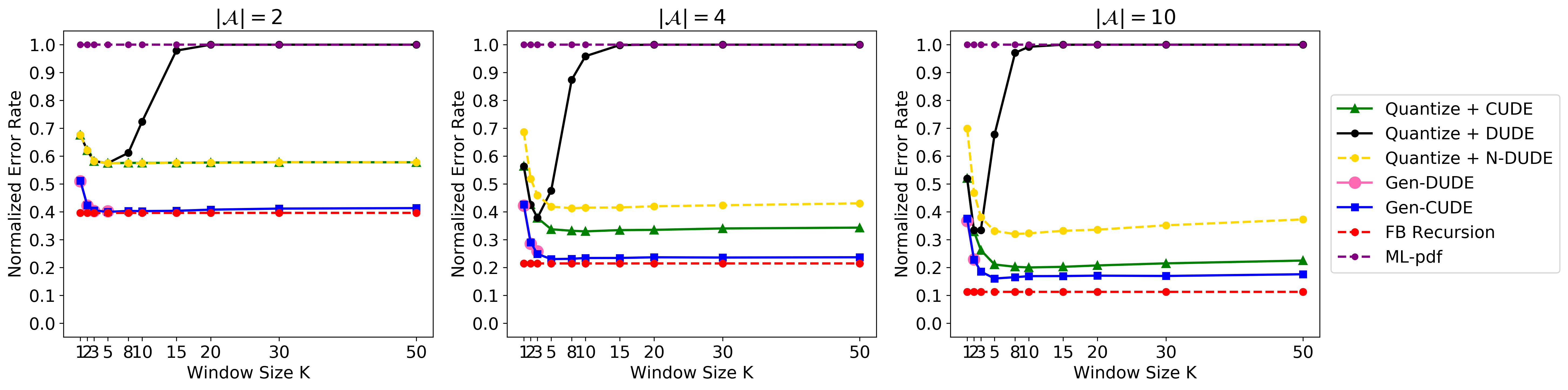
(a) Denoising Performace

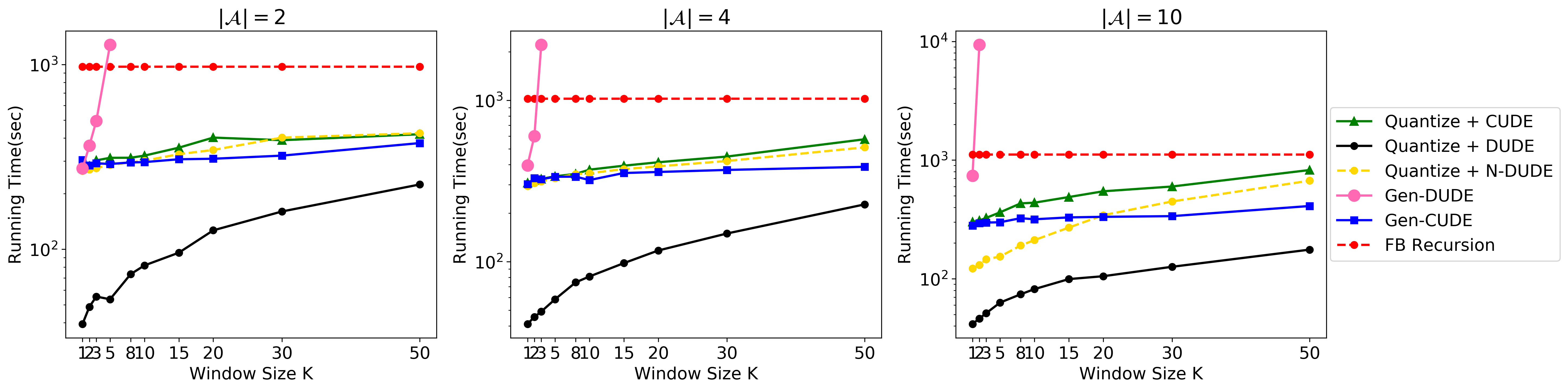
(b) Running Time

Figure 1: Synthetic source data case. (a) Denoising results and (b) running time (including training time). The left, center, and right plots correspond to the case of $|\mathcal{A}|=2$, $4$, and $10$, respectively.

5 Experimental Results

5.1 Setting and baselines

We have experimented with both synthetic and real DNA source data and verified the effectiveness of our proposed Gen-CUDE algorithm. The noisy channel $\mathcal{C}=\{f_{a}\}_{a\in\mathcal{A}}$ was assumed to be known, and the noisy observation $Y^{n}$ was generated by corrupting the source sequence $x^{n}$. We used the Hamming loss as our $\mathbf{\Lambda}$ to measure the denoising performance.

We have compared the performance of Gen-CUDE with several baselines. The simplest baseline is ML-pdf, which carries out the symbol-by-symbol maximum likelihood estimate, i.e., $\hat{X}_{i}(Y^{n})=\arg\max_{a}f_{a}(Y_{i})$. The other baselines are schemes that apply discrete denoising algorithms on the quantized $Z^{n}$ using the induced DMC $\mathbf{\Pi}$. That is, these schemes simply throw away the continuous-valued observation $Y^{n}$ and the density values. We denoted such schemes as Quantized$+$DUDE, Quantized$+$N-DUDE, and Quantized$+$CUDE. We also employed Gen-DUDE as a baseline for FIGO channel. For neural network training, we used a fully-connected network with ReLU (Nair and Hinton,, 2010) activations . For more details on the implementation, the code is available online.

5.2 Synthetic source with Gaussian noise

For the synthetic source data case, we generated the clean sequence $x^{n}$ from a symmetric Markov chain. We varied the alphabet size $|\mathcal{A}|=2,4,10$, and the source symbol was encoded to have odd integer values $\mathcal{O}=\{\pm(2\ell-1):1\leq\ell\leq|\mathcal{A}|/2\}$. The transition probability of the Markov source was set to $0.9$ for staying on the same state and $0.1/|\mathcal{A}|$ for transitioning to the other state. The sequence length was $n=3\times 10^{6}$, and the noisy channel was set to be the standard additive white Gaussian, $\mathcal{N}(0,1)$. The neural network had 6 fully-connected layers and 200 nodes in each layer. For the quantizer $Q(\cdot)$ in all of our experiments, we simply rounded to the nearest integer among $\mathcal{O}$. Note that $Q(\cdot)$ can be freely selected for Gen-CUDE as long as the induced DMC, $\mathbf{\Pi}$, is invertible, and we show the little effect of the choice of $Q(\cdot)$ on the denoising performance in the Supplementary Material.

The denoising performance as well as the running time of each scheme is given in Figure 1, and the performance in Figure 1(a) was normalized with the performance of the simple quantizer, $\hat{X}_{i}=Z_{i}=Q(Y_{i})$. Note for the symmetric Gaussian noise, ML-pdf becomes equivalent to applying $Q(\cdot)$, but they can become different for general noise densities. Moreover, we compared the performance with FB-Recursion (Ephraim and Merhav,, 2002, Section V.), which is the optimal scheme for the given setting since the noisy sequence becomes a hidden Markov process (HMP).

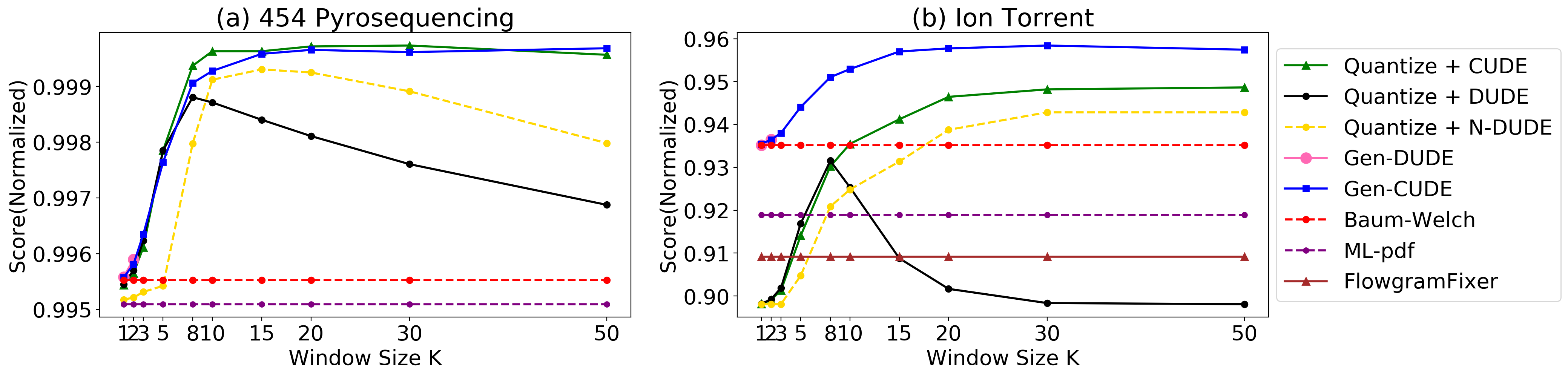
Figure 2: Normalized similarity scores against the clean reference DNA sequence for both sequencing platforms.

From the figures, we can make several observations. Firstly, we note that the neural network-based schemes, i.e., Quantize$+$N-DUDE, Quantize$+$CUDE, and our Gen-CUDE, are very robust with respect to the window size $k$. The effect of the window size $k$ for Gen-CUDE not being huge compared to Gen-DUDE can be predicted from the bound in Theorem 1. In contrast, Quantize$+$DUDE becomes quite sensitive to $k$ as has been identified in (Moon et al.,, 2016). Secondly, we observe our Gen-CUDE always achieves the best denoising performance among the baselines and gets close to the optimal FB-Recursion. Note Gen-CUDE knows nothing about the source sequence $x^{n}$, whereas FB-Recursion exactly knows the source Markov model. Moreover, while Gen-DUDE performs almost as well as Gen-CUDE for $|\mathcal{A}|=2$ with appropriate $k$, its performance significantly deteriorates when the alphabet size grows. We see that the gap between Gen-CUDE and FB recursion widens (although not much) as the alphabet size $M$ increases, which can also be predicted from the bound in Theorem 1. Thirdly, Gen-DUDE suffers from the prohibitive computational complexity as $k$ grows, as shown in Figure 1(b), while the running time of our Gen-CUDE is orders of magnitude faster than that of Gen-DUDE and more or less constant with respect to $k$. From this reason, Gen-DUDE can be run only for small $k$ values. Fourthly, we note Quantize$+$CUDE also performs reasonably well, and it outperforms all discrete denoising baselines as also shown in (Ryu and Kim,, 2018). However, since it discards the additional soft information in the continuous-valued observation and density values, Gen-CUDE, which is tailored for the FIGO channel, outperforms Quantize$+$CUDE with a significant gap.

5.3 DNA source with homopolymer errors

Now, we verify the performance of Gen-CUDE on real DNA sequencing data. We focus on the homopolymer errors which is the dominant error type in “sequencing by synthesis” methods, e.g., Roche 454 pyrosequencing (Quince et al.,, 2011) or Ion Torrent Personal Genome Machine (PGM) (Bragg et al.,, 2013). In those methods, each nucleotide in turn is iteratively washed over with a pre-determined short sequence of bases known as the “wash cycle”, and the continuous-valued flowgrams are observed. Recently, (Lee et al.,, 2017) describes how we can interpret the base-calling procedure of such sequencers exactly as our FIGO channel setting by mapping the DNA sequence into sequence of integers (of homopolymer length), which becomes the input to the noisy channel $\{f_{a}\}_{a\in\mathcal{A}}$, the flowgram densities for each homopolymer length. This interpretation is possible since the order of the nucleotides in the wash cycle is fixed. Denoising in such setting can correct insertion and deletion errors, the dominant and notoriously hard types of errors in such sequencers.

We used Artificial.dat, a public dataset used in (Quince et al.,, 2011) for 454 pyrosequencing, and IonCode0202.CE2R.raw.dat, a data obtained from an internal source, for Ion Torrent after preprocessing both datasets. We simulated the channel of each platform to obtain the noisy sequence that is corrupted with the homopolymer errors. The used noisy channel density was provided for 454, but not for Ion Torrent, hence, we estimated the density for Ion Torrent with a small holdout set with clean source using Gaussian kernel density estimation with bandwidth 0.6. The used densities for 454 and Ion Torrent are shown in the Appendix D of the Supplementary Material. The total sequence length $n$ for 454 and Ion Torrent data was 6,845,624 and 4,101,244, respectively. Moreover, the wash cycle of 454 and Ion Torrent was TACG and TACGTACGTCTGAGCATCGATCGATGTACAGC, respectively. We set the maximum homopolymer length to 9, hence, the source symbol can take values among $\{0,\ldots,9\}$. The neural network for Gen-CUDE had 7 layers with 500 nodes in each layer. After denoising, the error correction performance was compared with the similarity score between the clean reference sequence and the denoised sequence (after converting back from the sequence of homopolymer lengths to the DNA sequence). The score was computed with the Pairwise2 module of Biopython, a common alignment tool to compute the similarity between DNA sequences (Chang et al.,, 2010).

Figure 2 shows the error correction performance for both 454 and Ion Torrent platform data. The score is normalized so that 1 corresponds to the perfect recovery. We also included Baum-Welch (Baum et al.,, 1970) that treats the source as a Markov source and estimates the transition probability before applying the FB-recursion. We can make the following observations. Firstly, we note that Baum-Welch is no longer optimum since the source DNA sequence is far from being a Markov. Secondly, Quantize$+$DUDE, which was used to correct the homopolymer errors in (Lee et al.,, 2017), turns out to be suboptimal, as also observed in Figure 1. Thirdly, Gen-CUDE again achieves the best error correction performance for both 454 and Ion Torrent data. Note for 454, in which the original error rate is quite small, the performance of Quantize$+$CUDE and Gen-CUDE becomes almost indistinguishable, but in Ion Torrent, of which noise density has a higher variance and non-zero means, the performance gap between the two widens. Fourthly, in line with Figure 1, we were not able to run Gen-DUDE for more than $k=2$. Finally, for Ion Torrent, we also run FlowgramFixer (Golan and Medvedev,, 2013), the state-of-the-art homopolymer error correction tool for Ion Torrent, but it showed the worst performance.

6 Conclusion

We devised a novel unsupervised neural network-based Gen-CUDE algorithm, which carries out universal denoising for FIGO channel. Our algorithm was shown to significantly outperform previously developed algorithm for the same setting, Gen-DUDE, both in denoising performance and computation complexity. We also give a rigorous theoretical analyses on the scheme and obtain a tighter upper bound on the average error compared to Gen-DUDE. Our experimental results show promising results, and as a future work, we plan to apply our method to real noisy data denoising and make more algorithmic improvements, e.g., using adaptive quantizers instead of simple rounding.

Appendix A Proof of Theorem 1

The following lemma formalizes to prove Eq. (16) in the paper. First, let $\epsilon^{*}=\epsilon^{\prime}\sum_{a=0}^{M-1}\|\pi_{a}^{-1}\|_{2}$ as shown in the paper and define

$$\hat{\mathbf{P}}(X_{0}|y_{-k}^{k})\triangleq\frac{p(\mathbf{y}_{-0}^{(k)})}{p(y_{-k}^{k})}\cdot[\mathbf{p}^{k}(\mathbf{w}^{*},\mathbf{y}_{-0}^{(k)})\cdot\mathbf{\Pi}^{-1}]\odot\mathbf{f}_{X_{0}}(y_{0}).$$ (17)

Lemma 2

Suppose network parameter $\mathbf{w}^{*}$ learned by minimizing $\mathcal{L}_{\texttt{Gen-CUDE}}$ satisfies Assumption 2. Then,

$$\mathbb{E}\|\mathbf{P}(X_{0}|Y_{-k}^{k})-\hat{\mathbf{P}}(X_{0}|Y_{-k}^{k})\|_{1}\leq\epsilon^{*},$$

in which the expectation is with respect to $Y_{-k}^{k}$.

Proof.

We have the following chain of equations.

$$\mathbb{E}\|\mathbf{P}(X_{0}|Y_{-k}^{k})-\hat{\mathbf{P}}(X_{0}|Y_{-k}^{k})\|_{1}=\int_{\mathbb{R}^{2k+1}}p(y_{-k}^{k})\cdot\|\mathbf{P}(X_{0}|y_{-k}^{k})-\hat{\mathbf{P}}(X_{0}|y_{-k}^{k})\|_{1}\,dy_{-k}^{k}$$

$$=\, \int_{\mathbb{R}^{2k+1}}p(y_{-k}^{k})\cdot\Big{\|}\frac{p(\mathbf{y}_{-0}^{(k)})}{p(y_{-k}^{k})}\cdot[\Big{(}\mathbf{P}(Z_{0}|\mathbf{y}_{-0}^{(k)})-\mathbf{p}^{k}(\mathbf{w}^{*},\mathbf{y}_{-0}^{(k)})\Big{)}\cdot\mathbf{\Pi}^{-1}]\odot\mathbf{f}_{X_{0}}(y_{0})\Big{\|}_{1}\,dy_{-k}^{k}$$ (18)

$$=\, \int_{\mathbb{R}^{2k+1}}p(y_{-k}^{k})\cdot\Big{[}\sum_{a=0}^{M-1}\Big{|}\Big{(}\mathbf{P}(Z_{0}|\mathbf{y}_{-0}^{(k)})-\mathbf{p}^{k}(\mathbf{w}^{*},\mathbf{y}_{-0}^{(k)})\Big{)}\cdot\pi_{a}^{-1}\cdot{f}_{a}(y_{0})\Big{|}\Big{]}\cdot\frac{p(\mathbf{y}_{-0}^{(k)})}{p(y_{-k}^{k})}\,dy_{-k}^{k}$$

$$=\, \sum_{a=0}^{M-1}\int_{\mathbb{R}^{2k+1}}\Big{|}\Big{(}\mathbf{P}(Z_{0}|\mathbf{y}_{-0}^{(k)})-\mathbf{p}^{k}(\mathbf{w}^{*},\mathbf{y}_{-0}^{(k)})\Big{)}\cdot\pi_{a}^{-1}\Big{|}\cdot{f}_{a}(y_{0})\cdot p(\mathbf{y}_{-0}^{(k)})\,dy_{-k}^{k}$$

$$\leq\, \sum_{a=0}^{M-1}\int_{\mathbb{R}^{2k+1}}\Big{\|}\mathbf{P}(Z_{0}|\mathbf{y}_{-0}^{(k)})-\mathbf{p}^{k}(\mathbf{w}^{*},\mathbf{y}_{-0}^{(k)})\Big{\|}_{2}\cdot\|\pi_{a}^{-1}\|_{2}\cdot{f}_{a}(y_{0})\cdot p(\mathbf{y}_{-0}^{(k)})\,dy_{-k}^{k}$$ (19)

$$\leq\, \sum_{a=0}^{M-1}\int_{\mathbb{R}^{2k+1}}\Big{\|}\mathbf{P}(Z_{0}|\mathbf{y}_{-0}^{(k)})-\mathbf{p}^{k}(\mathbf{w}^{*},\mathbf{y}_{-0}^{(k)})\Big{\|}_{1}\cdot\|\pi_{a}^{-1}\|_{2}\cdot{f}_{a}(y_{0})\cdot p(\mathbf{y}_{-0}^{(k)})\,dy_{-k}^{k}$$ (20)

$$\leq\, \epsilon^{\prime}\cdot\sum_{a=0}^{M-1}\Big{[}\|\pi_{a}^{-1}\|_{2}\cdot\int_{\mathbb{R}^{2k+1}}{f}_{a}(y_{0})\cdot p(\mathbf{y}_{-0}^{(k)})\,dy_{-k}^{k}\Big{]}$$ (21)

$$=\, \epsilon^{\prime}\cdot\sum_{a=0}^{M-1}\Big{[}\|\pi_{a}^{-1}\|_{2}\cdot\int_{\mathbb{R}}{f}_{a}(y_{0})\int_{\mathbb{R}^{2k}}p(\mathbf{y}_{-0}^{(k)})\,d\mathbf{y}_{-0}^{(k)}\,dy_{0}\Big{]}=\epsilon^{\prime}\cdot\sum_{a=0}^{M-1}\|\pi_{a}^{-1}\|_{2}=\epsilon^{*},$$ (22)

in which (18) follows from Lemma 1 and (17), (19) follows from the Cauchy-Schwarz inequality, and (20) follows from the fact that $L_{2}$-norm is smaller than the $L_{1}$-norm, and (21) follows from Assumption 2.  ∎∎

Lemma 3

Let $\mathcal{R}_{\delta}(\cdot)$ denote the quantizer that rounds each component of the argument probability vector to the nearest integer multiple of $\delta$ in $(0,1]$. For $M>0$ and $\delta>0$, denote $\hat{\mathbf{P}}^{\delta}$ = $\mathcal{R}_{\delta}(\hat{\mathbf{P}})$. Then,

$$\left\|\hat{\mathbf{P}}^{\delta}\left(X_{0}|y_{-k}^{k}\right)-\hat{\mathbf{P}}\left(X_{0}|y_{-k}^{k}\right)\right\|_{1}\leq\frac{M\cdot\delta}{2}.$$

Proof.

By the definition of $\hat{\mathbf{P}}^{\delta}$, it is clear that

$$\left\|\hat{\mathbf{P}}^{\delta}\left(X_{0}|y_{-k}^{k}\right)-\hat{\textbf{P}}\left(X_{0}|y_{-k}^{k}\right)\right\|_{\infty}\leq\frac{\delta}{2}.$$

Therefore, $$\left\|\hat{\mathbf{P}}^{\delta}\left(X_{0}|y_{-k}^{k}\right)-\hat{\textbf{P}}\left(X_{0}|y_{-k}^{k}\right)\right\|_{1}=\sum_{a=0}^{M-1}|\hat{p}^{\delta}\left(a|y_{-k}^{k}\right)-\hat{p}(a|y_{-k}^{k})|\leq\sum_{a=0}^{M-1}\frac{\delta}{2}\leq\frac{M\delta}{2}.\ \ \qed$$

∎

From Lemma 3, we can expect that for the sufficiently small $\delta$, performance of the denoisers using $\hat{\mathbf{P}}^{\delta}$ and $\hat{\mathbf{P}}$ respectively, for computing the Bayes response will be close to each other.

Lemma 4

Consider $\hat{\mathbf{P}}(X_{0}|Y_{-k}^{k})$ and $\epsilon^{*}$ defined in Lemma 2 and the performance target $D_{x^{n}}^{k}$ defined in Eq. (15) in the paper. Then, we have

$$\Big{|}D_{x^{n}}^{k}-\mathbb{E}_{P_{x^{n}}^{k}\otimes\mathcal{C}}\Big{[}U\Big{(}\hat{\mathbf{P}}({X_{0}|Y_{-k}^{k})}\Big{)}\Big{]}\Big{|}\leq\Lambda_{\max}\cdot\epsilon^{*},$$

in which $P_{x^{n}}^{k}\otimes\mathcal{C}$ stands for the joint distribution on $(X_{0},Y_{-k}^{k})$ defined by the empirical distribution $P_{x^{n}}^{k}(u_{-k}^{k})=\frac{1}{n-2k}\mathbf{r}[x^{n},u_{-k}^{k}]$ with $\mathbf{r}[x^{n},u_{-k}^{k}]=|\{k+1\leq i\leq n-k:x_{i-k}^{i+k}=u_{-k}^{k}\}|$ and the channel density $\mathcal{C}$.

Proof:

First, we identify that

$$\left|D_{x^{n}}^{k}-\mathbb{E}_{P_{x^{n}}^{k}\otimes\mathcal{C}}\Big{[}U\Big{(}\hat{\mathbf{P}}({X_{0}|Y_{-k}^{k})}\Big{)}\Big{]}\right|$$

$$= \left|\mathbb{E}_{P_{x^{n}}^{k}\otimes\mathcal{C}}\Big{[}U\Big{(}\textbf{P}({X_{0}|Y_{-k}^{k})}\Big{)}-\mathbb{E}_{P_{x^{n}}^{k}\otimes\mathcal{C}}[U\Big{(}\hat{\mathbf{P}}({X_{0}|Y_{-k}^{k})}\Big{)}\Big{]}\right|$$ (23)

$$= \int_{\mathbb{R}^{2k+1}}{\mathbb{E}}\Big{[}\mathbf{\Lambda}\Big{(}X,\mathcal{B}(\hat{\mathbf{P}}(X_{0}|y_{-k}^{k}))\Big{)}-\mathbf{\Lambda}\Big{(}X,\mathcal{B}(\mathbf{P}(X_{0}|y_{-k}^{k}))\Big{)}\Big{|}y_{-k}^{k}\Big{]}\cdot p\left(y_{-k}^{k}\right)dy_{-k}^{k},$$ (24)

where the $\mathbb{E}(\cdot)$ in (24) stands for the conditional expectation with respect to $\mathbf{P}(X_{0}|y_{-k}^{k})$, which is the posterior distribution induced from $P_{x^{n}}^{k}\otimes\mathcal{C}$. Now, the following inequality holds for each $y_{-k}^{k}$:

$${\mathbb{E}}\Big{[}\mathbf{\Lambda}\Big{(}X,\mathcal{B}(\hat{\mathbf{P}}(X_{0}|y_{-k}^{k}))\Big{)}-\mathbf{\Lambda}\Big{(}X,\mathcal{B}(\mathbf{P}(X_{0}|y_{-k}^{k}))\Big{)}\Big{|}y_{-k}^{k}\Big{]}$$ (25)

$$= \sum_{a=0}^{M-1}\mathbf{P}(X_{0}=a|y_{-k}^{k})\cdot\Big{[}\mathbf{\Lambda}\Big{(}a,\mathcal{B}(\hat{\mathbf{P}}(X_{0}|y_{-k}^{k}))\Big{)}-\mathbf{\Lambda}\Big{(}a,\mathcal{B}(\mathbf{P}(X_{0}|y_{-k}^{k}))\Big{)}\Big{]}$$ (26)

$$\leq \sum_{a=0}^{M-1}\Big{(}\mathbf{P}(X_{0}=a|y_{-k}^{k})-\hat{\mathbf{P}}(X_{0}=a|y_{-k}^{k})\Big{)}\cdot\Big{[}\mathbf{\Lambda}\Big{(}a,\mathcal{B}(\hat{\mathbf{P}}(X_{0}|y_{-k}^{k}))\Big{)}-\mathbf{\Lambda}\Big{(}a,\mathcal{B}(\mathbf{P}(X_{0}|y_{-k}^{k}))\Big{)}\Big{]}$$ (27)

$$\leq \sum_{a=0}^{M-1}\Big{|}\Big{(}\mathbf{P}(X_{0}=a|y_{-k}^{k})-\hat{\mathbf{P}}(X_{0}=a|y_{-k}^{k})\Big{)}\Big{|}\cdot\Lambda_{\max}=\Lambda_{\max}\cdot\|\textbf{P}(X_{0}|y_{-k}^{k})-\hat{\mathbf{P}}(X_{0}|y_{-k}^{k})\|_{1},$$ (28)

in which (27) follows from the definition of the Bayes response. Therefore,

$$(\ref{eqn_e})\leq\, \Lambda_{\max}\cdot\int_{\mathbb{R}^{2k+1}}\|\textbf{P}(X_{0}|y_{-k}^{k})-\hat{\mathbf{P}}(X_{0}|y_{-k}^{k})\|_{1}\cdot p\left(y_{-k}^{k}\right)dy_{-k}^{k}=\Lambda_{\max}\cdot{\mathbb{E}}\|\textbf{P}(X_{0}|Y_{-k}^{k})-\hat{\mathbf{P}}(X_{0}|Y_{-k}^{k})\|_{1}$$ (29)

$$\leq \Lambda_{\max}\cdot\epsilon^{*},$$ (30)

in which (30) follows from Lemma 2. Note that difference between two expected loss of denoiser based on the Bayes response is bounded with the difference between two probability vectors.  ∎

Lemma 5

Consider $\hat{\mathbf{P}}(X_{0}|Y_{-k}^{k})$ and $\epsilon^{*}$ defined above and define $\hat{\mathbf{P}}^{\delta}=\mathcal{R}_{\delta}(\hat{\mathbf{P}})$ as in Lemma 3. Then,

$$\Big{|}\mathbb{E}_{P_{x^{n}}^{k}\otimes\mathcal{C}}\Big{[}U\Big{(}\hat{\mathbf{P}}(X_{0}|Y_{-k}^{k})\Big{)}-U\Big{(}\hat{\mathbf{P}}^{\delta}\Big{(}X_{0}|Y_{-k}^{k})\Big{)}\Big{]}\Big{|}\leq 2\Lambda_{\max}\cdot\Big{(}\epsilon^{*}+\frac{M\cdot\delta}{4}\Big{)}.$$

Proof.

We have the following chain of inequalities:

$$\Big{|}\mathbb{E}_{P_{x^{n}}^{k}\otimes\mathcal{C}}\Big{[}U\Big{(}\hat{\mathbf{P}}\left(X_{0}|Y_{-k}^{k}\right)\Big{)}\Big{]}-\mathbb{E}_{P_{x^{n}}^{k}\otimes\mathcal{C}}\Big{[}U\Big{(}\hat{\mathbf{P}}^{\delta}\left(X_{0}|Y_{-k}^{k}\right)\Big{)}\Big{]}\Big{|}$$

$$\leq\, \Big{|}\mathbb{E}_{P_{x^{n}}^{k}\otimes\mathcal{C}}\Big{[}U\Big{(}\hat{\mathbf{P}}\left(X_{0}|Y_{-k}^{k}\right)\Big{)}\Big{]}-\mathbb{E}_{P_{x^{n}}^{k}\otimes\mathcal{C}}\Big{[}U\Big{(}\textbf{P}\left(X_{0}|Y_{-k}^{k}\right)\Big{)}\Big{]}\Big{|}$$

$$+\Big{|}\mathbb{E}_{P_{x^{n}}^{k}\otimes\mathcal{C}}\Big{[}U\Big{(}\textbf{P}\left(X_{0}|Y_{-k}^{k}\right)\Big{)}\Big{]}-\mathbb{E}_{P_{x^{n}}^{k}\otimes\mathcal{C}}\Big{[}U\Big{(}\hat{\mathbf{P}}^{\delta}\left(X_{0}|Y_{-k}^{k}\right)\Big{)}\Big{]}\Big{|}$$ (31)

$$\leq\, \Lambda_{\max}\cdot{\mathbb{E}}\|\textbf{P}(X_{0}|Y_{-k}^{k})-\hat{\mathbf{P}}(X_{0}|Y_{-k}^{k})\|_{1}+\Lambda_{\max}\cdot{\mathbb{E}}\|\textbf{P}(X_{0}|Y_{-k}^{k})-\hat{\mathbf{P}}^{\delta}(X_{0}|Y_{-k}^{k})\|_{1}$$ (32)

$$\leq\, 2\Lambda_{\max}\cdot{\mathbb{E}}\|\textbf{P}(X_{0}|Y_{-k}^{k})-\hat{\mathbf{P}}(X_{0}|Y_{-k}^{k})\|_{1}+\Lambda_{\max}\cdot{\mathbb{E}}\|\hat{\textbf{P}}(X_{0}|Y_{-k}^{k})-\hat{\mathbf{P}}^{\delta}(X_{0}|Y_{-k}^{k})\|_{1}$$ (33)

$$\leq\, 2\Lambda_{\max}\cdot{\mathbb{E}}\|\textbf{P}(X_{0}|Y_{-k}^{k})-\hat{\mathbf{P}}(X_{0}|Y_{-k}^{k})\|_{1}+\frac{\Lambda_{\max}\cdot M\cdot\delta}{2}$$ (34)

$$\leq\, 2\Lambda_{\max}\cdot\epsilon^{*}+\frac{\Lambda_{\max}\cdot M\cdot\delta}{2},$$ (35)

in which (Appendix A) follows from the triangular inequality, (32) follows from (29) and replacing $\hat{\mathbf{P}}$ with $\hat{\mathbf{P}}^{\delta}$ in (23), (33) follows from applying the triangular inequality once more, (34) follows from Lemma 3, and (35) follows from (30). Note that probability vectors $\mathbf{P},\hat{\mathbf{P}}$ in Lemma 4 replaced $\hat{\mathbf{P}},\hat{\mathbf{P}}^{\delta}$ in Lemma 5 respectively.   ∎∎

Lemma 6

For every $n\geq 1$, $x^{n}\in\mathcal{A}^{n}$, $\epsilon>0$ and measurable $g_{k}:\mathbb{R}^{2k+1}\rightarrow\mathcal{A}$,

$$\Pr\Big{(}\Big{|}\frac{1}{n-2k}\sum_{i=k+1}^{n-k}\mathbf{\Lambda}\Big{(}x_{i},g_{k}\left(Y_{i-k}^{i+k}\right)\Big{)}-\mathbb{E}_{P_{x^{n}}^{k}\otimes\mathcal{C}}\Big{[}\mathbf{\Lambda}\Big{(}X_{0},g_{k}\left(Y_{-k}^{k}\right)\Big{)}\Big{]}\Big{|}>\epsilon\Big{)}\leq 2(2k+1)\exp\left(-\frac{2\left(n-2k\right)}{\left(2k+1\right)}\epsilon^{2}\cdot\frac{1}{\Lambda_{\max}^{2}}\right).$$

Proof.

We have the following:

$$\Pr\Big{(}\Big{|}\frac{1}{n-2k}\sum_{i=k+1}^{n-k}\mathbf{\Lambda}\Big{(}x_{i},g_{k}\left(Y_{i-k}^{i+k}\right)\Big{)}-\mathbb{E}_{P_{x^{n}}^{k}\otimes\mathcal{C}}\Big{[}\mathbf{\Lambda}\Big{(}X_{0},g_{k}\left(Y_{-k}^{k}\right)\Big{)}\Big{]}\Big{|}>\epsilon\Big{)}$$

$$=\, 2\cdot\Pr\Big{(}\frac{1}{n-2k}\sum_{m=0}^{2k}\sum_{\begin{subarray}{c}i\in\{k+1,\ldots,n-k\},\\ \lceil(i-m)/(2k+1)\rceil=(i-m)/(2k+1)\end{subarray}}\mathbf{\Lambda}\Big{(}x_{i},g_{k}\left(Y_{i-k}^{i+k}\right)\Big{)}-\mathbb{E}_{P_{x^{n}}^{k}\otimes\mathcal{C}}\Big{[}\mathbf{\Lambda}\Big{(}X_{0},g_{k}\left(Y_{-k}^{k}\right)\Big{)}\Big{]}>\epsilon\Big{)}$$

$$\leq\, 2(2k+1)\cdot\Pr\Big{(}\frac{2k+1}{n-2k}\sum_{\begin{subarray}{c}i\in\{k+1,\ldots,n-k\},\\ \lceil i/(2k+1)\rceil=i/(2k+1)\end{subarray}}\mathbf{\Lambda}\Big{(}x_{i},g_{k}\left(Y_{i-k}^{i+k}\right)\Big{)}-\mathbb{E}_{P_{x^{n}}^{k}\otimes\mathcal{C}}\Big{[}\mathbf{\Lambda}\Big{(}X_{0},g_{k}\left(Y_{-k}^{k}\right)\Big{)}\Big{]}>\epsilon\Big{)}$$ (36)

$$\leq\, 2(2k+1)\exp\left(-\frac{2\left(n-2k\right)}{\left(2k+1\right)}\epsilon^{2}\cdot\frac{1}{\Lambda_{\max}^{2}}\right).$$ (37)

Note that if $|i-j|>2k$, $\mathbf{\Lambda}(x_{i},g_{k}(Y_{i-k}^{i+k}))$ is independent from $\mathbf{\Lambda}(x_{j},g_{k}(Y_{j-k}^{j+k}))$. (36) follows from the union bound, and (37) follows from the fact that $\mathbf{\Lambda}(x_{i},g_{k}(Y_{i-k}^{i+k}))-\mathbb{E}_{P_{x^{n}}^{k}\otimes\mathcal{C}}[\mathbf{\Lambda}(X_{0},g_{k}(Y_{-k}^{k}))]$ is a zero-mean, bounded, independent random variable, and the Hoeffding’s inequality. Thus, for every $k$th-order sliding window denoiser, difference between empirical loss and expected loss is vanishing with high probability. ∎∎

Lemma 7

Let $\mathcal{F}_{\delta}^{k}$ denote the set of $\mathcal{A}^{2k+1}$-dimensional vecotrs with components in $[0,1]$ that are integer multiples of $\delta$. Note that $\hat{\mathbf{P}}^{\delta}\in\mathcal{F}_{\delta}^{k}$. Also, let $\mathcal{G}_{\delta}^{k}=\{\mathcal{B}(\mathbf{P})\}_{\mathbf{P}\in\mathcal{F}_{\delta}^{k}}$ be the class of $k$-th order sliding window denoiser defined by computing the Bayes response with respect to $\mathbf{P}\in\mathcal{F}_{\delta}^{k}$. Then, for every $n\geq 1$, $x^{n}\in\mathcal{A}^{n}$, $\epsilon>0$ and $\mathcal{B}(\hat{\mathbf{P}}^{\delta})\in\mathcal{G}_{\delta}^{k}$,

$$\Pr\Big{(}\Big{|}L_{\hat{X}_{\text{NN}}^{\delta}}\left(x^{n},Y^{n}\right)-\mathbb{E}_{P_{x^{n}}^{k}\otimes\mathcal{C}}\Big{[}\mathbf{\Lambda}\Big{(}X_{0},\mathcal{B}(\hat{\mathbf{P}}^{\delta}(X_{0}|Y_{-k}^{k}))\Big{)}\Big{]}\Big{|}>\epsilon\Big{)}\leq\Big{[}\frac{1}{\delta}+1\Big{]}^{M}\cdot 2(2k+1)\exp\left(-\frac{2\left(n-2k\right)}{\left(2k+1\right)}\epsilon^{2}\cdot\frac{1}{\Lambda_{\max}^{2}}\right).$$

Proof.

We have

$$\Pr\Big{(}\Big{|}L_{\hat{X}_{\text{NN}}^{\delta}}\left(x^{n},Y^{n}\right)-\mathbb{E}_{P_{x^{n}}^{k}\otimes\mathcal{C}}\Big{[}\mathbf{\Lambda}\Big{(}X_{0},\mathcal{B}(\hat{\mathbf{P}}^{\delta}(X_{0}|Y_{-k}^{k}))\Big{)}\Big{]}\Big{|}>\epsilon\Big{)}$$

$$=\, \Pr\Big{(}\Big{|}\frac{1}{n-2k}\sum_{i=k+1}^{n-k}\mathbf{\Lambda}\Big{(}x_{i},\mathcal{B}(\hat{\mathbf{P}}^{\delta}(X_{i}|Y_{i-k}^{i+k}))\Big{)}-\mathbb{E}_{P_{x^{n}}^{k}\otimes\mathcal{C}}\Big{[}\mathbf{\Lambda}\Big{(}X_{0},\mathcal{B}(\hat{\mathbf{P}}^{\delta}(X_{0}|Y_{-k}^{k}))\Big{)}\Big{]}\Big{|}>\epsilon\Big{)}$$

$$\leq\, \Pr\Big{(}\max_{g_{k}^{*}\in\mathcal{G}_{\delta}^{k}}\Big{|}\frac{1}{n-2k}\sum_{i=k+1}^{n-k}\mathbf{\Lambda}\Big{(}x_{i},g_{k}^{*}\left(Y_{i-k}^{i+k}\right)\Big{)}-\mathbb{E}_{P_{x^{n}}^{k}\otimes\mathcal{C}}\Big{[}\mathbf{\Lambda}\Big{(}X_{0},g_{k}^{*}\left(Y_{i-k}^{i+k}\right)\Big{)}\Big{]}\Big{|}>\epsilon\Big{)}$$ (38)

$$\leq\, \Big{|}\mathcal{G}_{\delta}^{k}\Big{|}\cdot 2(2k+1)\exp\left(-\frac{2\left(n-2k\right)}{\left(2k+1\right)}\epsilon^{2}\cdot\frac{1}{\Lambda_{\max}^{2}}\right)$$ (39)

$$\leq\, \Big{[}\frac{1}{\delta}+1\Big{]}^{M}\cdot 2(2k+1)\exp\left(-\frac{2\left(n-2k\right)}{\left(2k+1\right)}\epsilon^{2}\cdot\frac{1}{\Lambda_{\max}^{2}}\right),$$ (40)

in which (38) follows from considering the uniform convergence, (39) follows from the union bound, and (40) follows from the crude upper bound on the cardinality $|\mathcal{G}_{\delta}^{k}|$. Note that the window size $k$ in the superscript of upper bound for the cardinality ($[\frac{1}{\delta}+1]^{M}$) is removed compared to that of Gen-DUDE ($[\frac{1}{\delta}+1]^{M^{2k+1}}$). The distinction between them follows from difference in modeling where Gen-CUDE tries to directly model the marginal posterior distribution with neural network rather than the joint posterior of $(2k+1)$-tuple.  ∎∎

Now, we prove our main theorm.

Theorem 1

Consider $\epsilon^{*}$ in Lemma 2. Then, for all $k,n\geq 1$, $\delta>0$, and $\epsilon>\Lambda_{\max}\cdot(3\epsilon^{*}+\frac{M\cdot\delta}{2})$, and for all $x^{n}$,

$$\Pr\Big{(}|L_{\hat{X}_{\text{NN}}^{n,\delta}}\left(x^{n},Y^{n}\right)-D_{x^{n}}^{k}|>\epsilon\Big{)}\leq C_{1}(k,\delta,M)\exp\Big{(}-\frac{2\left(n-2k\right)}{\left(2k+1\right)}C_{2}(\epsilon,\epsilon^{*},\Lambda_{\max},M,\delta)\Big{)},$$

in which $C_{1}(k,\delta,M)\triangleq 2(2k+1)[\frac{1}{\delta}+1]^{M}$ and $C_{2}(\epsilon,\epsilon^{*},\Lambda_{\max},M,\delta)\triangleq(\epsilon-\Lambda_{\max}\cdot(3\epsilon^{*}+\frac{M\cdot\delta}{2}))^{2}\cdot\frac{1}{\Lambda_{\max}^{2}}$.

Proof of theorem 1:

We utilize all the Lemmas given above to prove the theorem. We have

$$\Pr\Big{(}\Big{|}L_{\hat{X}_{\text{NN}}^{\delta}}\left(x^{n},Y^{n}\right)-D_{x^{n}}^{k}\Big{|}>\epsilon\Big{)}$$

$$= \Pr\Big{(}\Big{|}\frac{1}{n-2k}\sum_{i=k+1}^{n-k}\mathbf{\Lambda}\Big{(}x_{i},\mathcal{B}(\hat{\mathbf{P}}^{\delta}(X_{i}|Y_{i-k}^{i+k}))\Big{)}-\mathbb{E}_{P_{x^{n}}^{k}\otimes\mathcal{C}}\Big{[}\mathbf{\Lambda}\Big{(}X_{0},\mathcal{B}(\mathbf{P}(X_{0}|Y_{-k}^{k}))\Big{)}\Big{]}\Big{|}>\epsilon\Big{)}$$ (41)

$$\leq\, \Pr\Big{(}\Big{|}\frac{1}{n-2k}\sum_{i=k+1}^{n-k}\mathbf{\Lambda}\Big{(}x_{i},\mathcal{B}(\hat{\mathbf{P}}^{\delta}(X_{i}|Y_{i-k}^{i+k}))\Big{)}-\mathbb{E}_{P_{x^{n}}^{k}\otimes\mathcal{C}}\Big{[}\mathbf{\Lambda}\Big{(}X_{0},\mathcal{B}(\hat{\mathbf{P}}^{\delta}(X_{0}|Y_{-k}^{k}))\Big{)}\Big{]}\Big{|}$$

$$+\Big{|}\mathbb{E}_{P_{x^{n}}^{k}\otimes\mathcal{C}}\Big{[}\mathbf{\Lambda}\Big{(}X_{0},\mathcal{B}(\hat{\mathbf{P}}^{\delta}(X_{0}|Y_{-k}^{k}))\Big{)}\Big{]}-\mathbb{E}_{P_{x^{n}}^{k}\otimes\mathcal{C}}\Big{[}\mathbf{\Lambda}\Big{(}X_{0},\mathcal{B}(\hat{\mathbf{P}}(X_{0}|Y_{-k}^{k}))\Big{)}\Big{]}\Big{|}$$

$$+\Big{|}\mathbb{E}_{P_{x^{n}}^{k}\otimes\mathcal{C}}\Big{[}\mathbf{\Lambda}\Big{(}X_{0},\mathcal{B}(\hat{\mathbf{P}}(X_{0}|Y_{-k}^{k}))\Big{)}\Big{]}-\mathbb{E}_{P_{x^{n}}^{k}\otimes\mathcal{C}}\Big{[}\mathbf{\Lambda}\Big{(}X_{0},\mathcal{B}(\mathbf{P}(X_{0}|Y_{-k}^{k}))\Big{)}\Big{]}\Big{|}>\epsilon\Big{)}$$ (42)

$$\leq\, \Pr\Big{(}\Big{|}\frac{1}{n-2k}\sum_{i=k+1}^{n-k}\mathbf{\Lambda}\Big{(}x_{i},\mathcal{B}(\hat{\mathbf{P}}^{\delta}(X_{i}|Y_{i-k}^{i+k}))\Big{)}-\mathbb{E}_{P_{x^{n}}^{k}\otimes\mathcal{C}}\Big{[}\mathbf{\Lambda}\Big{(}X_{0},\mathcal{B}(\hat{\mathbf{P}}^{\delta}(X_{0}|Y_{-k}^{k}))\Big{)}\Big{]}\Big{|}>\epsilon-\Lambda_{\max}\cdot(3\epsilon^{*}+\frac{M\cdot\delta}{2})\Big{)}$$ (43)

$$\leq\, \Big{[}\frac{1}{\delta}+1\Big{]}^{M}\cdot 2(2k+1)\exp\left(-\frac{2\left(n-2k\right)}{\left(2k+1\right)}\cdot\Big{(}\epsilon-\Lambda_{\max}\cdot(3\epsilon^{*}+\frac{M\cdot\delta}{2})\Big{)}^{2}\cdot\frac{1}{\Lambda_{\max}^{2}}\right))$$ (44)

$$=\, C_{1}(k,\delta,M)\exp\Big{(}-\frac{2\left(n-2k\right)}{\left(2k+1\right)}C_{2}(\epsilon,\epsilon^{*},\Lambda_{\max},M,\delta)\Big{)},$$ (45)

where (41) follows from the definition of $L_{\hat{X}_{\text{NN}}^{\delta}}(x^{n},Y^{n})$ and $D_{x^{n}}^{k}$, (42) follows from triangle inequality, (43) follows from applying Lemma 5 and Lemma 4, and (44) follows from Lemma 7. Thus, we proved the theorem.  ∎

Appendix B Noise Channel Densities

Here, we show the noisy channel density $\{f_{x}(y)\}_{x\in\mathcal{O}}$ used for the experiments in Section 5.2 and Section 5.3 of the paper. Figure 3 shows the channel densities for the synthetic data experiments in Section 5.2, and Figure 4 shows the channel densities for the 454 and Ion Torrent data experiments in Section 5.3.

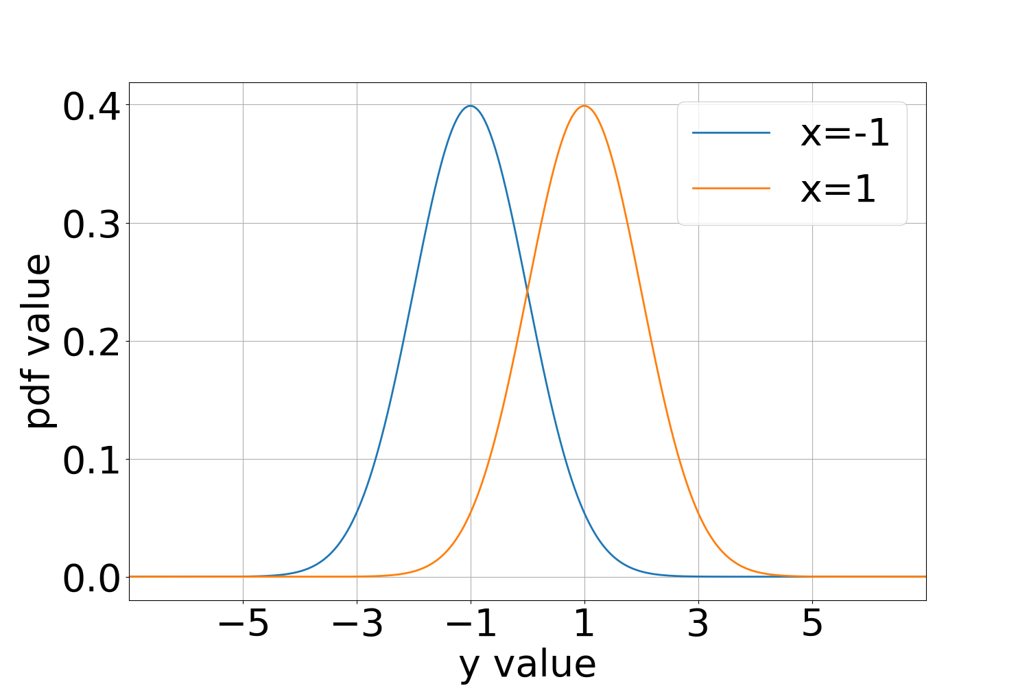
(a) $|\mathcal{A}|=2$

(b) $|\mathcal{A}|=4$

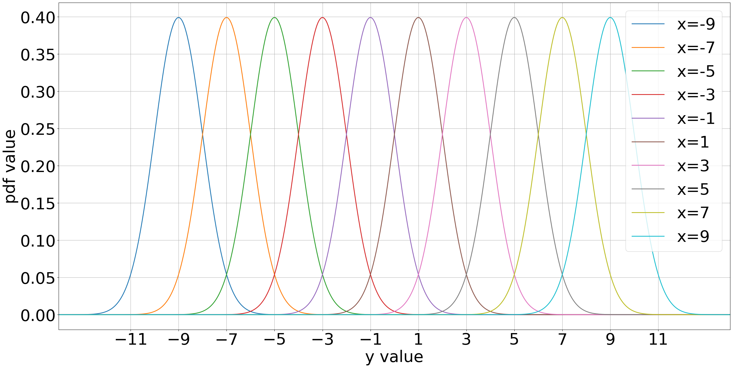
(c) $|\mathcal{A}|=10$

Figure 3: Noisy channel densities used for the synthetic data experiments.

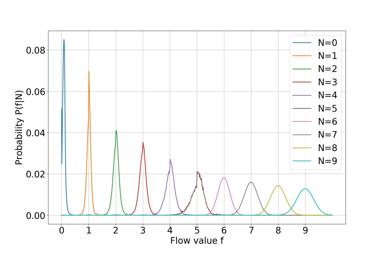
(a) 454 Pyrosequencing

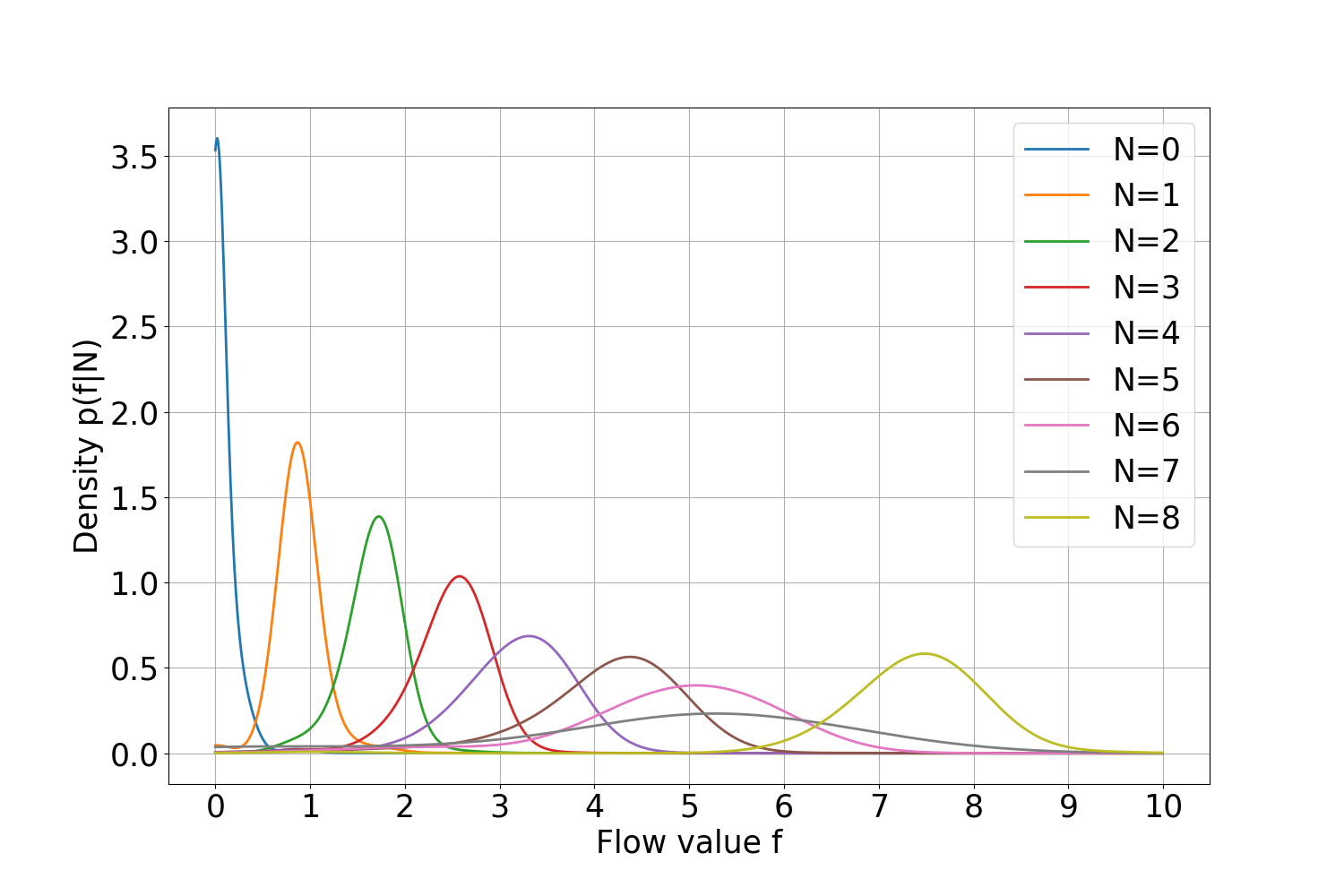
(b) Ion Torrent

Figure 4: Probability ensities of the flowgram-values for the homopolymer lengths in each DNA sequencer. For Ion Torrent, we estimated channel density using Gaussian kernel density estimation with bandwidth=0.6 on the separated holdout dataset.

Appendix C Normalized Error Rate Graph for DNA Experiments

Figure 5 shows the denoising performance measured by the Hamming loss. Note the similarity score in the paper is computed after converting the integer-valued denoised sequence (homopolymer length) back to a DNA sequence. We observe the error patterns are similar to those in Figure 2 of the paper.

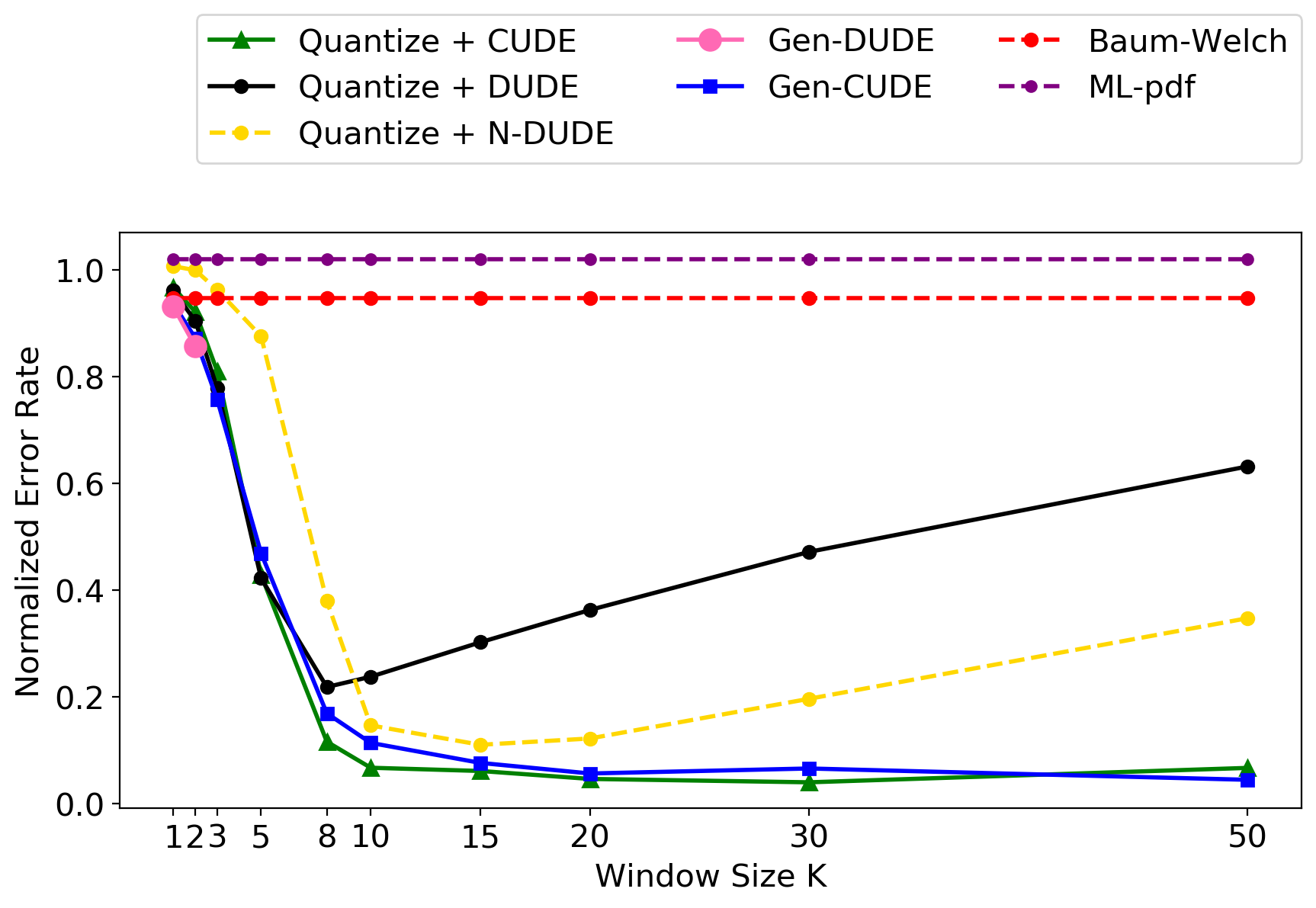
(a) 454 Pyrosequencing

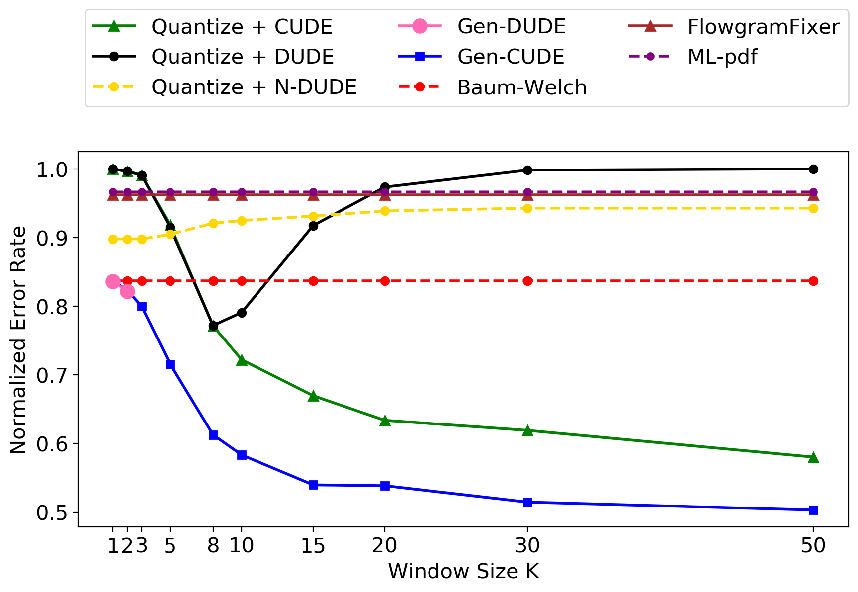
(b) Ion Torrent

Figure 5: Normalized error rate for DNA source data.

Appendix D Error Rate Graph for Randomized Quantizers

We note that the quantizer $Q(\cdot)$ can be freely selected for Gen-CUDE as long as the induced DMC, $\Pi$, is invertible. To show the small effect of the quantizer to the final denoising performance, we designed two additional experiments for the $|\mathcal{A}|=4$ case of Figure 1(a) in the paper. As described in the first paragraph of Section 5.2, the source symbol was encoded as $\{+3,+1,-1,-3\}$ and the decision boundaries of the original $Q(\cdot)$ was $\{-2,0,+2\}$.

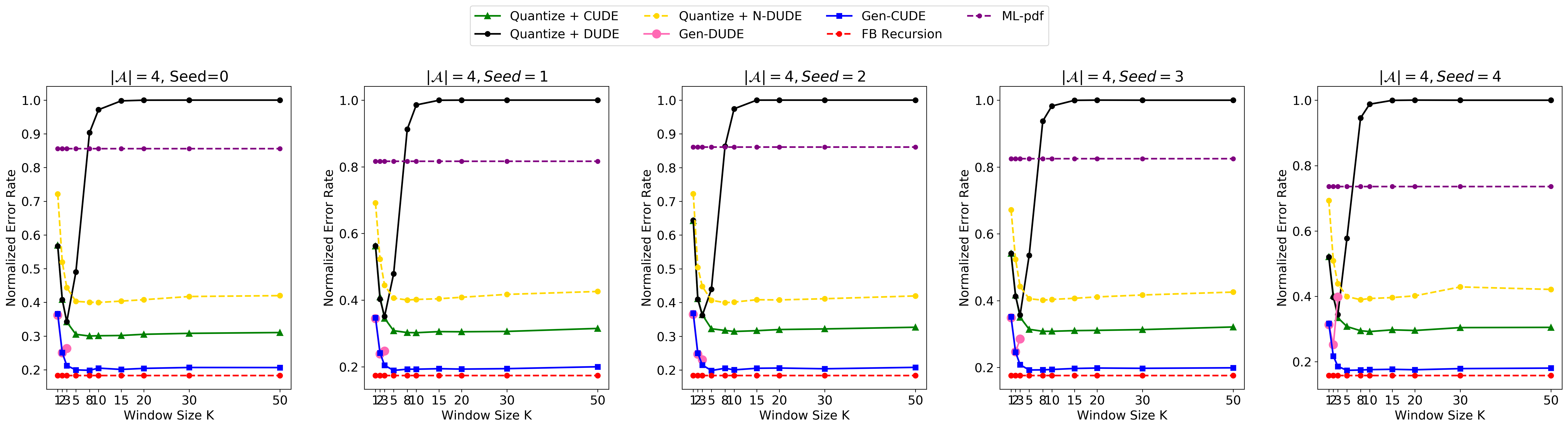
(a) Normalized Error Rate

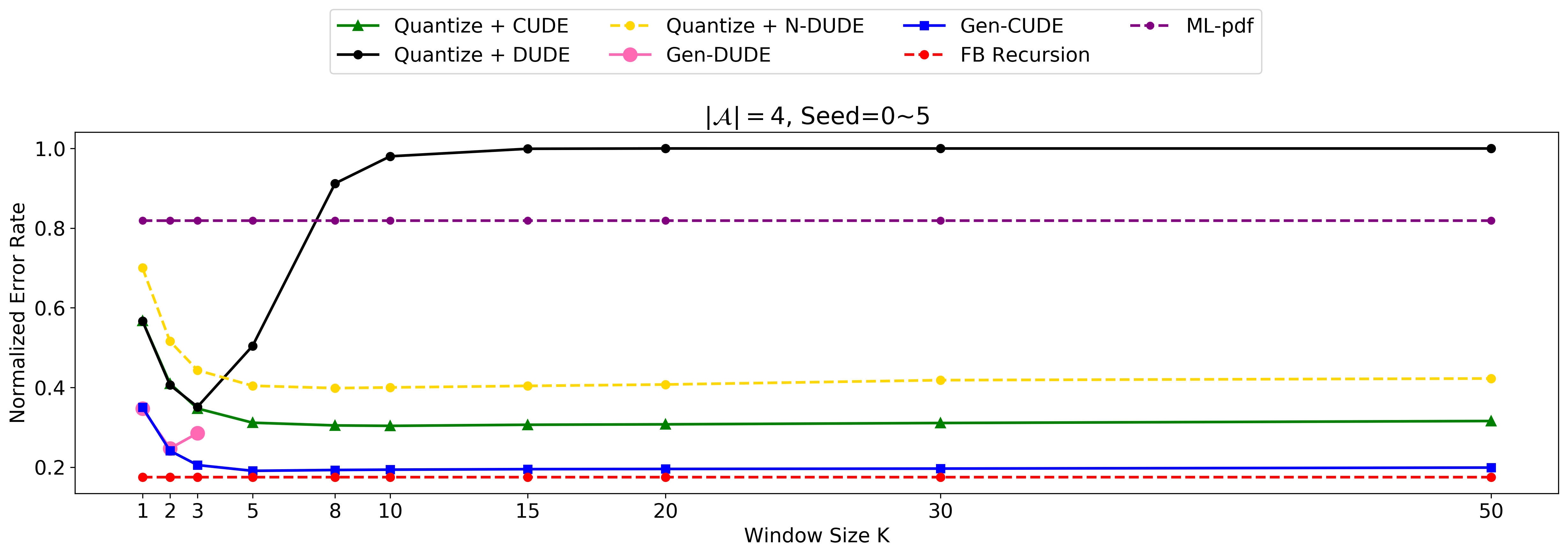
(b) Average Error Rate

Figure 6: Error Rate for Five Randomized Quantizers

In Figure 6(a), we show the results of using five randomized quantizers, of which decision boundaries were obtained by uniform sampling from the intervals, $[-3,-1],[-1,+1],[+1,+3]$, respectively. The 5 different resulting quantizers’ decision boundaries were the following:

• Seed 0 : $[-1.59,0.73,2.09]$

• Seed 1 : $[-1.18,0.27,2.46]$

• Seed 2 : $[-2.29,-0.59,2.49]$

• Seed 3 : $[-1.96,-0.41,1.12]$

• Seed 4 : $[-1.13,0.81,1.61]$.

The five figures in Figure 6(a) show the performance for each quantizer, and Figure 6(b) shows the average error rate of them, which looks quite similar the one shown in Figure 1(a). We can clearly observe that the different quantizers have little effect in the final denoising performance for Gen-CUDE. In contrast, we observe that Gen-DUDE or Quantize+DUDE have more sensitivity to the choice of the quantizer.

Furthermore, we note that our Gen-CUDE does not require to have the same number of the quantized symbols as the input symbols, either. In such cases, the $\mathbf{\Pi}^{-1}$ can be simply replaced with a pseudo-inverse as long as $\mathbf{\Pi}$ has full row-rank. Figure 7 is the result of averaging the performances of using five randomized quantizers, of which decision boundaries are randomly selected from the intervals $[-2.7,-2.3]$, $[-1.7,-1.3]$, $[-0.7,-0.3]$, $[0.3,0.7]$, $[1.3,1.7]$, $[2.3,2.7]$, respectively. (Thus, $Q(\cdot)$ has 7 regions.) The used boundaries are as following:

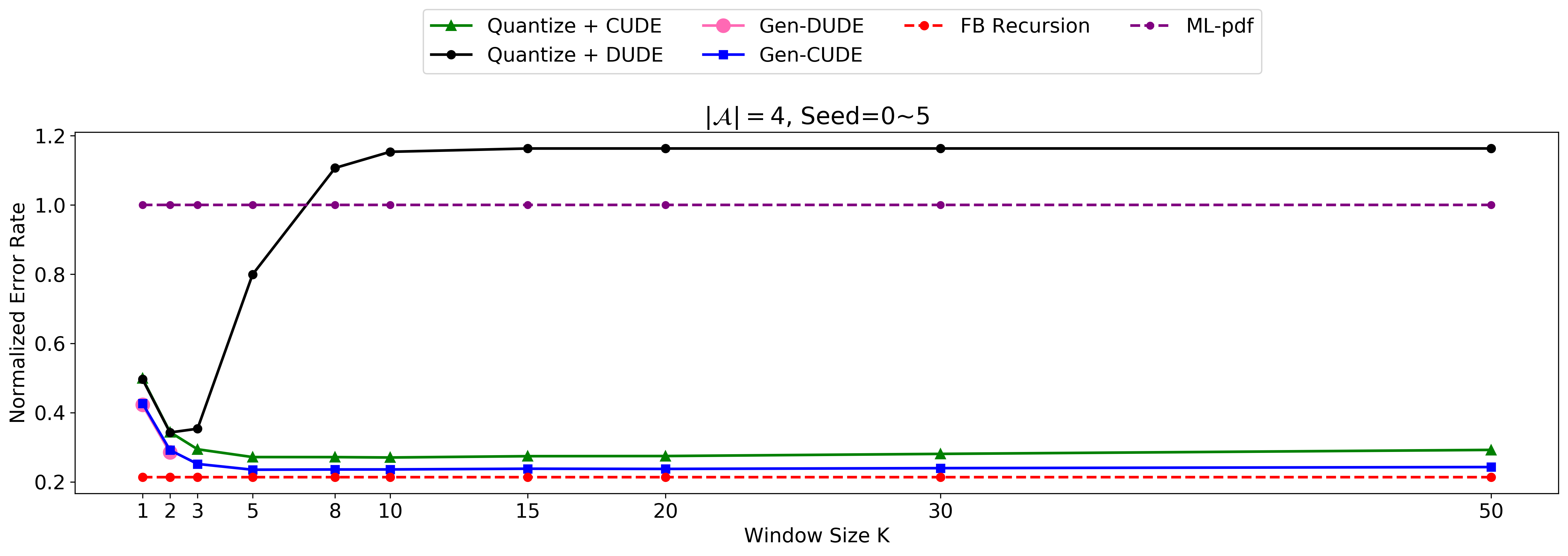
Figure 7: Average Error Rate for Non-square Channel Matrix Case

• Seed 0 : $[-2.42,-1.35,-0.48,0.57,1.44,2.36]$

• Seed 1 : $[-2.34,-1.45,-0.41,0.55,1.55,2.32]$

• Seed 2 : $[-2.56,-1.62,-0.4,0.59,1.56,2.55]$

• Seed 3 : $[-2.49,-1.58,-0.68,0.59,1.49,2.51]$

• Seed 4 : $[-2.33,-1.34,-0.58,0.5,1.67,2.64].$

Again, we see little difference in the performance for Gen-CUDE compared to Figure 7 and Figure 1(a) ($|\mathcal{A}|=4$ case) in the manuscript.

References

• Baum et al., (1970) Baum, L., Petrie, T., Soules, G., and Weiss, N. (1970). A maximization technique occuring in the statistical analysis of probabilistic functions of Markov chains. Annals of Mathematical Statistics, 41(164-171).
• Bragg et al., (2013) Bragg, L. M., Stone, G., Butler, M. K., Hugenholtz, P., and Tyson, G. W. (2013). Shining a light on dark sequencing: characterising errors in ion torrent pgm data. PLoS computational biology, 9(4):e1003031.
• Chang et al., (2010) Chang, J., Chapman, B., Friedberg, I., Hamelryck, T., De Hoon, M., Cock, P., Antao, T., and Talevich, E. (2010). Biopython tutorial and cookbook. Update, pages 15–19.
• Cybenko, (1989) Cybenko, G. (1989). Approximation by superposition of a sigmoidal function. Math. Control Systems Signals, 2(4):303–314.
• Dabov et al., (2007) Dabov, K., Foi, A., Katkovnik, V., and Egiazarian, K. (2007). Image denoising by sparse 3-d transform-domain collaborative filtering. IEEE Trans. Image Processing, 16(8):2080–2095.