Topological Interface between Pfaffian and anti-Pfaffian Order in $\nu=5/2$ Quantum Hall Effect

Abstract

Recent thermal Hall experiment pumped new energy into the problem of $\nu=5/2$ quantum Hall effect, which motivated novel interpretations based on formation of mesoscopic puddles made of Pfaffian and anti-Pfaffian topological orders. Here, we study an interface between the Pfaffian and anti-Pfaffian states, which may play crucial roles in thermal transport, by means of state-of-the-art density-matrix renormalization group simulations on the cylinder geometry. We provide compelling evidences that indicate the edge modes of the Pfaffian and anti-Pfaffian state strongly hybridize with each other around the interface. Moreover, we demonstrate an intrinsic electric dipole moment emerges at the interface, similar to the “p-n” junction sandwiched between N-type and P-type semiconductor. Importantly, we elucidate the topological origin of this dipole moment, whose formation is to counterbalance the mismatch of guiding-center Hall viscosity of bulk Pfaffian and anti-Pfaffian state.

The $\nu=5/2$ fractional quantum Hall (FQH) effect in the second Landau level has sparked much interest in condensed matter for decades Willett et al. (1987); Pan et al. (1999, 2008); Choi et al. (2008); Dolev et al. (2008); Radu et al. (2008); Bid et al. (2010); Willett et al. (2013); Stern et al. (2010); Tiemann et al. (2012); Baer et al. (2014); Venkatachalam et al. (2011), mainly due to its likely non-Abelian nature and potential application in topological quantum computation Kitaev (2003); Nayak et al. (2008). The leading theoretical candidate is the non-Abelian Pfaffian (Pf) state Moore and Read (1991); Greiter et al. (1991), a fully polarized chiral p-wave state of composite fermions Read and Green (2000), as supported by numerical studies Morf (1998); Rezayi and Haldane (2000); Wan et al. (2006); Hu et al. (2009); Möller and Simon (2008); Peterson et al. (2008); Wang et al. (2009); Wójs et al. (2010); Storni et al. (2010); Feiguin et al. (2008); Storni and Morf (2011); Pakrouski et al. (2015); Zhu et al. (2016). Besides, its particle-hole conjugate partner, known as the anti-Pfaffian (APf) state Levin et al. (2007); Lee et al. (2007), is an equally valid candidate, which may actually be more viable under realistic experimental conditions Zaletel et al. (2015a); Rezayi (2017). Breaking of particle-hole symmetry, either spontaneously or explicitly, is crucial for the emergence of the Pf or APf state. Recently, to interpret the observation of half-integer thermal Hall conductance that is consistent with particle-hole symmetry Banerjee et al. (2018), the particle-hole preserved Pf state was proposed Zucker and Feldman (2016); Chen et al. (2014). Alternatively, the experimental observation could be simply explained by lack of thermal equilibration at the edgeSimon (2018a) (a scenario currently under debate Feldman (2018); Simon (2018b)), or more significantly, by the presence of random domains made of the Pf and APf states Mross et al. (2018); Wang et al. (2018); Lian and Wang (2018), similar to an earlier proposal of spontaneously formed Pf and APf strips Wan and Yang (2016). The latter makes understanding of Pf-APf domain walls an urgent priority.

Generally speaking, the topologically protected edge states directly reflect bulk topological order via the bulk-edge correspondence Wen (2004); Keski-Vakkuri and Wen (1993); Li and Haldane (2008); Qi et al. (2012), rendering edge the preferred window to peek into the fascinating bulk physics in topological states of matter Das Sarma et al. (2005); Stern and Halperin (2006); Bonderson et al. (2006); Fendley et al. (2006). In the particular case of non-Abelian Pf-type states, this correspondence leads to the presence of neutral Majorana fermion modes at the edge Milovanović and Read (1996) (i.e. the interface separating the bulk from vacuum) responsible for the half-integer quantized thermal Hall conductanceBanerjee et al. (2018). Relatively speaking less attention is drawn to the interface between two distinct topological states Sandler et al. (1998); Kapustin and Saulina (2011); Kitaev and Kong (2012); Barkeshli et al. (2013); Levin (2013); Lu and Lee (2014); Cano et al. (2015); Yang (2017); Santos et al. (2018); Crépel et al. (2019a, b); Jaworowski and Nielsen (2019), especially for those separating two non-Abelian orders Grosfeld and Schoutens (2009); Bais et al. (2009); Barkeshli et al. (2015); Wan and Yang (2016). Existing theoretical attempts mostly rely on the effective field theories, where novel phenomena may emerge through the coupling between the two edges that meet at the interface. While such phenomenological theory is good at obtaining a qualitative understanding of the possible phases, many open questions remain and call for quantitative study by unbiased numerical approaches Crépel et al. (2019a, b). For example, it is extremely difficult for effective theories to determine which interface state is energetically favored by the microscopic interactions, as well as non-universal aspects like edge reconstructionChamon and Wen (1994); Wan et al. (2002, 2003) which in principle could also happen at the interface Yang (2017). Numerical simulation is expected, in a quantitative and unbiased way, to overcome these challenges faced by effective field theories. It is therefore highly desirable and urgent to develop an advanced numerical scheme, to address some pressing problems like the Pf-APf interface.

In this paper, we construct an interface between the Pf and APf state, based on which we investigate the underlying physics of Pf-APf domain wall in the FQH effect at the filling factor $\nu=5/2$. Our approach is based on a design of cylinder geometry, by utilizing the density-matrix renormalization group (DMRG) algorithm. We establish that the edge modes of the Pf and APf state strongly hybridize near the interface, indicating that counter-propagating charge modes are fully gapped out. Moreover, we identify the appearance of charge inhomogeneity around the interface, which yields a robust electric dipole moment. Crucially, we identify the mismatch of Hall viscosity between the Pf and APf topological orders as the driving force behind this dipole moment, thus revealing the topological content of the Pf-APf interface, whose possible experimental consequences will be discussed.

Model and Method.— We consider interacting electrons in the presence of a perpendicular magnetic field on the cylinder geometry. In the Landau gauge $\mathbf{A}=(0,Bx)$, the single-particle orbital in N-th Landau level is $\psi_{m}(x,y)=\frac{1}{\sqrt{2^{N}N!L_{y}\ell\sqrt{\pi}}}e^{ik_{m}y}e^{-\frac{(x-k_{m}\ell^{2})^{2}}{2\ell^{2}}}H_{N}(\frac{x-k_{m}\ell^{2}}{\ell})$, where the momentum along the circumference is $k_{m}=\frac{2\pi m}{L_{y}}$ and $m$ labels the orbital center position $x_{m}=k_{m}\ell^{2}$ along the cylinder axis ($\ell=\sqrt{\hbar/eB}$ is the magnetic length). When the magnetic field is strong, by projecting onto the second Landau level, the many-body Hamiltonian is written as (see Ref. supple )

$$\hat{H} = \sum_{\{m_{i}\}}V_{m_{1},m_{2},m_{3},m_{4}}\hat{a}^{\dagger}_{m_{1}}\hat{a}^{\dagger}_{m_{2}}\hat{a}_{m_{3}}\hat{a}_{m_{4}}$$ (1)

where $a^{\dagger}_{m}(a_{m})$ is the creation (annihilation) operator of an electron in the orbital $m$, and $V$ represents matrix elements of modified Coulomb interaction $\frac{1}{r}e^{-\frac{r^{2}}{\xi^{2}}}$ with a regulated length $\xi=4\ell$ Zaletel et al. (2015b). Throughout the paper, total filling fraction is set to be half-filled in the second Landau level (on top of the fully occupied first Landau level).

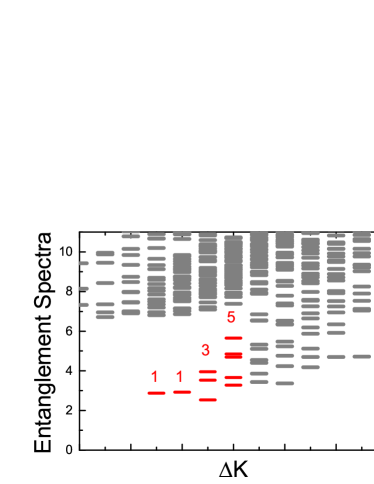
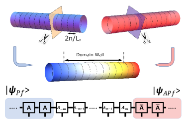
Figure 1: Interface between the Pf and APf topological order on the cylinder geometry. (Top) Typical orbital entanglement spectra for gapped Pf (left) and APf (right) state. The chiral dispersions revealed in the entanglement spectra reflect spontaneous breaking of particle-hole symmetry. (Middle) Schematic representation of the Pf-APf interface in the Landau orbital (labeled as black circle) space on the cylinder geometry. We first cut the Pf (APf) state into two halves, and glue the left part of Pf state and right part of APf state together, which creates an interface regime sandwiched between Pf and APf state. (Bottom) The MPS representation of the Pf-APf interface.

For numerical calculations, we apply a suitable DMRG algorithm with multiple steps for such an interface system. The DMRG algorithm is based on the matrix product state representation of the ground state: $|\Psi(\mathrm{A}^{[n_{m}]}_{m})\rangle=...\mathrm{A}^{[n_{0}]}_{0}\mathrm{A}^{[n_{1}]}_{1}...|...,n_{0},n_{1},...\rangle$, where $\mathrm{A}^{[n_{m}]}_{m}$ are $D\times D$ matrices and $\{n_{m}\}=0,1$ represents the occupancy on orbital $m$. In order to model the interface, we perform the “cut-and-glue” scheme, by combining finite DMRG White (1992) and infinite DMRG McCulloch (2008) algorithms, as discussed below. First, the infinite DMRG is used to iteratively minimize ground state energy $E_{0}=\langle\Psi(\mathrm{A}^{[n_{m}]}_{m})|\hat{H}|\Psi(\mathrm{A}^{[n_{m}]}_{m})\rangle$ by optimizing $\mathrm{A}^{[n_{m}]}_{m}$ on an infinite cylinder Zaletel et al. (2013), which allows us to obtain optimized Pf or APf state separately. The infinite DMRG algorithm has proven to be efficient in the study of FQH ground states ranging from Abelian to non-Abelian systems Zaletel et al. (2013, 2015b); Zhu et al. (2015). Second, based on optimized Pf and APf state living on the infinite cylinder, we cut both of them into two halves, and then glue $\mathrm{A}^{[n_{m}]}_{m}$ ($m<0$) from the Pf state (shaded in blue) together with $\mathrm{A}^{[n_{m}]}_{m}$ ($m\geq 0$) from the APf state (shaded in red), which yields an interface between the Pf and APf state (as graphically shown in Fig. 1). Third, by fixing the end of Pf (APf) state as the left (right) boundary, we optimize the state on a finite segment enclosing $L_{M}$ orbitals (up to $L_{M}=234$) embedded in the middle of the infinite cylinder.

Here we would like to point out methodological advantages of our scheme. First, on the infinite cylinder the Pf and APf states are automatically selected resulting from spontaneous particle-hole symmetry breaking, and are treated on equal footing without empirical knowledge. Second, one can use established techniques, e.g. entanglement spectra via a cylinder bipartition Li and Haldane (2008); Zhu et al. (2016); Zaletel et al. (2015b), as a probe of the Pf (APf) topological order (see Fig. 1(top)). Third, the microscopic state of the interface can be resolved accurately. Our calculation is based on a microscopic Hamiltonian instead of model wave functions Crépel et al. (2019a, b), so the domain wall structure shown below represents the energetically favorable state at the interface.

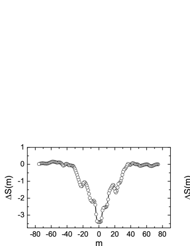
Figure 2: Interface structures distinguished by entanglement entropy. The interface structure in the weak coupling limit (top left) and in the strong hybridization case (top right). Here black dashed lines represent the neutral chiral Majorana fermion modes, solid lines represent chiral boson modes of different kinds (for details see supple ). (Bottom) The calculated entanglement entropy $\Delta S(m)=S(m)-S_{\textrm{Pf(APf)}}$ dependence on bipartition position $m$. ($m=0$ is the center of the interface.) The entanglement entropy develops a dip in the weak coupling limit (bottom left), and a peak structure in the strong hybridization case (bottom right). The cylinder perimeter is set to be $L_{y}=19\ell$ and bond dimension is $D=3600$.

Interface structure.— We start by discussing the effective edge theories of the Pf and APf state Wen and Zee (1992); Keski-Vakkuri and Wen (1993); Milovanović and Read (1996); Levin et al. (2007) (for details see Ref. supple ). There are two possible edge structures across the interface depending on the strength of coupling between them Barkeshli et al. (2015). If tunneling effect across the interface is irrelevant, the edge modes of the Pf and APf state form two (nearly) independent sets, sitting on the left and right side of the interface (see Fig. 2 (top left)). In this case, if an entanglement measurement is performed, we expect a minimum of the entanglement entropy at the interface, reflecting the effectively decoupled nature between the Pf and APf state. On the other hand, if the tunneling process across the interface is strong, the counter-propagating charge modes gap out due to the hybridization effect. As a result, the Pf-APf interface hosts four co-propagating neutral majorana modes Mross et al. (2018); Wang et al. (2018); Lian and Wang (2018); Wan and Yang (2016) (see Fig. 2(top right)), allowing neutral fermion to directly tunnel across the interface. Thus, we expect to see a single smooth peak of entanglement entropy centered at the interface.

Motivated by this intuition, we compute the entanglement entropy and its dependence on the entanglement cut position, by partitioning the cylinder into two parts at different cut position. We first create uncoupled edges, by turning off interaction terms acrossing the interface. In this case, we observe a dip in entanglement at the interface (Fig. 2(bottom left)). As a comparison, the result with full (translationally invariant) interaction is shown in Fig. 2(bottom right). Far away from the interface, the entanglement entropy converges to the value of the Pf (APf) state. Near the interface, the entanglement entropy develops a peak centered at the interface. The appearance of enhanced entanglement across the interface favors the strong coupling picture (Fig. 2(top right)), and suggests that charged modes are fully gapped out and only neutral modes survive around the Pf-APf interface (see supple ).

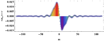
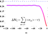
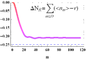
Figure 3: Domain wall structure at the interface. (Top) The charge distribution profile $\langle n_{m}\rangle-\nu$ (open circles) along the cylinder axis. The colored shade denotes the deviation from uniform distribution $\nu=1/2$. The leftmost (rightmost) side is a uniform Pf (APf) state. (Bottom) The integration of the difference between the actual occupation number and the uniform occupation number on the left half $\Delta N_{L}$ (left) and on the right half $\Delta N_{R}$ (right). The cylinder perimeter is set to be $L_{y}=19\ell$ and bond dimension is $D=3600$.

Intrinsic interface dipole moment and Hall viscosity.— In spite of the absence of charged modes, we identify emergent charge fluctuation around the interface. Fig. 3(top) shows the charge distribution along the cylinder axis. One salient feature is that charge profile smoothly interpolates between the Pf and the APf state, and a profound charge fluctuation appears around the interface with small ripples in the periphery of the interface. In particular, we identify that the Pf (APf) side contains an excess of electron(hole)-like chargers. (The electron(hole)-rich region switches, if we swap the position of Pf (APf) state in Fig. 1.) For quantitative description, Fig. 3(bottom) depicts the accumulation of charge on the left and right side of the interface. We find several notable features. First, total charge on the left (right) part of the interface gives $\Delta N_{L}\approx-\Delta N_{R}$ (in unit of $e$), where we define the net charge accumulation as $\Delta N_{L(R)}=\sum_{m\lessgtr 0}[\langle n_{m}\rangle-\nu]$. Importantly, the total charge on each side of the interface is equal but takes opposite sign, which results in a neutral charge condition without net charge accumulation. Second, in this particular case the net charge on the left (right) side is very close to $\pm e/4$ for a quasi-electron (quasi-hole) as expected for the Pf (APf) state. Third, we can also identify the domain wall region with a spatial length scale $d_{\textrm{Pf}}+d_{\textrm{APf}}$, and $d_{\textrm{Pf}}(d_{\textrm{APf}})$ is the distance that domain wall penetrates into the Pf (APf) side. In Fig. 3(bottom), we estimate $d_{\textrm{Pf}}\approx d_{\textrm{APf}}\sim 8\ell$. The obtained spatial penetration depth is slightly larger than previous estimation of quasi-hole radii based on the Pf model wave function Wu et al. (2014). Lastly, we would like to point out, the above finding is similar to that of the “p-n” junction in semiconductor, where the neutrality is lost near the p-n interface and the mobile charge carriers form the depletion layer. Interestingly, different from the p-n junction, next we will show the origin of charge inhomogeneity at the Pf-APf interface is topological.

We first try to gain some physical intuition of the appearance of electric charge inhomogeneity by considering the thin-torus limit Bergholtz and Karlhede (2005); Bernevig and Haldane (2008). The typical root configuration pattern of the Pf state is $...01100110...$, corresponding to a generalized Pauli principle of no more than two electrons in four consecutive orbitals. The APf root configuration is simply its particle-hole conjugate. In order to switch from one pattern to the other, defects must be introduced near the interface, and the simplest one that does not change particle number is $...0110011_{\times}0|1_{\circ}0011001...$, where the symbol $\times$ ($\circ$) denotes a quasi-electron (quasi-hole) that emerges around the nearest four consecutive orbitals and $`|^{\prime}$ labels the interface position. Therefore, one quasielection-quasihole pair naturally appears around the Pf-APf interface, providing a direct understanding on the observation of domain wall in Fig. 3. In addition, since the quasi-electron (quasi-hole) is defined by adding (removing) one electron in four consecutive orbitals, in the thin-torus limit one can also infer that the quasielectron (quasihole) carries charge $e^{*}=e/4$ ($-e/4$). The results in Fig. 3 largely match that of the thin-tours limit. As $L_{y}$ increases we find the charge transfer increases and deviates from the thin-torus limit, however, the dipole moment density of the interface is the intrinsic quantity of topological origin (see below).

The above discussion raises an interesting question: Is the formation of a dipole moment intrinsic to the Pf-APf interface? Or, can the quasi-electron and quasi-hole annihilate with each other accidentally? We now show that the dipole moment at the Pf-APf interface indeed has topological origin by comparing the topological content of the two bulks. The Pf (APf) state carries a different topological number, the guiding-center Hall viscosity Avron et al. (1995); Haldane (2009, 2011); Read (2009); Read and Rezayi (2011) $\eta^{\textrm{Pf}}_{H}=-\eta^{\textrm{APf}}_{H}$, where the Hall viscosity is determined by the guiding-center spin via $\eta_{H}=-\frac{\hbar}{4\pi\ell^{2}}\frac{s}{q}$ (in flat space-time metric). For the Pf (APf) state, the orbital-averaged guiding center spin takes $\frac{s^{\textrm{Pf}}}{q}=\frac{1}{2}$ and $\frac{s^{\textrm{APf}}}{q}=-\frac{1}{2}$ Park and Haldane (2014), respectively. Then if the Pf and APf states are put together, there should be a viscous force exerted on a segment of the interface with length $dL_{y}$: $dF^{\mathrm{visc}}=(\eta^{\textrm{Pf}}_{H}-\eta^{\textrm{APf}}_{H})B^{-1}\nabla_{x}EdL_{y}$ ($B$ is the magnetic field and $E(x,y)$ is the non-uniform electric field at the interface). On the other hand, around the interface, the electric field coupled with the electric dipole leads to a force: $dF^{\mathrm{elec}}=\frac{\Delta p^{x}}{L_{y}}\nabla_{x}EdL_{y}$. Here, we define the dipole moment density as $\Delta p^{x}/L_{y}=(p^{x}(-\infty)-p^{x}(\infty))/L_{y}$ and $\frac{p^{x}(k)}{L_{y}}=-e\int^{k}_{0}p\ell^{2}[\langle n_{p}\rangle-\nu]\frac{dp}{2\pi}$. If the interface is stable, we require the above two forces should be balanced $dF^{\mathrm{visc}}+dF^{\mathrm{elec}}=0$. Therefore, we reach a relationship between the dipole moment density and Hall viscosity:

$$\frac{\Delta p^{x}}{L_{y}}=B^{-1}(\eta^{\textrm{PF}}_{H}-\eta^{\textrm{APf}}_{H})=-\frac{e}{4\pi}(\frac{s^{\textrm{Pf}}}{q}-\frac{s^{\textrm{APf}}}{q}).$$ (2)

In Fig. 4(left), we show one typical dipole moment density dependence on momentum $k$ across the interface. Since the Pf (APf) state is uniform in its bulk, the dipole moment indeed converges to a finite value when $k$ gets large enough. Crucially, the change of dipole moment density across the interface is $\frac{\Delta p^{x}}{L_{y}}\approx 0.99$ (in unit of $(-e/4\pi)$), close to the guiding-center spin difference $\frac{s^{\textrm{Pf}}}{q}-\frac{s^{\textrm{APf}}}{q}$. In Fig. 4(right), we demonstrate the numerically extracted dipole moment density for various cylinder width $L_{y}$, which gets closer to exact quantization with the increase of $L_{y}$. As we can see, the dipole moment density is quantitatively in line with theoretical expectation. Thus our results demonstrate that the formation of electric dipole is to counterbalance the difference of guiding-center Hall viscosity across the interface.

Generation of domain wall by disorder.— The above discussion demonstrates that the Pf-APf domain wall hosts a intricate structure (see Sec. D.3 supple ), which is overlooked in the effective edge theories Lian and Wang (2018); Wang et al. (2018); Mross et al. (2018); Wan and Yang (2016). It is worth noting that this makes the domain wall energetically favorable in the presence of an electric field. As a result, in real sample sufficiently strong disorder effect could potentially stabilize the Pf-APf domain wall Zhu and Sheng (2019). To be specific, we first estimate the domain wall tension around $\sigma\sim 2\times 10^{-3}e^{2}/\ell^{2}$ (Sec. D2 supple ) (our estimation is largely consistent with a recent work Simon et al. (2020)). To balance it, the required electric field is around $E_{dis}\geq\sigma/(\Delta p^{x}/L_{y})\sim 2.9\times 10^{5}V/m$ (we set $\ell=11.8$nm for $B=5$T). It is largely in the same order with the typical disorder strength in the high-mobility GaAs/Ga_1-xAl_xAs samples, where local electric field is generated by charged dopants placed about $100$nm from the electron layer. Based on this, we conclude the Pf-APf domain wall could be stabilized in the current experimental conditions.

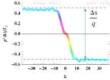
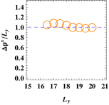
Figure 4: Intrinsic dipole moment density near the interface. (Left) Dipole moment density obtained by $p^{x}(k)/L_{y}=-e\int^{k}_{0}p\ell^{2}[\langle n_{p}\rangle-\nu]\frac{dp}{2\pi}$ (in unit of $(-e/4\pi)$). The blue dashed lines show predicted guiding-center spin $\frac{s}{q}=\frac{1}{2}(-\frac{1}{2})$ for the Pf (APf) state. The system size is $L_{y}=19\ell$. (Right) The dipole moment density across the interface $\Delta p^{x}/L_{y}$ on various cylinder width $L_{y}$. The dashed line denotes the theoretical prediction $\Delta p^{x}/L_{y}=\frac{s^{\textrm{Pf}}}{q}-\frac{s^{\textrm{APf}}}{q}=1$.

Summary and discussion.— We have presented compelling evidences that the interface between the Pfaffian (Pf) and anti-Pfaffian (APf) state has intrinsic topological properties. We identify an inhomogeneous charge distribution around the interface, where an excess of electron(hole)-like chargers is pinned to the Pf (APf) side, while the charge neutrality still holds on average. In particular, the characteristic charge profile yields an electric dipole at the interface, which is to counterbalance the mismatch in guiding-center Hall viscosity of the Pf and APf state.

Our results unveil a notable effect on the Pf-APf interface, which is overlooked in the previous discussions Wang et al. (2018); Mross et al. (2018); Lian and Wang (2018); Wan and Yang (2016). This finding may shed lights on the stability of mesoscopic puddles made of Pf and APf order (see supple ). In addition, the current work opens up a number of directions deserving further exploration. For example, it is an outstanding issue to characterize the topological nature of neutral chiral modes on the interface. Numerical studies may also further reveal rich physics of the interface made of other exotic non-Abelian states.

Acknowledgements.— W.Z. thanks Bo Yang, Jie Wang, Zhao Liu, Chong Wang, Liangdong Hu for helpful discussion. W.Z. is supported by project 11974288 from NSFC and the foundation from Westlake University. D.N.S. was supported by the U.S. Department of Energy, Office of Basic Energy Sciences under Grant No. DE-FG02-06ER46305. K.Y.’s work was supported by the National Science Foundation Grant No. DMR-1932796, and performed at the National High Magnetic Field Laboratory, which is supported by National Science Foundation Cooperative Agreement No. DMR-1644779, and the State of Florida.

In this supplemental material, we provide more details of the calculation and results to support the discussion in the main text. In Sec. A, we briefly introduce the effective edge theories that is discussed in the main text. In Sec. B, we summarize the numerical details of the infinite-size and finite-size density-matrix renormalization group (DMRG) algorithm on the cylinder geometry. This section includes four subsections. In Sec. C, we apply the same calculation method on a particle-hole symmetric state, and show a different picture from the results shown in the main text. In Sec. D, we discuss the stability of the Pfaffian-anti-Pfaffian domain wall based on our simulations. This section includes three subsections. In Sec. E, we present an analysis of edge excitations via entanglement spectra.

Appendix A A. Effective Edge Theories

In this section, we analyze the effective edge theory of the Pf-APf interface created on the cylinder geometry as shown in the main text (Fig. 2). As shown in Fig. S1, we first obtain a uniform ground state of the Pf state on an infinite long cylinder. Then we consider the following process step by step. (The analysis procedure is also shown in Fig. S1.)

1. We make an entanglement cut and bipartition the cylinder into two halves. At each side, the edge theory is described by $L^{\textrm{left}}=L_{c,+}[\phi_{e/2}]+L_{n,+}[\chi]$ and $L^{\textrm{right}}=L_{c,-}[\phi_{e/2}]+L_{n,-}[\chi]$, where $L_{x,\pm}$ describes the charged boson mode ($x=c$) (labeled by orange solid line) and the neutral fermion mode ($x=n$) (labeled by black dashed line), and $\pm$ relates to the upstream/downstream mode. If we glue the left and right part back, counter-propagating modes are all gapped out and no net edge mode appears near the interface, thus recovering the uniform gapped state in the bulk. Here the charge boson carries chiral central charge $c=1$, and neutral fermion carries $c=1/2$.

2. We perform a particle-hole operation on the right half of the cylinder, and produce a APf state on the right part. The particle-hole conjugation demands reversing the direction of all edge modes and adding another upstream integer edge mode (labeled by purple double solid line): $L^{\textrm{right}}=L_{c,-}[\phi_{e}]+L_{c,+}[\phi_{e/2}]+L_{n,+}[\chi]$. If the particle tunnel process is irrelevant, the Pf-APf interface hosts two sets of gapless edge modes, and they are placed on the left and right sides of the interface, respectively.

3. If we consider the particle tunnel process across the interface, the two charge$-e/2$ boson modes would generate a combination, and produce a downstream charge$-e$ boson mode and a boson neutral mode (labeled red wave line): $L^{\textrm{Pf-APf}}=L^{\textrm{left}}+L^{\textrm{right}}=L_{c,-}[\phi_{e}]+L_{c,+}[\phi_{e}]+L_{n,+}[\phi_{n}]+\sum_{i=1,2}L_{n,+}[\chi_{i}]$

4. The back-scattering would gapped out two couter-propagating charge modes (double solid lines), and leave the neutral modes alone on the interface: $L^{\textrm{Pf-APf}}=L_{n,+}[\phi_{n}]+\sum_{i=1,2}L_{n,+}[\chi_{i}]$ .

5. If there is emergent symmetry, one can redefine the chiral neutral boson mode as two chiral Majorana fermion modes. The neutral Majorana fermions co-propagate and thus cannot be gapped out. Consequently, the Pf-APf interface is described by four co-propagating Majorana modes： $L^{\textrm{Pf-APf}}=\sum_{i=1,2,3,4}L_{n,+}[\chi_{i}]$.

The above analysis is in line with the effective theory of Pf-APf stripe state Wan and Yang (2016). In the main text, we just present the edge structure before and after the charged modes are gapped out. The entanglement entropy provides a way to distinguish if the tunneling process is irrelevant.

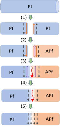
Figure S1: Microscopic edge modes at the interface. (1) Starting from the uniform Pf ground state, we make an entanglement cut and bipartition the Pf state into two halves. (2) We perform a particle-hole conjugation on the right half, and thus create the Pf-APf interface. (3) By introducing the particle tunneling across the interface, the edge reconstruction occurs. (4) Gapping out the counter-propagating charged modes leads to two co-propagating neutral Majorana modes and one neutral boson mode. (5) If further assuming the SO(4) symmetry, the resulting edge theory can be also expressed by four co-propagating neutral Majorana modes. Here black dashed lines represent the neutral chiral Majorana modes, solid orange lines represent charge$-e/2$ chiral boson modes, and double solid line is a charge$-e$ chiral boson.

Appendix B B. Details of the Computational Methods

In this section, we discuss the details about the numerical simulation.

B.1 1. Model and Hamiltonian

We discuss the single electron physics first. In the cylinder geometry, The coordinate $y$ is along the periodic direction of circumference $L_{y}$, and $x$ is along cylinder axis direction. We choose the Landau gauge $\vec{A}=(0,Bx)$ that conserves the momentum around the circumference of cylinder. In this case, each single electron orbital is labeled by an integer $m$, with a momenta $k_{m}$:

$$\psi^{N}_{m}(x,y)=\left(\frac{1}{2^{N}N!\pi^{1/2}L_{y}\ell}\right)^{1/2}\exp[i\frac{X_{m}}{\ell^{2}}y-\frac{(X_{m}-x)^{2}}{2\ell^{2}}]H_{N}(\frac{X_{m}-x}{\ell})$$ (3)

where $X_{m}=k_{m}\ell^{2}=\frac{2\pi\ell^{2}}{L_{y}}m$ is the center along x axis and $\ell$ is the magnetic length. $H_{N}(x)$ is the Hermite polynomial and N is Landau level index.

If we project into the second Landau level (setting $N=1$), the second quantization form of Hamiltonian can be expressed by

$$\hat{H} = \sum_{\{m_{i}\}}V_{m_{1},m_{2},m_{3},m_{4}}\hat{a}^{\dagger}_{m_{1}}\hat{a}^{\dagger}_{m_{2}}\hat{a}_{m_{3}}\hat{a}_{m_{4}},$$ (4)

where $V_{m_{1},m_{2},m_{3},m_{4}}$ is the interaction matrix element :

$$V_{m_{1},...,m_{4}}=\frac{1}{2L_{y}}\int^{\infty}_{-\infty}dq_{x}\sum\limits_{q_{y}=\frac{2\pi t}{L_{y}}}F_{N}(q)V(q_{x},q_{y})e^{-\frac{(q^{2}_{x}+q^{2}_{y})\ell^{2}}{2}+iq_{x}(m_{1}-m_{3})\frac{2\pi\ell^{2}}{L_{y}}}\delta_{m_{1}-m_{4},t}\delta_{m_{1}+m_{2},m_{3}+m_{4}}.$$ (5)

$F_{N}(q)=L_{N}(\frac{q^{2}\ell^{2}}{2})$ is the form factor of N-th Landau level. The function of $V(q_{x},q_{y})$ is the Fourier transformation of interaction potential $V(r)$. In this work, we choose the form of interaction as the modified Coulomb interaction

$$V(|\textbf{r}_{1}-\textbf{r}_{2}|)=\frac{1}{|\textbf{r}_{1}-\textbf{r}_{2}|}e^{-\frac{(\textbf{r}_{1}-\textbf{r}_{2})^{2}}{\xi^{2}}}.$$ (6)

Here $\xi$ is a regulated length to remove the Coulomb singularity. It has been carefully checked that, the modified Coulomb interaction can faithfully capture the essence of physics in fractional quantum Hall systems Zaletel et al. (2015a) (The different choose of $\xi$ doesnot change the physics qualitatively). In this paper, we will use this modified Coulomb interaction.

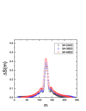
Figure S2: The entanglement entropy $\Delta S=S-S^{\textrm{Pf(APf)}}$ dependence on bipartition position $m$. Finite size effect on the domain wall structure obtained by different bond dimensions: $D=2400,3600,4800$. Physical measurements show little dependence on the bond dimensions. The system size is set to be $L_{y}=18\ell$.

B.2 2. DMRG calculations

Previously, people thought that the cylinder geometry was not suitable for the calculation of Eq. 4. The reason is, in the traditional DMRG calculation, to avoid the electrons trapped at the two ends of the finite cylinder, it is necessary to include an additional one-body potential $U(x)$. This one-body potential is un-controlled, and its selection is usually empirical. This issue can be safely overcome by using DMRG on the infinite cylinder geometry Zaletel et al. (2013). In infinite DMRG algorithm, one can access the actual results near the center by sweeping, and the edge effect should be suppressed when the length of the cylinder grows long enough (infinite long limit). So far, the infinite DMRG has been successfully applied to various FQH states ranging from Abelian states to non-Abelian states Zaletel et al. (2013, 2015b); Zhu et al. (2015).

In this work, to study the domain wall between the Pf and APf state, we combine the finite DMRG and infinite DMRG algorithm. At the first step, we perform infinite DMRG to get the Pf (APf) ground state. In all calculations, we do not presume any empirical knowledge from the model wave function. We reach the same conclusion from a random initial state or an orbital configuration according to the root configuration in the initial DMRG process. We find that, on the extensive systems with $L_{y}\in[16,24]$, the DMRG calculation will automatically select one of the Pf and APf state. Once the ground state has been fully developed, we stop the infinite growth of cylinder, and go to the finite DMRG algorithm. At the second step, we glue the Pf state and the APf state together and create a Pf-APf junction (see Fig. 1 in the main text). We fix the left (right) boundary state as the Pf (APf) state, and perform the finite DMRG variational process in the central $L_{M}$ orbitals. $L_{M}$ changes from $96$ to $234$ in this work to ensure a converged result for the interface.

In the implementation, we kept all Coulomb interaction terms $|V_{m_{1},m_{2},m_{3},m_{4}}|>10^{-6}$ within the truncated range $|m_{1}-m_{2}|<4\xi,|m_{2}-m_{3}|<\xi L_{y}/2$. We have checked that the physical quantities remain qualitatively unchanged when the truncation range is varied. In the calculations, we used the bond dimension kept up to $D=6000$. We notice that the convergence of the domain wall on $L_{y}>20$ systems is quite slow, so that we only present the results with $L_{y}\leq 20$.

B.3 3. Numerical Identification of the Pf (APf) state

The Pf (APf) state can be identified by its distinct edge spectrum. Here we analyze the degeneracy pattern of the edge excitation spectrum of the Pf state from the effective edge Hamiltonian. The edge excitation of the Pf state contains one branch of free bosons and one branch of Majorana fermions (see Appendix Sec. A), which can be described by the Hamiltonian Keski-Vakkuri and Wen (1993): $H_{\textrm{edge}}=\sum_{m>0}[E_{b}(m)b_{m}^{\dagger}b_{m}+E_{f}(m-1/2)c_{m-1/2}^{\dagger}c_{m-1/2}]$, where $b$ and $b^{\dagger}$ ($c$ and $c^{\dagger}$) are standard boson (fermion) creation and annihilation operators, and the total momentum operator is defined as $K=\sum_{m>0}[mb_{m}^{\dagger}b_{m}+(m-1/2)c_{m-1/2}^{\dagger}c_{m-1/2}]$. For even number of fermions, the edge Hamiltonian leads to a typical edge excitation spectra with counting $1,1,3,5,\cdots$ at momentum point $\Delta K=0,1,2,3,\cdots$. Here $\Delta K$ is defined as $K-K_{0}$ where $K_{0}$ is the lowest momentum ($K_{0}=0$ for even $F$).

In our calculation, the Pf (APf) state is identified by the appearance of the typical edge excitation which can be viewed from the entanglement spectra. As we discussed in Fig. 1 in the main text, the typical entanglement spectra $1,1,3,5,...$ (in the particle counting) gives the evidence of the Pf state, which relates to the root configuration $...01100110....$. Similarly, the entanglement spectra $1,1,3,5,...$ (in the hole counting) signals the APf state. The Pf and APf state has the same counting, but opposite chirality.

In addition, it is known that there are three different topological sectors for the Pf (APf) state: Identity I, neutral fermion f, and Ising anyon $\sigma$. In this paper, we focus on the identity topological sector (I) which relates to the root configuration $...01100110....$ with the edge excitation spectrum $1,1,3,5,...$ (as we discussed above). We construct the interface based on the identity sector of the Pf and APf state. In principle, one can construct the Pf-APf interface using different topological sectors. However, the emergent of quasiparticles near the interface may make the interpretation more complex. This is out of the current scope, and we will leave it for the future study.

B.4 4. More Numerical Details

In the DMRG simulation, the bond dimension parameter $D$ determines the complexity of each matrix product tensor in the calculation, therefore controls the overall accuracy in the calculations. The truncation of finite bond dimension is one source of finite size effects in our computations. So multiple values of bond dimension and its possible extrapolation to infinity is a normal scheme to check the physics in the thermodynamic limit for the given cylinder geometry. In Fig. S2, we compare the key measurements, entanglement entropy profile around the interface, for various bond dimensions. It is evident that, the domain wall structure is quite robust, which is independent of the simulation parameters. Thus, we reach the conclusion that the observed domain wall structure is intrinsic.

In addition to the bond dimension, the results on different system sizes are helpful to infer the physics in the two dimensional limit. In Fig. S3, we show the charge profiles near the Pf-APf interface for different cylinder width $L_{y}=18,19,20$. We see that,a profound domain wall structure can be identified (as we discussed in the main text), and the domain wall structure largely keeps the similar shape. In this context, we conclude that the domain wall structure that we reported here, is quite robust against the finite size effects.

Furthermore, through the comparison in Fig. S3, we notice that the charge fluctuation becomes larger in the larger system sizes. For example, on the $L_{y}=20$ cylinder, it displays ripples in a wider spatial region. This indicates that, the convergence of the domain wall on larger system sizes is quite slow, which leads to much heavier computations on larger systems. So in this work we only present the results on system sizes $L_{y}\leq 20$.

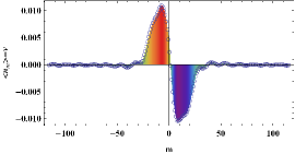
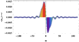
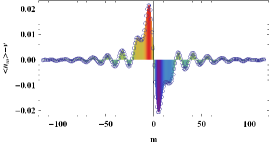
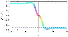
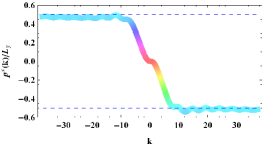
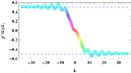
Figure S3: (Top) The charge profile near the Pf-APf interface obtained on various system sizes: $L_{y}=18$(left), 19(middle), 20 (right). $m$ denotes the Landau orbital position. The interface is at the position $m=0$. The leftmost (rightmost) side $m\rightarrow-\infty$ ($m\rightarrow\infty$) is the Pf (APf) state. (Bottom) The dipole moment density obtained by $p^{x}(k)/L_{y}$ (in unit of $(-e/4\pi)$) for $L_{y}=18$(left), 19(middle), 20 (right). The momentum is defined by $k=2\pi m/L_{y}$. The blue dashed lines show predicted guiding-center spin $\frac{s}{q}=\frac{1}{2}(-\frac{1}{2})$ for the Pf (APf) state. The bond dimension is set to be $D=2400$.

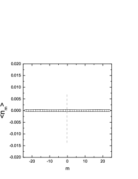
Figure S4: The charge profile of a particle-hole symmetric state after a particle-hole conjugation is applied on the left half. Here we first prepare a particle-hole symmetric state as the ground state first. We make a cut and bipartition the ground state into two halves, and then apply a particle-hole conjugation operation on the left half part (leave the right part unchanged). After the DMRG variational process, we measure the charge distribution around the gluing position $m=0$ (marked by the dashed line). The particle-hole conjugation process is the same as that in the main text.

Appendix C C. Comparison with Particle-hole symmetric state

In the main text, we elucidate that an electric dipole moment is formed to balance the Hall viscosity difference on the Pf-APf interface. To further strengthen this point, in this section we study a specific case with no Hall viscosity difference across an interface. As we show below, no dipole moment forms, if Hall viscosity difference across an interface is zero.

To be specific, we will work on the composite fermion liquid at the half filled $N=0$ Landau level, which has been proved to be particle-hole symmetric Son (2015); Geraedts et al. (2016). Following the scheme shown in the main text, we make a cut and bipartition the ground state into two halves, and then apply a particle-hole conjugation operation on the left half part of the composite fermion liquid, and leave the right part unchanged. Then we fix the boundary part and make an energy variational calculation in the central part. The obtained charge profile is shown in Fig. S4. We didnot observe charge inhomogeneity or electric domain wall structure at the gluing position (between orbital $m=-1$ and $m=0$), which is in sharp contrast to the case discussed in the main text. The understanding is straight forward: Since the composite fermion liquid is particle-hole symmetric and its guiding center spin takes $\frac{s}{q}=0$, no viscosity force is generated thus no electric dipole moment should appear. In a word, through this test, we further strengthen that, the formation of electric dipole moment on the Pf-APf interface is intrinsic to the mismatch of the Hall viscosity (guiding-center spin) of the two distinct topological orders (as we emphasize in the main text).

Appendix D D. Stability of the Domain Wall: Implications on the random puddles picture

In this section, we discuss the stability of the Pf-APf domain wall. We address whether or not it is mechanically or energetically favored in the experimental condition, from the view of numerical simulations.

D.1 1. Spatial size of the Domain wall

As discussed in the main text, the domain wall on the interface has a spatial length scale, $d=d_{\textrm{Pf}}+d_{\textrm{APf}}$, which describes the distance that domain wall penetrates into the Pf (APf) side (see Fig. 3 in the main text). In our extensive calculation, we estimate this length scale is largely around $d\gtrsim 16\ell$ ($\ell$ is the magnetic length), depending on the system size $L_{y}$. If we take the magnetic length as $\ell=7.9$nm for external magnetic field strength $B=10$T, we have the length scale $d\gtrsim 126$nm. To connect this estimation to the theoretical proposal in Ref. Wang et al. (2018); Lian and Wang (2018), where a particle-hole symmetric state is realized by random puddles made of Pf and aPf domains, we assume each puddle has minimal size $\sim 4d$ ($\sim 2d$ length for boundary and $>2d$ length for separation between two boundary). Then we estimate the minimal size of a puddle made of the Pf and APf state is $\gtrsim 4d\sim 504$nm (for $B=10$T).

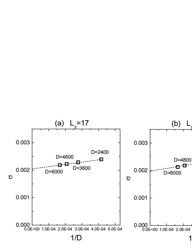
Figure S5: The tension $\sigma$ (in unit of $e^{2}/\ell^{2}$) of a domain wall at the Pf-APf interface, obtained on various bond dimension: $D=2400,3600,4800,6000$. By extrapolating $\sigma$ using a linear function of $D^{-1}$ gives the estimation in $D\rightarrow\infty$.

D.2 2. Energetics of the Domain wall

In our setup (see discussion in Fig. 1 in the main text), the ground state energy of the Pf (APf) state on the infinite long cylinder is expressed as

$$E^{\textrm{Pf}} =L^{\textrm{Pf}}+C^{\textrm{Pf}}+R^{\textrm{Pf}},$$ (7)

$$E^{\textrm{APf}} =L^{\textrm{APf}}+C^{\textrm{APf}}+R^{\textrm{APf}},$$ (8)

where $L^{\textrm{Pf(APf)}}$ ($R^{\textrm{Pf(APf)}}$) is the energy of the leftmost (rightmost) boundary for the Pf (APf) state, and $C^{\textrm{Pf(APf)}}$ describes the energy from the central part enclosing $L_{M}$ orbitals.

Next we consider the Pf-APf domain wall (see Fig. 1 in the main text), sandwiched between a Pf state (on the leftmost side) and a APf state (on the rightmost side). The obtained energy of this whole system is $E^{\textrm{Pf-APf}}$, which contains three parts:

$$E^{\textrm{Pf-APf}}=L^{\textrm{Pf}}+C^{\textrm{domain}}+R^{\textrm{APf}}.$$ (9)

Then the energy of domain wall can be derived as

$$C^{\textrm{domain}}=E^{\textrm{Pf-APf}}-(L^{\textrm{Pf}}+R^{\textrm{APf}})=E^{\textrm{Pf-APf}}-\frac{1}{2}[(E^{\textrm{Pf}}+E^{\textrm{APf}})-(C^{\textrm{Pf}}+C^{\textrm{APf}})].$$ (10)

Therefore, the energy cost of domain wall $\delta=\sigma L_{y}$ compared to the uniform Pf (APf) state is

$$\delta=\sigma\cdot L_{y}=C^{\textrm{domain}}-\frac{1}{2}(C^{\textrm{Pf}}+C^{\textrm{APf}})=E^{\textrm{Pf-APf}}-\frac{1}{2}(E^{\textrm{Pf}}+E^{\textrm{APf}})$$ (11)

where $\sigma$ is the domain wall tension.

First of all, in our extensive calculations, the obtained domain wall energy cost $\delta$ are all positive (in our extensive tests, on all system sizes and calculation parameters, the domain wall energy costs are positive). That means, one need to take finite energy cost to (potentially) excite a Pf-APf domain wall structure. It indicates the formation of Pf-APf domain wall structure is less favored as the ground state (in the translational invariant system), compared with the Pf or APf state (in a translational invariant system). (It is further supported by that, we didnot observe any tendency in our DMRG calculation that the ground state is non-uniform.) That is, the other mechanism (e.g. disorder, random potentials) should play some role in stabilizing and favoring a Pf-APf puddles Mross et al. (2018); Wang et al. (2018); Lian and Wang (2018) (also see discussion below).

In Fig. S5, we compute the domain wall tension $\sigma$, for a typical cylinder width $L_{y}=18\ell,19\ell,20\ell$. We also extrapolate the calculated results using the $D^{-1}$ ($D$ is bond dimension). In Tab. S1, we list the obtained domain wall tension on various system sizes. In a rough estimation, the domain wall tension is around $\sigma\in[0.0017,0.0021]$ (in unit of $e^{2}/\ell^{2}$). The order of this domain wall tension is largely consistent with the recent work Simon et al. (2020).

Table S1: Estimated domain wall energy and tension on different system sizes.

$L_{y}(\ell)$	$17.0$	$17.5$	$18.0$	$18.5$	$19.0$	$19.5$
$\delta(e^{2}/\ell)$	$0.0349$	$0.0355$	$0.0356$	$0.03381$	$0.0358$	$0.0344$
$\sigma(e^{2}/\ell^{2})$	$0.00205$	$0.00203$	$0.00198$	$0.00183$	$0.00188$	$0.00176$

Figure S6: (top) The refined structure of the puddle made of Pf-APf domain wall. (bottom) The disorder potential could stabilize the Pf-APf puddle.

D.3 3. Stability of the Domain-wall

In Ref. Wang et al. (2018); Lian and Wang (2018); Mross et al. (2018), it has been proposed a particle-hole symmetric topological order made of domains of Pf and APf state. Here, our results imply that, if such state is possible, there is a refined structure (Fig.S6(top left)) which is overlooked in the previous discussion: The puddle hosts electric dipole moment (denoted by the blue arrow) on the interface (black line) between the Pf and APf state. The form of this dipole moment has topological origin (as discussed in the main text). Nevertheless, this puddle structure is not structurally stable, under the action of a driving force. For example, considering an external electric field, the coupling between the electric field and dipole moment requires the dipole moment tends to parallel to the direction of the electric field, thus the dipole moment structure shown in Fig. S6(top) is not stable. Next we argue that, effects of disorder could stabilize the puddle structure. As shown in the Fig. S6(bottom), we assume that disorder creates a relatively weak potential (grey dashed line). In this case, the puddle structure can be pinned to the equipotential plane of the disorder potential. The domain wall tension should be at least smaller than the confining potential provided by the disorder potential, say $\sigma\lesssim(\Delta p^{x}/L_{y})\cdot E_{dis}$ ($\Delta p^{x}/L_{y}$ is the electric dipole density as discussed in the main text). Thus we estimate that the electric field from disorder potential has the order of $E_{dis}\sim 2.9\times 10^{5}V/m$ (we take $\sigma\sim 2\times 10^{-3}e^{2}/\ell^{2}$ (see Tab.S1), $\ell=11.18$nm at $B=5T$).

At last, we compare this estimated disorder potential with the experimental conditions. In the high-mobility $GaAs/Ga_{1-x}Al_{x}As$ heterojunction, the donor layer is usually separated from the two-dimensional electron gas by a typical length scale $d\sim 100nm$. Thus we estimate the typical disorder potential in experiments as $E^{\textrm{exp}}_{dis}\approx kQ/d^{2}=(9\times 10^{9}Nm^{2}/C)\times(1.6\times 10^{-19}C)/(10^{-7}m)^{2}\approx 1.5\times 10^{-5}V/m$. Through this estimation, we find that the required disorder potential to stabilize the domain wall is largely in the same order with the current experimental condition.

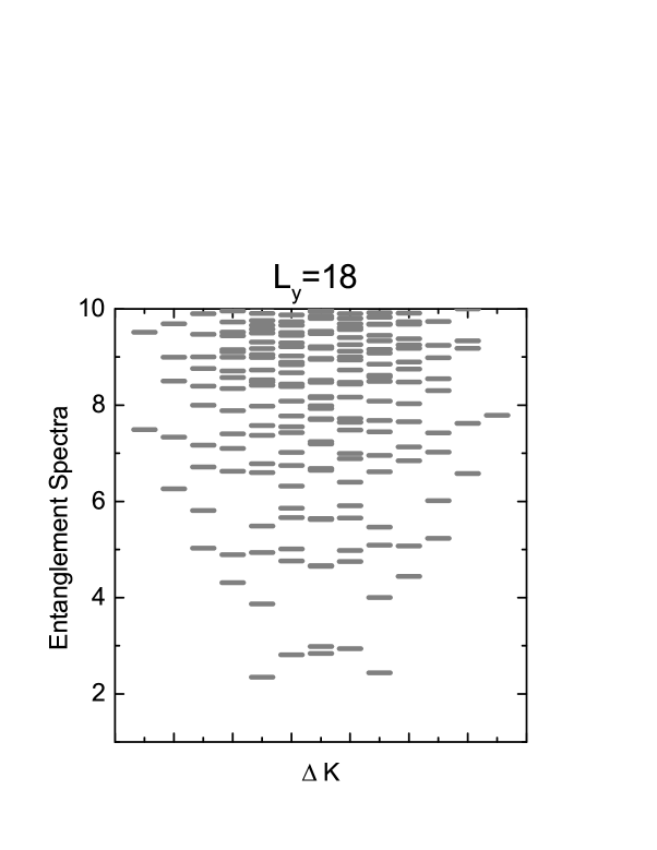
Figure S7: The entanglement spectra (the entanglement cut position is chosen at the center of Pf-APf interface) obtained on various system sizes: $L_{y}=18$(left), 19(middle), 20 (right). The bond dimension is set to be $D=2400$.

Appendix E E. Entanglement spectra

In this section, we present the entanglement spectra at the Pf-APf interface. The typical entanglement spectra at the interface is shown in Fig. S7. (The entanglement cutting position is at the center of the interface, where the entanglement entropy reaches a maximum value (as shown in Fig. 2 in the main text).) Interestingly, it is found the entanglement spectra is almost particle-hole symmetric, despite of small deviations. This could be understood, if we recall the root pattern in the thin-torus limit (see the discussion in the main text). That is, looking particle excitations from the interface of the Pf side is similar to looking hole excitations from that of the APf side.

The emergence of particle-hole symmetry at the interface provides a numerical self-consistency check of the our computation. Importantly, it shows that the center of the interface is special. Due to this emergence of particle-hole symmetry, the guiding-center spin and related guiding-center Hall viscosity at the interface should be zero. Thus we can select this point as a reference to compare the guiding-center viscosity of the Pf or APf state.

References

- Willett et al. (1987) R. Willett, J. P. Eisenstein, H. L. Störmer, D. C. Tsui, A. C. Gossard, and J. H. English, Phys. Rev. Lett. 59, 1776 (1987).
- Pan et al. (1999) W. Pan, J.-S. Xia, V. Shvarts, D. E. Adams, H. L. Stormer, D. C. Tsui, L. N. Pfeiffer, K. W. Baldwin, and K. W. West, Phys. Rev. Lett. 83, 3530 (1999).
- Pan et al. (2008) W. Pan, J. S. Xia, H. L. Stormer, D. C. Tsui, C. Vicente, E. D. Adams, N. S. Sullivan, L. N. Pfeiffer, K. W. Baldwin, and K. W. West, Phys. Rev. B 77, 075307 (2008).
- Choi et al. (2008) H. C. Choi, W. Kang, S. Das Sarma, L. N. Pfeiffer, and K. W. West, Phys. Rev. B 77, 081301 (2008).
- Dolev et al. (2008) M. Dolev, M. Heiblum, V. Umansky, A. Stern, and D. Mahalu, Nature 452, 529 (2008).
- Radu et al. (2008) I. P. Radu, J. B. Miller, C. M. Marcus, M. A. Kastner, L. N. Pfeiffer, and K. W. West, Science 320, 899 (2008).
- Bid et al. (2010) A. Bid, N. N. Ofek, H. Inoue, M. Heiblum, C. L. Kane, V. Umansky, and D. D. Mahalu, Nature 466, 585 (2010).
- Willett et al. (2013) R. L. Willett, C. Nayak, K. Shtengel, L. N. Pfeiffer, and K. W. West, Phys. Rev. Lett. 111, 186401 (2013).
- Stern et al. (2010) M. Stern, P. Plochocka, V. Umansky, D. K. Maude, M. Potemski, and I. Bar-Joseph, Phys. Rev. Lett. 105, 096801 (2010).
- Tiemann et al. (2012) L. Tiemann, G. Gamez, N. Kumada, and K. Muraki, Science 335, 828 (2012).
- Baer et al. (2014) S. Baer, C. Rössler, T. Ihn, K. Ensslin, C. Reichl, and W. Wegscheider, Phys. Rev. B 90, 075403 (2014).
- Venkatachalam et al. (2011) V. Venkatachalam, A. Yacoby, L. Pfeiffer, and K. West, Nature 469, 185 (2011).
- Kitaev (2003) A. Kitaev, Annals of Physics 303, 2 (2003).
- Nayak et al. (2008) C. Nayak, S. H. Simon, A. Stern, M. Freedman, and S. Das Sarma, Rev. Mod. Phys. 80, 1083 (2008).
- Moore and Read (1991) G. Moore and N. Read, Nuclear Physics B 360, 362 (1991).
- Greiter et al. (1991) M. Greiter, X.-G. Wen, and F. Wilczek, Phys. Rev. Lett. 66, 3205 (1991).
- Read and Green (2000) N. Read and D. Green, Phys. Rev. B 61, 10267 (2000).
- Morf (1998) R. H. Morf, Phys. Rev. Lett. 80, 1505 (1998).
- Rezayi and Haldane (2000) E. H. Rezayi and F. D. M. Haldane, Phys. Rev. Lett. 84, 4685 (2000).
- Wan et al. (2006) X. Wan, K. Yang, and E. H. Rezayi, Phys. Rev. Lett. 97, 256804 (2006).
- Hu et al. (2009) Z.-X. Hu, E. H. Rezayi, X. Wan, and K. Yang, Phys. Rev. B 80, 235330 (2009).
- Möller and Simon (2008) G. Möller and S. H. Simon, Phys. Rev. B 77, 075319 (2008).
- Peterson et al. (2008) M. R. Peterson, T. Jolicoeur, and S. Das Sarma, Phys. Rev. Lett. 101, 016807 (2008).
- Wang et al. (2009) H. Wang, D. N. Sheng, and F. D. M. Haldane, Phys. Rev. B 80, 241311 (2009).
- Wójs et al. (2010) A. Wójs, C. Tőke, and J. K. Jain, Phys. Rev. Lett. 105, 096802 (2010).
- Storni et al. (2010) M. Storni, R. H. Morf, and S. Das Sarma, Phys. Rev. Lett. 104, 076803 (2010).
- Feiguin et al. (2008) A. E. Feiguin, E. Rezayi, C. Nayak, and S. Das Sarma, Phys. Rev. Lett. 100, 166803 (2008).
- Storni and Morf (2011) M. Storni and R. H. Morf, Phys. Rev. B 83, 195306 (2011).
- Pakrouski et al. (2015) K. Pakrouski, M. R. Peterson, T. Jolicoeur, V. W. Scarola, C. Nayak, and M. Troyer, Phys. Rev. X 5, 021004 (2015).
- Zhu et al. (2016) W. Zhu, Z. Liu, F. D. M. Haldane, and D. N. Sheng, Phys. Rev. B 94, 245147 (2016).
- Levin et al. (2007) M. Levin, B. I. Halperin, and B. Rosenow, Phys. Rev. Lett. 99, 236806 (2007).
- Lee et al. (2007) S.-S. Lee, S. Ryu, C. Nayak, and M. P. A. Fisher, Phys. Rev. Lett. 99, 236807 (2007).
- Zaletel et al. (2015a) M. P. Zaletel, R. S. K. Mong, F. Pollmann, and E. H. Rezayi, Phys. Rev. B 91, 045115 (2015a).
- Rezayi (2017) E. H. Rezayi, Phys. Rev. Lett. 119, 026801 (2017).
- Banerjee et al. (2018) M. Banerjee, M. Heiblum, V. Umansky, D. E. Feldman, Y. Oreg, and A. Stern, Nature 559, 205 (2018).
- Zucker and Feldman (2016) P. T. Zucker and D. E. Feldman, Phys. Rev. Lett. 117, 096802 (2016).
- Chen et al. (2014) X. Chen, L. Fidkowski, and A. Vishwanath, Phys. Rev. B 89, 165132 (2014).
- Simon (2018a) S. H. Simon, Phys. Rev. B 97, 121406 (2018a).
- Feldman (2018) D. E. Feldman, Phys. Rev. B 98, 167401 (2018).
- Simon (2018b) S. H. Simon, Phys. Rev. B 98, 167402 (2018b).
- Mross et al. (2018) D. F. Mross, Y. Oreg, A. Stern, G. Margalit, and M. Heiblum, Phys. Rev. Lett. 121, 026801 (2018).
- Wang et al. (2018) C. Wang, A. Vishwanath, and B. I. Halperin, Phys. Rev. B 98, 045112 (2018).
- Lian and Wang (2018) B. Lian and J. Wang, Phys. Rev. B 97, 165124 (2018).
- Wan and Yang (2016) X. Wan and K. Yang, Phys. Rev. B 93, 201303 (2016).
- Wen (2004) X.-G. Wen, “Quantum field theory of many-body systems: from the origin of sound to an origin of light and electrons,” (2004).
- Keski-Vakkuri and Wen (1993) E. Keski-Vakkuri and X.-G. Wen, International Journal of Modern Physics B 7, 4227 (1993).
- Li and Haldane (2008) H. Li and F. D. M. Haldane, Phys. Rev. Lett. 101, 010504 (2008).
- Qi et al. (2012) X.-L. Qi, H. Katsura, and A. W. W. Ludwig, Phys. Rev. Lett. 108, 196402 (2012).
- Das Sarma et al. (2005) S. Das Sarma, M. Freedman, and C. Nayak, Phys. Rev. Lett. 94, 166802 (2005).
- Stern and Halperin (2006) A. Stern and B. I. Halperin, Phys. Rev. Lett. 96, 016802 (2006).
- Bonderson et al. (2006) P. Bonderson, A. Kitaev, and K. Shtengel, Phys. Rev. Lett. 96, 016803 (2006).
- Fendley et al. (2006) P. Fendley, M. P. A. Fisher, and C. Nayak, Phys. Rev. Lett. 97, 036801 (2006).
- Milovanović and Read (1996) M. Milovanović and N. Read, Phys. Rev. B 53, 13559 (1996).
- Sandler et al. (1998) N. P. Sandler, C. d. C. Chamon, and E. Fradkin, Phys. Rev. B 57, 12324 (1998).
- Kapustin and Saulina (2011) A. Kapustin and N. Saulina, Nuclear Physics B 845, 393–435 (2011).
- Kitaev and Kong (2012) A. Kitaev and L. Kong, Communications in Mathematical Physics 313, 351–373 (2012).
- Barkeshli et al. (2013) M. Barkeshli, C.-M. Jian, and X.-L. Qi, Phys. Rev. B 88, 241103 (2013).
- Levin (2013) M. Levin, Phys. Rev. X 3, 021009 (2013).
- Lu and Lee (2014) Y.-M. Lu and D.-H. Lee, Phys. Rev. B 89, 205117 (2014).
- Cano et al. (2015) J. Cano, M. Cheng, M. Barkeshli, D. J. Clarke, and C. Nayak, Phys. Rev. B 92, 195152 (2015).
- Yang (2017) K. Yang, Phys. Rev. B 96, 241305 (2017).
- Santos et al. (2018) L. H. Santos, J. Cano, M. Mulligan, and T. L. Hughes, Phys. Rev. B 98, 075131 (2018).
- Crépel et al. (2019a) V. Crépel, N. Claussen, N. Regnault, and B. Estienne, Nat. Comm. 10, 1860 (2019a).
- Crépel et al. (2019b) V. Crépel, N. Claussen, B. Estienne, and N. Regnault, Nat. Comm. 10, 1861 (2019b).
- Jaworowski and Nielsen (2019) B. Jaworowski and A. E. B. Nielsen, “Model wavefunctions for interfaces between lattice laughlin states,” (2019), arXiv:1911.12380 [cond-mat.str-el] .
- Grosfeld and Schoutens (2009) E. Grosfeld and K. Schoutens, Phys. Rev. Lett. 103, 076803 (2009).
- Bais et al. (2009) F. A. Bais, J. K. Slingerland, and S. M. Haaker, Phys. Rev. Lett. 102, 220403 (2009).
- Barkeshli et al. (2015) M. Barkeshli, M. Mulligan, and M. P. A. Fisher, Phys. Rev. B 92, 165125 (2015).
- Chamon and Wen (1994) C. d. C. Chamon and X. G. Wen, Phys. Rev. B 49, 8227 (1994).
- Wan et al. (2002) X. Wan, K. Yang, and E. H. Rezayi, Phys. Rev. Lett. 88, 056802 (2002).
- Wan et al. (2003) X. Wan, E. H. Rezayi, and K. Yang, Phys. Rev. B 68, 125307 (2003).
- (72) See Supplemental Material.
- Zaletel et al. (2015b) M. P. Zaletel, R. S. K. Mong, F. Pollmann, and E. H. Rezayi, Phys. Rev. B 91, 045115 (2015b).
- White (1992) S. R. White, Phys. Rev. Lett. 69, 2863 (1992).
- McCulloch (2008) I. P. McCulloch, arXiv e-prints , arXiv:0804.2509 (2008), arXiv:0804.2509 [cond-mat.str-el] .
- Zaletel et al. (2013) M. P. Zaletel, R. S. K. Mong, and F. Pollmann, Phys. Rev. Lett. 110, 236801 (2013).
- Zhu et al. (2015) W. Zhu, S. S. Gong, F. D. M. Haldane, and D. N. Sheng, Phys. Rev. Lett. 115, 126805 (2015).
- Wen and Zee (1992) X. G. Wen and A. Zee, Phys. Rev. Lett. 69, 953 (1992).
- Wu et al. (2014) Y.-L. Wu, B. Estienne, N. Regnault, and B. A. Bernevig, Phys. Rev. Lett. 113, 116801 (2014).
- Bergholtz and Karlhede (2005) E. J. Bergholtz and A. Karlhede, Phys. Rev. Lett. 94, 026802 (2005).
- Bernevig and Haldane (2008) B. A. Bernevig and F. D. M. Haldane, Phys. Rev. Lett. 100, 246802 (2008).
- Avron et al. (1995) J. E. Avron, R. Seiler, and P. G. Zograf, Phys. Rev. Lett. 75, 697 (1995).
- Haldane (2009) F. Haldane, arXiv preprint arXiv:0906.1854 (2009).
- Haldane (2011) F. D. M. Haldane, Phys. Rev. Lett. 107, 116801 (2011).
- Read (2009) N. Read, Phys. Rev. B 79, 045308 (2009).
- Read and Rezayi (2011) N. Read and E. H. Rezayi, Phys. Rev. B 84, 085316 (2011).
- Park and Haldane (2014) Y. Park and F. D. M. Haldane, Phys. Rev. B 90, 045123 (2014).
- Zhu and Sheng (2019) W. Zhu and D. N. Sheng, Phys. Rev. Lett. 123, 056804 (2019).
- Simon et al. (2020) S. H. Simon, M. Ippoliti, M. P. Zaletel, and E. H. Rezayi, Phys. Rev. B 101, 041302 (2020).
- Son (2015) D. T. Son, Phys. Rev. X 5, 031027 (2015).
- Geraedts et al. (2016) S. D. Geraedts, M. P. Zaletel, R. S. K. Mong, M. A. Metlitski, A. Vishwanath, and O. I. Motrunich, Science 352, 197–201 (2016).