Extended Cuscuton as Dark Energy

Abstract

Late-time cosmology in the extended cuscuton theory is studied, in which gravity is modified while one still has no extra dynamical degrees of freedom other than two tensor modes. We present a simple example admitting analytic solutions for the cosmological background evolution that mimics $\Lambda$CDM cosmology. We argue that the extended cuscuton as dark energy can be constrained, like usual scalar-tensor theories, by the growth history of matter density perturbations and the time variation of Newton’s constant.

I Introduction

General relativity (GR) has been the most successful gravitational theory. It has the Newtonian and post-Newtonian limit consistent with experiments, and predicts the existence of gravitational waves and black holes, which has been directly confirmed in recent years Abbott et al. (2016); Akiyama et al. (2019). Moreover, GR with a cosmological constant can explain the present accelerated expansion of the Universe.

Due to its simplicity, the cosmological constant has been an appealing candidate for the origin of the present accelerated expansion. In order to test this paradigm, it is helpful to compare it with alternative models, i.e., dark energy/modified gravity models. A guideline for modifying GR is given by the Lovelock’s theorem Lovelock (1971). The theorem states that the most general theory in four dimensions having at most second-order Euler-Lagrange equations, respecting general covariance, and written in terms of only the metric is nothing but GR with a cosmological constant. Here, the second-order nature of field equations is desirable, since higher-order field equations generically lead to unstable extra degrees of freedom (DOFs) called Ostrogradsky ghosts Woodard (2015); Motohashi and Suyama (2020) unless the higher derivative terms are degenerate Motohashi and Suyama (2015); Langlois and Noui (2016); Motohashi et al. (2016a); Klein and Roest (2016); Motohashi et al. (2018a, b). Hence, a natural way to extend the framework of GR plus a cosmological constant is to incorporate some new DOFs on top of the metric in such a way that the action does not contain nondegenerate higher derivative interactions. To capture aspects of such dark energy/modified gravity models, it is useful to consider those having a single scalar field in addition to the metric, i.e., the class of scalar-tensor theories. Even in this restricted class, there exist innumerably many theories, so we need a comprehensive framework to treat them in a unified manner. The Horndeski theory Horndeski (1974); Deffayet et al. (2011); Kobayashi et al. (2011) is a well-known such comprehensive framework, since it is the most general scalar-tensor theory in four dimensions whose Euler-Lagrange equations are at most second-order. By allowing for the existence of degenerate higher derivative terms in the Euler-Lagrange equations, the Horndeski theory is generalized to the Gleyzes-Langlois-Piazza-Vernizzi (GLPV, also known as beyond Horndeski) theory Gleyzes et al. (2015) and further to degenerate higher-order scalar-tensor (DHOST, also known as extended scalar-tensor) theories Langlois and Noui (2016); Crisostomi et al. (2016); Ben Achour et al. (2016); Takahashi and Kobayashi (2017); Langlois et al. (2019). For recent reviews, see Langlois (2019); Kobayashi (2019).

Generically, such healthy scalar-tensor theories possess three dynamical DOFs, two of which come from the metric and one from the scalar field. However, there are some special models where only two DOFs are dynamical as in GR Lin and Mukohyama (2017); Chagoya and Tasinato (2019); Aoki et al. (2018); Afshordi et al. (2007a); Iyonaga et al. (2018); Gao and Yao (2020). In this sense, these models can be regarded as minimal modifications of GR, which could provide the second most economical explanation of the accelerated expansion next to the cosmological constant. Indeed, the authors of Aoki et al. (2019) showed that the model proposed in Aoki et al. (2018) can explain dark energy. This model was obtained by performing a canonical transformation on GR, utilizing the idea that a canonical transformation preserves the number of physical DOFs Domènech et al. (2015); Takahashi et al. (2017). Along this line, we focus on the framework Iyonaga et al. (2018) of ourselves, which was invented as an extension of the cuscuton theory Afshordi et al. (2007a). Regarding the original cuscuton model, its various aspects have been studied. A Hamiltonian analysis was performed in Gomes and Guariento (2017). The cosmic microwave background and matter power spectra can be distinguished from those in GR Afshordi et al. (2007b). Stable bounce cosmology Boruah et al. (2018); Quintin and Yoshida (2020), a reasonable power-law inflation model Ito et al. (2019a), and an accelerating universe with an extra dimension Ito et al. (2019b) based on the cuscuton have been studied. It was also shown that the cuscuton theory with a quadratic potential can be considered as a low-energy limit of the (non-projectable) Hořava-Lifshitz theory Afshordi (2009); Bhattacharyya et al. (2018). The authors of de Rham and Motohashi (2017) pointed out the absence of caustic singularities in cuscuton-like scalar field theories. Moreover, the cuscuton admits extra symmetries other than the Poincaré symmetry Pajer and Stefanyszyn (2019); Grall et al. (2020). These fascinating features of the cuscuton model motivated us to specify a broader class of scalar-tensor theories that inherit the two-DOF nature of the cuscuton, which we dubbed the “extended cuscuton.” The aim of this paper is to investigate its cosmological aspects as to whether the extended cuscuton can account for the current accelerated expansion of the Universe.

The rest of this paper is organized as follows. In §II, we briefly explain the framework of extended cuscutons and present its action. Then, in §III, we study cosmology in this class of models in the presence of a matter field. We derive the background field equations and the quadratic action for scalar perturbations. Also, we propose some requirements for the extended cuscutons to be a viable dark energy model. In §IV, we focus on an analytically solvable case and obtain criteria for the model to satisfy the viability requirements. We find that this model can mimic the cosmological background evolution in the $\Lambda$CDM model, though the dynamics of the density fluctuations in general deviates from the one in the $\Lambda$CDM case. Finally, we summarize our discussion in §V.

II The model

In Iyonaga et al. (2018), the extended cuscuton model was obtained as a class of DHOST (more precisely, GLPV) theories in which the scalar field is nondynamical. In the present paper, we focus on a subclass where the speed of gravitational waves, $c_{\rm GW}$, is equal to that of light, $c_{\rm light}(\coloneqq 1)$. This is partly for simplicity and partly because the recent simultaneous observation of the gravitational waves GW170817 and the $\gamma$-ray burst 170817A emitted from a neutron star binary showed that $c_{\rm GW}$ coincides with $c_{\rm light}$ to a precision of $10^{-15}$ at least in the low-redshift universe ($z\lesssim 0.01$) Abbott et al. (2017a, b, c); Sakstein and Jain (2017). This subclass is described by the following action:

$$S_{\rm EC}=\int d^{4}x\sqrt{-g}\left[G_{2}(\phi,X)+G_{3}(\phi,X)\Box\phi+G_{4}(\phi)R\right],$$ (1)

with

$$\begin{split}G_{2}&=u_{2}+v_{2}\sqrt{2X}-\left(2v_{3\phi}+4v_{4\phi\phi}+\frac{3v_{3}^{2}}{4v_{4}}\right)X+\left(v_{3\phi}+2v_{4\phi\phi}\right)X\log X,\\ G_{3}&=-\left(\frac{v_{3}}{2}+v_{4\phi}\right)\log X,\quad G_{4}=v_{4},\end{split}$$ (2)

where $X\coloneqq-g^{\mu\nu}\partial_{\mu}\phi\partial_{\nu}\phi/2$ and $R$ is the Ricci scalar. Also, $u_{2},v_{2},v_{3}$, and $v_{4}$ are arbitrary functions of $\phi$, and a subscript $\phi$ denotes a derivative with respect to $\phi$. Note in passing that any model described by the action (1) satisfies $c_{\rm GW}=1$ around arbitrary backgrounds even without the “cuscuton tuning” (2) since it is conformally equivalent to general relativity with a scalar field in the form of kinetic gravity braiding Deffayet et al. (2010) (see also Kobayashi et al. (2010)). The appearance of $\log X$ in the action is one of the characteristic features of the extended cuscutons, which also appears in other contexts (see Pujolàs et al. (2011); Afshordi et al. (2014) for examples). Interestingly, our model is conformally equivalent to the one in Afshordi et al. (2014). Note also that the original cuscuton model proposed in Afshordi et al. (2007a) amounts to the choice $v_{3}=0$ and $v_{4}=M_{\rm Pl}^{2}/2$.

We have three caveats on the physical DOFs of the extended cuscuton. The first is about the relation between the DOFs and the homogeneity of the scalar field. For the original cuscuton with timelike $\partial_{\mu}\phi$, the authors of Gomes and Guariento (2017) claimed that $\phi$ in general carries a scalar DOF and it vanishes only in the homogeneous limit. However, this result is counterintuitive as one can always make the scalar field homogeneous, $\phi=\phi(t)$, by choosing the coordinate system appropriately (called the unitary gauge) when $\partial_{\mu}\phi$ is timelike. We clarified this point in our previous paper Iyonaga et al. (2018) by showing that the potentially existing scalar DOF actually does not propagate if an appropriate boundary condition is imposed. Thus, provided that $\partial_{\mu}\phi$ is timelike, taking the unitary gauge does not change the number of physical DOFs, which allows us to choose this gauge in the following section.

The second is about the direction of $\partial_{\mu}\phi$. The above action applies to situations with timelike $\partial_{\mu}\phi$ (i.e., $X>0$) so that $\sqrt{2X}$ and $\log X$ are real. In order to incorporate cases with spacelike $\partial_{\mu}\phi$, one may replace $X\to|X|$. In the resultant model, one finds that the number of dynamical DOFs depends on whether $\partial_{\mu}\phi$ is timelike or spacelike Iyonaga et al. (2018). Specifically, when the gradient of the scalar field is spacelike, the scalar field remains dynamical as usual scalar-tensor theories. This is similar to what happens in the spatially covariant gravity Gao (2014) and U-degenerate theory De Felice et al. (2018), where a would-be unstable extra DOF becomes nondynamical when $\partial_{\mu}\phi$ is timelike. As such, the scalar field breaks the Lorentz invariance and only the space diffeomorphisms remain. There are many observational constraints on the Lorentz violation, e.g., from the Solar System tests Blas et al. (2011); Will (2014) and more recently from binary black hole observations Abbott et al. (2017c); Emir Gümrükçüoğlu et al. (2018); Ramos and Barausse (2019). These observational constraints should restrict our model, but it is beyond the scope of the present paper.

The third is about the existence of an extra half DOF. As established in Iyonaga et al. (2018), the model (1) is guaranteed to have less-than-three DOFs provided that the gradient of the scalar field is timelike. The authors of Gao and Yao (2020) performed a more detailed Hamiltonian analysis to show that one needs an additional condition in general to ensure the two-DOF nature, or otherwise there remains an extra half DOF. The Hořava-Lifshitz gravity is one of the theories where the extra half DOF exhibits undesired behaviors Blas et al. (2009). For instance, the mode frequency of the half DOF diverges for static or spatially homogeneous backgrounds. Also, the phase space of the Hořava-Lifshitz gravity is described by odd number of variables, which means that there is no symplectic structure. The constraint structure of our extended cuscuton is similar to the Hořava-Lifshitz gravity, so something similar might happen to our model when there is an extra half DOF. In order for the specific model (1) to have exactly two DOFs, $v_{4}$ should be a nonvanishing constant. However, we consider $\phi$-dependent $v_{4}$ in this paper, as this potentially pathological half DOF does not show up in the present cosmological setup.

III Cosmology

III.1 Background

We study a homogeneous and isotropic universe in the presence of a matter field, and hence consider the following action:

$$S=S_{\rm EC}+\int d^{4}x\sqrt{-g}\mathcal{L}_{\rm m}.$$ (3)

The metric $g_{\mu\nu}$ and cuscuton $\phi$ are assumed to have the form

$$g_{\mu\nu}dx^{\mu}dx^{\nu}=-N^{2}(t)dt^{2}+a^{2}(t)\delta_{ij}dx^{i}dx^{j},\quad\phi=\phi(t).$$ (4)

In order to mimic barotropic perfect fluid, we write the matter Lagrangian $\mathcal{L}_{\rm m}$ in terms of a scalar field $\chi$ as in Armendáriz-Picón et al. (1999),

$$\mathcal{L}_{\rm m}=P(Y),\quad Y\coloneqq-\frac{1}{2}g^{\mu\nu}\partial_{\mu}\chi\partial_{\nu}\chi.$$ (5)

Here, $\chi$ is assumed to be a function of $t$ only.Then, the energy density, pressure, and squared sound speed of $\chi$ are respectively written as

$$\rho_{\mathrm{m}}=2YP_{Y}-P,\quad p_{\mathrm{m}}=P,\quad c_{\rm s}^{2}=\frac{P_{Y}}{P_{Y}+2YP_{YY}},$$ (6)

where $P_{Y}\coloneqq dP/dY$. We substitute the ansatz (4) into the action (3), from which we can derive the field equations for $N$, $a$, $\phi$, and $\chi$. Among these EOMs, we focus on those for $N$, $a$, and $\phi$ since only three of the four EOMs are independent. Note that the EOM for $N$ cannot be reproduced from the other EOMs. Therefore, one may set $N=1$ only after deriving the EOM for $N$ Motohashi et al. (2016b). When we consider late-time cosmology where only the dust component is important, we may set $p_{\rm m}=0$ and $c_{\rm s}=0$. One may naively think that this dust limit is ill-defined in the present case where we mimic perfect-fluid matter by (5), since $p_{\rm m}\to 0$ implies $\mathcal{L}_{\rm m}=P(Y)\to 0$. Nevertheless, once we rewrite every $P$ and its derivative in terms of $\rho_{\rm m}$, $p_{\rm m}$, and $c_{\rm s}$, we can safely take the dust limit Boubekeur et al. (2008).

In deriving the field equations, we assume the time derivative of $\phi$ satisfies $\dot{\phi}>0$ to fix the branch of the square root originating from the term $\sqrt{2X}$ in (2). One could in principle assume $\dot{\phi}<0$ instead, and in that case one should replace $v_{2}\to-v_{2}$ in the following analysis. The Euler-Lagrange equations for $N$ and $a$ read, respectively,

$$\mathcal{E}_{N} \coloneqq 6v_{4}H^{2}+u_{2}-3v_{3}H\dot{\phi}+\frac{3v_{3}^{2}}{8v_{4}}\dot{\phi}^{2}-\rho_{\rm m}=0,$$ (7)

$$\mathcal{E}_{a} \coloneqq 2v_{4}(3H^{2}+2\dot{H})+u_{2}+v_{2}\dot{\phi}+4v_{4\phi}H\dot{\phi}-\frac{3v_{3}^{2}}{8v_{4}}\dot{\phi}^{2}-v_{3\phi}\dot{\phi}^{2}-v_{3}\ddot{\phi}+p_{\rm m}=0.$$ (8)

The Euler-Lagrange equation for $\phi$ is written as

$$\mathcal{E}_{\phi}\coloneqq-\frac{3v_{3}^{2}}{4v_{4}}\ddot{\phi}+3v_{3}\dot{H}-\frac{9v_{3}^{2}}{4v_{4}}H\dot{\phi}-\frac{3v_{3}(2v_{3\phi}v_{4}-v_{3}v_{4\phi})}{8v_{4}^{2}}\dot{\phi}^{2}-u_{2\phi}+3v_{2}H+3H^{2}(3v_{3}+2v_{4\phi})=0.$$ (9)

Taking a linear combination $4v_{4}\mathcal{E}_{\phi}-3v_{3}\mathcal{E}_{a}$, one can simultaneously remove $\dot{H}$ and $\ddot{\phi}$ to obtain a constraint equation, which is a property of the extended cuscuton models. Note that, when $v_{3}=0$, there is no $\dot{H}$ or $\ddot{\phi}$ in $\mathcal{E}_{\phi}$ from the beginning. It should also be noted that one can obtain the continuity equation $\dot{\rho}_{\rm m}+3H(\rho_{\rm m}+p_{\rm m})=0$ by combining the EOMs (7), (8), and (9).

In what follows, let us discuss some viability requirements for the present framework to serve as a dark energy model. Later in §IV, these requirements are used to constrain model parameters.

1. Asymptotic behavior of the Hubble parameter
   We require the following asymptotic behavior for the Hubble parameter:

   $$\left\{\begin{array}[]{ll}H\to\mathrm{const}\cdot a^{-3/2}&\mathrm{for}~{}t\to t_{\rm i},\\ H\to\mathrm{const}&\mathrm{for}~{}t\to\infty,\end{array}\right.$$ (12)

   so that it behaves as in the matter-dominated universe for $t\to t_{\rm i}$ (with $t_{\rm i}$ being some early initial time) and the de Sitter universe for $t\to\infty$.

2. Accelerating universe at the present time
   Whether the universe is experiencing an accelerated expansion can be judged by looking at the Hubble slow-roll parameter $\epsilon_{H}\coloneqq-\dot{H}/H^{2}$. Since $\ddot{a}\propto 1-\epsilon_{H}$, the accelerated (decelerated) expansion corresponds to $\epsilon_{H}<1$ ($\epsilon_{H}>1$). We require that the current value of $\epsilon_{H}$ should be less than unity.

3. Positive $\dot{\phi}$
   Since we assumed $\dot{\phi}>0$ as mentioned above, we require that $\dot{\phi}$ must remain positive throughout its time evolution.

4. Positive nonminimal coupling function
   A negative coupling to the Ricci scalar leads to unstable tensor perturbations. Moreover, it also results in negative Newton’s constant, as we shall see in the next section. Therefore, we require that $G_{4}=2v_{4}(\phi)>0$.

III.2 Scalar perturbations

To derive the evolution equation for the matter density fluctuations, we consider scalar perturbations around the cosmological background (4). We keep $p_{\rm m}$ and $c_{\rm s}$ for the moment, and the dust limit is taken in the final step. We write the metric as

$$g_{\mu\nu}dx^{\mu}dx^{\nu}=-(1+2\delta N)dt^{2}+2\partial_{i}\psi dtdx^{i}+a^{2}(1+2\zeta)\delta_{ij}dx^{i}dx^{j},$$ (13)

where $\delta N$, $\psi$, and $\zeta$ are scalar perturbations. Regarding the cuscuton field, as explained earlier, we can safely take the unitary gauge $\phi=\phi(t)$. The matter field also fluctuates as $\chi=\chi(t)+\delta\chi(t,\vec{x})$, and $\delta\chi$ is related to the gauge-invariant density fluctuation of the $\chi$ field as

$$\delta=\frac{\rho_{\mathrm{m}}+p_{\mathrm{m}}}{\rho_{\mathrm{m}}c_{\rm s}^{2}}\left(\frac{\dot{\delta\chi}}{\dot{\chi}}-\delta N\right)+3\frac{\rho_{\mathrm{m}}+p_{\mathrm{m}}}{\rho_{\mathrm{m}}}\zeta.$$ (14)

Below, we work in the Fourier space. To recast the real-space Lagrangian into the Fourier-space one, we first perform integration by parts so that each variable has an even number of spatial derivatives, followed by the replacement $\partial^{2}\to-k^{2}$. We then proceed to reexpress the Lagrangian in terms of $\delta$ instead of $\delta\chi$. The Lagrangian contains the following terms associated with $\delta\chi$:

$$\mathcal{L}\supset a^{3}\left(\frac{\rho_{\mathrm{m}}+p_{\mathrm{m}}}{4c_{\rm s}^{2}Y}\dot{\delta\chi}^{2}-\frac{\rho_{\mathrm{m}}+p_{\mathrm{m}}}{4Y}\frac{k^{2}}{a^{2}}\delta\chi^{2}+\delta\chi\cdot\xi\right),$$ (15)

where $\xi$ denotes the terms that are linear in $\delta N$, $\psi$, and $\zeta$. One can add the following term to $\mathcal{L}$ without changing the dynamics:

$$\mathcal{L}_{\delta\chi\to\delta}=-a^{3}\frac{\rho_{\mathrm{m}}+p_{\mathrm{m}}}{4c_{\rm s}^{2}Y}\left\{\dot{\delta\chi}-\dot{\chi}\left[c_{\rm s}^{2}\left(\frac{\rho_{\mathrm{m}}}{\rho_{\mathrm{m}}+p_{\mathrm{m}}}\delta-3\zeta\right)+\delta N\right]\right\}^{2},$$ (16)

because upon substituting the solution to the Euler-Lagrange equation for $\delta$, namely, Eq. (14), this Lagrangian vanishes. Note that the overall normalization of (16) is chosen so that $\mathcal{L}^{\prime}\coloneqq\mathcal{L}+\mathcal{L}_{\delta\chi\to\delta}$ is linear in $\dot{\delta\chi}$. Consequently, one can eliminate $\delta\chi$ by use of its EOM and we are left with the quadratic action written in terms of $(\delta N,\psi,\zeta,\delta)$:

$$\mathcal{L}^{\prime}=a^{3} \biggl{\{}-6v_{4}\dot{\zeta}^{2}+\left[2v_{4}\frac{k^{2}}{a^{2}}-\frac{9}{2}c_{\rm s}^{2}(\rho_{\mathrm{m}}+p_{\mathrm{m}})\right]\zeta^{2}-\frac{3\Theta^{2}}{2v_{4}}\delta N^{2}+2\Theta\frac{k^{2}}{a^{2}}\delta N\psi-4v_{4}\frac{k^{2}}{a^{2}}\psi\dot{\zeta}+6\Theta\delta N\dot{\zeta}$$

$$~{}~{}~{}+\left[4v_{4}\frac{k^{2}}{a^{2}}+3(\rho_{\mathrm{m}}+p_{\mathrm{m}})\right]\delta N\zeta+\frac{a^{2}\rho_{\mathrm{m}}^{2}}{2k^{2}(\rho_{\mathrm{m}}+p_{\mathrm{m}})}\left[\dot{\delta}+\frac{k^{2}(\rho_{\mathrm{m}}+p_{\mathrm{m}})}{a^{2}\rho_{\mathrm{m}}}\psi\right]^{2}$$

$$~{}~{}~{}-\frac{\rho_{\mathrm{m}}}{2(\rho_{\mathrm{m}}+p_{\mathrm{m}})}\left(\rho_{\mathrm{m}}c_{\rm s}^{2}+\frac{3a^{2}}{k^{2}}\left\{5H^{2}(\rho_{\mathrm{m}}c_{\rm s}^{2}-p_{\mathrm{m}})+\frac{d}{dt}\left[(\rho_{\mathrm{m}}c_{\rm s}^{2}-p_{\mathrm{m}})H\right]\right\}\right)\delta^{2}$$

$$~{}~{}~{}-\rho_{\mathrm{m}}\delta N\delta+3H(\rho_{\mathrm{m}}c_{\rm s}^{2}-p_{\mathrm{m}})\psi\delta+3\rho_{\mathrm{m}}c_{\rm s}^{2}\zeta\delta\biggr{\}},$$ (17)

where we have defined

$$\Theta\coloneqq 2v_{4}H-\frac{1}{2}v_{3}\dot{\phi}.$$ (18)

Eliminating $\delta N$ and $\psi$ by the use of their EOMs, the Lagrangian can be written in the form

$$\mathcal{L}^{\prime\prime}=a^{3}\left[a_{1}(t,k)\dot{\delta}^{2}+a_{2}(t,k)\delta^{2}+2a_{3}(t)\zeta\delta+a_{4}(t,k)\zeta^{2}\right].$$ (19)

Finally, by integrating out $\zeta$, we obtain the quadratic action for $\delta$ as

$$\mathcal{L}_{\delta}=a^{3}\left(\mathcal{A}\dot{\delta}^{2}+\mathcal{B}\delta^{2}\right),$$ (20)

from which we obtain the evolution equation for $\delta$ as follows:

$$\ddot{\delta}+\left(3H+\frac{\dot{\mathcal{A}}}{\mathcal{A}}\right)\dot{\delta}-\frac{\mathcal{B}}{\mathcal{A}}\delta=0.$$ (21)

A caveat should be added here. In the case of generic scalar-tensor theories where the scalar field is dynamical, we still have an additional dynamical DOF other than $\delta$ at this stage. In order to extract the effective dynamics of the density fluctuations on subhorizon scales, one usually makes the quasi-static approximation. In the present case of the extended cuscutons, however, the quadratic action is written solely in terms of the density fluctuations even before taking the subhorizon limit. This is one of the distinct properties of cuscuton-like theories.

In what follows, we consider a dust fluid by taking the limits $p_{\rm m}\to 0$ and $c_{\rm s}\to 0$. Then, the coefficients $\mathcal{A}$ and $\mathcal{B}$ are respectively written as

$$\mathcal{A}=\frac{2v_{4}\rho_{\rm m}}{4v_{4}+3(a^{2}/k^{2})\rho_{\rm m}}\frac{a^{2}}{k^{2}},\quad\mathcal{B}=\frac{2\lambda v_{4}\rho_{\rm m}^{2}}{[4v_{4}+3(a^{2}/k^{2})\rho_{\mathrm{m}}]^{2}}\frac{a^{2}}{k^{2}},$$ (22)

with

$$\lambda\coloneqq\frac{4v_{4}\left[2\left(\dot{v}_{4}+v_{4}H\right)^{2}-v_{4}\left(\rho_{\mathrm{m}}+2\dot{\Theta}+2H\Theta\right)\right]-3(a^{2}/k^{2})\rho_{\mathrm{m}}\left[v_{4}\left(\rho_{\mathrm{m}}+2\dot{\Theta}\right)-2\dot{v}_{4}\Theta\right]}{4v_{4}\left[\Theta\left(4\dot{v}_{4}-\Theta\right)-v_{4}\left(\rho_{\rm m}+2\dot{\Theta}-2H\Theta\right)\right]-3(a^{2}/k^{2})\rho_{\mathrm{m}}\left[v_{4}\left(\rho_{\mathrm{m}}+2\dot{\Theta}\right)-2\dot{v}_{4}\Theta\right]}.$$ (23)

In the subhorizon limit, Eq. (21) reduces to the following form:

$$\ddot{\delta}+2H\dot{\delta}-4\pi G_{\rm eff}\rho_{\rm m}\delta=0,$$ (24)

where we have defined the effective gravitational coupling $G_{\rm eff}$ for the density fluctuations as

$$4\pi G_{\rm eff}\coloneqq\lim_{k\to\infty}\frac{\mathcal{B}}{\rho_{\rm m}\mathcal{A}}=\frac{1}{4v_{4}}\left[1+\frac{\left(2\dot{v}_{4}+2v_{4}H-\Theta\right)^{2}}{\Theta\left(4\dot{v}_{4}-\Theta\right)-v_{4}\left(\rho_{\rm m}+2\dot{\Theta}-2H\Theta\right)}\right].$$ (25)

The Poisson equations for the gauge-invariant gravitational potentials, $\Psi=\delta N+\dot{\psi}$ and $\Phi=-\zeta-H\psi$, are given by

$$-\frac{k^{2}}{a^{2}}\Psi=4\pi G_{\rm eff}\rho_{\rm m}\delta,\quad-\frac{k^{2}}{a^{2}}\Phi=4\pi\bar{G}_{\rm eff}\rho_{\rm m}\delta,$$ (26)

where $\bar{G}_{\rm eff}$ is defined by

$$4\pi\bar{G}_{\rm eff}\coloneqq\frac{1}{4v_{4}}\left[1+\frac{\left(2v_{4}H-\Theta\right)\left(2\dot{v}_{4}+2v_{4}H-\Theta\right)}{\Theta\left(4\dot{v}_{4}-\Theta\right)-v_{4}\left(\rho_{\rm m}+2\dot{\Theta}-2H\Theta\right)}\right].$$ (27)

Note that, if and only if $\dot{v}_{4}(2\dot{v}_{4}+2v_{4}H-\Theta)=0$, i.e., $v_{4\phi}=0$ or $v_{3}+4v_{4\phi}=0$, we have $G_{\rm eff}=\bar{G}_{\rm eff}$ so that the so-called gravitational slip parameter $\eta\coloneqq\Psi/\Phi$ is equal to unity as in GR.

It is important to see the difference between the above effective gravitational coupling for linear density fluctuations and the locally measured value of Newton’s constant, $G_{N}$. To evaluate $G_{N}$ in the extended cuscuton theory, one can closely follow the discussion for the Vainshtein solution of Kimura et al. (2012). Although $\phi$ is not dynamical in the present setup due to the particular choice of the functions in the action (1), this “cuscuton tuning” does not change the procedure to derive a static and spherically symmetric solution in the weak gravity regime. Thus, regardless of whether $\phi$ is dynamical or not, its nonlinearities play an essential role below a certain scale to reproduce Newtonian gravity, provided that $G_{3X}\neq 0$. It then follows that $G_{N}$ is given by Kimura et al. (2012)

$$4\pi G_{N}=\frac{1}{4v_{4}},$$ (28)

which is different from $G_{\rm eff}$ as long as $v_{3}+4v_{4\phi}\neq 0$. Note that $G_{N}$ depends on time and is not actually a constant since $v_{4}$ is a function of $\phi$, which varies in time.

To sum up, although $\phi$ is nondynamical in the extended cuscuton theory, the evolution of density fluctuations is modified in the same way as in usual scalar-tensor theories.

IV Exactly solvable model

In the previous section, we obtained the background field equations, the effective gravitational coupling $G_{\mathrm{eff}}$, and the Newton’s constant $G_{N}$ for generic models described by (1). Now, we turn to more specific discussions using a simple subclass which can be solved analytically.

IV.1 The Lagrangian and basic equations

We consider the extended cuscuton theory with a quadratic nonminimal coupling,

$$S_{\rm EC}=\int d^{4}x\sqrt{-g}\left[\left(\frac{M_{*}^{2}}{2}+\mu\phi^{2}\right)R-\frac{1}{2}m^{2}\phi^{2}+(\alpha+\beta\phi)\sqrt{2X}+4\mu X(-2+\log X)-2\mu\phi\log X\Box\phi\right],$$ (29)

which corresponds to the following choice of the functions in (2):

$$u_{2}=-\frac{1}{2}m^{2}\phi^{2},\quad v_{2}=\alpha+\beta\phi,\quad v_{3}=0,\quad v_{4}=\frac{M_{*}^{2}}{2}+\mu\phi^{2}.$$ (30)

Here, $M_{*}$, $\mu$, $\alpha$, $\beta$, and $m$ are nonvanishing constant. Note that the original cuscuton corresponds to the limit $\mu\to 0$ and $\beta\to 0$, and hence the terms with $\mu$ or $\beta$ characterize the difference from the original model. Note that nonvanishing $\mu$ leads to $G_{3X}\neq 0$, meaning that Newtonian gravity is reproduced except for the time dependence of $G_{N}$. The field equations read

$$\mathcal{E}_{N} =3(M_{*}^{2}+2\mu\phi^{2})H^{2}-\frac{1}{2}m^{2}\phi^{2}-\rho_{\mathrm{m}}=0,$$ (31)

$$\mathcal{E}_{a} =(M_{*}^{2}+2\mu\phi^{2})(3H^{2}+2\dot{H})-\frac{1}{2}m^{2}\phi^{2}+(\alpha+\beta\phi)\dot{\phi}+8\mu H\phi\dot{\phi}=0,$$ (32)

$$\mathcal{E}_{\phi} =3(\alpha+\beta\phi)H+(m^{2}+12\mu H^{2})\phi=0,$$ (33)

where we have set $p_{\rm m}=0$. We use the redshift $z\coloneqq a(t_{0})/a(t)-1$ (with $t_{0}$ being the present time) as the time coordinate. Provided that the scale factor is monotonically increasing from zero to infinity in time, then $z=\infty$ corresponds to the initial time and $z=-1$ formally corresponds to the infinite future. Let us define the following dimensionless variables:

$$M\coloneqq\frac{H_{0}^{2}}{m^{2}}\mu,\quad A\coloneqq\frac{\alpha}{mM_{*}},\quad B\coloneqq\frac{H_{0}}{m^{2}}\beta,\quad\hat{\phi}(z)\coloneqq\frac{m}{M_{*}H_{0}}\phi(z),\quad\hat{H}(z)\coloneqq\frac{H(z)}{H_{0}},$$ (34)

where $H_{0}\coloneqq H(z=0)$. In terms of the dimensionless variables, Eqs. (32) and (33) are rewritten as

$$\frac{\mathcal{E}_{a}}{M_{*}^{2}H_{0}^{2}} =(1+2M\hat{\phi}^{2})\hat{H}\left[3\hat{H}-2(1+z)\hat{H}^{\prime}\right]-\frac{1}{2}\hat{\phi}^{2}-(A+B\hat{\phi}+8M\hat{H}\hat{\phi})(1+z)\hat{H}\hat{\phi}^{\prime}=0,$$ (35)

$$\frac{\mathcal{E}_{\phi}}{mM_{*}H_{0}} =3A\hat{H}+(1+3B\hat{H}+12M\hat{H}^{2})\hat{\phi}=0,$$ (36)

where a prime denotes a derivative with respect to $z$. Removing $\hat{\phi}$ from (35) by using (36), we are left with the following first-order differential equation for $\hat{H}$:

$$(1+z)\hat{H}^{\prime}=\frac{3\hat{H}}{2}\frac{(1+3B\hat{H}+12M\hat{H}^{2})\left[2(1+3B\hat{H}+12M\hat{H}^{2})^{2}-3A^{2}(1-12M\hat{H}^{2})\right]}{2(1+3B\hat{H}+12M\hat{H}^{2})^{3}-3A^{2}(1-36M\hat{H}^{2}-36MB\hat{H}^{3})}.$$ (37)

Note in passing that $1+3B\hat{H}+12M\hat{H}^{2}\neq 0$ should be required for any $z$ so that (36) can always be solved for $\hat{\phi}$. Note also that, in the limit $\hat{H}\to\infty$, Eq. (37) takes the form

$$(1+z)\hat{H}^{\prime}=\frac{3\hat{H}}{2},$$ (38)

which yields the desired behavior of the Hubble parameter at early times, namely, $H\to{\rm const}\cdot a^{-3/2}\propto(1+z)^{3/2}$.

Equation (31) is used to determine the matter energy density $\rho_{\rm m}$. In terms of the matter density parameter $\Omega_{\rm m0}\coloneqq 8\pi G_{N}\rho_{\rm m}/3H^{2}|_{z=0}$, Eq. (31) can be written as

$$\Omega_{\rm m0}=1-\frac{3A^{2}}{2[(1+3B+12M)^{2}+18MA^{2}]},$$ (39)

showing that $\Omega_{\rm m0}$ is fixed by the parameters $M$, $A$, and $B$.

We will see that (37) can be solved analytically. However, before proceeding let us look for the parameter region that fulfills the requirements [A]–[D] in order for (29) to be a viable dark energy model.

IV.2 Viable parameter region

Now we apply the requirements [A]–[D] mentioned in §III.1 to the present case and find the viable region in the three-dimensional parameter space $(M,A,B)$ by studying the dynamics of $\hat{H}$ based on (37).

We first demand [A], namely, we require that $\hat{H}$ starts from a large value at some early initial time and approaches to a constant (which we denote by $\hat{H}_{\rm dS}$) in the infinite future. Then, the asymptotic value $\hat{H}_{\rm dS}$ should correspond to the largest stable equilibrium point of (37). Given that $\hat{H}>0$ and $1+3B\hat{H}+12M\hat{H}^{2}\neq 0$, $\hat{H}_{\rm dS}$ is given by one of the positive solutions (if they exist) of the following quartic equation:

$$2(1+3B\hat{H}+12M\hat{H}^{2})^{2}-3A^{2}(1-12M\hat{H}^{2})=0.$$ (40)

Provided that this equation has positive solutions, the largest one is a candidate of $\hat{H}_{\rm dS}$.

Let us now demand [C], which is equivalent to $\hat{\phi}^{\prime}<0$ since $\hat{\phi}^{\prime}\propto-\dot{\phi}$. Using (36), $\hat{\phi}^{\prime}$ is written as

$$\hat{\phi}^{\prime}=-\frac{3A(1-12M\hat{H}^{2})\hat{H}^{\prime}}{(1+3B\hat{H}+12M\hat{H}^{2})^{2}}.$$ (41)

When $M$ is positive, the factor $1-12M\hat{H}^{2}$ should be negative definite as otherwise $\hat{\phi}^{\prime}$ changes sign during its evolution. However, this contradicts the fact that $\hat{H}$ travels to $\hat{H}_{\rm dS}$ because

$$1-12M\hat{H}_{\rm dS}^{2}=\frac{2(1+3B\hat{H}_{\rm dS}+12M\hat{H}_{\rm dS}^{2})^{2}}{3A^{2}}>0.$$ (42)

Hence, in what follows, we require $M<0$. In this case, one can show that (40) has at least one positive solution and that the largest solution provides a stable equilibrium point of (37). Then, this largest solution can be identified as $\hat{H}_{\rm dS}$. One can also verify that $\hat{H}^{\prime}>0$ for $\hat{H}>\hat{H}_{\rm dS}$, and therefore one always has $\hat{\phi}^{\prime}<0$ as long as $A>0$. Moreover, we require $\hat{H}_{\rm dS}<1$ so that the evolution of $\hat{H}$ is consistent with the condition $\hat{H}(z=0)=1$. Given that $M<0$, the requirement $\hat{H}_{\rm dS}<1$ is satisfied if

$$1+3B+12M<0,\quad\frac{2(1+3B+12M)^{2}}{3A^{2}(1-12M)}>1.$$ (43)

Regarding [D], it is trivially satisfied as

$$\frac{2v_{4}}{M_{*}^{2}}=1+\frac{18MA^{2}\hat{H}^{2}}{(1+3B\hat{H}+12M\hat{H}^{2})^{2}}>1+\frac{18MA^{2}\hat{H}_{\rm dS}^{2}}{(1+3B\hat{H}_{\rm dS}+12M\hat{H}_{\rm dS}^{2})^{2}}=\frac{1}{1-12M\hat{H}_{\rm dS}^{2}}>0.$$ (44)

Thus, the requirement [D] does not narrows down the viable parameter region.

Finally, let us consider [B]. The present value of the Hubble slow-roll parameter is written as

$$\epsilon_{H}(z=0)=\hat{H}^{\prime}(z=0)=\frac{3(1+3B+12M)\left[2(1+3B+12M)^{2}-3A^{2}(1-12M)\right]}{2\left[2(1+3B+12M)^{3}-3A^{2}(1-36M-36MB)\right]}.$$ (45)

Requiring $\epsilon_{H}(z=0)<1$ to guarantee the accelerated expansion of the Universe at the present time, we have

$$\frac{3A^{2}\left[1+72M-432M^{2}+9B(1-4M)\right]}{2(1+3B+12M)^{3}}>1.$$ (46)

In summary, the requirements [A]–[D] are satisfied if the following four conditions are fulfilled:

$$M<\min\left(0,-\frac{1+3B}{12}\right),\quad A>0,\quad\frac{2(1+3B+12M)^{2}}{3A^{2}(1-12M)}>1,\quad\frac{3A^{2}\left[1+72M-432M^{2}+9B(1-4M)\right]}{2(1+3B+12M)^{3}}>1.$$ (47)

We present two-dimensional sections of the viable parameter region at some fixed values of $B$ in Fig. 1.

The matter density parameter $\Omega_{\rm m0}$ is given in terms of $M$, $A$, and $B$ as (39). For a fiducial value $\Omega_{\rm m0}=0.3$, Eq. (39) defines a two-dimensional surface in the parameter space $(M,A,B)$, which appears as the solid curves in Fig. 1. For the parameters in the vicinity of these curves, one expects to have a background cosmological evolution that is similar to the one in the currently viable $\Lambda$CDM model.

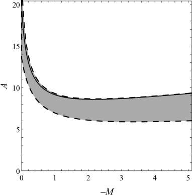
(a) $B=-10$

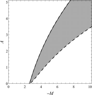
(b) $B=10$

Fig. 1: Two-dimensional sections of the parameter space $(M,A,B)$ satisfying (47) are colored gray (the boundary is indicated by dashed curves). The solid curves correspond to the parameters that yield $\Omega_{\rm m0}=0.3$, which almost overlap with the upper dashed curves.

IV.3 The solution

Having obtained the viable parameter region, now we are in a position to analyze the exact solution to (37). It is straightforward to integrate (37) to obtain the following algebraic equation for $\hat{H}$:

$$\hat{H}^{2}\left[2(1+3B\hat{H}+12M\hat{H}^{2})^{2}-3A^{2}(1-12M\hat{H}^{2})\right]+C(1+z)^{3}(1+3B\hat{H}+12M\hat{H}^{2})^{2}=0,$$ (48)

where the integration constant $C$ is determined from $\hat{H}(z=0)=1$ as

$$C=-2+\frac{3A^{2}(1-12M)}{(1+3B+12M)^{2}}.$$ (49)

Note that (40) is recovered in the limit $z\to-1$.

The Newton’s constant (28) and the effective gravitational coupling (25) are given, respectively, by

$$8\pi G_{N}M_{*}^{2} =1-\frac{18MA^{2}\hat{H}^{2}}{(1+3B\hat{H}+12M\hat{H}^{2})^{2}+18MA^{2}\hat{H}^{2}},$$ (50)

$$8\pi G_{\rm eff}M_{*}^{2} =8\pi G_{N}M_{*}^{2}+\frac{864M^{2}A^{2}(1-12M\hat{H}^{2})(1+3B\hat{H}+12M\hat{H}^{2})\hat{H}^{3}}{(1-36M\hat{H}^{2})\left[(1+3B\hat{H}+12M\hat{H}^{2})^{2}+18MA^{2}\hat{H}^{2}\right]^{2}}(1+z)\hat{H}^{\prime},$$ (51)

One can draw some information on the asymptotic behavior of these quantities from (51) and (50). In the infinite future, we have $\hat{H}^{\prime}\to 0$, and thus $G_{\rm eff}/G_{N}\to 1$, while for large $z$ where $\hat{H}\propto(1+z)^{3/2}$, we have

$$8\pi G_{\rm eff}M_{*}^{2}\to 1+\frac{A^{2}}{8M\hat{H}^{2}},\quad 8\pi G_{N}M_{*}^{2}\to 1-\frac{A^{2}}{8M\hat{H}^{2}}.$$ (52)

As an illustrative example, we plot the evolution of $\hat{H}$, $\epsilon_{H}$, and the gravitational couplings for $(M,A,B)=(-0.03,17,-10)$ in Fig. 2. Note that this parameter choice fulfills the viability conditions (47) (see Fig. 1). From these examples, we see that the background evolution is similar to the conventional $\Lambda$CDM model, while the evolution of the density fluctuations can be used to test the extended cuscuton as dark energy. The time variation of Newton’s constant can also be used to constrain the model, which, in the present case, is given by

$$\left.\frac{\dot{G}_{N}}{HG_{N}}\right|_{z=0}=\frac{54MA^{2}(1-12M)\left[2(1+3B+12M)^{2}-3A^{2}(1-12M)\right]}{\left[(1+3B+12M)^{2}+18MA^{2}\right]\left[2(1+3B+12M)^{3}-3A^{2}(1-36M-36MB)\right]},$$ (53)

while the observational bound reads $|\dot{G}_{N}/G_{N}|<0.02H_{0}$ Williams et al. (2004). One can check that the parameter choice $(M,A,B)=(-0.03,17,-10)$ satisfies this bound.

Fig. 2: Time evolution of $\hat{H}$, $\epsilon_{H}$, $G_{\rm eff}/G_{N}$, and $G_{N}/G_{N0}$, with $G_{N0}\coloneqq G_{N}(z=0)$. The solid lines correspond to $(M,A,B)=(-0.03,17,-10)$ and the dashed lines represent the result of the $\Lambda$CDM model with $\Omega_{\rm m0}=0.3$.

Before proceeding to the concluding section, let us mention some limiting cases where one of the model parameters in (29) is vanishing. When $\alpha=0$ (i.e., $A=0$), we obtain $\phi=0$ from (33), which contradicts the assumption that $\partial_{\mu}\phi$ is timelike (see §II). On the other hand, when $\mu=0$ (i.e., $M=0$), we obtain $G_{N}=G_{\rm eff}=(8\pi M_{*}^{2})^{-1}$ from (50) and (51), while the spacetime and the cuscuton field can evolve in a nontrivial manner.

V Conclusions

The extended cuscuton model is a general class of DHOST theories having a nondynamical scalar field when $\partial_{\mu}\phi$ is timelike. In §III, we studied homogeneous and isotropic cosmology in the extended cuscutons described by the action (1) in the presence of a matter field. We derived the background field equations and proposed the requirements [A]–[D] for these theories to serve as a viable dark energy model. Also, we investigated scalar perturbations to derive the evolution equation for the density fluctuations and the gravitational Poisson equations. In §IV, we turned to more specific discussions using a simple model (29) that can be solved analytically. The model parameter $\alpha$ appears as a coefficient of $\sqrt{2X}$, which is typical in the original cuscuton model. On the other hand, the parameters $\mu$ and $\beta$ characterize the difference from the original model. In order to avoid technical complexity, we defined dimensionless parameters $M$, $A$, and $B$, corresponding to $\mu$, $\alpha$, and $\beta$, respectively. We obtained the viable region in the parameter space $(M,A,B)$ which satisfies the requirements [A]–[D]. We also plotted the evolution of the dimensionless Hubble parameter $\hat{H}$, the Hubble slow-roll parameter $\epsilon_{H}$, the ratio of the effective gravitational coupling $G_{\mathrm{eff}}$ to the Newton’s constant $G_{N}$, and $G_{N}$ normalized by its present value for the parameter choice $(M,A,B)=(-0.03,17,-10)$, which lies in the viable parameter region. We found that the background evolution in this model can mimic the conventional $\Lambda$CDM model while the evolution of the density fluctuation deviates from the one in the $\Lambda$CDM case. Moreover, this set of parameters satisfies the observational constraint on the time variation of the Newton’s constant, $|\dot{G}_{N}/G_{N}|<0.02H_{0}$. Hence, one can test the extended cuscuton as dark energy by observations associated with the density fluctuations, e.g., the integrated Sachs-Wolfe effect or weak gravitational lensing, which we leave for future study.

As mentioned in §II, in general, extended cuscutons have an extra half DOF on top of two tensor modes Gao and Yao (2020). Nevertheless, at least up to linear perturbations on a homogeneous and isotropic background, we found no pathology caused by this half DOF. However, we may encounter some inconsistencies in higher-order perturbations or on another background. We hope to discuss this point in the near future.