Distributed Optimization With Event-triggered Communication via Input Feedforward Passivity

Abstract

In this work, we address the distributed optimization problem with event-triggered communication by the notion of input feedforward passivity (IFP). First, we analyze the distributed continuous-time algorithm over uniformly jointly strongly connected balanced digraphs in an IFP-based framework. Then, we propose a distributed event-triggered communication mechanism for this algorithm. Next, we discretize the continuous-time algorithm by the forward Euler method with a constant stepsize irrelevant to network size, and show that the discretization can be seen as a stepsize-dependent passivity degradation of the input feedforward passivity. Thus, the discretized system preserves the IFP property and enables the same event-triggered communication mechanism but without Zeno behavior due to the discrete-time nature. Finally, a numerical example is presented to illustrate our results.

I Introduction

Distributed optimization problem aims to optimize the sum of objective functions of agents cooperatively, where each agent estimates the optimal solution based on local information and information obtained from its neighbors through a communication network. It has been widely studied in recent years, and numerous algorithms have been proposed, which can be categorized into two groups, i.e., discrete-time algorithms [1, 2, 3, 4] and continuous-time algorithms [5, 6, 7, 8].

An important issue in distributed optimization is the relaxation of communication graph conditions, since the communication network may be unidirectional or even time-varying in practice. The work [5] generalizes the well-known proportional-integral (PI) algorithm to weight-balanced and strongly connected digraphs. A fully distributed adaptive algorithm for the design of parameters is proposed in [7]. The work [6] proposes a modified PI algorithm over weight-balanced and strongly connected switching digraphs. Recently, [9] incorporates a continuous-time push-sum algorithm to address the problem of general directed graphs. Besides, [10] proposes fully distributed algorithms over weight-balanced and uniformly jointly strongly connected digraphs based on input feedforward passivity (IFP). There are also many related works in the discrete-time setting (e.g., [1, 2, 3, 4] and references therein), while most of them adopt diminishing stepsizes or require global information.

Another critical problem for distributed optimization is event-triggered based communication motivated by practical issues in the communication network such as network congestion, limited bandwidth, and energy consumption. A centralized event-triggered strategy is proposed in [6]. An encoder-decoder event-trigger communication mechanism is introduced in [11]. An edge-based event-triggered method is proposed in [12]. The work [13] considers event-triggered communication for distributed optimization with geometric constraints. However, the abovementioned works only consider cases with undirected or fixed communication networks and cannot apply to directed and switching networks. Recently, a periodic sampling communication mechanism is proposed in [14] over weight-balanced and uniformly jointly strongly connected digraphs for resource allocation problems. Considering distributed algorithms under event-triggered control over uniformly jointly strongly connected digraphs is of great significance, since the communication effort can be greatly reduced due to the lack of graph connectivity or consecutive communication. To the best of our knowledge, this problem has not been addressed yet.

In this work, we consider a distributed optimization problem over uniformly jointly strongly connected balanced graphs and propose a distributed event-triggered communication scheme for both the continuous-time and discrete-time algorithms via IFP. The continuous-time algorithm has been proposed in [10, 6], while its discrete-time counterpart is first introduced here.

II Preliminaries

II-A Notation

Let $\mathbb{R}$ be the set of real numbers. The Kronecker product is denoted as $\otimes$. Let $\left\|\cdot\right\|$ denote the 2-norm of a vector and also the induced 2-norm of a matrix. Given a symmetric matrix $M\in\mathbb{R}^{m\times m}$, $M>0$ $(M\geq 0)$ means that $M$ is positive definite (positive semi-definite). Let $I$ and $\mathbf{0}$ denote the identity matrix and zero matrix with proper dimensions, respectively. $\mathbf{1}_{m}:=(1,\ldots,1)^{T}\in\mathbb{R}^{m}$ denotes the vector with all ones.

II-B Convex Analysis

A differentiable function $f:\mathbb{R}^{m}\rightarrow\mathbb{R}$ is convex over a convex set $\mathcal{X}\subset\mathbb{R}^{m}$ if and only if $\left(\nabla f(x)-\nabla f(y)\right)^{T}(x-y)\geq 0$, $\forall x,~{}y\in\mathcal{X}$. It is $\mu$-strongly convex if and only if $\left(\nabla f(x)-\nabla f(y)\right)^{T}(x-y)\geq\mu\left\|x-y\right\|^{2}$, or equivalently, $f(y)\geq f(x)+\nabla f(x)^{T}(y-x)+\frac{\mu}{2}\left\|y-x\right\|^{2}$, $\forall x,y\in\mathcal{X}$. An operator $\mathbf{f}:\mathbb{R}^{m}\rightarrow\mathbb{R}^{m}$ is $l$-Lipschitz continuous over a set $\mathcal{X}\in\mathbb{R}^{m}$ if $\left\|\mathbf{f}(x)-\mathbf{f}(y)\right\|\leq l\left\|x-y\right\|$, $\forall x,y\in\mathcal{X}$.

II-C Communication Network and Graph Theory

The communication network is represented by a graph $\mathcal{G}=(\mathcal{N},\mathcal{E})$, where $\mathcal{N}=\{1,\ldots,N\}$ is the node or agent set, $\mathcal{E}\subset\mathcal{N}\times\mathcal{N}$ is the edge set. The edge $(i,j)\in\mathcal{E}$ means that agent $i$ can send information to agent $j$. The graph $\mathcal{G}$ is said to be undirected if $(i,j)\in\mathcal{E}\Leftrightarrow(j,i)\in\mathcal{E}$ and directed otherwise. The adjacency matrix $A=[a_{ij}]$ of $\mathcal{G}$ is defined as $a_{ii}=0$; $a_{ij}>0$ if $(j,i)\in\mathcal{E}$, and $a_{ij}=0$, otherwise. $\mathcal{G}$ is said to be strongly connected if there exists a sequence of successive edges between any two agents. The in-degree and out-degree of the $i$th agent are $d_{in}^{i}=\sum_{j=1}^{N}a_{ij}$ and $d_{out}^{i}=\sum_{j=1}^{N}a_{ji}$, respectively. The graph $\mathcal{G}$ is said to be weight-balanced if $d_{in}^{i}=d_{out}^{i},~{}\forall i\in\mathcal{N}$. The Laplacian matrix of $\mathcal{G}$ is defined as $L=\textrm{diag}\{A\mathbf{1}_{N}\}-A$. Clearly, $L\mathbf{1}_{N}=\mathbf{0}$. Moreover, if $\mathcal{G}$ is weight-balanced, then $\mathbf{1}_{N}^{T}L=\mathbf{0}$. A time-varying graph $\mathcal{G}(t)$ with fixed nodes is said to be uniformly jointly strongly connected (UJSC) if there exists a $T>0$ such that for any $t_{k}$, the union $\cup_{t\in[t_{k},t_{k}+T]}\mathcal{G}(t)$ is strongly connected.

II-D Passivity

Consider a nonlinear system $\Sigma$ described by

$$\begin{cases}x^{+}=F\left(x,u\right)\\ y=H\left(x,u\right)\end{cases}$$ (1)

where $x\in\mathcal{X}\subset\mathbb{R}^{n}$, $u\in\mathcal{U}\subset\mathbb{R}^{m}$ and $y\in\mathcal{Y}\subset\mathbb{R}^{m}$ are the state, input and output, respectively, and $\mathcal{X}$, $\mathcal{U}$ and $\mathcal{Y}$ are the state, input and output spaces, respectively. $x^{+}$ denotes the derivative of the state in the continuous-time (CT) case and the state at the next time step in the discrete-time (DT) case. The nonlinear functions $F:\mathcal{X}\times\mathcal{U}\rightarrow\mathbb{R}^{n}$, $H:\mathcal{X}\times\mathcal{U}\rightarrow\mathcal{Y}$ are assumed to be sufficiently smooth.

System $\Sigma$ is said to be passive if there exists a continuously differentiable positive semi-definite function $V(x)$, called the storage function, such that $\dot{V}(x)\leq u^{T}y,~{}\forall x\in\mathcal{X},~{}u\in\mathcal{U}$ in CT case (or, $V\left(x(k+1)\right)-V\left(x(k)\right)\leq u^{T}y,~{}\forall x\in\mathcal{X},~{}u\in\mathcal{U},$ in DT case). Moreover, it is said to be input feedforward passive (IFP) if $\dot{V}(x)\leq u^{T}y-\nu u^{T}u$ for CT case (or, $V\left(x(k+1)\right)-V\left(x(k)\right)\leq u^{T}y-\nu u^{T}u$ for DT case), for some $\nu\in\mathbb{R}$, denoted as IFP($\nu$). The sign of the IFP index $\nu$ denotes an excess or shortage of passivity.

II-E Problem Formulation

Consider a distributed optimization problem among a group of agents

$$\min_{\mathrm{x}}\sum_{i=1}^{N}f_{i}(\mathrm{x})$$ (2)

where $f_{i}:\mathbb{R}^{m}\rightarrow\mathbb{R}$ is the local objective function for agent $i$, $\forall i\in\mathcal{N}=\{1,\ldots,N\}$ and $\mathrm{x}\in\mathbb{R}^{m}$ is the decision variable. We consider problem (2) with the following assumptions.

Assumption 1.

Each local function $f_{i}$ is sufficiently smooth, $\mu_{i}$-strongly convex and has $l_{i}$-Lipschitz continuous gradient.

Assumption 2.

The time-varying communication digraph $\mathcal{G}$ is weight-balanced pointwise in time and UJSC.

Assumption 3.

The communication protocol is designed such that both the sender and receiver of an edge are aware of its existence.

Remark 1.

3 is a standard assumption in the literature, where each agent knows its out-degree [1, 4]. Then, each agent can locally manipulate its in/out-degree to render the global graph weight-balanced, while the strong connectedness is not required pointwise in time. Moreover, no restriction on the switching rules is imposed. The graph can change continuously provided 2 and 3 are satisfied.

III Continuous-time Algorithm

III-A IFP-based Distributed Algorithm

We adopt a distributed algorithm that consists of a group of input feedforward passive system in the following form to solve problem (2),

$$\dot{x}_{i}= -\alpha\nabla f_{i}(x_{i})-\lambda_{i}$$ (3a)

$$\dot{\lambda}_{i}= -u_{i}$$ (3b)

where $x_{i}\in\mathbb{R}^{m}$ is the decision variable for agent $i$, $\lambda_{i}\in\mathbb{R}^{m}$ is an auxiliary state for agent $i$ to track the difference between neighboring agents. In the above individual system, $u_{i}$ is the system input taking the diffusive couplings of $x_{i}$, i.e.,

$$u_{i}= \beta\sum_{j=1}^{N}a_{ij}(t)(x_{j}-x_{i}).$$ (4)

In the above equations, $\alpha>0$, $\beta>0$ are parameters to be designed. To ensure optimality under input (4), $\lambda_{i}$ should satisfy $\sum_{i=1}^{N}\lambda_{i}(0)=\mathbf{0}$, which can be fulfilled by setting $\lambda_{i}(0)=0$, for all $i\in\mathcal{N}$.

Note that algorithm (3) is a simplified version of the algorithm reported in [6, 10] in which (3a) becomes $\dot{x}_{i}=-\alpha\nabla f_{i}(x_{i})-\lambda_{i}+u_{i}$. In this work, we first analyze the algorithm (3) with (4) in an input-feedforward passivity-based framework, and then propose an event-triggered mechanism for the algorithmic dynamics.

Define $\left(x_{i}^{*},\lambda_{i}^{*}\right)$ as the equilibrium point of system (3). Then, equilibrium point in (3b) ensures that $u_{i}\equiv 0$, which further gives $x_{i}^{*}=x_{j}^{*}$, $\forall i,j\in\mathcal{N}$. Summing up (3a), $\forall i\in\mathcal{N}$, one has

$$\begin{array}[]{rl}-\alpha\displaystyle\sum_{i=1}^{N}\nabla f_{i}(x_{i}^{*})=\sum_{i=1}^{N}\lambda_{i}^{*}=(\mathbf{1}_{N}^{T}\otimes I)\lambda^{*}=\sum_{i=1}^{N}\lambda_{i}(0)=\mathbf{0}\end{array}$$

with $\lambda^{*}=({\lambda_{1}^{*}}^{T},\ldots,{\lambda_{N}^{*}}^{T})^{T}$. The third equality in the above equation follows from $\mathbf{1}_{N}^{T}L=\mathbf{0}$. Then $x_{i}^{*}$ is the unique optimal solution to problem (2) (see [10] for details). Denote $\Delta x_{i}=x_{i}-x_{i}^{*}$, $\Delta\lambda_{i}=\lambda_{i}-\lambda_{i}^{*}$, and

$$\nabla f_{i}(x_{i})-\nabla f_{i}(x_{i}^{*})=B_{x_{i}}\Delta x_{i}$$ (6)

where $B_{x_{i}}$ is defined as $B_{x_{i}}=\int_{0}^{1}\nabla^{2}f_{i}(x_{i}^{*}+\tau(x_{i}-x_{i}^{*}))d\tau$. It follows that $\Delta\dot{x}_{i}=-\alpha B_{x_{i}}\Delta x_{i}-\Delta\lambda_{i}.$ Under Assumption 1, we have $\mu_{i}I\leq B_{x_{i}}\leq l_{i}I$.

Lemma 1.

Under Assumption 1, system (3) is IFP($\nu_{i}$) from $u_{i}$ to $\Delta x_{i}$ with index $\nu_{i}=-\frac{1}{\alpha^{2}\mu_{i}^{2}}$ with respect to the storage function

$$\begin{array}[]{rl}V_{i}=&\frac{1}{\alpha\mu_{i}}\left\|\Delta\dot{x}_{i}\right\|^{2}-\Delta x_{i}^{T}\Delta\lambda_{i}+\alpha\nabla f_{i}(x_{i}^{*})^{T}\Delta x_{i}\\ &+\alpha\left(f_{i}(x_{i}^{*})-f_{i}(x_{i})\right).\end{array}$$

Proof.

The strong convexity of $f_{i}(x_{i})$ provides that

$$\begin{array}[]{rl}&\alpha\left(f_{i}(x_{i}^{*})-f_{i}(x_{i})\right)+\alpha\nabla f_{i}(x_{i}^{*})^{T}\Delta x_{i}\\ \geq&\Delta x_{i}^{T}\left(-\alpha B_{x_{i}}+\frac{\alpha\mu_{i}}{2}I\right)\Delta x_{i}.\end{array}$$

Therefore, it can be derived that

$$V_{i}\geq\left(\begin{smallmatrix}\alpha B_{x_{i}}\Delta x_{i}\\ \Delta\lambda_{i}\end{smallmatrix}\right)^{T}{R}_{i}\left(\begin{smallmatrix}\alpha B_{x_{i}}\Delta x_{i}\\ \Delta\lambda_{i}\end{smallmatrix}\right)$$

where ${R}_{i}=\left(\begin{smallmatrix}\frac{I}{\alpha\mu_{i}}-\frac{1}{\alpha}B_{x_{i}}^{-1}+\frac{\mu_{i}}{2\alpha}B_{x_{i}}^{-2}&\frac{I}{\alpha\mu_{i}}-\frac{1}{2\alpha}B_{x_{i}}^{-1}\\ \frac{I}{\alpha\mu_{i}}-\frac{1}{2\alpha}B_{x_{i}}^{-1}&\frac{I}{\alpha\mu_{i}}\end{smallmatrix}\right)>0$. Thus, $V_{i}$ is positive definite and radially unbounded with respect to $\left\|\left(\begin{smallmatrix}\alpha B_{x_{i}}\Delta x_{i}\\ \Delta\lambda_{i}\end{smallmatrix}\right)\right\|$. Taking the derivative of $V_{i}$ along system (3) gives

$$\begin{array}[]{rl}\dot{V_{i}}=&\frac{1}{\alpha\mu_{i}}\frac{d\left\|\Delta\dot{x}_{i}\right\|^{2}}{dt}+\frac{d(-\Delta x_{i}^{T}\Delta\lambda_{i})}{dt}+\\ &\alpha\cdot\frac{d\left(f_{i}(x_{i}^{*})-f_{i}(x_{i})+\nabla f_{i}(x_{i}^{*})^{T}\Delta x_{i}\right)}{dt}\\ \leq&-2\left\|\Delta\dot{x}_{i}\right\|^{2}+\frac{2}{\alpha\mu_{i}}\Delta\dot{x}_{i}^{T}u_{i}+\Delta x_{i}^{T}u_{i}\\ &-\left(\alpha B_{x_{i}}\Delta x_{i}+\Delta\lambda_{i}\right)^{T}\Delta\dot{x}_{i}\\ =&-||\Delta\dot{x}_{i}||^{2}+\frac{2}{\alpha\mu_{i}}\Delta\dot{x}_{i}^{T}u_{i}+\Delta x_{i}^{T}u_{i}\\ \leq&\Delta x_{i}^{T}u_{i}+\frac{1}{\alpha^{2}\mu_{i}^{2}}||u_{i}||^{2},\end{array}$$

which completes the proof. ∎

Lemma 2 ([10]).

Under Assumption 1 and 2, the states of algorithm (3) with initial condition $\sum_{i=1}^{N}\lambda_{i}(0)=\mathbf{0}$ will converge to the optimal solution to problem (2) if the following condition holds,

$$|\nu_{i}|\beta d_{in}^{i}(t)<\frac{1}{2},~{}\forall i\in\mathcal{N},~{}\forall t\geq 0$$ (9)

where $d_{in}^{i}(t)$ denotes the in-degree of the $i$th agent and $\nu_{i}$ is the IFP index defined in Lemma 1.

This lemma characterizes the design of parameters $\alpha$, $\beta$ through input-feedforward passivity. In practice, we can fix one variable and design the other one. Lemma 2 can be proved by considering the Lyapunov function candidate $V=\sum_{i=1}^{N}V_{i}$. Readers can refer to [10] for the proof.

III-B Event-triggered Mechanism

In this subsection, we reconsider the algorithm in (3) by incorporating an event-triggered communication mechanism, i.e., instead of transmitting the real-time $x_{i}$, an event-triggered-based input is considered,

$$u_{i}= \beta\sum_{i=1}^{N}a_{ij}(t)(\hat{x}_{j}-\hat{x}_{i})$$ (10)

where $\hat{x}_{i},\ i\in\mathcal{N}$ denotes the latest sampled state of agent $i$ that has been transmitted to its neighbors and $\hat{x}_{i}(0):=x_{i}(0)$. In (10), each agent only updates its current state $x_{i}$ to its out-neighbors when the local error signal $e_{i}(t)=x_{i}(t)-\hat{x}_{i}(t)$ exceeds a threshold depending on the latest received state of $x_{j}$ from its in-neighbors. In this work, the triggering condition is

$$\left\|e_{i}(t)\right\|^{2}\geq\frac{c_{i}}{d^{i}_{in}(t)}\left(\frac{1}{2}-|\nu_{i}|\beta d_{in}^{i}(t)\right)^{2}\sum_{j=1}^{N}a_{ij}(t)\left\|\hat{x}_{j}-\hat{x}_{i}\right\|^{2}$$ (11)

where $c_{i}\in(0,1)$ is a constant. This triggering condition is fully distributed since only local information is needed.

In a time-varying graph, we stipulate that, whenever a link between two agents appears, the sender sends its last triggered state to the receiver, which is not considered as a “triggering”. Whenever a link disappears, the receiver modifies (10) accordingly such that the disconnection between agents is not confused with the “connected but non-triggering” case. This can be guaranteed by 3.

The following theorem presents the convergence to the global optimal solution under event-triggered communication.

Theorem 1.

Under Assumptions 1–3, if $\alpha,\beta$ are designed such that (9) holds, and the triggering instant for agent $i$, $i\in\mathcal{N}$ to transmit its current information of $x_{i}$ is chosen whenever $d^{i}_{in}(t)>0$ and the triggering condition (11) is satisfied. Suppose there exists a solution to system (3) under event-triggered control (10), (11) for all $t\geq 0$. Then the states with initial condition $\sum_{i=1}^{N}\lambda_{i}(0)=\mathbf{0}$ will converge to the optimal solution to problem (2).

Proof.

Consider the Lyapunov function candidate $V=\sum_{i=1}^{N}V_{i}\geq 0$, where $V_{i}$ was defined in (1). From Lemma 1, its derivative along (3) and (10) yields

$$\dot{V}\leq {\displaystyle\sum_{i=1}^{N}}\Delta x_{i}^{T}u_{i}-\nu_{i}u_{i}^{T}u_{i}$$

$$= {\displaystyle\sum_{i=1}^{N}}\left(\beta\Delta x_{i}^{T}\displaystyle\sum_{j=1}^{N}a_{ij}(t)\left(\Delta\hat{x}_{j}-\Delta\hat{x}_{i}\right)\right)$$

$$+{\displaystyle\sum_{i=1}^{N}}\beta^{2}|\nu_{i}|\bigg{\|}\displaystyle\sum_{j=1}^{N}a_{ij}(t)\left(\Delta\hat{x}_{j}-\Delta\hat{x}_{i}\right)\bigg{\|}^{2}$$

$$= {\displaystyle\sum_{i=1}^{N}}\left(\beta\left(\Delta\hat{x}_{i}+e_{i}\right)^{T}{\displaystyle\sum_{j=1}^{N}}a_{ij}(t)\left(\Delta\hat{x}_{j}-\Delta\hat{x}_{i}\right)\right)$$

$$+{\displaystyle\sum_{i=1}^{N}}\beta^{2}|\nu_{i}|\bigg{\|}{\displaystyle\sum_{j=1}^{N}}a_{ij}(t)\left(\hat{x}_{j}-\hat{x}_{i}\right)\bigg{\|}^{2}$$

$$= \beta{\displaystyle\sum_{i=1}^{N}}\left({\displaystyle\sum_{j=1}^{N}}e_{i}^{T}a_{ij}(t)\left(\hat{x}_{j}-\hat{x}_{i}\right)+{\displaystyle\sum_{j=1}^{N}}a_{ij}(t)\Delta\hat{x}_{i}^{T}\Delta\hat{x}_{j}\right.$$

$$\left.-{\displaystyle\sum_{j=1}^{N}}a_{ij}(t)\Delta\hat{x}_{i}^{T}\Delta\hat{x}_{i}+\beta|\nu_{i}|\bigg{\|}{\displaystyle\sum_{j=1}^{N}}a_{ij}(t)\left(\hat{x}_{j}-\hat{x}_{i}\right)\bigg{\|}^{2}\right)$$

where $\Delta\hat{x}_{i}:=\hat{x}_{i}-x_{i}^{*}$. The second equality in the above equation holds since $e_{i}=x_{i}-\hat{x}_{i}=\Delta x_{i}-\Delta\hat{x}_{i}$. Observe that

$$\begin{array}[]{rl}e_{i}^{T}a_{ij}(t)\left(\hat{x}_{j}-\hat{x}_{i}\right)\leq a_{ij}(t)\left(\frac{1}{2\theta}\left\|e_{i}\right\|^{2}+\frac{\theta}{2}\left\|\hat{x}_{j}-\hat{x}_{i}\right\|^{2}\right)\end{array}$$

with $\theta>0$, and

$$\begin{array}[]{rl}&{\displaystyle\sum_{i=1}^{N}\sum_{j=1}^{N}}a_{ij}(t)\Delta\hat{x}_{i}^{T}\Delta\hat{x}_{j}-{\displaystyle\sum_{i=1}^{N}\sum_{j=1}^{N}}a_{ij}(t)\Delta\hat{x}_{i}^{T}\Delta\hat{x}_{i}\\ =&-\frac{1}{2}{\displaystyle\sum_{i=1}^{N}\sum_{j=1}^{N}}a_{ij}(t)\left(\Delta\hat{x}_{i}^{T}\Delta\hat{x}_{i}-2\Delta\hat{x}_{i}^{T}\Delta\hat{x}_{j}+\Delta\hat{x}_{j}^{T}\Delta\hat{x}_{j}\right)\\ =&-\frac{1}{2}{\displaystyle\sum_{i=1}^{N}\sum_{j=1}^{N}}a_{ij}(t)\left\|\hat{x}_{j}-\hat{x}_{i}\right\|^{2}\end{array}$$

where the first equality holds because the graph $\mathcal{G}(t)$ is balanced. Moreover, by Cauchy–Schwarz inequality, one has

$$\bigg{\|}\sum_{j=1}^{N}a_{ij}(t)\left(\hat{x}_{j}-\hat{x}_{i}\right)\bigg{\|}^{2}\leq d_{in}^{i}(t)\sum_{j=1}^{N}a_{ij}(t)\left\|\hat{x}_{j}-\hat{x}_{i}\right\|^{2}.$$

Hence, it can be further obtained that

$$\begin{array}[]{rl}\dot{V}\leq&-\frac{\beta}{2}\displaystyle\sum_{i=1}^{N}\sum_{j=1}^{N}a_{ij}(t)\left(-\frac{\left\|e_{i}\right\|^{2}}{\theta}+(1-2|\nu_{i}|\beta d_{in}^{i}(t)-\theta)\right.\\ &\left.\cdot\left\|\hat{x}_{j}-\hat{x}_{i}\right\|^{2}\vphantom{\displaystyle\sum_{j=1}^{N}}\right).\end{array}$$

A sufficient condition to ensure $\dot{V}\leq 0$ is

$$\left\|e_{i}\right\|^{2}\leq\frac{\theta}{d^{i}_{in}(t)}\left(1-2|\nu_{i}|\beta d_{in}^{i}(t)-\theta\right)\sum_{j=1}^{N}a_{ij}(t)\left\|\hat{x}_{j}-\hat{x}_{i}\right\|^{2}.$$

The right hand side of the above inequality obtains the maximum value when $\theta=\frac{1}{2}-|\nu_{i}|\beta d_{in}^{i}(t)$. Define $c_{i}\in(0,1)$, then the triggering condition (11) guarantees $\dot{V}\leq 0$. Define the domain $\Omega_{0}=\{(x,\lambda)|V(x,\lambda)\leq V(x(0),\lambda(0))\}$ with $x=(x_{1}^{T},\ldots,x_{N}^{T})^{T}$, $\lambda=(\lambda_{1}^{T},\ldots,\lambda_{N}^{T})^{T}$. Because $\dot{V}\leq 0$, it is clear that all system trajectories are bounded and contained within the domain $\Omega_{0}$. Next, define the domain $\Omega_{e}=\{(x,\lambda)|\dot{V}=0\}$. It is clear that $\|\dot{x}_{i}\|$ and $\|\dot{\lambda}_{i}\|$ are bounded for any bounded $x_{i}$, $\lambda_{i}$, $\forall i\in\mathcal{N}$. Invoking the Invariance Principle [15, Theorem 2.3], all limit points of the bounded trajectory belong to the domain $\Omega_{f}=\Omega_{0}\cap\Omega_{e}$, which implies $\lim_{t\rightarrow\infty}\|e_{i}(t)\|=0$ and $\lim_{t\rightarrow\infty}\hat{x}_{i}=\lim_{t\rightarrow\infty}\hat{x}_{j}$. It follows that $\lim_{t\rightarrow\infty}x_{i}=\lim_{t\rightarrow\infty}x_{j}$. Summing up (3a) similarly to (III-A) we obtain $\lim_{t\rightarrow\infty}(x_{i},\lambda_{i})=(x_{i}^{*},\lambda_{i}^{*})$, which completes the proof.

∎

Remark 2.

To avoid the Zeno behavior in practice, one can implement the following triggering condition instead,

$$\begin{array}[]{rl}\left\|e_{i}(t)\right\|^{2}\geq\max\left\{\frac{c_{i}\left(\frac{1}{2}-\beta|\nu_{i}|\right)^{2}}{d^{i}_{in}(t)}\displaystyle\sum_{j=1}^{N}a_{ij}(t)\left\|\hat{x}_{j}-\hat{x}_{i}\right\|^{2},\zeta\right\}\end{array}$$

where $\zeta>0$ is an small predefined error. However, under this condition no exact consensus but only practical consensus of $x_{i}$, $i\in\mathcal{N}$ can be reached since this condition only guarantees Lyapunov boundedness, and the closer $\zeta$ gets to zero, the more accurate the result can be. Nevertheless, we will see in the next section that the event-triggered scheme (11) can be readily applied to the discretized algorithm, wherein Zeno behavior is avoided naturally.

IV Discrete-time Algorithm

In this section, we study the discretization of the continuous-time algorithm (3). By applying the forward Euler method to algorithm (3) with respect to a constant stepsize $\delta>0$, we can obtain the following discrete-time algorithm

$${x}_{i}(k+1)= {x}_{i}(k)-\delta\left(\alpha\nabla f_{i}({x}_{i}(k))+{\lambda}_{i}(k)\right)$$ (12a)

$${\lambda}_{i}(k+1)= {\lambda}_{i}(k)-\delta u_{i}(k)$$ (12b)

where ${u}_{i}(k)$ is the input taking the diffusive couplings of $x_{i}(k)$, i.e.,

$$u_{i}(k)=\beta\displaystyle\sum_{j=1}^{N}a_{ij}(k)\left({x}_{j}(k)-{x}_{i}(k)\right).$$

IV-A IFP Preservation

We analyze the discrete-time algorithm from the perspective of passivity in this subsection.

Lemma 3 (IFP preservation).

By selecting an appropriate stepsize

$$\delta<\frac{1}{\alpha}\frac{4l_{i}-2\mu_{i}}{2l_{i}^{2}-\mu_{i}^{2}},\quad\forall i\in\mathcal{N},$$ (14)

system (12) is IFP($\tilde{\nu}_{i}$) from ${u}_{i}$ to $\Delta{x}_{i}$ with

$$\tilde{\nu}_{i}=-\frac{\left(\frac{1}{\alpha\mu_{i}}+\delta\left(\frac{1}{2}+\frac{l_{i}}{\mu_{i}}\right)\right)^{2}}{\alpha\delta\left(\frac{\mu_{i}}{2}-\frac{l_{i}^{2}}{\mu_{i}}\right)+\frac{2l_{i}}{\mu_{i}}-1}.$$ (15)

Proof.

Denote ${z}_{i}(k)=\alpha\nabla{f}_{i}({x}_{i}(k))+{\lambda}_{i}(k)$. Adopt the storage function $\tilde{V}_{i}=\frac{1}{\delta}V_{i}$, where $V_{i}=$ First, we have

$${V}_{i}(k+1)-{V}_{i}(k)$$

$$= \frac{1}{\alpha\mu_{i}}\left(\|z_{i}(k+1)\|^{2}-\|z_{i}(k)\|^{2}\right)$$ (16a)

$$-\Delta x_{i}(k+1)^{T}\Delta\lambda_{i}(k+1)+\Delta x_{i}(k)^{T}\Delta\lambda_{i}(k)$$ (16b)

$$+\alpha\left(f_{i}(x_{i}(k))-f_{i}(x_{i}(k+1))+\nabla f_{i}(x^{*}_{i})^{T}\cdot\right.$$

$$\left.(x_{i}(k+1)-x_{i}(k))\right)$$ (16c)

Denote $\nabla f_{i}(x_{i}(k+1))-\nabla f_{i}(x_{i}(k))=B_{x_{i}^{+}}(x_{i}(k+1)-x_{i}(k))$, where $B_{x_{i}^{+}}$ is definied similarly as $B_{x_{i}}$ in (6), and is a positive definite matrix satisfying $\mu_{i}I\leq B_{x_{i}^{+}}\leq l_{i}I$. Then, (16a) becomes

$$\begin{array}[]{rl}&\frac{1}{\alpha\mu_{i}}\left(\|\alpha\nabla f_{i}(x_{i}(k+1))+\lambda_{i}(k+1)\|^{2}-\|z_{i}(k)\|^{2}\right)\\ =&\frac{1}{\alpha\mu_{i}}\left(\|\alpha(\nabla f_{i}(x_{i}(k))-B_{x_{i}^{+}}\delta z_{i}(k))+\lambda_{i}(k)-\delta u_{i}(k)\|^{2}\right.\\ &\left.-\|z_{i}(k)\|^{2}\vphantom{B_{x_{i}^{+}}}\right)\\ =&\frac{1}{\alpha\mu_{i}}\left(\left\|\left(I-\alpha\delta B_{x_{i}^{+}}\right)z_{i}(k)-\delta u_{i}(k)\right\|^{2}-\|z_{i}(k)\|^{2}\right)\\ =&z_{i}(k)^{T}\left(\frac{\alpha\delta^{2}}{\mu_{i}}B_{x_{i}^{+}}^{2}-\frac{2\delta}{\mu_{i}}B_{x_{i}^{+}}\right)z_{i}(k)+\frac{\delta^{2}}{\alpha\mu_{i}}\|u_{i}(k)\|^{2}\\ &-z_{i}(k)^{T}\left(\frac{2\delta}{\alpha\mu_{i}}I-\frac{2\delta^{2}}{\mu_{i}}B_{x_{i}^{+}}\right)u_{i}(k)\end{array}$$

where the first and second qualities follow from the definition of $z_{i}(k)$. By substituting (12) into (16b), it can be readily obtained that (16b) equals to

$$\Delta x_{i}(k)^{T}\Delta\lambda_{i}(k)-\left(\Delta x_{i}(k)-\delta z_{i}(k)\right)^{T}\left(\Delta\lambda_{i}(k)-\delta u_{i}(k)\right)$$

$$= \delta z_{i}(k)^{T}\Delta\lambda_{i}(k)-\delta^{2}z_{i}(k)^{T}u_{i}(k)+\delta\Delta x_{i}(k)^{T}u_{i}(k).$$

Moreover, by the strong convexity of $f_{i}$, (16c) satisfies

$$\begin{array}[]{rl}&\alpha\left(f_{i}(x_{i}(k))-f_{i}(x_{i}(k+1))+\nabla f_{i}(x^{*}_{i})^{T}(-\delta z_{i}(k))\right)\\ \leq&\alpha\left(\vphantom{\frac{\mu_{i}}{2}}-\nabla f_{i}(x_{i}(k))^{T}\left(x_{i}(k+1)-x_{i}(k)\right)\right.\\ &\left.-\frac{\mu_{i}}{2}\|x_{i}(k+1)-x_{i}(k)\|^{2}-\delta\nabla f_{i}(x^{*}_{i})^{T}z_{i}(k)\right)\\ =&\alpha\delta\left(\nabla f_{i}(x_{i}(k))-\nabla f_{i}(x_{i}^{*})\right)^{T}z_{i}(k)-\frac{\alpha\mu_{i}}{2}\delta^{2}\|z_{i}(k)\|^{2}\end{array}$$

where the equality follows from (12a). Summing up (16a), (16b) and (16c) and by the definition of $\tilde{V}_{i}$, we obtain

$$\begin{array}[]{rl}&\tilde{V}_{i}(k+1)-\tilde{V}_{i}(k)\\ \leq&z_{i}(k)^{T}\left(\frac{\alpha\delta}{\mu_{i}}B_{x_{i}^{+}}^{2}-\frac{2}{\mu_{i}}B_{x_{i}^{+}}+\left(1-\frac{\alpha\delta\mu_{i}}{2}\right)I\right)z_{i}(k)\\ &-z_{i}(k)^{T}\left(\left(\frac{2}{\alpha\mu_{i}}+\delta\right)I-\frac{2\delta}{\mu_{i}}B_{x_{i}^{+}}\right)u_{i}+\Delta x_{i}(k)^{T}u_{i}(k)\\ &+\frac{\delta}{\alpha\mu_{i}}\|u_{i}(k)\|^{2}\\ =&\left(\begin{smallmatrix}z_{i}(k)\\ u_{i}(k)\end{smallmatrix}\right)^{T}M\left(\begin{smallmatrix}z_{i}(k)\\ u_{i}(k)\end{smallmatrix}\right)+\Delta x_{i}(k)^{T}u_{i}(k)-\tilde{\nu}_{i}\|u_{i}(k)\|^{2}\end{array}$$

where $M=\left(\begin{smallmatrix}\frac{\alpha\delta}{\mu_{i}}B_{x_{i}^{+}}^{2}-\frac{2}{\mu_{i}}B_{x_{i}^{+}}+\left(1-\frac{\alpha\delta\mu_{i}}{2}\right)I&\left(\frac{1}{\alpha\mu_{i}}+\frac{\delta}{2}\right)I-\frac{\delta}{\mu_{i}}B_{x_{i}^{+}}\\ *&\tilde{\nu}_{i}I\end{smallmatrix}\right)$, and the inequality follows from the definition of $z_{i}(k)$. Apparently, since $\mu_{i}I\leq B_{x_{i}^{+}}\leq l_{i}I$, one has

$$M\leq\left(\begin{smallmatrix}\frac{\alpha\delta l_{i}^{2}}{\mu_{i}}-\frac{2l_{i}}{\mu_{i}}+1-\frac{\alpha\delta\mu_{i}}{2}&\frac{1}{\alpha\mu_{i}}+\frac{\delta}{2}+\frac{\delta l_{i}}{\mu_{i}}\\ *&\tilde{\nu}_{i}\end{smallmatrix}\right)\otimes I.$$

Then, $M\leq 0$ if $\delta<\frac{1}{\alpha}\frac{4l_{i}-2\mu_{i}}{2l_{i}^{2}-\mu_{i}^{2}}$ and $\tilde{\nu}_{i}\leq-\frac{\left(\frac{1}{\alpha\mu_{i}}+\delta\left(\frac{1}{2}+\frac{l_{i}}{\mu_{i}}\right)\right)^{2}}{\alpha\delta\left(\frac{\mu_{i}}{2}-\frac{l_{i}^{2}}{\mu_{i}}\right)+\frac{2l_{i}}{\mu_{i}}-1}$. Thus, given an appropriate constant $\delta$, we obtain $\tilde{V}_{i}(k+1)-\tilde{V}_{i}(k)\leq\Delta x_{i}^{T}u_{i}-\tilde{\nu}_{i}\|u_{i}\|^{2}$, which completes the proof. ∎

Remark 3.

The stepsize $\delta$ obtained in condition (14) is constant and non-diminishing. It is independent of network size and thus less conservative compared to many works in the literature [1, 2, 3, 4]. Moreover, it can also be easily estimated distributedly given the bounds of indices $\mu_{i}$ and $l_{i}$, $\forall i\in\mathcal{N}$. It can be observed that (15) characterizes the passivity degradation over discretization. If the stepsize $\delta$ is infinitely small, then $\lim_{\delta\rightarrow 0^{+}}M=\left(\begin{smallmatrix}I-\frac{2}{\mu_{i}}B_{x_{i}^{+}}&{\alpha\mu_{i}}I\\ *&\tilde{\nu}_{i}I\end{smallmatrix}\right)\leq\left(\begin{smallmatrix}-I&{\alpha\mu_{i}}I\\ *&\tilde{\nu}_{i}I\end{smallmatrix}\right)$ and $\lim_{\delta\rightarrow 0^{+}}\tilde{\nu}=-\frac{1}{\alpha^{2}\mu_{i}^{2}}$, which recovers to the IFP index $\nu_{i}$ for the continuous-time system.

Next, we study the convergence of the algorithm following similar lines of Lemma 2.

Theorem 2.

Under Assumptions 1–3, the states of algorithm (12), (IV) with initial condition $\sum_{i=1}^{N}\lambda_{i}(0)=\mathbf{0}$ will converge to the optimal solution to problem (2) if the stepsize $\delta<\frac{1}{\alpha}\frac{4l_{i}-2\mu_{i}}{2l_{i}^{2}-\mu_{i}^{2}}$, $\forall i\in\mathcal{N}$, and the following condition holds,

$$\begin{array}[]{rl}|\tilde{\nu}_{i}|\beta d^{i}_{in}(k)<\frac{1}{2},~{}\forall i\in\mathcal{N},~{}\forall k\geq 0\end{array}$$

where $d_{in}^{i}(k)$ denotes the in-degree of the $i$th agent at $k$.

The proof is similar to that of Lemma 2 by considering the discrete-time Lyapunov function candidate $\tilde{V}=\sum_{i=1}^{N}\tilde{V}_{i}$ where $\tilde{V}_{i}$ is the storage function defined in Lemma 3.

IV-B Discrete-time Event-triggered Mechanism

Similarly, let us consider the discrete-time algorithm incorporating the same event-triggered mechanism, i.e., replacing (IV) with

$$u_{i}(k)= \beta\sum_{j=1}^{N}a_{ij}(k)\left(\hat{{x}}_{j}(k)-\hat{{x}}_{i}(k)\right)$$ (18)

where $\hat{x}_{i}(k)$, $i\in\mathcal{N}$ denotes the last state of agent $i$ sent to its neighbors and and $\hat{x}_{i}(0):=x_{i}(0)$. The triggering condition is

$$\begin{array}[]{rl}\left\|{e}_{i}(k)\right\|^{2}\geq&\frac{c_{i}\left(\frac{1}{2}-|\tilde{\nu}_{i}|\beta d^{i}_{in}(k)\right)^{2}}{d^{i}_{in}(k)}\displaystyle\sum_{j=1}^{N}a_{ij}(k)\left\|\hat{{x}}_{j}(k)-\hat{{x}}_{i}(k)\right\|^{2}\end{array}$$

where ${e}_{i}(k)={x}_{i}(k)-\hat{x}_{i}(k)$ and $c_{i}\in(0,1)$. Then we have the following theorem on the convergence of discrete-time algorithm under event-triggered communication.

Theorem 3.

Under Assumptions 1–3, if the stepsize satisfies $\delta<\frac{1}{\alpha}\frac{4l_{i}-2\mu_{i}}{2l_{i}^{2}-\mu_{i}^{2}}$, $\forall i\in\mathcal{N}$, $\alpha,\beta$ are designed such that (2) holds, and the triggering instant for agent $i$, $i\in\mathcal{N}$ to transmit its current information of ${x}_{i}$ is chosen whenever $d^{i}_{in}(k)>0$ and triggering condition (IV-B) is satisfied. Then the states of algorithm (12), (18) with initial condition $\sum_{i=1}^{N}{\lambda}_{i}(0)=\mathbf{0}$ will converge to the optimal solution to problem (2).

The proof follows from arguments similar to that of Theorem 1, and is omitted here.

Remark 4.

Theorem 3 compares favorably to other works in the literature [6, 11, 12, 13], where only undirected or fixed topologies are considered. Though we do not derive conditions that excludes the case where the states might update at every time step, it is shown with an example in Section V that communication is greatly reduced using the proposed mechanism with appropriate parameters.

V Numerical Example

In this section, we provide a numerical example to illustrate the proposed continuous-time and discrete-time algorithms under event-triggered communication. Consider the distributed optimization problem (2) among $5$ agents over a weight-balanced and uniformly jointly strongly connected digraph that is switching every two seconds among two modes, as shown in Figure 1. The weights are set to $a_{ij}\in\{0,1\}$ for simplicity.

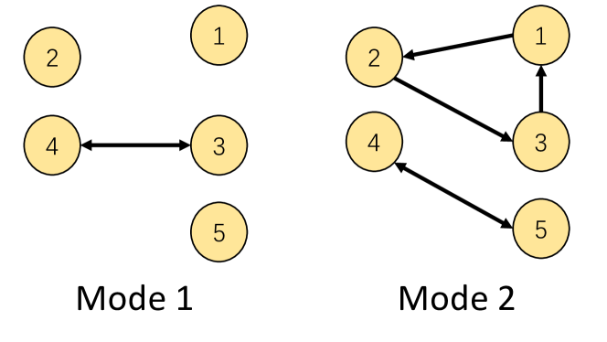
Figure 1: The communication graph is weight-balanced and switching every two seconds among the two modes.

The local objective functions are

$$\begin{array}[]{rl}f_{1}(\mathrm{x})=&\frac{1}{2}\mathrm{x}^{2}+3\mathrm{x}+1,~{}~{}f_{2}(\mathrm{x})=\frac{1}{2}\mathrm{x}^{2}-\mathrm{x},\\ f_{3}(\mathrm{x})=&\mathrm{x}^{2}+\sin{\mathrm{x}},~{}~{}f_{4}(\mathrm{x})=\ln(e^{2\mathrm{x}}+1)+0.5\mathrm{x}^{2},\\ f_{5}(\mathrm{x})=&\ln(e^{2\mathrm{x}}+e^{-0.2\mathrm{x}})+0.6\mathrm{x}^{2}.\end{array}$$

We obtain that these functions are strongly convex with $\mu_{1}=\mu_{2}=\mu_{3}=\mu_{4}=1$, $\mu_{5}=1.2$ and have Lipschitz gradient with $l_{1}=l_{2}=1$, $l_{3}=3$, $l_{4}=2$ and $l_{5}=2.41$. Let $\alpha=1$, $c_{i}=0.99$, initial conditions $x_{i}(0)\in[0,1]$, $\lambda_{i}(0)=0$, and we consider the following two cases.
Continuous-time: We obtain $\nu_{i}=-\frac{1}{\mu_{i}^{2}}$ from Lemma 1, and $0<\beta<0.5$ from Lemma 2. Choose $\beta=0.2$ and apply the continuous-time algorithm (3) under event-triggered control laws (10), (11) in MATLAB. The trajectories of $x_{i}(t)$ and triggering instants of $x_{i}$ under event-triggered communication are shown in Figure 2. It can be observed that the states converge to the optimal solution while communication is reduced due to both the jointly strongly connected graph and the event-triggered mechanism.
Discrete-time: We obtain from Lemma 3 that $\delta<0.59$. Select $\delta=0.1$, then $\tilde{\nu}_{1}=\tilde{\nu}_{2}=-1.39$, $\tilde{\nu}_{3}=-0.44$, $\tilde{\nu}_{4}=-0.59$, and $\tilde{\nu}_{5}-0.45$. $\beta$ should be less than $0.36$ according to Theorem 2. The convergence results of the discrete-time algorithm (12) under event-triggered control laws (18), (IV-B) with $\beta=0.1,0.3$ are shown in Figures 3(a) and 3(b), respectively. It can be observed that communication is greatly reduced here. We can see from (IV-B) that if other parameters are fixed, the events are triggered more frequently under a larger $\beta$. Meanwhile, $\beta$ denotes the coupling strength of agents’ states, which affects consensus speed. Thus, there exists a trade-off between the triggering instant and convergence performance, which can be observed from Figure 3.

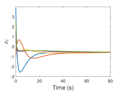
(a) The trajectories of $x_{i}(t)$.

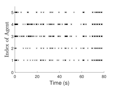
(b) triggering instant of ${x}_{i}$.

Figure 2: The trajectories of $x_{i}(t)$ and triggering instant of ${x}_{i}$ with $\beta=0.2$ for the continuous-time algorithm under event-triggered communication.

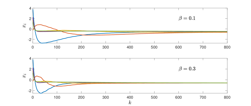
(a) The trajectories of $x_{i}(k)$.

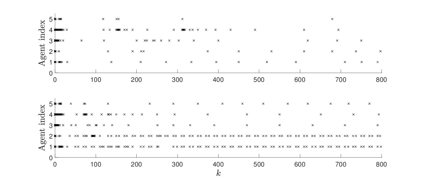
(b) Triggering instant of ${x}_{i}$ with $\beta=0.1$ in the upper and $\beta=0.3$ in the lower.

Figure 3: The trajectories of $x_{i}(k)$ and triggering instant of ${x}_{i}$ for the discrete-time algorithm under event-triggered communication.

VI Conclusion

We have proposed an event-trigger communication mechanism for the distributed continuous-time algorithm and its discrete-time counterpart over uniformly jointly strongly connected balanced graphs via the property of IFP.

References

- [1] A. Nedic, A. Olshevsky, and W. Shi, “Achieving geometric convergence for distributed optimization over time-varying graphs,” SIAM Journal on Optimization, vol. 27, no. 4, pp. 2597–2633, 2017.
- [2] P. Xie, K. You, R. Tempo, S. Song, and C. Wu, “Distributed convex optimization with inequality constraints over time-varying unbalanced digraphs,” IEEE Transactions on Automatic Control, vol. 63, no. 12, pp. 4331–4337, 2018.
- [3] H. Li, Q. Lü, and T. Huang, “Distributed projection subgradient algorithm over time-varying general unbalanced directed graphs,” IEEE Transactions on Automatic Control, vol. 64, no. 3, pp. 1309–1316, 2018.
- [4] G. Scutari and Y. Sun, “Distributed nonconvex constrained optimization over time-varying digraphs,” Mathematical Programming, vol. 176, no. 1-2, pp. 497–544, 2019.
- [5] B. Gharesifard and J. Cortés, “Distributed continuous-time convex optimization on weight-balanced digraphs,” IEEE Transactions on Automatic Control, vol. 59, no. 3, pp. 781–786, 2013.
- [6] S. S. Kia, J. Cortés, and S. Martínez, “Distributed convex optimization via continuous-time coordination algorithms with discrete-time communication,” Automatica, vol. 55, pp. 254–264, 2015.
- [7] Z. Li, Z. Ding, J. Sun, and Z. Li, “Distributed adaptive convex optimization on directed graphs via continuous-time algorithms,” IEEE Transactions on Automatic Control, vol. 63, no. 5, pp. 1434–1441, 2017.
- [8] M. Li, “Generalized Lagrange multiplier method and KKT conditions with an application to distributed optimization,” IEEE Transactions on Circuits and Systems II: Express Briefs, vol. 66, no. 2, pp. 252–256, 2019.
- [9] B. Touri and B. Gharesifard, “A modified saddle-point dynamics for distributed convex optimization on general directed graphs,” IEEE Transactions on Automatic Control, 2019.
- [10] M. Li, G. Chesi, and Y. Hong, “Input-feedforward-passivity-based distributed optimization over jointly connected balanced digraphs,” arXiv preprint arXiv:1905.03468, 2019.
- [11] S. Liu, L. Xie, and D. E. Quevedo, “Event-triggered quantized communication-based distributed convex optimization,” IEEE Transactions on Control of Network Systems, vol. 5, no. 1, pp. 167–178, 2016.
- [12] Y. Kajiyama, N. Hayashi, and S. Takai, “Distributed subgradient method with edge-based event-triggered communication,” IEEE Transactions on Automatic Control, vol. 63, no. 7, pp. 2248–2255, 2018.
- [13] C. Liu, H. Li, Y. Shi, and D. Xu, “Distributed event-triggered gradient method for constrained convex minimization,” IEEE Transactions on Automatic Control, 2019.
- [14] L. Su, M. Li, V. Gupta, and G. Chesi, “Distributed resource allocation over time-varying balanced digraphs with discrete-time communication,” arXiv preprint arXiv:1907.13003, 2019.
- [15] I. Barkana, “Defending the beauty of the invariance principle,” International Journal of Control, vol. 87, no. 1, pp. 186–206, 2014.