On the regularity of Mather’s $\beta$-function for standard-like twist maps

Abstract.

We consider the minimal average action (Mather’s $\beta$ function) for area preserving twist maps of the annulus. The regularity properties of this function share interesting relations with the dynamics of the system. We prove that the $\beta$-function associated to a standard-like twist map admits a unique $\mathscr{C}^{1}$-holomorphic complex extension, which coincides with this function on the set of real diophantine frequencies.

1. Introduction

In this note we would like to investigate some regularity properties of the so-called Mather’s $\beta$-function (or minimal average action) for twist maps of the annulus. This object is related to the minimal average action of configurations with a prescribed rotation number (the so-called Aubry-Mather orbits) and plays a crucial role in the study of the dynamics of twist maps; see section 2 for a more detailed introduction. In particular, many intriguing questions and conjectures related to problems in dynamics, analysis and geometry have been translated into questions about this function and its regularity properties (see for example [14, 21, 22, 24, 25] and references therein), shedding a new light on these issues and, in some cases, paving the way for their solution.

Two of the main questions that underpin our current interest in the subject are the following:

a) Do regularity properties of $\beta$-function (i.e. differentiability, higher smoothness, etc.) allow one to infer any information on the dynamics of the system?
b) To which extent does this function identify the system? Does it satisfy any sort of rigidity property?

Despite the huge amount of attention that these questions have attracted over the past years—in particular, understanding its regularity and its implications—they remain essentially open. In the twist map case, the best result known is that this map is strictly convex and differentiable at all irrationals. Moreover, differentiability at a rational number $p/q$ is a very atypical phenomenon: it corresponds to the existence of an invariant circle consisting of periodic orbits whose rotation number is $p/q$ (see [17]). An extension of these results to surfaces was provided in [14].

Goal of this article is to address this regularity issue and provide some new interesting answers in the special case of standard-like maps. More specifically, our starting point is the paper [4] which establishes some rigidity properties of the complex extension of analytic parametrizations of KAM curves. We use the main result of [4] to build up a $\mathscr{C}^{1}$-holomorphic complex function which coincides with Mather’s $\beta$ function on the set of real diophantine frequencies and we prove that this extension is unique. See Theorem 3 and Corollary 4 for precise statements.

The article is organized as follows. In section 2 we provide a brief introduction to Aubry-Mather theory and introduce the main object of investigation (Definition 2.2). In section 3 we state our main results (Theorem 3 and Corollary 4), whose proofs will be detailed in section 5. Some auxiliary results will be described in section 4 and appendix A.

Acknowledgements

The authors acknowledge the support of the Centro di Ricerca Matematica Ennio de Giorgi and of UniCredit Bank R$\&$D group for financial support through the Dynamics and Information Theory Institute at the Scuola Normale Superiore. CC, SM and AS acknowledge the support of MIUR PRIN Project Regular and stochastic behaviour in dynamical systems nr. 2017S35EHN. AS acknowledges the support of the MIUR Department of Excellence grant CUP E83C18000100006. DS thanks Fibonacci Laboratory for their hospitality. CC has been partially supported by the GNAMPA group of the “Istituto Nazionale di Alta Matematica” (INdAM).

2. A Synopsis of Aubry–Mather theory for twist maps of the cylinder

At the beginning of 1980s Serge Aubry and John Mather developed, independently, a novel and fruitful approach to the study of monotone twist maps of the annulus, based on the so-called principle of least action, nowadays commonly called Aubry–Mather theory. They pointed out the existence of global action-minimizing orbits for any given rotation number; these orbits minimize the discrete Lagrangian action with fixed end-points on all time intervals (for a more detailed introduction, see for example [2, 18, 21, 23]).

Let us consider the annulus ${\mathbb{S}}^{1}\times(a,b)$, where ${\mathbb{S}}^{1}:=\mathbb{R}/\mathbb{Z}$ and $a,b\in[-\infty,+\infty]$. Let us consider a diffeomorphism $f:{\mathbb{S}}^{1}\times(a,b)\longrightarrow{\mathbb{S}}^{1}\times(a,b)$ and its lift to the universal cover $\mathbb{R}\times(a,b)$, that we will continue to denote by $f$; we assume that ${f}(x+1,y)={f}(x,y)+(1,0)$ for each $(x,y)\in\mathbb{R}\times(a,b)$.

In the case in which $a,b$ are both finite, we will assume that ${f}$ extends continuously to $\mathbb{R}\times[a,b]$ and that it preserves the boundaries, with the corresponding dynamics being rotations by some fixed angles $\omega_{\pm}$:

$${f}(x,a)=(x+\omega_{-},\;a)\quad{\rm and}\quad{f}(x,b)=(x+\omega_{+},\;b).$$ (1)

For simplicity, we set $\omega_{\pm}=\pm\infty$ if $a=-\infty$ or $b=+\infty$.

Definition 2.1.

A map

$$f:\mathbb{R}\times(a,b) \longrightarrow \mathbb{R}\times(a,b)$$

$$(x_{0},y_{0}) \longmapsto (x_{1},y_{1})$$

is called a monotone twist map if:

• $f(x_{0}+1,y_{0})={f}(x_{0},y_{0})+(1,0)$;

• $f$ preserves orientation and the boundaries of $\mathbb{R}\times(a,b)$, i.e. $y_{1}(x_{0},y_{0})\xrightarrow[y_{0}\to a]{}a$ and $y_{1}(x_{0},y_{0})\xrightarrow[y_{0}\to b]{}b$ uniformly in $x_{0}$;

• if $a$ or $b$ is finite, then $f$ can be continuously extended to the boundary by a rotation, as in (1);

• $f$ satisfies the monotone twist condition

  $$\frac{\partial x_{1}}{\partial y_{0}}(x_{0},y_{0})>0\quad\text{for all $(x_{0},y_{0})\in\mathbb{R}\times(a,b)$;}$$

• $f$ is exact symplectic, i.e. there exists a function $h\colon\mathbb{R}\times\mathbb{R}\to\mathbb{R}$ such that $h(x_{0}+m,x_{1}+m)=h(x_{0},x_{1})$ for all $m\in\mathbb{Z}$ and

  $$y_{1}\,dx_{1}-y_{0}\,dx_{0}=dh(x_{0},x_{1}).$$

The interval $(\omega_{-},\omega_{+})\subset\mathbb{R}$ is then called the twist interval of $f$ and any function $h$ as above is called a generating function for $f$.

Remark.

Observe that (iv) implies that one can use $(x_{0},x_{1})$ as independent variables instead of $(x_{0},y_{0})$, namely if $(x_{1},y_{1})=f(x_{0},y_{0})$ then $y_{0}$ is uniquely determined. Moreover, the generating function $h$ allows one to reconstruct completely the dynamics of $f$; in fact, it follows from property (v) that:

$$\left\{\begin{aligned} y_{1}&=\tfrac{\partial h}{\partial x_{1}}(x_{0},x_{1})\\[4.30554pt] y_{0}&=-\tfrac{\partial h}{\partial x_{0}}(x_{0},x_{1}).\end{aligned}\right.$$ (2)

Observe that condition (iv) corresponds to asking that

$$\frac{\partial^{2}h}{\partial x_{0}\partial x_{1}}<0.$$

Examples.

• The easiest example is the following (which is an example of integrable twist map):

  $$f(x_{0},y_{0})=(x_{0}+\rho(y_{0}),y_{0}),$$

  where $\rho:(a,b)\longrightarrow\mathbb{R}$ and, in order to satisfy the twist condition, it is strictly increasing, i.e. $\rho^{\prime}(y_{0})>0$ for each $y_{0}\in(a,b)$. The dynamics is very easy: the space is foliated by a family of invariant straight lines $\{y=y_{0}\}$, on which the dynamics is a translation by $\rho(y_{0})$. Observe that if we look at the projected map on the annulus ${\mathbb{S}}^{1}\times(a,b)$, we obtain a family of invariant circles $\{y=y_{0}\}$ on which the map acts as a rotation by $\rho(y_{0}).$

  It is easy to check that a generating function is given by $h(x_{0},x_{1})=\sigma(x_{1}-x_{0})$ with any $\sigma$ such that $\sigma^{\prime}$ is the inverse bijection of $\rho$.
  

• The standard maps. One of the simplest (yet, very challenging) non-integrable twist map is the so-called standard map (this name appeared for the first time in [5]):

  $$f_{\varepsilon}(x_{0},y_{0})=(x_{1},y_{1})\enspace\text{with}\enspace\left\{\begin{aligned} x_{1}&=x_{0}+y_{0}+\varepsilon\sin(2\pi x_{0})\\ y_{1}&=y_{0}+\varepsilon\sin(2\pi x_{0})\end{aligned}\right.$$

  where $\varepsilon>0$ is a parameter ($\varepsilon=0$ would correspond to an integrable map). It is easy to check that a generating function is given by

  $$h_{\varepsilon}(x_{0},x_{1})=\frac{1}{2}(x_{1}-x_{0})^{2}-\frac{\varepsilon}{2\pi}\cos(2\pi x_{0}).$$

  This map has been the subject of extensive investigation, both from an analytical and numerical points of view. An interesting question concerns what happens in the transition between integrability and chaos; in particular, can one determine at which value of $\varepsilon$ an invariant curve of a given rotation number breaks down, or at which value there are no more invariant curves? See for example [5, 8, 9, 16, 10] (although the literature on the topics is vast).

  In section 3 we will focus on a generalized version of this map (see (5)), namely:

  $$T_{g}(x,y)=(x^{\prime},y^{\prime})\enspace\text{with}\enspace\left\{\begin{aligned} x^{\prime}&=x+y+g(x)\\ y^{\prime}&=y+g(x)\end{aligned}\right.$$

  with $g$ a 1-periodic, real analytic function of zero mean. We will refer to this kind of map as standard-like twist map.
  

• Another interesting example is provided by Birkhoff billiards. This dynamical model describes the motion of a point inside a planar strictly convex domain $\Omega$ with smooth boundary. The billiard ball moves with unit velocity and without friction following a rectilinear path; when it hits the boundary it reflects according to the standard reflection law: the angle of reflection is equal to the angle of incidence. See [26] for a more detailed introduction.

  If one considers the arc-length parametrization of the boundary $\partial\Omega$, then one can describe the billiard map as a map $B(s_{0},-\cos(\varphi_{0}))=(s_{1},-\cos(\varphi_{1}))$, where $s_{0,1}$ refer to the starting and hitting point on the boundary, while $\varphi_{0,1}\in(0,\pi)$ are the starting and hitting directions of the trajectory, with respect to the positive tangent directions on the boundary. With respect to these coordinates $(x=s,y=-\cos\varphi)$ the billiard map is a monotone twist map.
  

• Let us consider

  $$H:{\mathbb{S}}^{1}\times\mathbb{R}\times{\mathbb{S}}^{1} \longrightarrow \mathbb{R}$$

  $$(x,y,t) \longmapsto H(x,y,t),$$

  a $C^{2}$ Hamiltonian which is strictly convex and superlinear in the momentum variable (i.e. $\partial^{2}_{y}H>0$ and $\lim_{|y|\rightarrow+\infty}\frac{H(x,y)}{|y|}=+\infty$); then its time-1 map flow $\Phi_{H}^{1}:S^{1}\times\mathbb{R}\longrightarrow S^{1}\times\mathbb{R}$ can be lifted to a monotone twist map on $\mathbb{R}\times\mathbb{R}$. Such Hamiltonians are often called Tonelli Hamiltonian; see [23].

  Moser in [19] proved that every twist diffeomorphism is the time one map associated to a suitable Tonelli Hamiltonian system.
  

As follows from (2), any orbit $\{(x_{i},y_{i})\}_{i\in\mathbb{Z}}$ of the monotone twist diffeomorphism $f$ is completely determined by the sequence $(x_{i})_{i\in\mathbb{Z}}$. Moreover, this sequence corresponds to critical points of the discrete action functional:

$$\mathbb{R}^{\mathbb{Z}}\ni(x_{i})_{i\in\mathbb{Z}}\longmapsto\sum_{i\in\mathbb{Z}}h(x_{i},x_{i+1}),$$

where the series is to be interpreted as a formal object. This means that $(x_{i})_{i\in\mathbb{Z}}$ comes from an orbit of $f$ if and only if

$$\partial_{2}h(x_{i-1},x_{i})+\partial_{1}h(x_{i},x_{i+1})=0\qquad\mbox{ for all}\;i\in\mathbb{Z}$$

(hereafter we will denote by $\partial_{j}$ the derivative with respect to the $j$-th component).

Observe that while orbits correspond to critical points of the action-functional, yet they are not in general minima. Aubry-Mather theory is concerned with the study of orbits that minimize this action-functional amongst all configurations with a prescribed rotation number; we will call these orbits action-minimizing orbits or, simply, minimizers. We will call the corresponding sequences $(x_{i})_{i\in\mathbb{Z}}$ minimal configurations.

Recall that the rotation number of an orbit $\{(x_{i},y_{i})\}_{i\in\mathbb{Z}}$ is given by $\omega=\lim_{|i|\rightarrow\pm\infty}\frac{x_{i}}{|i|}$, if this limit exists. For example, in example 1 above, orbits starting at $(x_{0},y_{0})$ have rotation number $\rho(y_{0}).$ A natural question is then: does $f$ admit orbits with any prescribed rotation number? In [3], Birkhoff proved that for every rational number $p/q$ in the twist interval $(\omega_{-},\omega_{+})$, there exist at least two periodic orbits of $f$ with rotation number $p/q$.

In the eighties, Aubry [1] and Mather [15] generalised independently this result to irrational rotation numbers. More precisely:

Theorem (Aubry, Mather). A monotone twist map possesses action-minimizing orbits for every rotation number in its twist interval $(\omega_{-},\omega_{+})$.

Remark.

They also showed that every action-minimizing orbit lies on a Lipschitz graph over the $x$-axis and that if there exists an invariant circle, then every orbit on that circle is a minimizer. Hence, in the integrable case (see Example 1), each orbit is a minimizer. In a naive—yet meaningful—way, action-minimizing orbits “resemble” (and generalise) motions on invariant circles, even in the case in which invariant circles do not exist.

Two very important objects in the study of these action-minimizing orbits are represented by the so-called Mather’s minimal average actions, also called $\alpha$ and $\beta$-functions: in some sense they can be seen as an integrable Hamiltonian and Lagrangian associated to the system.

Let us now introduce the minimal average action (or Mather’s $\beta$-function) more precisely.

Definition 2.2.

Given $\omega\in(\omega_{-},\omega_{+})$, let $x^{\omega}=(x_{i})_{i\in\mathbb{Z}}$ be any minimal configuration with rotation number $\omega$. Then, the value of the minimal average action at $\omega$ is given by

$$\beta(\omega)=\lim_{\begin{subarray}{c}N_{1}\to-\infty\\ N_{2}\to+\infty\end{subarray}}\,\frac{1}{N_{2}-N_{1}}\,\sum_{i=N_{1}}^{N_{2}-1}h(x_{i},x_{i+1}).$$ (3)

This value is well-defined, since the limit exists and does not depend on the chosen orbit.

This function $\beta:(\omega_{-},\omega_{+})\longrightarrow\mathbb{R}$ encodes a lot of interesting information on the dynamical and topological properties of these action-minimizing orbits and the system. In particular, understanding whether or not this function is differentiable, or even smoother, and what are the implications of its regularity to the dynamics of the system has revealed to be a central question in the study of twist maps and, more generally, of Tonelli Hamiltonian systems (see for example [17, 14]). While for higher dimensional system this question represents a formidable problem (and is still quite far from being completely understood), in the twist-map case [17] (and for surfaces, see [14]) the situation is much more clear. In fact:

• $\beta$ is strictly convex and, hence, continuous (see [18]);

• $\beta$ is differentiable at all irrationals (see [17]);

• $\beta$ is differentiable at a rational $p/q$ if and only if there exists an invariant circle consisting of periodic aaction-minimizing orbits of rotation number $p/q$ (see [17]).
  

In particular, being $\beta$ a convex function, one can consider its convex conjugate:

$$\alpha(c)=\sup_{\omega\in\mathbb{R}}\left[\omega\,c-\beta(\omega)\right].$$

This function—which is generally called Mather’s $\alpha$-function—also plays an important rôle in the study of action-minimizing orbits and in Mather’s theory (particularly in higher dimension, see for example [14, 25]). We refer interested readers to surveys [18, 21, 23].

Observe that for each $\omega$ and $c$ one has:

$$\alpha(c)+\beta(\omega)\geq\omega c,$$

where equality is achieved if and only if $c\in\partial\beta(\omega)$ or, equivalently, if and only if $\omega\in\partial\alpha(c)$; the symbol $\partial$ denotes in this case the set of subderivatives of the function—meant as the slopes of supporting lines at a point—which is always non-empty, and is a singleton if and only if the function is differentiable at that point.

Remark.

In the billiard case, since a generating function of the billiard map is minus the Euclidean distance, $-\ell$, the action of an orbit coincides up to sign to the length of the trajectory that the ball traces on the table $\Omega$; hence, minimizing the action corresponds to maximizing the total length. Therefore, for rational numbers $-q\beta(p/q)$ represents the maximal perimeter of polygons of type $(p,q)$ (i.e. ​​, roughly speaking, polygons with $q$ vertices and winding number $p$). Moreover, it is possible to express many interesting invariants of billiards in terms of these functions (see also [22]):

• If $\Gamma_{\omega}$ is a caustic with rotation number $\omega\in(0,1/2]$, then $\beta$ is differentiable at $\omega$ and $\beta^{\prime}(\omega)=-{\rm length}(\Gamma_{\omega})=:-|\Gamma_{\omega}|$ (see [21, Theorem 3.2.10]). In particular, $\beta$ is always differentiable at $0$ and $\beta^{\prime}(0)=-|\partial\Omega|$.

• If $\Gamma_{\omega}$ is a caustic with rotation number $\omega\in(0,1/2]$, then one can associate to it another invariant, the so-called Lazutkin invariant $Q(\Gamma_{\omega})$. More precisely

  $$Q(\Gamma_{\omega})=|A-P|+|B-P|-|\stackrel{{\scriptstyle\frown}}{{AB}}|$$ (4)

  where $P$ is any point on $\partial\Omega$, $A$ and $B$ are the corresponding points on $\Gamma_{\omega}$ at which the half-lines exiting from $P$ are tangent to $\Gamma_{\omega}$ (see figure 1), and $|\cdot|$ denotes the euclidean length and $|\stackrel{{\scriptstyle\frown}}{{AB}}|$ the length of the arc on the caustic joining $A$ to $B$. This quantity is connected to the value of the $\alpha$-function (see [21, Theorem 3.2.10]):

  $$Q(\Gamma_{\omega})=\alpha(\beta^{\prime}(\omega))=\alpha(-|\Gamma_{\omega}|).\\$$

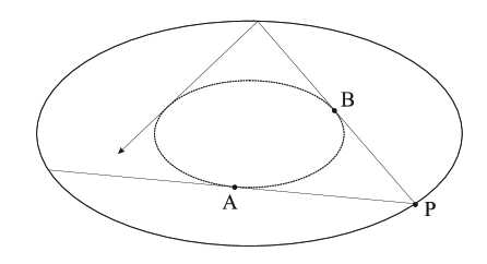
Figure 1.

Remark.

Recently, in [24], the authors drew a connection between Mather’s $\beta$-function and Fock’s function related to so-called Markov numbers; in particular, they used this relation to answer a question by Fock on the regularity of this function.

3. Statement of the main result

Let us now consider the framework of a standard-like twist map (see Example 2 in Section 2):

$$T_{g}(x,y)=(x^{\prime},y^{\prime})\enspace\text{with}\enspace\left\{\begin{aligned} x^{\prime}&=x+y+g(x)\\ y^{\prime}&=y+g(x)\end{aligned}\right.$$ (5)

with $g$ a 1-periodic, real analytic function of zero mean. Let $G$ be the primitive of $g$ with zero mean, and observe that $G$ is real analytic and 1-periodic as well. As a generating function for $T_{g}$, we take

$$h(x,x^{\prime})=\frac{1}{2}(x-x^{\prime})^{2}+G(x).$$

As was mentioned earlier, Mather’s $\beta$-function at any $\omega\in\mathbb{R}$ is defined as the average action of any minimal configuration $(x_{j})_{j\in\mathbb{Z}}$ of rotation number $\omega$:

$$\beta(\omega)=\lim_{\begin{subarray}{c}N_{1}\to-\infty\\ N_{2}\to+\infty\end{subarray}}{\,\frac{1}{N_{2}-N_{1}}}\,\sum_{N_{1}\leq j<N_{2}}h(x_{j},x_{j+1}),$$ (6)

and the general theory assures that $\beta:\mathbb{R}\to\mathbb{R}$ is continuous everywhere, and is differentiable at any $\omega\in\mathbb{R}\setminus\mathbb{Q}$. It is worth noting particular symmetry properties in the system at hand:

Lemma 1.

The function $\omega\mapsto\beta(\omega)-\frac{1}{2}\omega^{2}$ is $1$-periodic and even on $\mathbb{R}$.

Proof.

This is a consequence of the following symmetry properties of the generating function $h$:

$$h(x+m,x^{\prime}+m+1)=h(x,x^{\prime})+x^{\prime}-x+\frac{1}{2},\qquad h(x^{\prime},x)=h(x,x^{\prime})+G(x^{\prime})-G(x)$$ (7)

for all $x,x^{\prime}\in\mathbb{R}$ and $m\in\mathbb{Z}$. Indeed, take an arbitrary sequence $(x_{j})_{j\in\mathbb{Z}}$ with a definite rotation number $\omega$ and consider its finite-segment actions $A(N_{1},N_{2})\coloneqq\sum_{N_{1}\leq j<N_{2}}h(x_{j},x_{j+1})$. Setting

$$x^{*}_{j}:=x_{j}+j,\quad x^{**}_{j}:=x_{-j}\quad\text{for all $j\in\mathbb{Z}$,}$$

we get sequences with rotation numbers $\omega+1$ and $-\omega$, whose finite-segement actions can be computed from (7):

$$\sum_{N_{1}\leq j<N_{2}}h(x^{*}_{j},x^{*}_{j+1})=\sum_{N_{1}\leq j<N_{2}}[h(x_{j},x_{j+1})+x_{j+1}-x_{j}+\tfrac{1}{2}]=A(N_{1},N_{2})+x_{N_{2}}-x_{N_{1}}+\frac{N_{2}-N_{1}}{2}$$

and, changing the summation index in $\ell=-j-1$,

$$\sum_{N_{1}\leq j<N_{2}}h(x^{**}_{j},x^{**}_{j+1})=\sum_{-N_{2}-1<\ell\leq-N_{1}-1}h(x_{\ell+1},x_{\ell})=\\[4.30554pt] \sum_{-N_{2}\leq\ell<-N_{1}}[h(x_{\ell},x_{\ell+1})+G(x_{\ell+1})-G(x_{\ell})]=A(-N_{2},-N_{1})+G(x_{-N_{1}})-G(x_{-N_{2}}).$$

Hence, $(x_{j})_{j\in\mathbb{Z}}$ is a minimizer $\iff$ $(x_{j}^{*})_{j\in\mathbb{Z}}$ is a minimizer $\iff$ $(x_{j}^{**})_{j\in\mathbb{Z}}$ is a minimizer. Moreover, since $G$ is bounded, our computation entails

$$\beta(\omega+1)=\beta(\omega)+\omega+\frac{1}{2},\qquad\beta(-\omega)=\beta(\omega)$$

whence the result follows. ∎

Our main goal is to show that: if $g$ is not too large (with respect to the width of its analyticity strip), then the restriction of $\beta$ to a suitable subset of Diophantine frequencies is even more regular, in the sense that this restriction admits a $\mathscr{C}^{1}$-holomorphic extension $\beta_{{}_{\mathbb{C}}}$ defined on a complex domain (see below for the definition of $\mathscr{C}^{1}$-holomorphic functions).

In order to be more precise we need to fix some notation. Let us fix once for all $\tau>0$ and consider for $M>2\zeta(1+\tau)$ (here $\zeta$ is Riemann’s zeta function) the following Diophantine set

$$A_{M}^{\mathbb{R}}=\left\{\,\omega\in\mathbb{R}\mid\forall(n,m)\in\mathbb{Z}\times\mathbb{N}^{*},\;|\omega-\frac{n}{m}|\geq\frac{1}{Mm^{2+\tau}}\,\right\}.$$ (8)

This is a closed subset of the real line, of positive measure, which has empty interior and is invariant by the integer translations. We also consider the following subset of the complex plane

$$A_{M}^{\mathbb{C}}=\bigl{\{}\,\omega\in\mathbb{C}\mid\;\exists\omega_{*}\in A_{M}^{\mathbb{R}}\;\text{ such that }\;|\mathop{\Im m}\nolimits\omega|\geq|\omega_{*}-\mathop{\Re e}\nolimits\omega|\,\bigr{\}}$$ (9)

which has the property that $A_{M}^{\mathbb{C}}\cap\mathbb{R}=A_{M}^{\mathbb{R}}$ (see Figure 2).

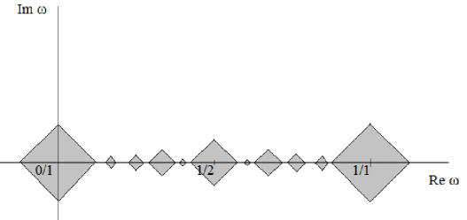
Figure 2. The perfect subset $A_{M}^{\mathbb{C}}\subset\mathbb{C}$

Many of the functions that will be important for us satisfy the periodicity condition $\varphi(\omega+1)=\varphi(\omega)$, in fact they can be even expressed as $\varphi=\psi\circ E$, where

$$E(\omega):=e^{2\pi i\omega}$$ (10)

and $\psi$ is defined on the following compact subset of the Riemann sphere $\widehat{\mathbb{C}}$ (see Figure 3):

$$K_{M}:=E(A_{M}^{\mathbb{C}})\cup\{0,\infty\}.$$ (11)

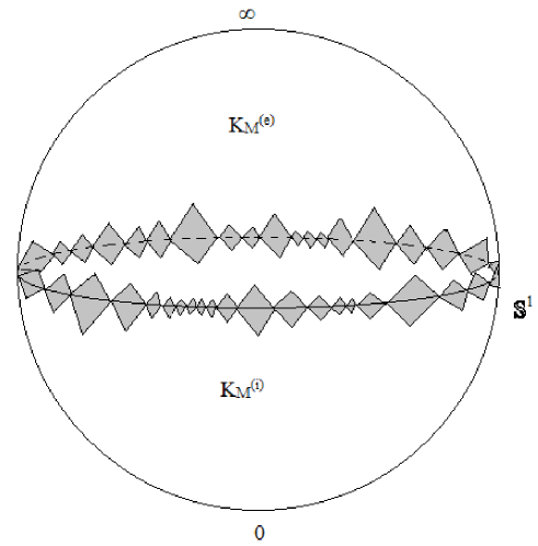
Figure 3. The perfect subset $K_{M}=K_{M}^{\textnormal{(i)}}\cup K_{M}^{\textnormal{(e)}}\subset\widehat{\mathbb{C}}$

Let us now recall the definition of the spaces of bounded $\mathscr{C}^{1}$-holomorphic functions $\mathscr{C}^{1}_{\textrm{hol}}(C,B)$, where $C\subset\mathbb{C}$ is perfect and closed and $B$ is a Banach space, and $\mathscr{C}^{1}_{\textrm{hol}}(K,B)$, where $K$ is a compact and perfect subset of $\widehat{\mathbb{C}}$. Both $\mathscr{C}^{1}_{\textrm{hol}}(C,B)$ and $\mathscr{C}^{1}_{\textrm{hol}}(K,B)$ are Banach spaces, stable under multiplication if $B$ is a Banach algebra.

The Banach space $\mathscr{C}^{1}_{\textrm{hol}}(C,B)$ and its norm are defined as follows: a function $\psi\colon C\to B$ is in $\mathscr{C}^{1}_{\textrm{hol}}(C,B)$ if it is continuous and bounded, and there is a bounded continuous function from $C$ to $B$, which we denote by $\psi^{\prime}$, such that the function $\Omega\psi\colon C\times C\to B$ defined by the formula

$$\Omega\psi(q,q^{\prime})\coloneqq\begin{dcases}\enspace\quad\psi^{\prime}(q)&\text{if $q=q^{\prime}$,}\\ \frac{\psi(q^{\prime})-\psi(q)}{q^{\prime}-q}&\text{if $q\neq q^{\prime}$,}\end{dcases}$$ (12)

is continuous and bounded; the function $\psi^{\prime}$ is then unique and we set

$$\lVert\psi\rVert_{\mathscr{C}^{1}_{\textrm{hol}}(C,B)}\coloneqq\max\Big{\{}\sup_{q\in C}\lVert\psi(q)\rVert_{B},\;\sup_{(q,q^{\prime})\in C\times C}\lVert\Omega\psi(q,q^{\prime})\rVert_{B}\Big{\}}.$$ (13)

This is a Banach space norm equivalent to the one indicated in [7] or [11] (or to the one indicated in [4], which is designed to be a Banach algebra norm whenever $B$ is a Banach algebra ).

Now, if $K$ is a compact set in $\widehat{\mathbb{C}}$, we will denote by $\mathscr{O}(K,B)$ the uniform algebra of continuous functions $\varphi\colon K\to B$ which are holomorphic in the interior of $K$, endowed with the norm

$$\lVert\varphi\rVert_{\mathscr{O}(K,B)}\coloneqq\max_{q\in K}\lVert\varphi(q)\rVert_{B}.$$ (14)

To define $\mathscr{C}^{1}_{\textrm{hol}}(K,B)$, we assume furhtermore that $K$ is perfect so as to ensure the uniqueness of the derivative. Following [6], we cover $\widehat{\mathbb{C}}$ with two charts, using $q$ as a complex coordinate in $\mathbb{C}$ and $\xi=\frac{1}{q}$ in $\widehat{\mathbb{C}}\setminus\{0\}$; a function $\varphi\colon K\to B$ belongs to $\mathscr{C}^{1}_{\textrm{hol}}(K,B)$ if its restriction $\varphi_{|K\cap\mathbb{C}}$ belongs to $\mathscr{C}^{1}_{\textrm{hol}}(K\cap\mathbb{C},B)$ and the function $\check{\varphi}\colon\xi\mapsto\varphi(1/\xi)$ belongs to $\mathscr{C}^{1}_{\textrm{hol}}(\check{K},B)$, where $\check{K}\coloneqq\{\,\xi\in\mathbb{C}\mid 1/\xi\in K\,\}$ (with the convention $1/0=\infty$), and we set

$$\lVert\varphi\rVert_{\mathscr{C}^{1}_{\textrm{hol}}(K,B)}\coloneqq\max\Big{\{}\lVert\varphi_{|K\cap\mathbb{C}}\rVert_{\mathscr{C}^{1}_{\textrm{hol}}(K\cap\mathbb{C},B)},\;\lVert\check{\varphi}\rVert_{\mathscr{C}^{1}_{\textrm{hol}}(\check{K},B)}\Big{\}},$$ (15)

As usual, we simply denote by $\mathscr{O}(K)$ and $\mathscr{C}^{1}_{\textrm{hol}}(K)$ the spaces obtained when $B=\mathbb{C}$. The following lemma, whose proof is deferred to the appendix, will be used several times:

Lemma 2.

Let $B$ be a Banach space, $A\subset\mathbb{C}$ be a closed set, and let $K$ be the closure of $E(A)$ in the Riemann sphere $\widehat{\mathbb{C}}$ with $E$ as in (10). If $\psi\in\mathscr{C}^{1}_{\textrm{hol}}(K,B)$ then the function $\psi\circ E\in\mathscr{C}^{1}_{\textrm{hol}}(A,B)$, and $\|\psi\circ E\|_{\mathscr{C}^{1}_{\textrm{hol}}(A,B)}\leq C\|\psi\|_{\mathscr{C}^{1}_{\textrm{hol}}(K,B)}$ ($C=2\pi e^{2\pi}$ will do).

We also define, for any positive real $R$,

$$S_{R}=\{z\in\mathbb{C}/\mathbb{Z}\mid|\mathop{\Im m}\nolimits z|<R\}$$ (16)

and $\|\varphi\|_{R}\coloneqq\sup_{z\in S_{R}}|\varphi(z)|$ for any function $\varphi\colon S_{R}\to\mathbb{C}$. Our main result is:

Theorem 3.

Let $R_{1}$ be positive real. Then there is $c=c(\tau,R_{1})>0$ such that, for any real analytic 1-periodic function $g$ which has zero mean and extends holomorphically to $S_{R_{1}}$ with $\|g\|_{R_{1}}<c$, and for any $M$ such that $1<\frac{M}{2\zeta(1+\tau)}<\big{(}\frac{c}{\|g\|_{R_{1}}}\big{)}^{1/8}$, Mather’s $\beta$-function for the system (5) satisfies the following: $\beta|_{A_{M}^{\mathbb{R}}}$ admits a complex extension to $A_{M}^{\mathbb{C}}$ of the form

$$\beta_{{}_{\mathbb{C}}}(\omega)\coloneqq\frac{\omega^{2}}{2}+\Phi^{\mathbb{C}}_{\beta}(\omega),$$

where $\Phi^{\mathbb{C}}_{\beta}\in\mathscr{C}^{1}_{\textrm{hol}}(A_{M}^{\mathbb{C}})$. Moreover,

• the derivative of $\beta_{{}_{\mathbb{C}}}$ is an extension of the derivative of $\beta|_{A_{M}^{\mathbb{R}}}$;

• the function $\Phi_{\beta}^{\mathbb{C}}$ is even and 1-periodic, and $\overline{\Phi^{\mathbb{C}}_{\beta}(\omega)}=\Phi^{\mathbb{C}}_{\beta}(\overline{\omega})$;

• $\Phi^{\mathbb{C}}_{\beta}=\tilde{\Phi}\circ E$ for a function $\tilde{\Phi}\in\mathscr{C}^{1}_{\textrm{hol}}(K_{M})$ and $E(z):=e^{2\pi iz}$. This implies that $\Phi^{\mathbb{C}}_{\beta}$ is defined in an infinite strip $\{\mathop{\Im m}\nolimits\omega>\ell\}$ (resp. $\{\mathop{\Im m}\nolimits\omega<-\ell\}$) and admits a limit as $\mathop{\Im m}\nolimits\omega\to+\infty$ (resp. $\mathop{\Im m}\nolimits\omega\to-\infty$).

We thus have

$$\beta_{{}_{\mathbb{C}}}|_{A_{M}^{\mathbb{R}}}=\beta|_{A_{M}^{\mathbb{R}}},\qquad\beta_{{}_{\mathbb{C}}}^{\prime}|_{A_{M}^{\mathbb{R}}}=\beta^{\prime}|_{A_{M}^{\mathbb{R}}}.$$

We may refer to $\beta_{{}_{\mathbb{C}}}$ as a $\mathscr{C}^{1}_{\textrm{hol}}$-holomorphic function, but notice that $\beta_{{}_{\mathbb{C}}}$ is not bounded, it is $\beta_{{}_{\mathbb{C}}}(\omega)-\frac{\omega^{2}}{2}$ that belongs to $\mathscr{C}^{1}_{\textrm{hol}}(A_{M}^{\mathbb{C}})$.

The proof of Theorem 3 is given in Sections 4–5. It relies on a result of [4], which studies regularity properties of the parametrized KAM curves: the result on the beta function will be obtained by averaging on the these curves, as we explain below.

The extension $\beta_{{}_{\mathbb{C}}}$ of $\beta|_{A_{M}^{\mathbb{R}}}$ provided by Theorem 3 is unique and does not depend on $M$. This follows from the quasi-analyticity property established in [12], according to which the space of functions $\mathscr{C}^{1}_{\textrm{hol}}(A^{\mathbb{C}}_{M})$ is $\mathscr{H}^{1}$-quasi-analytic, where $\mathscr{H}^{1}$ denotes the $1$-dimensional Hausdorff measure : any subset $\Omega\subset A^{\mathbb{C}}_{M}$ of positive $\mathscr{H}^{1}$-measure is a uniqueness set for this space of functions.

This quasi-analyticity property has the following striking consequence on the real Mather’s $\beta$-function:

Corollary 4.

Let $R_{1}>0$ and let $g$ be real analytic 1-periodic, which has zero mean and extends holomorphically to $S_{R_{1}}$ so that $\|g\|_{R_{1}}<c/3$, with $c=c(\tau,R_{1})$ as in Theorem 3. Then there exists $M>2\zeta(1+\tau)$ such that, for every $\omega_{0}\in\mathbb{R}$, the function $\beta|_{A^{\mathbb{R}}_{M}}$ is determined by the restriction of $\beta$ to any subset of $[\omega_{0},\omega_{0}+1]$ of Lebesgue measure $\geq\big{(}\frac{3\|g\|_{R_{1}}}{c}\big{)}^{1/8}$. One can take $M\coloneqq 2\zeta(1+\tau)\big{(}\frac{c}{2\|g\|_{R_{1}}}\big{)}^{1/8}$.

Proof of Corollary 4.

Since $\|g\|_{R_{1}}<c/3$, we get

$$1<\big{(}\tfrac{c}{3\|g\|_{R_{1}}}\big{)}^{1/8}<\tfrac{M}{2\zeta(1+\tau)}<\big{(}\tfrac{c}{\|g\|_{R_{1}}}\big{)}^{1/8}$$

and we can apply Theorem 3. We get a function $\beta_{{}_{\mathbb{C}}}(\omega)=\frac{\omega^{2}}{2}+\Phi^{\mathbb{C}}_{\beta}(\omega)$ with $\Phi^{\mathbb{C}}_{\beta}\in\mathscr{C}^{1}_{\textrm{hol}}(A^{\mathbb{C}}_{M})$.

Let us denote by $m$ the Lebesgue measure on $\mathbb{R}$. Let $\Omega\subset[\omega_{0},\omega_{0}+1]$ have $m(\Omega)\geq\big{(}\frac{3\|g\|_{R_{1}}}{c}\big{)}^{1/8}$. We will prove that $\Omega\cap A^{\mathbb{R}}_{M}$ is a uniqueness set for $\mathscr{C}^{1}_{\textrm{hol}}(A^{\mathbb{C}}_{M})$.

As is well known, $m\big{(}[\omega_{0},\omega_{0}+1]\setminus A^{\mathbb{R}}_{M}\big{)}<2\zeta(1+\tau)/M$, hence

$$m\big{(}[\omega_{0},\omega_{0}+1]\setminus A^{\mathbb{R}}_{M}\big{)}<\big{(}\tfrac{2\|g\|_{R_{1}}}{c}\big{)}^{1/8}<m(\Omega).$$

Consequently, $m(\Omega\cap A^{\mathbb{R}}_{M})=m(\Omega)-m\big{(}\Omega\cap([\omega_{0},\omega_{0}+1]\setminus A^{\mathbb{R}}_{M})\big{)}>0$ and $\Omega\cap A^{\mathbb{R}}_{M}$ is thus a uniqueness set for $\mathscr{C}^{1}_{\textrm{hol}}(A^{\mathbb{C}}_{M})$. It follows that $\Phi^{\mathbb{C}}_{\beta}$ is determined by ${\Phi^{\mathbb{C}}_{\beta}}_{|\Omega\cap A^{\mathbb{R}}_{M}}$; hence $\beta_{{}_{\mathbb{C}}}$, and also $\beta|_{A^{\mathbb{R}}_{M}}=\beta_{{}_{\mathbb{C}}}|_{A^{\mathbb{R}}_{M}}$, are determined by $\beta|_{\Omega\cap A^{\mathbb{R}}_{M}}$. ∎

4. Intermediate results

In order to prove Theorem 3, let us first recall part of the results of [4].

A parametrized invariant curve of rotation number $\omega$ for $T_{g}$ is a pair of continuous functions $(U,V):\mathbb{T}\to\mathbb{T}\times\mathbb{R}$ such that

$$T_{g}(U(\theta),V(\theta))=(U(\theta+\omega),V(\theta+\omega))\enspace\text{for all $\theta\in\mathbb{T}$.}$$ (17)

Note that, if $(U,V)$ is a parametrized invariant curve for $T_{g}$ of rotation number $\omega\in\mathbb{R}\setminus\mathbb{Q}$, then $(U(j\omega))_{j\in\mathbb{Z}}$ is a minimal configuration of rotation number $\omega$ and the limit in equation (6) becomes

$$\beta(\omega)=\lim_{\begin{subarray}{c}N_{1}\to-\infty\\ N_{2}\to+\infty\end{subarray}}\,\frac{1}{N_{2}-N_{1}}\,\sum_{N_{1}\leq j<N_{2}}\Big{[}\frac{1}{2}\left\lvert V\big{(}(j+1)\omega\big{)}\right\rvert^{2}+G(U(j\omega))\Big{]}\\ =\frac{1}{2}\int_{\mathbb{T}}|V(\theta)|^{2}d\theta+\int_{\mathbb{T}}G(U(\theta))d\theta,$$ (18)

where we have used Birkhoff’s ergodic theorem for the (uniquely) ergodic rotation of angle $\omega\in\mathbb{R}\setminus\mathbb{Q}$ on $\mathbb{T}$.

Since we will be interested in a perturbative result (i.e. valid for $\|g\|_{R_{0}}$ small), it is natural to write $U(\theta)=\theta+u(\theta)$, $V(\theta)=\omega+v(\theta)$. Taking into account the fact that equation (5) implies $x^{\prime}-x=y^{\prime}$, we can reduce the quest of an invariant curve to the solution of the following system of equations:

$$\left\{\begin{aligned} &u(\theta+\omega)-2u(\theta)+u(\theta-\omega)=g\big{(}\theta+u(\theta)\big{)}\\ &v(\theta)=u(\theta)-u(\theta-\omega).\end{aligned}\right.$$ (19)

It is in fact sufficient to solve the first equation for $u$: any $1$-periodic solution $u$ to this second-order difference equation is the first component of an invariant curve of frequency $\omega$.

Let us denote by $H^{\infty}(S_{R})$ the Banach space of 1-periodic bounded holomorphic functions on $S_{R}$ endowed with the supremum norm $\|\,.\,\|_{R}$. The approach of [4] considers the unknown $u=u(\theta,\omega)$ in equation (19a) as a function of two complex variables, the angle $\theta\in S_{R}$ and the frequency $\omega\in A^{\mathbb{C}}_{M}$, or more precisely as a function of $\omega\in A^{\mathbb{C}}_{M}$ with values in $H^{\infty}(S_{R})$. We quote the result as follows:

Theorem 5 (Theorem 1, [4]).

Suppose $0<R<R_{0}$ and $K>0$. Then there is $c_{0}=c_{0}(\tau,K,R,R_{0})$ such that for any $f\colon\mathbb{R}\to\mathbb{R}$ 1-periodic with zero mean which extends holomorphically to a neighbourhood of $\overline{S_{R_{0}}}$ with $\max\{\|f\|_{R_{0}},\|f^{\prime\prime}\|_{R_{0}}\}\leq K$, for all $M>2\zeta(1+\tau)$, and for all positive $\varepsilon<c_{0}M^{-8}$, there exists $\tilde{u}=\tilde{u}_{\varepsilon,M}\in\mathscr{C}^{1}_{\textrm{hol}}(K_{M},H^{\infty}(S_{R}))$ with zero mean such that $u:=\tilde{u}\circ E$ (where $E(z):=e^{2\pi iz}$) satisfies

$$u(\theta+\omega,\omega)-2u(\theta,\omega)+u(\theta-\omega,\omega)=\varepsilon f\big{(}\theta+u(\theta,\omega)\big{)}$$ (20)

for all $\theta\in S_{R}$ and $\omega\in A^{\mathbb{C}}_{M}$ such that $\theta\pm\omega\in S_{R}$, and $u(\theta,\omega)\in\mathbb{R}$ if $\theta\in\mathbb{R}/\mathbb{Z}$ and $\omega\in A^{\mathbb{R}}_{M}$. Moreover $\|\tilde{u}\|_{\mathscr{C}^{1}_{\textrm{hol}}(K_{M},H^{\infty}(S_{R}))}\leq\frac{R_{0}-R}{4}$.

Remark.

Actually the statement above differs from the one in [4] for a couple of minor aspects. Indeed, in [4] the function $\tilde{u}$ is thought as an element of the space $\mathscr{C}^{1}_{\textrm{hol}}(A^{\mathbb{C}}_{M},H^{\infty}(S_{R}\times\mathbb{D}_{\rho}))$, with $\rho=c_{0}M^{-8}$, while here we are only using the result for fixed $\varepsilon$.

Moreover in the statement of Theorem 1 in [4] the constant $c_{0}$ depends on $f$. However, analysing the proof one realizes that, for the iterative scheme to work, the constant $c_{0}$ can be determined only in terms of $\|f\|_{R_{0}}$ and $\|f^{\prime\prime}\|_{R_{0}}$, and does not actually depend on the specific choice of $f$ (see in particular the remark in [4] on p. 2053, a few lines before § 4.2). The last estimate in Theorem 5 does not appear in the statement in [4], but is a by-product of the proof of Lemma 19 in [4], on p. 2057.

Let us rephrase the result getting rid of the parameter $\varepsilon$:

Corollary 6.

Suppose $0<R<R_{1}$. Then there is $c_{1}=c_{1}(\tau,R,R_{1})$ such that for any $M>2\zeta(1+\tau)$, and for any $g:\mathbb{R}\to\mathbb{R}$ 1-periodic with zero mean which extends holomorphically to a neighbourhood of $\overline{S_{R_{1}}}$ with $\|g\|_{R_{1}}<c_{1}M^{-8}$, there exists $\tilde{u}=\tilde{u}_{M}\in\mathscr{C}^{1}_{\textrm{hol}}(K_{M},H^{\infty}(S_{R}))$ with zero mean, such that $u:=\tilde{u}\circ E$ (where $E(\omega):=e^{2\pi i\omega}$) satisfies

$$u(\theta+\omega,\omega)-2u(\theta,\omega)+u(\theta-\omega,\omega)=g\big{(}\theta+u(\theta),\omega\big{)}$$ (21)

for all $\theta\in S_{R}$ and $\omega\in A^{\mathbb{C}}_{M}$ such that $\theta\pm\omega\in S_{R}$, and $u(\theta,\omega)\in\mathbb{R}$ if $\theta\in\mathbb{R}/\mathbb{Z}$ and $\omega\in A^{\mathbb{R}}_{M}$.

Proof.

Let $R_{0}:=\frac{R_{1}+R}{2}$ and $K:=\max\{1,\frac{2}{\pi(R_{0}-R)^{2}}\}$. Cauchy inequalities yield $\|g^{\prime\prime}\|_{R_{0}}\leq\frac{2}{\pi(R_{0}-R)^{2}}\|g\|_{R_{1}}$, therefore

$$\max\{\|g\|_{R_{0}},\|g^{\prime\prime}\|_{R_{0}}\}\leq K\|g\|_{R_{1}}.$$

Let us set $c_{1}:=c_{0}/2$ (for $c_{0}=c_{0}(\tau,K,R,R_{0})$ as in Theorem 5), and note that $f:=\frac{M^{8}}{c_{1}}g$ is such that

$$\max\{\|f\|_{R_{0}},\|f^{\prime\prime}\|_{R_{0}}\}\leq\frac{M^{8}}{c_{1}}\max\{\|g\|_{R_{0}},\|g^{\prime\prime}\|_{R_{0}}\}\leq\frac{M^{8}}{c_{1}}K\|g\|_{R_{1}}\leq K.$$

Therefore, choosing $\varepsilon=c_{1}M^{-8}$ and $g=\varepsilon f$, Corollary 6 immediately follows from Theorem 5. ∎

Remark.

From the definition of the function spaces in [4] we deduce that not only $\tilde{u}\in\mathscr{C}^{1}_{\textrm{hol}}(K_{M},H^{\infty}(S_{R}))$, but $\tilde{u}$ admits a normally convergent Fourier expansion

$$\tilde{u}(q,\cdot)=\sum_{k}\hat{u}_{k}(q)e_{k}\ \ \mbox{ with }\ \ \ \begin{cases}\hat{u}_{k}\in\mathscr{C}^{1}_{\textrm{hol}}(K_{M})\\ e_{k}(\theta):=e^{2\pi ik\theta}\end{cases}$$ (22)

Moreover (cf. [4], Definition 3.2) also

$$\sum_{k}q^{k}\hat{u}_{k}(q)e_{k}\ \ \mbox{ and }\ \ \sum_{k}q^{-k}\hat{u}_{k}(q)e_{k}$$ (23)

converge normally in $\mathscr{C}^{1}_{\textrm{hol}}(K_{M},H^{\infty}(S_{R}))$ and (cf. [4], Definition 3.3)

$$\overline{\hat{u}_{k}(q)}=\hat{u}_{-k}(1/\overline{q})$$ (24)

Lemma 7.

The function $u=\tilde{u}\circ E$ of Corollary 6 is $1$-periodic in $\omega$, it belongs to the space $\mathscr{C}^{1}_{\textrm{hol}}(A^{\mathbb{C}}_{M},H^{\infty}(S_{R}))$, and it satisfies

$$u(\theta,-\omega)=u(\theta,\omega),\qquad\overline{u(\theta,\omega)}=u(\overline{\theta},\overline{\omega}).$$

Proof.

The periodicity of $u$ follows from the periodicity of $E(\omega)=e^{2\pi i\omega}$ and its $\mathscr{C}^{1}$-holomorphy from Lemma 2. By construction, $\omega\in A^{\mathbb{C}}_{M}\iff-\omega\in A^{\mathbb{C}}_{M}$, so setting $u^{*}(\theta,\omega)\coloneqq u(\theta,-\omega)$, it is easy to check that $u^{*}\in\mathscr{C}^{1}_{\textrm{hol}}(A^{\mathbb{C}}_{M},H^{\infty}(S_{R}))$. Now, $u^{*}$ is clearly a solution to (19). Thus, by the uniqueness argument of [4] (see footnote 6 on p. 2038), we get $u_{|A^{\mathbb{R}}_{M}}=u^{*}_{|A^{\mathbb{R}}_{M}}$, hence, by the quasi-analyticity argument of [12], $u=u^{*}$. From (24), it follows that $\overline{u(\theta,\omega)}=u(\overline{\theta},\overline{\omega})$. ∎

5. Proof of Theorem 3

We now give ourselves $R_{1}>0$ and define $c\coloneqq\big{(}2\zeta(1+\tau)\big{)}^{-8}c_{1}$, with $R\coloneqq R_{1}/2$ and $c_{1}=c_{1}(\tau,R,R_{1})$ as in Corollary 6. We suppose that $g$ and $M$ satisfy the assumptions of Theorem 3 with this value of $c$. We must find a function $\beta_{{}_{\mathbb{C}}}$ satisfying all the claims of Theorem 3.

Among our assumptions, we have $1<\frac{M}{2\zeta(1+\tau)}<\big{(}\frac{c}{\|g\|_{R_{1}}}\big{)}^{1/8}$, therefore $M>2\zeta(1+\tau)$ and $\frac{\|g\|_{R_{1}}}{c}<\big{(}2\zeta(1+\tau)\big{)}^{8}M^{-8}$, whence $\|g\|_{R_{1}}<c_{1}M^{-8}$. We can thus apply Corollary 6 and use the function $u=\tilde{u}\circ E$ satisfying equation (21) as well as the properties described in Lemma 7.

From now on, if $\tilde{\varphi}\in\mathscr{C}^{1}_{\textrm{hol}}(K_{M},H^{\infty}(S_{r}))$ has Fourier expansion $\tilde{\varphi}(\theta,q)=\sum_{k}\hat{\varphi}_{k}(q)e_{k}(\theta)$ we define

$$\tilde{\varphi}^{\pm}(\theta,q)=\sum_{k}q^{\pm k}\hat{\varphi}_{k}(q)e_{k}(\theta).$$

Note that, by (23), $\tilde{u}^{\pm}$ both belong to $\mathscr{C}^{1}_{\textrm{hol}}(K_{M},H^{\infty}(S_{r}))$. Moreover, if $\varphi:=\tilde{\varphi}\circ E\in\mathscr{C}^{1}_{\textrm{hol}}(A^{\mathbb{C}}_{M},H^{\infty}(S_{r}))$, by a slight abuse of notation we denote by $\varphi^{\pm}=\tilde{\varphi}^{\pm}\circ E$, which boils down to $\varphi^{\pm}(\theta,\omega)=\varphi(\theta\pm\omega,\omega)$. Moreover we set

$$v\coloneqq u-u^{-},\quad U(\theta,\omega)\coloneqq\theta+u(\theta,\omega),\quad V(\theta,\omega)\coloneqq\omega+v(\theta,\omega).$$

Since $\tilde{u}^{\pm}\in\mathscr{C}^{1}_{\textrm{hol}}(K_{M},H^{\infty}(S_{r}))$ we get that $u^{\pm}$ both belong to $\mathscr{C}^{1}_{\textrm{hol}}(A^{\mathbb{C}}_{M},H^{\infty}(S_{r}))$, and the same is true for $v$.

Lemma 8.

The formula

$$\begin{split}\beta_{{}_{\mathbb{C}}}(\omega)&:=\int_{0}^{1}\Big{[}\frac{1}{2}V(\theta,\omega)^{2}+G\big{(}U(\theta,\omega)\big{)}\Big{]}d\theta\\ &=\frac{1}{2}\omega^{2}+\int_{0}^{1}\Big{[}\frac{1}{2}v(\theta,\omega)^{2}+G(\theta+u(\theta,\omega))\Big{]}d\theta\end{split}$$ (25)

defines a function $\beta_{{}_{\mathbb{C}}}$ which can be written in the form $\beta_{{}_{\mathbb{C}}}(\omega)=\frac{\omega^{2}}{2}+\Phi_{\beta}^{\mathbb{C}}(\omega)$ with $\Phi_{\beta}^{\mathbb{C}}\in\mathscr{C}^{1}_{\textrm{hol}}(A^{\mathbb{C}}_{M})$; in fact, $\Phi_{\beta}^{\mathbb{C}}=\tilde{\Phi}\circ E$ with $\tilde{\Phi}\in\mathscr{C}^{1}_{\textrm{hol}}(K_{M})$. Moreover,

$$\frac{d\beta_{{}_{\mathbb{C}}}}{d\omega}=\int_{0}^{1}V(\theta,\omega)\partial_{\theta}U(\theta,\omega)d\theta=\omega+\int_{0}^{1}v(\theta,\omega)\partial_{\theta}u(\theta,\omega)d\theta.$$ (26)

Proof.

By periodicity of $u$ we immediately get that $\int_{0}^{1}vd\theta=0$, $\int_{0}^{1}Vd\theta=\omega$, so the two expressions for $\beta_{{}_{\mathbb{C}}}$ above are equivalent.

The fact that

$$\Phi_{\beta}^{\mathbb{C}}(\omega)\coloneqq\beta_{{}_{\mathbb{C}}}(\omega)-\frac{\omega^{2}}{2}=\int_{0}^{1}\Big{[}\frac{1}{2}v(\theta,\omega)^{2}+G(\theta+u(\theta,\omega))\Big{]}d\theta$$ (27)

belongs to $\mathscr{C}^{1}_{\textrm{hol}}(A^{\mathbb{C}}_{M})$ is a consequence of the results in [4]. Indeed, since $v\in\mathscr{C}^{1}_{\textrm{hol}}(A^{\mathbb{C}}_{M},H^{\infty}(S_{r}))$, its square also belongs to that space, and Lemma 11 of [4] ensures that

$$G\circ(id+\tilde{u})\in\mathscr{C}^{1}_{\textrm{hol}}(K_{M},H^{\infty}(S_{R})),$$ (28)

hence, by Lemma 2, $G\circ(id+u)=G\circ(id+\tilde{u})\circ E\in\mathscr{C}^{1}_{\textrm{hol}}(A^{\mathbb{C}}_{M},H^{\infty}(S_{R}))$. On the other hand, Lemma 4 of [4] ensures that if

$$\varphi\in\mathscr{C}^{1}_{\textrm{hol}}(A^{\mathbb{C}}_{M},H^{\infty}(S_{R}))\quad\Longrightarrow\quad[\omega\mapsto\int_{0}^{1}\varphi(\theta,\omega)d\theta]\in\mathscr{C}^{1}_{\textrm{hol}}(A^{\mathbb{C}}_{M}).$$ (29)

Now we can write

$$\beta_{{}_{\mathbb{C}}}(\omega)=\int_{0}^{1}\frac{1}{2}V^{2}d\theta+\int_{0}^{1}G\circ Ud\theta=\int_{0}^{1}\frac{1}{2}(V^{+})^{2}d\theta+\int_{0}^{1}G\circ Ud\theta$$

thus

$$\frac{d\beta_{{}_{\mathbb{C}}}}{d\omega}=\int_{0}^{1}V^{+}\partial_{\omega}V^{+}d\theta+\int_{0}^{1}(g\circ U)\partial_{\omega}Ud\theta.$$ (30)

Since $V^{+}(\theta,\omega)=U(\theta+\omega,\omega)-U(\theta,\omega)$ we get that

$$\partial_{\omega}V^{+}=(\partial_{\theta}U)^{+}+(\partial_{\omega}U)^{+}-\partial_{\omega}U$$ (31)

Moreover by (21) we get that $g\circ U=u^{+}-2u+u^{-}=V^{+}-V$ so that

$$\int_{0}^{1}(g\circ U)\partial_{\omega}Ud\theta=\int_{0}^{1}(V^{+}-V)\partial_{\omega}Ud\theta$$ (32)

thus

$$\begin{split}\frac{d\tilde{\beta}}{d\omega}&=\int_{0}^{1}V^{+}(\partial_{\theta}U)^{+}d\theta+\int_{0}^{1}V^{+}[(\partial_{\omega}U)^{+}-\partial_{\omega}U]d\theta+\int_{0}^{1}(g\circ U)\partial_{\omega}Ud\theta\\ &=\int_{0}^{1}V^{+}(\partial_{\theta}U)^{+}d\theta=\int_{0}^{1}V\partial_{\theta}Ud\theta\end{split}$$ (33)

where the first equality follows from equation (31) while equation (32) allows us to pass from the first line to the second; and translation invariance has been used several times as well.

We have $\Phi_{\beta}^{\mathbb{C}}=\tilde{\Phi}\circ E$ with

$$\tilde{\Phi}(q):=\int_{0}^{1}\Big{[}\frac{1}{2}\big{(}\tilde{u}(\theta,q)-\tilde{u}^{-}(\theta,q)\big{)}^{2}+G\big{(}\theta+\tilde{u}(\theta,q)\big{)}\Big{]}d\theta.$$ (34)

Using $\tilde{u},\tilde{u}^{-}\in\mathscr{C}^{1}_{\textrm{hol}}(K_{M},H^{\infty}(S_{R}))$, the stability of this space under multiplication, and (28)–(29), we obtain $\tilde{\Phi}\in\mathscr{C}^{1}_{\textrm{hol}}(K_{M})$. ∎

Proposition 9.

The function $\beta_{{}_{\mathbb{C}}}$ defined in Lemma 8 coincides with Mather’s $\beta$-function on the real line. In fact,

$$(i)\ \beta_{{}_{\mathbb{C}}}|_{A^{\mathbb{R}}_{M}}=\beta|_{A^{\mathbb{R}}_{M}}\qquad(ii)\ \beta_{{}_{\mathbb{C}}}^{\prime}|_{A^{\mathbb{R}}_{M}}=\beta^{\prime}|_{A^{\mathbb{R}}_{M}}$$ (35)

Proof.

For $\omega\in A^{\mathbb{R}}_{M}$ the sequence $x_{j}:=U(j\omega,\omega)$ defines a minimal configuration $(x_{j})_{j\in\mathbb{Z}}$ with rotation number $\omega$; in fact, setting $y_{j}:=\omega+V(j\omega,\omega)$ yields $T(x_{j},y_{j})=(x_{j+1},y_{j+1})$. The proof of (i) then follows from equation (18).

The proof of (ii) follows from a well known formula (see [21], Theorem 1.3.7-(4)) which expresses the derivative of Mather’s $\beta$-function in terms of $U$ and $V$:

$$\beta^{\prime}(\omega)=\int_{0}^{1}V(\theta,\omega)\partial_{\theta}U(\theta,\omega)d\theta$$

Thus $\beta^{\prime}(\omega)=\beta_{{}_{\mathbb{C}}}^{\prime}(\omega)$ by equation (26). ∎

At this stage, only point (ii) of Theorem 3 remains to be proved. According to Lemma 7, we have

$$u(\theta,-\omega)=u(\theta,\omega)=u(\theta,\omega+1)=\overline{u(\overline{\theta},\overline{\omega})}.$$

This implies

$$v(\theta,-\omega)=u(\theta,-\omega)-u(\theta+\omega,-\omega)=u(\theta,\omega)-u(\theta+\omega,\omega)=-v(\theta+\omega,\omega)$$

and $v(\theta,\omega+1)=v(\theta,\omega)=\overline{v(\overline{\theta},\overline{\omega})}$. In view of (27), this yields

$$\Phi^{\mathbb{C}}_{\beta}(-\omega)=\Phi^{\mathbb{C}}_{\beta}(\omega)=\Phi^{\mathbb{C}}_{\beta}(\omega+1)=\overline{\Phi^{\mathbb{C}}_{\beta}(\overline{\omega})}$$

and we are done.

Appendix A Proof of Lemma 2

Let $\psi\in{\mathscr{C}^{1}_{\textrm{hol}}(K,B)}$. We use the same notations for $\check{K}$ and $\check{\psi}$ as in the definition of the space ${\mathscr{C}^{1}_{\textrm{hol}}(K,B)}$ given in Section 3. Notice that

$$K\cap\mathbb{C}=E(A)\enspace\text{or}\enspace E(A)\cup\{0\},\qquad\check{K}=E(-A)\enspace\text{or}\enspace E(-A)\cup\{0\}$$

according as $\inf\{Re\,\omega\mid\omega\in A\}>-\infty$ or not for the former, and $\sup\{Re\,\omega\mid\omega\in A\}<+\infty$ or not for the latter.

Let $\varphi\coloneqq\psi\circ E$. Clearly, $\varphi$ is bounded and $\displaystyle\sup_{\omega\in A}\lVert\varphi(\omega)\rVert_{B}\leq\sup_{q\in K}\lVert\psi(q)\rVert_{B}\leq\lVert\psi\rVert_{\mathscr{C}^{1}_{\textrm{hol}}(K,B)}$. For $(\omega,\omega^{\prime})\in A\times A$ with $\omega\neq\omega^{\prime}$, we have

$$\Omega\varphi(\omega,\omega^{\prime})=\frac{\psi(q^{\prime})-\psi(q)}{q^{\prime}-q}\frac{q^{\prime}-q}{\omega^{\prime}-\omega}=\frac{\check{\psi}(\xi^{\prime})-\check{\psi}(\xi)}{\xi^{\prime}-\xi}\frac{\xi^{\prime}-\xi}{\omega^{\prime}-\omega}$$ (36)

with $q\coloneqq E(\omega)$, $q^{\prime}\coloneqq E(\omega^{\prime})$, $\xi\coloneqq E(-\omega)$, $\xi^{\prime}\coloneqq E(-\omega^{\prime})$. Letting $\omega^{\prime}$ tend to $\omega$, we get

$$2\pi iE(\omega)\psi^{\prime}(E(\omega))=-2\pi iE(-\omega)\check{\psi}^{\prime}(E(-\omega))$$

and we define both $\Omega\varphi(\omega,\omega)$ and $\varphi^{\prime}(\omega)$ as this common value. This way $\Omega\varphi$ is continuous on $A\times A$.

Let us write $A=A^{+}\cup A^{-}$, where $A^{\pm}$ are the overlapping regions

$$A^{+}\coloneqq\{\omega\in A\mid\mathop{\Im m}\nolimits\omega>-1\},\qquad A^{-}\coloneqq\{\omega\in A\mid\mathop{\Im m}\nolimits\omega<1\}.$$

If both $\omega$ and $\omega^{\prime}$ belong to $A^{+}$ (resp. $A^{-}$), then the quantity $|\frac{q^{\prime}-q}{\omega^{\prime}-\omega}|$ (resp. $|\frac{\xi^{\prime}-\xi}{\omega^{\prime}-\omega}|$) is bounded by $2\pi e^{2\pi}$, hence by the first (resp. second) expression in (36) we get

$$\lVert\Omega\varphi(\omega,\omega^{\prime})\rVert_{B}\leq 2\pi e^{2\pi}\lVert\psi\rVert_{\mathscr{C}^{1}_{\textrm{hol}}(K,B)},$$ (37)

and also $\lVert\varphi^{\prime}(\omega)\rVert_{B}\leq 2\pi e^{2\pi}\lVert\psi\rVert_{\mathscr{C}^{1}_{\textrm{hol}}(K,B)}$ by continuity. If $\omega$ and $\omega^{\prime}$ do not lie in the same region, then $|\omega-\omega^{\prime}|\geq 2$, hence $\lVert\Omega\varphi(\omega,\omega^{\prime})\rVert_{B}=\lVert\frac{\psi(q^{\prime})-\psi(q)}{\omega^{\prime}-\omega}\rVert_{B}\leq\lVert\psi\rVert_{\mathscr{C}^{1}_{\textrm{hol}}(K,B)}$.

Therefore, (37) always holds true, which completes the proof of our claim.

References

[1]
Sergey Aubry.
The twist map, the extended Frenkel–Kontorova model and the devil’s staircase.
Physica, 7D: 240–258, 1983.
[2]
Victor Bangert.
Mather sets for twist maps and geodesics on tori.
Dynamics reported Ser. Dynam. Systems Appl., Vol. 1, 1–56, 1988.
[3]
George D. Birkhoff.
Surface transformations and their dynamical applications.
Acta Math., 43: 1-119, 1922.
[4]
Carlo Carminati, Stefano Marmi, David Sauzin.
There is one KAM curve.
Nonlinearity, 27: 2035–2062, 2014.
[5]
B.V.Chirikov.
A universal instability of many-dimensional oscillator systems.
Phys. Rep. 52: 264-379, 1979.
[6]
F. Fauvet, F. Menous, D. Sauzin.
Explicit linearization of one-dimensional
germs through tree-expansions.
Bulletin de la Soc. Math. de France, 146 (1): 81–126, 2018.
[7]
Michael R. Herman.
Simple proofs of local conjugacy theorems for diffeomorphisms of the circle with almost every
rotation number.
Bol. Soc. Brasil. Mat. dir0o6 (1), 1: 45–83, 1985.
[8]
R.S.MacKay, J.D.Meiss, I.C.Percival.
Transport in Hamiltonian systems.
Physica D 13 (1-2): 55–81, 1984.
[9]
R.S.MacKay, I.C.Percival.
Converse KAM - theory and practice.
Comm. Math. Phys. 94 (4): 469–512, 1985.
[10]
Stefano Marmi and Jaroslav Stark.
On the standard map critical function
Nonlinearity, 5 (3): 743–761, 1992.
[11]
Stefano Marmi, David Sauzin.
Quasianalytic monogenic solutions of a cohomological equation.
Mem. Amer. Math. Soc., 164, pp. 83, 2003.
[12]
Stefano Marmi and David Sauzin.
A quasianalyticity property for monogenic solutions of small divisor problems,
Bulletin of the Brazilian Mathematical Society, New
Series 42(1), 45–74, 2011.
[13]
Shahla Marvizi and Richard Melrose.
Spectral invariants of convex planar regions.
J. Differential Geom., 17 (3): 475–503, 1982.
[14]
Daniel Massart and Alfonso Sorrentino.
Differentiability of Mather’s average action and integrability on closed surfaces.
Nonlinearity, 24: 1777–1793, 2011.
[15]
John N. Mather.
Existence of quasi-periodic orbits for twist homeomorphisms of the annulus.
Topology 21: 457– 467, 1982.
[16]
John N. Mather.
Nonexistence of invariant circles.
Ergodic Theory Dynam. Systems 4 (2): 301–309, 1984.
[17]
John N. Mather.
Differentiability of the minimal average action as a function
of the rotation number.
Bol. Soc. Brasil. Mat. (N.S.) 21: 59–70, 1990.
[18]
John N. Mather and Giovanni Forni.
Action minimizing orbits in Hamiltonian systems.
Transition to chaos in classical and quantum mechanics
(Montecatini Terme, 1991), Lecture Notes in Math., Vol. 1589: 92–186, 1994.
[19]
Jürgen Moser.
Monotone Twist Mappings and the Calculus of Variations.
Ergodic Theory Dyn. Syst., 6: 401–413, 1986.
[20]
Jürgen Pöschel,
Integrability of Hamiltonian Systems on Cantor Sets,
Comm. Pure Appl. Math. 35: 653–696, 1982.
[21]
Karl F. Siburg.
The principle of least action in geometry and dynamics.
Lecture Notes in Mathematics Vol.1844, xiii+ 128 pp,
Springer-Verlag, 2004.
[22]
Alfonso Sorrentino.
Computing Mather’s -function for Birkhoff billiards.
Discrete and Continuous Dyn. Syst. A, 35 (10): 5055–5082, 2015.
[23]
Alfonso Sorrentino.
Action-minimizing methods in Hamiltonian dynamics: an introduction to Aubry-Mather theory.
Mathematical Notes Series Vol. 50, Princeton University Press, xii+115 pp., ISBN: 978-0-691-16450-2, 2015.
[24]
Alfonso Sorrentino and Alexander P. Veselov.
Markov numbers, Mather’s beta function and stable norm.
Nonlinearity, 32 (6): 2147–2156, 2019.
[25]
Alfonso Sorrentino and Claude Viterbo.
Action minimizing properties and distances on the group of Hamiltonian diffeomorphisms.
Geom. Topol., 14: 2383–2403, 2010.
[26]
Serge Tabachnikov.
Geometry and billiards.
Student Mathematical Library Vol.30, xii+ 176 pp, American Mathematical Society, 2005.