Dust dynamics and vertical settling in gravitoturbulent protoplanetary discs

Abstract

Gravitational instability (GI) controls the dynamics of young massive protoplanetary discs. Apart from facilitating gas accretion on to the central protostar, it must also impact on the process of planet formation: directly through fragmentation, and indirectly through the turbulent concentration of small solids. To understand the latter process, it is essential to determine the dust dynamics in such a turbulent flow. For that purpose, we conduct a series of 3D shearing box simulations of coupled gas and dust, including the gas’s self-gravity and scanning a range of Stokes numbers, from $10^{-3}$ to $\sim 0.2$. First, we show that the vertical settling of dust in the midplane is significantly impeded by gravitoturbulence, with the dust scale-height roughly 0.6 times the gas scale height for centimetre grains. This is a result of the strong vertical diffusion issuing from (a) small-scale inertial-wave turbulence feeding off the GI spiral waves and (b) the larger-scale vertical circulations that naturally accompany the spirals. Second, we show that at $R=50$ AU concentration events involving sub-metre particles and yielding order 1 dust to gas ratios are rare and last for less than an orbit. Moreover, dust concentration is less efficient in 3D than in 2D simulations. We conclude that GI is not especially prone to the turbulent accumulation of dust grains. Finally, the large dust scale-height measured in simulations could be, in the future, compared with that of edge-on discs seen by ALMA, thus aiding detection and characterisation of GI in real systems.

1 Introduction

Gravitational instability (GI) manifests within (almost) the entire spectrum of astrophysical discs: from planetary rings and young protoplanetary (PP) discs, to active galactic nuclei (AGN) and spiral galaxies. It redistributes angular momentum, thus enabling accretion (both steady and bursty); it generates large-scale structure in the form of dramatic spiral waves; and it regulates the fragmentation of the disk into bound objects such as planets (or stars). The critical parameter governing the onset of GI is the Toomre $Q$ (Toomre, 1964),

$$Q=\dfrac{c_{s}\kappa}{\pi G\Sigma_{0}},$$ (1)

where $c_{s}$ is the sound speed, $\kappa$ the epicyclic frequency, and $\Sigma_{0}$ the background surface density. In a razor thin disk, linear axisymmetric disturbances are unstable when $Q<1$, though nonlinear non-axisymmetric instability can occur for a critical $Q\gtrsim 1$. In PP disks, this criterion translates to $M_{\text{disk}}\gtrsim 0.1M_{\text{star}}$, where $M_{\text{disk}}$ and $M_{\text{star}}$ are the masses of the disk and central star. Depending on the speed of the cooling process, the instability either forces the disk to fragment or saturates in a gravito-turbulent state characterised by spiral density waves (Gammie, 2001; Rice et al., 2003, 2006; Durisen et al., 2007).

Indeed, large-scale ‘grand-design’ spirals have been observed in several PP disks (e.g. Elias 2-27, WaOph 6, MWC758) and more disordered ‘streamers’ in FU Ori systems, structures that might be attributable to GI (Liu et al., 2016; Dong et al., 2016; Pérez et al., 2016; Huang et al., 2018). But it should be emphasised that only very massive, and thus very unstable, disks ($M_{\text{disk}}>0.25M_{\text{star}}$) generate observable structure: spirals associated with more moderate gravitoturbulence may be too flocculent to be detected with current facilities (e.g. Dong et al., 2015). On the other hand, the presence or not of GI can be inferred from calculations of $M_{\text{disk}}$: recent surveys find that 50% of class 0 and 10-20% of class I sources might be unstable to GI (Tobin et al., 2013; Mann et al., 2015), though such estimates are problematised by the difficulty in reliably determining these disk masses.

It has been pointed out that Class II and older disks possess masses that are too small in comparison to those of observed exoplanetary system, a fact that has tempted researchers to conclude that planets form early (and/or most disk accretion occurs early)(Najita & Kenyon, 2014; Manara et al., 2018). This idea is reinforced by the prevalence of ring structure in young disks (e.g. HL Tau and GY 91), which are generally thought to be caused by speedily formed planets (ALMA Partnership et al., 2015; Sheehan & Eisner, 2018). Taken together, these points put forward a case that GI is operating precisely when planet formation is active. It thus motivates us to look into the role (if any) GI assumes during early planet formation in PP disks.

A first step is to establish the dynamics of intermediate size ($\mu$m to m) dust grains when aerodynamically coupled to the gravitoturbulent gas. In fact, a series of studies in 2D discs (Gibbons et al., 2012, 2015; Shi et al., 2016) reveal that GI spiral waves can entrain and aggregate dust particles, thus facilitating their growth through the difficult mm to m size range, in which various barriers halt their growth. By enhancing their densities, such aggregates may induce streaming instability (when $\rho_{d}\gtrsim\rho_{g}$) and/or gravitational collapse (e.g. Youdin & Goodman, 2005; Cuzzi et al., 2008; Bai & Stone, 2010; Shi & Chiang, 2013; Simon et al., 2015; Yang et al., 2017). It is not guaranteed, however, that this aggregation works as well in 3D stratified discs. Of particular concern are additional vertical flows that may hinder dust sedimentation and/or the accumulation of dust in spirals. Very strong spiral shocks induce hydraulic jumps and accompanying fountain flows (Boley et al., 2005) but, in fact, (less violent) vertical flows accompany spiral waves generically: recent high-resolution simulations by Riols et al. (2017) and Riols & Latter (2018b) demonstrated that GI spiral waves (a) are subject to parasitic instabilities that produce small-scale inertial-wave turbulence, and (b) induce coherent large-scale vertical circulations mediated by g-modes. Both flows are necessarily absent in 2D simulations, and also potentially difficult to describe in global 3D simulations. Nonetheless, they should critically influence the dynamics of dust. Assessing the impact of these two types of flow is the main goal of this paper.

Quite apart from planet formation, characterising grain sedimentation may bring new constraints on observed disc properties and aid detection of GI in some discs. It is possible with ALMA to directly measure the size of the dust layer from the continuum sub-millimetre emission of structured discs (e.g. HL Tau, see Pinte et al., 2016) or edge-on discs (e.g. HH30 and many others, see Louvet et al., 2018; Duchene et al., 2019). A direct comparison of this size with that measured in simulations could provide precious information on the origin and nature of disk turbulence (Riols & Lesur, 2018). Because GI can develop strong supersonic motions, it is expected that the settling process differs significantly from other type of turbulence (driven by the magneto-rotational instability or the vertical shear instability for example, see Fromang & Papaloizou, 2006; Picogna et al., 2018) and could leave a detectable imprint on the vertical dust distribution. GI’s resistance to settling, however, can only be assessed in 3D simulations of the type we present here.

Another important question concerns the observable properties of the spiral waves that GI triggers. While many spiral arms have been observed in various PP discs, some, such as HL Tau, are sufficiently massive to be GI unstable (Booth & Ilee, 2020) and yet do not show up spiral structures. One solution to this particular case is to claim that the GI is not strong enough to generate detectable ‘grand-design’ spiral structure (see earlier). But it is also possible that the GI dust structure (in particular those made of millimeter dust particles traced by instruments like ALMA) differs significantly from the GI gas structure. One way to decide on this issue is to understand the relationship between characteristic GI features in the dust and in the gas. Because of 3D vertical motions associated with the GI, it is likely that the dust will at best exhibit a ‘blurred’ analogue of large-scale gas structure.

Our aim in this paper is to revise previous 2D simulations, which cannot describe the secondary vertical flows exhibited by GI, and global 3D simulations, which usually cannot afford the resolution to do so. For that purpose, we performed 3D shearing box simulations of stratified discs including both self-gravity and dust, using a modified version of the PLUTO code. The dust population is approximated as a pressure-less multi-fluid made of different particle sizes, from a few hundreds of micrometres to decimetre. The back reaction of the dust on the gas is taken into account, but not the self-gravity of the dust itself. As a preliminary step, we use a very simple cooling law of Newtonian form and neglect dust coagulation or fragmentation. Note that simulations by Shi & Chiang (2013); Baehr & Klahr (2019) also explored dust dynamics in 3D self-gravitating discs, but they did so in the fragmentation, not gravitoturbulent, regime. In particular Baehr & Klahr (2019) found that dust is efficiently collected into fragments and ultimately collapse to form planetary cores.

Our main result is that GI turbulent flows powerfully resist the vertical settling of intermediate size particle (mm to dm): the quasi-steady dust layers we find possess scale heights comparable to the gas scaleheight $H_{g}$. Motions associated with both large-scale roll motions and small-scale inertial wave turbulence contribute to the vertical diffusion of solids. Another important result is that for the largest particle size probed (Stokes number of $\sim 0.16$), the dust does concentrate into thin filaments (as in 2D) but with a dust to gas ratio $\rho_{d}/\rho_{g}$ that barely exceeds 1; three-dimensional vertical motions tend to inhibit concentration. Finally, in the horizontal plane, although most of the grains are trapped into spiral waves, the dust structures tend to be less sharp and more smeared out than in 2D.

The paper is organised as follows: in Section 2, we describe the model and review the main characteristics of dust-gas interaction. We also present the numerical methods used to simulate the dust-gas dynamics. In Section 3, we first characterize the main properties of gravito-turbulent discs (without the dust component) and explain how we initialize the simulations with dust. We then calculate the steady-state dust scaleheights, as a function of Stokes number, and quantify the combined effect of small-scale wave turbulence and vertical circulation in grain lofting. We finally characterize the horizontal dust grain dynamics associated with GI spiral waves motions, with an eye to the competition between their horizontal ‘smearing out’ and their entrainment in spirals. We conclude in Section 4 by discussing the applications of our work on protoplanetary discs observations and planet formation.

2 Model and numerical setup

2.1 Governing equations

To simulate gas and dust in gravito-turbulent flow, we use the local Cartesian model of an accretion disc (the shearing sheet; Goldreich & Lynden-Bell, 1965; Latter & Papaloizou, 2017) where the differential rotation is approximated locally by a linear shear flow $-Sx\mathbf{e}_{y}$ and a uniform rotation rate $\bm{\Omega}=\Omega\,\mathbf{e}_{z}$, with $S=(3/2)\,\Omega$ for a Keplerian equilibrium. We denote by $(x,y,z)$ the radial, azimuthal, and vertical directions. We refer to the $(x,z)$ projections of vector fields as their ‘poloidal components’ and to the $y$ component as their ‘toroidal’ one. We assume that the gas is ideal, its pressure $P$ and density $\rho$ related by $\gamma P=\rho c_{s}(T)^{2}$, where $c_{s}(T)$ is the sound speed (allowed to vary) and $\gamma$ the ratio of specific heats. In this paper, we neglect molecular viscosity. We adopt a multi-fluid approximation in which the gas and the dust interact and exchange momentum through drag forces.

The evolution of gas density ${\rho}$, total velocity field $\mathbf{v}$ and pressure $P$ obeys

$$\dfrac{\partial\rho}{\partial t}+\nabla\cdot\left(\rho\mathbf{v}\right)=0$$ (2)

$$\frac{\partial{\mathbf{v}}}{\partial{t}}+\mathbf{v}\cdot\mathbf{\nabla v}+2\bm{\Omega}\times\mathbf{v}=-\mathbf{\nabla}\Phi-\frac{1}{\rho}\mathbf{\nabla}{P}+{\bm{\gamma}_{d}},$$ (3)

$$\dfrac{\partial P}{\partial t}+\nabla\cdot(P\mathbf{v})=-P(\gamma-1)\nabla\cdot\mathbf{v}-\dfrac{P}{\tau_{c}},$$ (4)

where the total velocity field can be decomposed into a mean shear and a perturbation $\mathbf{u}$:

$$\mathbf{v}=-Sx\,\mathbf{e}_{y}+\mathbf{u}.$$ (5)

$\Phi$ is the sum of the tidal gravitational potential induced by the central object in the local frame $\Phi_{c}=\frac{1}{2}\Omega^{2}z^{2}-\frac{3}{2}\Omega^{2}\,x^{2}$ and the gravitational potential $\Phi_{s}$ induced by the disc itself, which obeys the Poisson equation:

$$\mathbf{\nabla}^{2}\Phi_{s}=4\pi G\rho.$$ (6)

The last term in the momentum equation (3) represents the acceleration $\bm{\gamma}_{d}$ exerted by the dust’s drag force on the gas (detailed below). The cooling in the internal energy equation (4) is a linear function of $P$ with a typical timescale $\tau_{c}$ referred to as the ‘cooling time’. This prescription is not especially realistic but allows us to simplify the problem as much as possible. We also neglect thermal conductivity and magneto-hydrodynamical effects. Note that we do not include heating from stellar irradiation, which can impact the fragmentation threshold (Rice et al., 2011)

The dust is composed of a mixture of different species, characterizing different grain sizes. Each species, labelled by a subscript $k$, is described by a pressure-less fluid, with a given density $\rho_{d_{k}}$ and velocity $\mathbf{v}_{d_{k}}$. The equations of motion for each species are:

$$\dfrac{\partial\rho_{d_{k}}}{\partial t}+\nabla\cdot\left(\rho_{d_{k}}\mathbf{v}_{d_{k}}\right)=0,$$ (7)

$$\dfrac{\partial\mathbf{v}_{d_{k}}}{\partial{t}}+\mathbf{v}_{d_{k}}\cdot\mathbf{\nabla v}_{d_{k}}+2\bm{\Omega}\times\mathbf{v}_{d_{k}}=-\nabla{\Phi}+\bm{\gamma}_{g_{k}},$$ (8)

with $\bm{\gamma}_{g_{k}}$ the drag acceleration imposed by the the gas on a dust of type $k$. The term in the gas momentum equation (3) is obtained by conservation of total momentum:

$$\bm{\gamma}_{d}=-\dfrac{1}{\rho}\sum_{k}\rho_{d_{k}}\,\bm{\gamma}_{g_{k}}.$$ (9)

The drag acceleration acting on particles of type $k$ is given by:

$$\bm{\gamma}_{g_{k}}=\dfrac{1}{\tau_{s}^{k}}(\mathbf{v}-\mathbf{v}_{d_{k}}).$$ (10)

where $\tau_{s}^{k}$ is the stopping time, a direct measure of the coupling between dust particles and gas. In this study we assume that dust particles are spherical and sufficiently small that they are in the Epstein regime (Weidenschilling, 1977). For particles of radius $a_{k}$ and internal density $\rho_{s}$ (which should not be confused with the gas or dust densities), the stopping time $\tau_{s}^{k}$ is

$$\tau_{s}^{k}=\dfrac{\rho_{s}a_{k}}{\rho c_{s}}.$$ (11)

A useful dimensionless quantity to parametrize this coupling is the Stokes number of the $k$th dust species

$$\text{St}_{k}=\Omega\tau_{s}^{k}.$$ (12)

In what follows, for notational ease and because the meaning will always be clear, we will drop the subscript $k$ and simply refer to the ‘St of a given species’. Also, if not stated otherwise, St denotes the Stokes number in the midplane. We note that the effective Stokes number in the disc atmosphere is larger than St, since it is inversely proportional to the density in a stratified medium.

2.2 Stokes number and particle size

In this paper, we preferentially use the Stokes number rather than particle size to describe the dust dynamics, since St is a dimensionless quantity which does not depend on the disc properties and geometry. Nevertheless, to make possible comparison with observed systems, it is helpful to associate the Stokes number to a grain size.

In the case of a self-gravitating discs with $Q\sim 1$, hydrostatic equilibrium dictates that the surface density

$$\Sigma\sim\rho_{0}H_{g}\sqrt{2\pi}\sim\dfrac{c_{s}\Omega}{\pi G},$$ (13)

where $\rho_{0}$ is the midplane density and $H_{g}\lesssim H$ is the self-gravitating disc scaleheight. $H$ is the standard hydrostatic disc scale height $c_{s_{0}}/\Omega$ with $c_{s_{0}}$ the sound speed in the midplane of a hydrostatic disc in the limit $Q\rightarrow\infty$. Thus, combining these different relations, and noting $\Omega^{2}=GM^{\star}/R^{3}$, we obtain:

$$\text{St}\simeq a\left(\dfrac{\rho_{s}\sqrt{2\pi}\pi R^{2}}{2M^{\star}}\right)(H/R)^{-1}.$$ (14)

The factor 1/2 comes from a rough estimate of $H_{g}\simeq H/2$ based on self-gravitating equilibria (see for instance Appendix A of Riols et al., 2017).

Next we assume that $\rho_{s}=2.5$ g.cm^-3, the central object possesses a mass equal to that of the Sun, and the disc aspect ratio of 0.1. These assumptions present us the following conversion

$$\text{St}\simeq 0.028\,\,\left(\dfrac{a}{\text{1 cm}}\right)\,\left(\dfrac{R_{0}}{\text{50 AU}}\right)^{2}.$$ (15)

2.3 Numerical methods

The numerical methods are identical to those used by Riols et al. (2017). Simulations are performed with the Godunov-based PLUTO code, adapted to highly compressible flow (Mignone et al., 2007), in the shearing box framework. The box has a finite domain of size $(L_{x},L_{y},L_{z})$, discretized on a mesh of $(N_{X},N_{Y},N_{Z})$ grid points. The numerical scheme uses a conservative finite-volume method that solves the approximate Riemann problem at each inter-cell boundary. It conserves quantities like mass, momentum, and total energy across discontinuities. The Riemann problem is handled by the HLLC solver, suitable for compressible flows. An orbital advection algorithm is used to increase the computational speed and reduce numerical dissipation. Note that the heat equation Eq.(4) is not solved directly, since the code conserves total energy. Our unit of time is $\Omega^{-1}=1$, our unit of length is $H=1$, while the surface density is fixed equal to $\Sigma=1.88$.

For details of how we calculate the 3D self-gravitating potential see Riols et al. (2017) and Riols & Latter (2018a). The method was tested on the computations of 1D stratified disc equilibria, as well as their linear stability, to ensure that the implementation is correct (see appendices in Riols et al. (2017)). The boundary conditions are periodic in $y$ and shear-periodic in $x$. In the vertical direction, we use a standard outflow condition for the velocity field and assume an hydrostatic balance in the ghost cells for pressure, taking into account the large scale vertical component of self-gravity (averaged in $x$ and $y$). Finally, the boundary conditions for the self-gravity potential, in Fourier space, are:

$$\dfrac{d}{dz}\Phi_{k_{x},k_{y}}(\pm{L_{z}}/{2})=\mp k\Phi_{k_{x},k_{y}}(\pm{L_{z}}/{2}).$$ (16)

where $\Phi_{k_{x},k_{y}}$ is the horizontal Fourier component of the potential and $k_{x}$, $k_{y}$ are the radial, azimuthal wavenumbers and $k=\sqrt{k_{x}^{2}+k_{y}^{2}}$. This condition is an approximation of the Poisson equation in the limit of low density. In addition, we enforce a density floor of $10^{-4}\,\Sigma/H$ which prevents the timesteps getting too small due to evacuated regions near the vertical boundaries.

For the dynamics of the dust, we use the method described and tested in Appendix A of Riols & Lesur (2018). In brief, we employ a HLL Riemann solver to compute the density and momentum flux at cell interfaces. The drag force is treated as a source term in the right hand side of the second order Runge-Kutta solver. The time step is adapted to take into account the dust dynamics and the drag force. We implemented a version of the FARGO algorithm for the dust components, which splits off their mean orbital advection motion.

Finally, the gas is replenished near the midplane so that the total mass in the box is maintained constant. The source term in the mass conservation equation is

$$\varsigma(z,t)=\dot{\rho}_{i}(t)\exp{\left(-\dfrac{z^{2}}{2z_{i}^{2}}\right)},$$ (17)

where $\dot{\rho}_{i}(t)$ is the mass injection rate and $z_{i}=H$ is a parameter that corresponds to the altitude below which most mass is replenished. We checked that the mass injected at each orbital period is negligible compared to the total mass (less than 1% per orbit). If not explicitly mentioned, we enact a similar replenishment for the dust. We checked also that this addition of mass does not change the main results of the paper.

2.4 Simulation setup and parameters

The large-scale waves excited by GI have radial lengthscales $\lambda\gtrsim H\,Q$. In order to capture these waves, while affording reasonable resolution, we use a box of intermediate size $L_{x}=L_{y}=20\,H$ where $H=c_{s_{0}}/\Omega$. The vertical domain of the box spans $-3\,H$ and $3\,H$. We use various resolutions, from 3 to 26 points per $H$ in the horizontal directions. For all simulations presented in this paper, the heat capacity ratio is fixed at $\gamma=5/3$ and the cooling time at $\tau_{c}=20\Omega^{-1}$.

When running GI simulations with gas only, we start from a polytropic vertical density equilibrium, computed with an initial Toomre $Q$ slightly larger than 1. The calculation of this equilibrium is detailed in the appendix of Riols et al. (2017). Non-axisymmetric density and velocity perturbations of finite amplitude are injected to trigger the turbulent state. For the dust runs, the initialization is detailed in Section 3.2: we use Stokes number between 0.0016 and 0.16 and initial dust-to-gas ratio of 0.0035 for each dust species.

2.5 Diagnostics

To analyse the statistical behaviour of the turbulent flow, we define the standard box average

$$\left<X\right>=\frac{1}{V}\int_{V}X\,\,dV,$$ (18)

where $V=L_{x}L_{y}L_{z}$ is the volume of the box. We also define the horizontally averaged vertical profile of a dependent variable:

$$\overline{X}(z)=\dfrac{1}{L_{x}L_{y}}\int\int X\,\,dxdy.$$ (19)

We also introduce the cross-correlation $\star$ of two functions (integrated or averaged over $z$)

$$f\star g=\dfrac{1}{L_{x}L_{y}}\int\int f\left(x^{\prime}+x,y^{\prime}\right)\,g(x^{\prime},y^{\prime})dx^{\prime}dy^{\prime}$$ (20)

3 Simulation results

3.1 Hydrodynamical gravitoturbulence

Before we include the dust components, we first compute pure gaseous gravito-turbulent states similar to those of Riols et al. (2017) in the shearing box for different resolutions (from 3 to 26 points per $H$ in the horizontal directions). These serve as our initial conditions for the multifluid runs displayed in the following subsections.

We start by analysing some properties of these states. The strength and saturation of the gravito-turbulence is fixed by the cooling time $\tau_{c}$, which corresponds to the key control parameter. In such turbulent flows the time-averaged stress to pressure ratio follows the Gammie (2001) relation:

$$\alpha\simeq\dfrac{1}{q\Omega(\gamma-1)\tau_{c}}=\dfrac{1}{\Omega\tau_{c}}\quad(\gamma=5/3,\,q=3/2)$$ (21)

In this paper we focus on the case $\tau_{c}=20\,\Omega^{-1}$. The reader may refer to Riols et al. (2017) and Riols & Latter (2018a) (Section 3.1) to obtain a detailed analysis of related simulations and more information about the turbulent properties. For $\tau_{c}=20\,\Omega^{-1}$, the turbulence is supersonic, highly compressible and characterized by large-scale spiral density waves, particularly strong in this cooling time regime. On top of these structures, small-scale motions driven by a parametric instability involving inertial waves attack the spiral wave fronts (see Riols et al., 2017). Note that the resolution required to capture this instability is about $10$ points per $H$. However, we emphasize that even for a resolution of 26 points per $H$, the smallest scales of the parasitic inertial modes are probably not resolved, given that it favours the smallest of scales.

An important quantity to characterize and quantify the diffusion of solid particles in turbulent flows is the r.m.s velocity of the gas $\mathbf{u}_{\text{rms}}(z)$=$(\overline{\mathbf{u}^{2}})^{1/2}$. We show in Fig. 1 the vertical profiles of the horizontally averaged r.m.s velocity in the $x$ and $z$ directions, for runs with a resolution of 26 and 6.5 points per $H$ in the horizontal directions (respectively $N_{X}=N_{Y}=512$, $N_{Z}=128$ and $N_{X}=N_{Y}=128$, $N_{Z}=96$). Under some approximations, these quantities can be related to the diffusion coefficients in the radial and vertical directions and are important to characterise the level of dust settling (see Section 3.3.2). We show that the vertical and radial rms velocity increases with $z$. This profile results from the combination of the poloidal roll motions that accompany spiral waves at $z\lesssim H$ (see Riols & Latter (2018b)), and small-scale inertial modes attacking these spirals at all altitudes, but with some predominance at $z\gtrsim H$. For a given altitude, the radial and vertical rms velocities are stronger at the higher resolution. We interpret this difference as a consequence of the small-scale inertial waves, triggered at high resolution, but marginally excited at resolution $N_{X}=N_{Y}=128$.

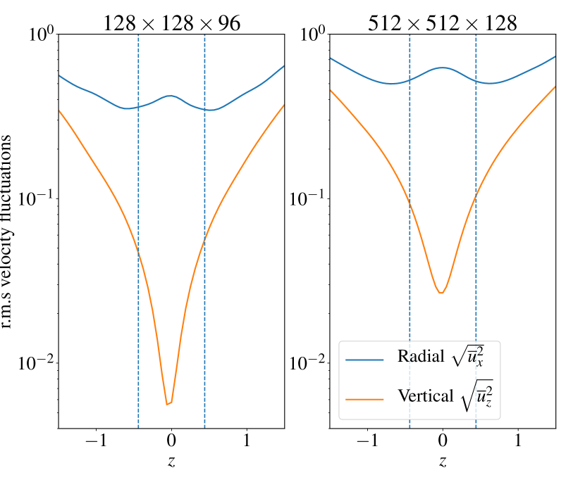
Figure 1: Mean vertical profiles of the gravito-turbulent r.m.s velocities, normalized by $c_{s_{0}}$. The quantities are averaged over time and horizontal plane, with resolution $512\times 512\times 128$ (left) and $128\times 128\times 96$ (right). The time-average is done for $40\,\Omega^{-1}$ for the high resolution run and $100\,\Omega^{-1}$ for the low resolution run. The dashed vertical lines delimit the self-gravitating disc scale-height $H_{g}\simeq 0.44H$.

3.2 Initialization of the dust and settling time

In order to simulate the dust motions unproblematically, we start with the gravito-turbulent state presented above, and introduce grains with initial distribution at $t=0$

$$\rho_{d}(t=0)=\rho_{0}\exp\left(-\dfrac{z^{2}}{2H_{d_{0}}^{2}}\right),$$ (22)

with $H_{d_{0}}=0.5\,H$ and $\rho_{0}$ a constant evaluated so that the ratio of surface densities $\Sigma_{d}/\Sigma$ is $0.0035$ for a single species (or size). The dust velocity is initially unperturbed Keplerian motion. We first conducted simulations at low and intermediate resolution ($N_{X}=N_{Y}\leq 256$), for which we integrate simultaneously the motion of five different grain sizes with Stokes numbers in the midplane 0.16, 0.06, 0.016, 0.006 and 0.0016. We then computed two distinct high resolution ($N_{X}=N_{Y}=512$) simulations, initialized from the same gravito-turbulent state, the first one containing particles with Stokes numbers 0.016 and 0.006, the other containing particles with $\text{St}=0.16$ and $0.06$. Also, for simplicity, the dust mass distribution is initially independent of the particle size, which is not the case in real protoplanetary discs. However we checked that the dust back reaction onto the gas has no important impact on the simulation outcome (see Appendix B). The initial mass distribution is then irrelevant for the dust dynamics in our problem and one can re-normalize the dust density by any given value.

Note that for a given size, the dust-to-gas ratio is not necessarily realistic, though the total dust surface density is $0.0175$ the gas surface density, which is not unreasonable. .

Once the dust is initialized, its time and horizontally-averaged density profiles converge toward a steady state after a characteristic period of time dependant on the Stokes number. Fig. 2 (top and center panels) shows the time evolution of the averaged dust density profile (in $x$ and $y$) for $\text{St}=0.006$ and $\text{St}=0.06$, computed from the high resolution runs. Initially, large grains ($\text{St}=0.06$) fall towards the mid-plane very rapidly, within a time proportional to $\Omega^{-1}/\text{St}\sim 15\,\Omega^{-1}$ (Dullemond & Dominik, 2004). Afterwards, turbulent diffusion and mixing emerge and ultimately balance the gravitational settling. The mean vertical profile of the smaller grains ($\text{St}=0.006$) does not seem to evolve significantly during the simulation because the dust layer is already close to equilibrium initially. However, as the space-time diagram makes clear, on short times the vertical profiles are quite dynamic and, in the case of small dust especially, consist of quasi-periodic vertical compressions and rarefactions, clearly associated with the spiral wave dynamics.

Note that the high resolution simulations are run for a relatively short time ($\lesssim 100\,\Omega^{-1}$) due to the large computing resources they demand. Nevertheless, this time remains longer or comparable to the settling time for most of the Stokes numbers probed. Lower resolution simulations are run for $\sim 150\,\Omega^{-1}$ and we checked that no significant variation of the dust dynamics occurs during this time.

3.3 Dust settling and vertical dynamics

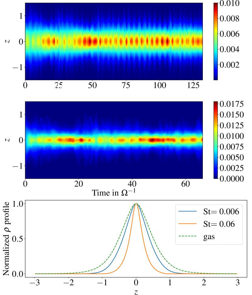
Figure 2: Top and centre panels: space-time diagram ($z$,$t$) showing the dust density distribution, averaged in $x$ and $y$, for $\text{St}=0.006$ and $\text{St}=0.06$ respectively. Bottom panel: dust density profiles averaged in time and normalized to the midplane density for $\text{St}=0.006$ and $\text{St}=0.06$. As a comparison, the green dashed curve describes the gas density profile.

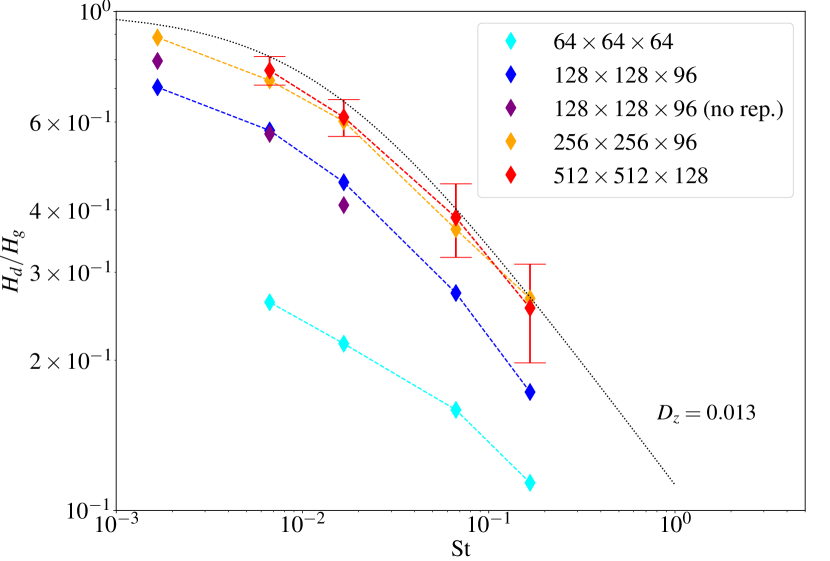
Figure 3: Mean ratio of dust to gas heightscale $H_{d}/H_{g}$ as a function of the Stokes number for different resolution, measured from numerical simulations, with the definition given by Eq. 23. In the high resolution runs we add error bars whose width corresponds to the standard deviation from the time-averaged $H_{d}/H_{g}$. The purple diamonds account for a simulation without replenishment of the dust. The black dotted line is the theoretical prediction from the simple advection-diffusion model described in Section 3.3.2 using a diffusion coefficient $D_{z}=0.013$.

3.3.1 Vertical density profiles and scaleheights

We characterize the long-term dust vertical equilibrium and estimate its typical scale height as a function of the Stokes number. Fig. 2 (bottom panel) shows the mean vertical density profiles, averaged in time (during $130\,\Omega^{-1}$ for $\text{St}=0.006$ and $60\,\Omega^{-1}$ for $\text{St}=0.06$) and obtained in the high resolution runs $(512\times 512\times 128)$. For comparison we superimpose the gas vertical density profile (dashed green line); though not strictly a gaussian, this curve can be fitted rather well with one, with width $H_{g}\simeq 0.44H$.

The dust density profiles can also be approximated by gaussians but with a width smaller than $H_{g}$. We define the dust scaleheight $H_{d}\,(\text{St})$ as the altitude $z$ such that

$$\rho_{d}(z=H_{d})=\rho_{d}(z=0)\,e^{-\frac{1}{2}}\simeq 0.6\,\rho_{d0}.$$ (23)

For each species, we measure this scaleheight and display the time-averaged dust to gas ratio $H_{d}/H_{g}$ in Fig. 3 for various resolutions.

First we see that, independently of resolution, the size of the dust layer increases with decreasing Stokes number. This is to be expected, because small dust particles are less sensitive to gravitational settling and will tend to follow the turbulent gas motion. At larger St, the ratio $H_{d}/H_{g}$ depends on St^-1/2, a result that has been obtained in other simulations coupling dust and turbulent gas (Fromang & Papaloizou, 2006; Okuzumi & Hirose, 2011; Zhu et al., 2015; Yang et al., 2018; Riols & Lesur, 2018). This dependence can be understood, in a rather crude way, within the framework of a simple diffusion theory (Morfill, 1985; Dubrulle et al., 1995, see Section 3.3.2), where the vertical equilibrium is set by the balance between the gravitational settling and turbulent diffusion.

Second, the absolute values of $H_{d}/H_{g}$ increases with the grid resolution. The reason of this dependence may be attributed to the difficulty in simulating the parametric instability, which excites small-scale modes that may enhance diffusion of dust particles. Lower resolution runs do not adequately capture these small-scale modes and hence the diffusion they bring to bear on the dust. Note, however, that convergence does seem to be achieved for a resolution greater than 13 points per $H$ (the case with 13 or 26 points in the horizontal directions showing no major difference).

Third, the size of the dust layer is large for mm to cm particles ($\text{St}\simeq 0.0016$ and $0.016$), larger than $0.85H_{g}$ and $0.6H_{g}$, respectively. This is very similar to what magnetorotational turbulence with a zero-net vertical field can achieve (Fromang & Papaloizou, 2006). These layer thicknesses are interesting since they can be directly measured in cases where the disc is observed edge-on. Indeed, the spatial resolution of instruments like ALMA is sufficient to resolve vertical scales less than $H$ at distances of a few tens of AU (see discussion in Section 4).

Finally, as mentioned already in Section 3.2, Fig .2 indicates that the dust midplane density varies quasi-periodically (with period of a few $\Omega^{-1}$). Concurrently, the dust layer undergoes vertical compression and expansion, which are clearly correlated with the variations of the gas midplane density. Inevitably these oscillations lead to variations in the dust scale height. We thus quantify, for the high resolution runs, the typical deviations of $H_{d}$ (denoted $\delta H_{d}$) and the ratio $H_{d}/H_{g}$ (denoted $\delta H_{d}^{*}$) from their temporal averages. We find that $\delta H_{d}\simeq 0.19,0.16,0.15$ and $0.13\,H_{d}$ respectively for $\text{St}=0.16,0.06,0.016$ and 0.006. In the same order, we find $\delta H_{d}^{*}=0.17,0.12,0.1$ and $0.07\,(H_{d}/H_{g})$. The last values are used to calculate the error bars in Fig. 3. Thus the deviations (or oscillations) remain relatively small compared to the mean values and will be probably undetectable by current instruments measuring the dust scaleheight.

3.3.2 Settling model and diffusion coefficients

We next apply a simple diffusion model (Dubrulle et al., 1995) to explain the equilibrium dust scaleheights measured in the previous section. The model has its limitations; in particular, it assumes that turbulent eddies sizes are less than $H$, whereas the GI vertical rolls occur on scale similar or larger than $H$. Nevertheless, assuming that the theory is marginally applicable, we find (see Appendix A) that the dust to gas scaleheight ratio is

$$\dfrac{H_{d}}{H_{g}}=\left(1+\dfrac{\text{St}\,\Omega f_{c}(s+1)\,H_{g}^{2}}{D_{z}}\right)^{-1/2}.$$ (24)

with $f_{c}\approx 1.3$ a coefficient related to the compressibility of the flow, $s\simeq 2.77$ a coefficient related to the settling due to self-gravity and $D_{z}\simeq\langle\overline{v_{z}^{2}}\rangle$ $\tau_{\text{corr}}$ a constant and uniform diffusion coefficient encapsulating turbulent transport.

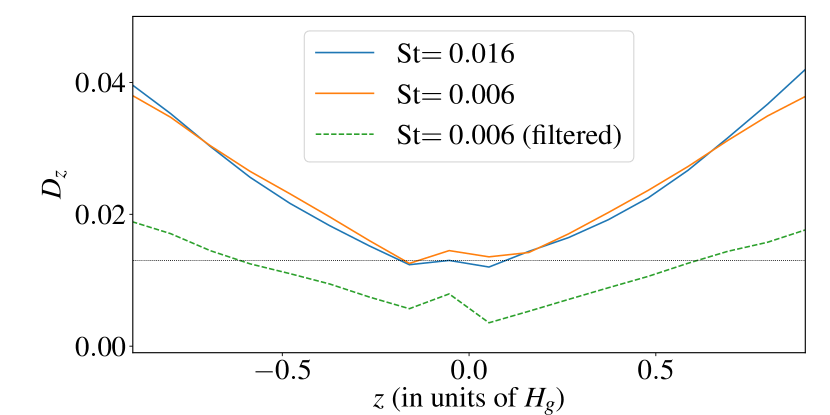
Figure 4: Vertical diffusion coefficients measured in the high resolutions simulations with $N_{X}=N_{Y}=512$. The blue and orange curve are respectively computed for $\text{St}=0.016$ and $\text{St}=0.006$. The green curve is the diffusion coefficient computed by filtering out all the modes $k_{y}>2\pi/L_{y}$ in the calculation of the averaged product $\langle\overline{\delta\rho_{d}\,\delta v_{z_{d}}}\rangle$. This gives an estimate of the diffusion produced by large scale spiral waves only. Note that the small asymmetry about the midplane is potentially due to the fact that the averaging procedure is done over a rather short time ($\sim 100\,\Omega^{-1}$).

We could, of course, apply Eq. (24) to Fig. 3 and find the $D_{z}$ predicted by the theory in each case. Instead, we calculate $D_{z}$ directly from the simulations and subsequently check how well the diffusion theory does in reproducing Fig. 3. We compute the vertical diffusion coefficient from the high resolution simulation data, by averaging in time over $100\,\Omega^{-1}$, the quantity

$$D_{z}=-\dfrac{\langle\overline{\delta\rho_{d}\,\delta v_{z_{d}}}\rangle}{\left\langle\overline{\rho}\dfrac{\partial}{\partial z}\left(\dfrac{\overline{\rho_{d}}}{\overline{\rho}}\right)\right\rangle},$$ (25)

(see Appendix A). Figure 4 shows $D_{z}$ calculated this way for two different Stokes numbers $\text{St}=0.016$ and $\text{St}=0.006$, as a function of $z$. In the midplane we find $D_{z}\simeq 0.013$ roughly for both Stokes numbers, but note that $D_{z}$ increases with altitude $z$, following the r.m.s vertical velocity in Fig. 1. Despite this increase, the hypothesis of constant $D_{z}$ does hold for $z\ll H_{g}$. If next we insert this constant numerical value in place of the diffusion coefficient in Eq. 24, we obtain a ratio $H_{d}/H_{g}$ that reproduces that measured in the high resolution simulation (see dotted black line in Fig. 3). We hence conclude that, to a first approximation, the several turbulent gas flow features acting on the dust work together diffusively, at least on long times. (On short scales, of course, the situation is more interesting and dynamic, as the top two panels of Fig. 2 indicate.)

3.3.3 The relative contributions of vertical rolls and small-scale turbulence to diffusion

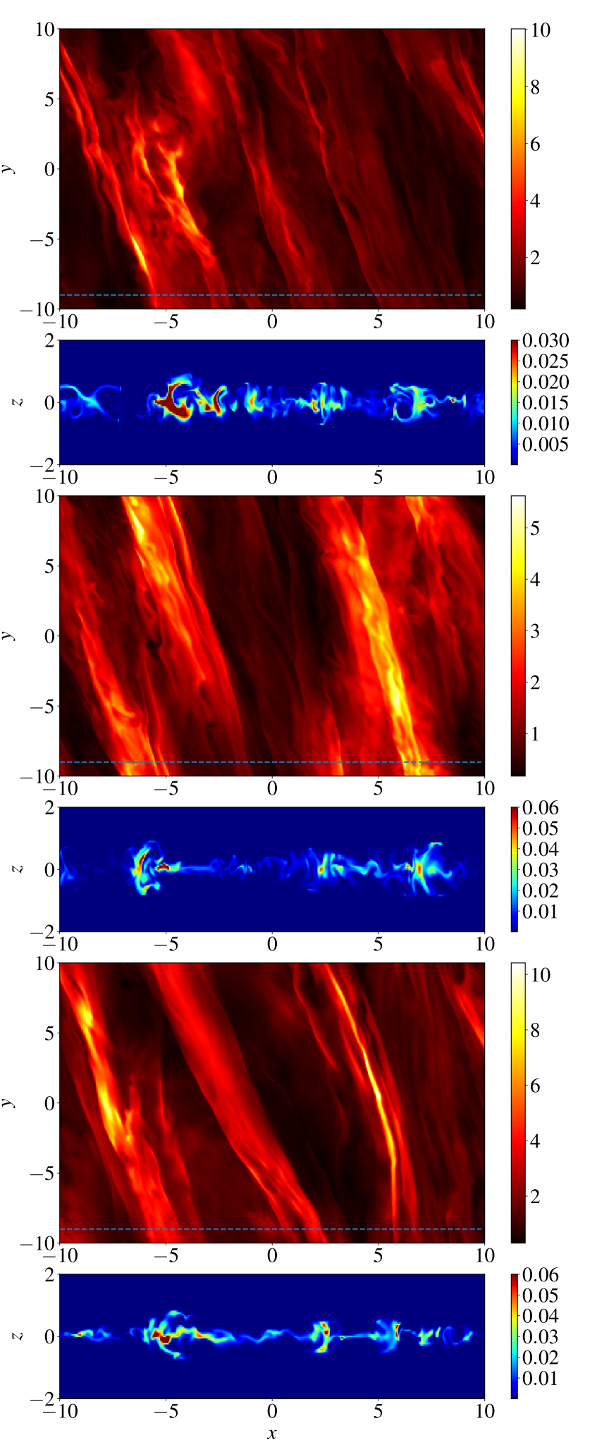
Figure 5: Snapshots of the gas density in the horizontal plane and the dust density in the poloidal plane for $\text{St}=0.06$ and for three different times (from top to bottom : $27\,\Omega^{-1}$, $31\Omega^{-1}$ and $51\,\Omega^{-1}$). The dashed lines in the former denote the location of the poloidal planes.

In the previous subsection we demonstrated that the gravitoturbulence can effectively halt the settling of dust grains. Now we determine what features of the flow are responsible for the vertical diffusion of the particles. In particular, which is more important: small-scale inertial wave turbulence (difficult to simulate because of steep resolution requirements), or large-scale vertical rolls (somewhat more easy to simulate, especially in global set-ups).

We begin by concentrating on the large-scale vertical circulation. As shown by Riols & Latter (2018b), in stratified atmospheres with a mean entropy gradient, these motions are quite generally triggered by baroclinic effects and are composed of a pair of counter-rotating rolls of size $\simeq H_{g}$, travelling in the horizontal direction with the wave. In severe spiral shocks, vertical flows arise also from hydraulic jumps (Boley and Durisen 2006).

In Fig. 5, we show the gas distribution in the horizontal plane and the corresponding dust distribution in a poloidal plane $(y=-9H)$ for $\text{St}=0.06$ at 3 different times. At the location of each spiral wave, the dust distribution forms vertical arcs that locally reach $z\simeq H$. These arcs are clearly the result of dust lifted up by the large-scale rolls. Note that these arcs are not necessarily symmetric with respect to the wave front and are stretched in a privileged direction. Clearly we see a dynamic transport of dust vertically, but it is not guaranteed that, cumulatively, these arcs lead to an appreciable average vertical diffusion of dust (and thus impact on the ratio $H_{d}/H_{g}$). Indeed the inter-arms spirals regions are highly sedimented at the same time these arcs are active.

To make further progress and to develop a more quantitative approach, we remove the contribution of axisymmetric modes and non-axisymmetric modes with $k_{y}>2\pi/L_{y}$ in the calculation of the vertical diffusion coefficient $D_{z}$. This is equivalent to filtering out the small-scale inertial wave turbulence and keeping only the large-scale spiral vertical rolls (with $k_{y}=2\pi/L_{y}$) in the product $\langle\overline{\delta\rho_{d}\,\delta v_{z_{d}}}\rangle$. The related diffusion coefficient $D_{z_{\text{filt}}}$ is shown in dashed green in Fig. 4. We see that the filtered quantity contributes 30 % of the diffusion coefficient in the midplane ($D_{z_{\text{filt}}}\simeq 0.0035$) and rises to 50 % in the corona. Therefore, both the spiral vertical motions and the small-scale inertial waves contribute to the dust diffusion.

In fact, this result may have been expected from Fig. 3, which shows the dependence of $H_{d}/H_{g}$ on resolution. For the lowest resolution $(N_{X}=N_{Y}=64)$, the small-scale turbulence is not properly resolved and its impact in the dynamics diminished, as a consequence; thus the vertical diffusion is accomplished primarily by the vertical rolls, and indeed we see immediately that the dust scale height drops significantly and is well-approximated by a theory using the filtered diffusion coefficient $D_{z_{\text{filt}}}$. At better resolution the small-scale turbulence is better described, vertical diffusion increases as a result, and the dust thickness increases.

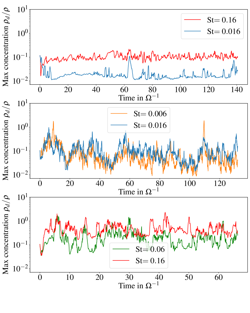
Figure 6: Maximum dust concentration in the box for different Stokes numbers. These are computed for resolutions $128\times 128\times 96$ (top panels) and $512\times 512\times 128$ (middle and lower panels)

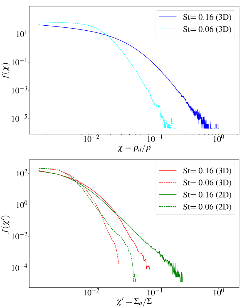
Figure 7: Probability distribution functions $f$ for concentration events. The top panel shows $f(\chi)$ computed from 3D simulations, where $\chi=\rho_{d}/\rho$. The bottom panel shows $f(\chi^{\prime})$ associated with 2D simulations (in green) and 3D simulations (in red) where $\chi^{\prime}=\Sigma_{d}/\Sigma$. The dotted lines are for $\text{St}=0.06$ and the solid lines are for $\text{St}=0.16$.

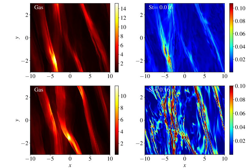
Figure 8: Left panels: snapshots of gas pressure in the midplane at two different times. The top panels are taken at $t=48\Omega^{-1}$ while bottom panels are taken at $t=50\Omega^{-1}$ when the dust to gas ratio reaches a local maximum (we remind the reader that top and bottom are different simulations with different grain size, but with the same initial conditions for the gas) . Right panels correspond to the dust density in the midplane for $\text{St}=0.016$ (top) and $\text{St}=0.16$ (bottom).

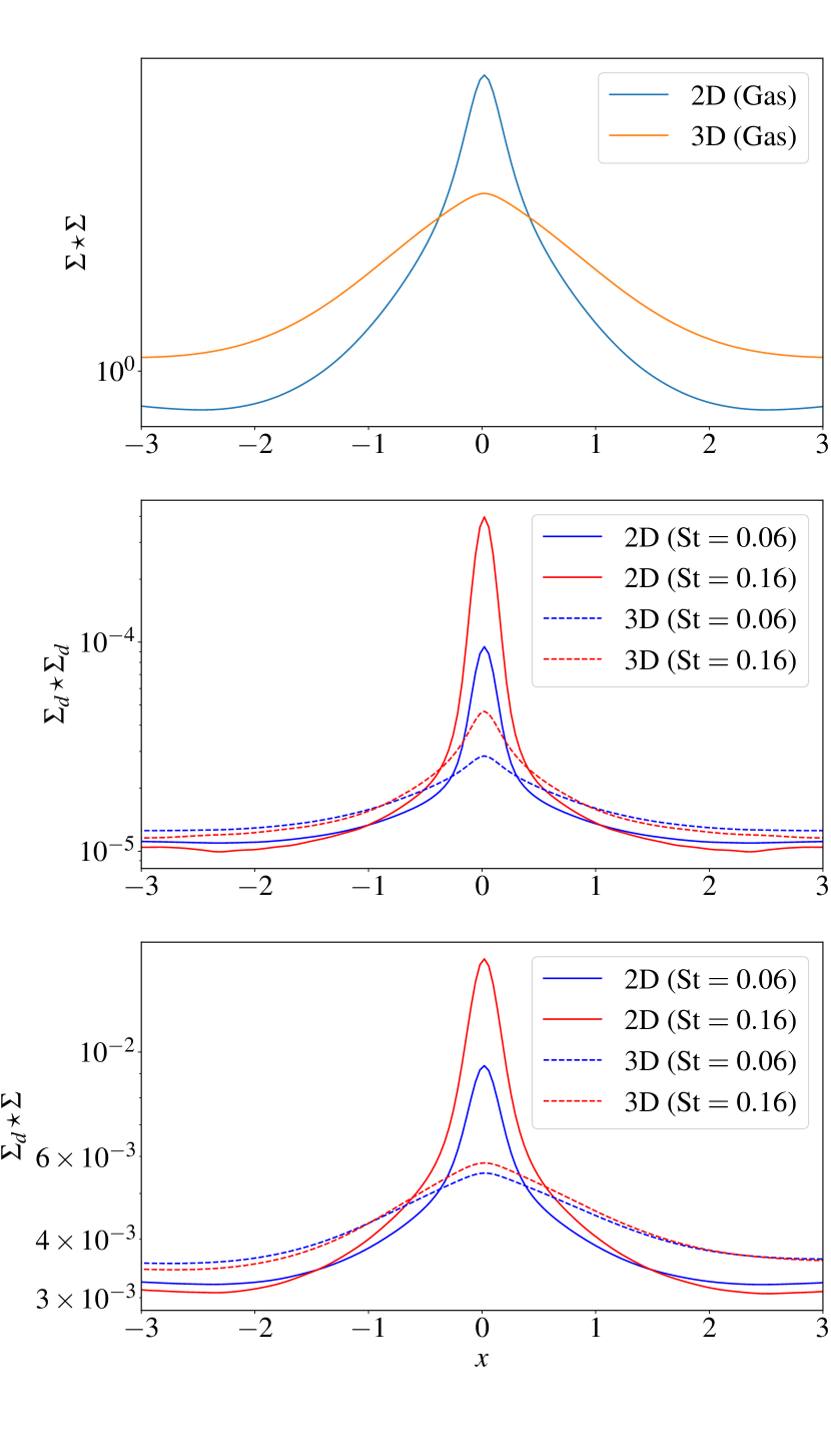
Figure 9: Top and centre panels are, respectively, the autocorrelation functions of the gas and the dust surface density in the radial direction. Bottom panel shows the cross-correlation between gas and dust surface density in the radial direction. Each correlation function is averaged in time.

3.4 Dynamics in the horizontal plane

3.4.1 Concentration events

In this section we analyse the statistics of concentration events, especially those that lead to high dust to gas ratios $\rho_{d}/\rho\gtrsim 1$. In dust rich regions the system might trigger the streaming instability or even the gravitational collapse of the dust, which may be crucial stages in the planet formation process (See Section 1).

Before we present this subsection’s results we must emphasise that they are resolution dependent: specifically, the better the resolution the more likely the dust is to be concentrated. This dependence probably issues from two causes: (a) some of the properties of our simulated small-scale inertial wave turbulence are not converged with respect to resolution, because the parametric instability can inject energy into extremely short scales, shorter than our grid lengths, and (b) the violation of the pressureless fluid approximation for the dust in high resolution runs, because the stopping time may become longer than the turbulent turn-over time on the grid. Certainly, the latter effect will artificially enhance concentration events, and thus our high resolution results may best be understood as providing upper bounds on concentration. Perhaps more robust are the relative trends observed and the differences between 2D and 3D simulations.

First, we show in Fig. 6 the time-evolution of the maximum concentration $\rho_{d}/\rho$ in the box. This concentration, on average, increases with Stokes number, which is expected from physical arguments. Small grains mostly follow the gas motion, whereas particles with Stokes number $0.16$ can drift more easily toward pressure maxima. Fig. 6 shows that in the high resolution runs, and for $\text{St}=0.16$, the concentration of dust rarely exceeds 1 during the first tens of orbits. Obviously such events are even less frequent for small particles but can still occur (for example at $t=10$ and $t=110\,\Omega^{-1}$ for $\text{St}=0.006$). However all these events are short and never last more than an orbit. Note that in our low resolution simulation, significant concentration events do not occur (see discussion above).

To further investigate the occurrence of particle concentration, we show in Fig. 7 the probability distribution function $f(\chi)$ for concentration events, computed for two different Stokes numbers in the midplane region ($|z|\leq 0.4H$). If we set $\chi=\rho_{d}/\rho$, the function $f(\chi)$ is obtained by counting the number of cells within the midplane that contain a given concentration $\chi$, at any given time. The function is averaged in time and then normalized so that its integral over the domain of $\chi$ considered is 1. We find again that the largest Stokes number $\text{St}=0.16$, which corresponds to a grain of decimetre size, favours higher dust concentration. The function has a small tail at $\chi\lesssim 1$, but the probability of $\chi=\rho_{d}/\rho\gtrsim 1$ is almost zero and concentration events are very rare.

In the lower panel of Fig. 7, we compare this result with 2D planar simulations possessing the same Stokes numbers, cooling time, and initial surface densities. Note that the 2D simulations are performed without a smoothed potential in the vertical direction, and thus solve

$$\mathbf{\nabla}^{2}\Phi_{s}=4\pi G\rho(x,y)\delta(z).$$ (26)

with $\delta$ the Dirac function. To make the comparison possible, we compute the probability distribution function for the ratio of surface densities $\chi^{\prime}=\Sigma_{d}/\Sigma$. The result is that the tail of the distribution function in 2D simulations extends to larger $\chi^{\prime}$, and hence stronger concentration events are more likely. One hence concludes that the inclusion of additional 3D flows works against the formation of dense columns of dust, probably via a combination of vertical redistribution of dust by the vertical rolls and small-scale inertial wave turbulence.

3.4.2 Grain distribution within spiral waves

Although the concentration of sub-decimetre dust grains seems to barely reach 1, it is of interest to determine how the dust is distributed horizontally. We find that grains are mostly concentrated into the pressure maxima associated with spiral waves, in agreement with previous work (Gibbons et al., 2012, 2015; Shi et al., 2016). To illustrate this result, we show in Fig. 8 two snapshots of the gas pressure and dust density taken from the high resolution simulations. The upper right panel corresponds to $\text{St}=0.016$ at a random time, while the lower right panel corresponds to $\text{St}=0.16$ at $t=50\,\Omega^{-1}$ when the concentration reaches a local maximum $\rho_{d}/\rho\simeq 1$. Clearly small particles are well coupled to the gas and therefore display a similar density structure. Particles possessing the longer stopping time $\text{St}=0.16$ concentrate in thin filaments, located within the spiral waves, and exhibiting densities two or three order of magnitude greater than the background dust density.

To be more quantitative, we analyse the typical length-scales of the gaseous and dust structures in the radial direction. For that purpose, we introduce the two auto-correlation functions $\Sigma\star\Sigma(x)$ and $\Sigma_{d}\star\Sigma_{d}(x)$ (see definitions in Section 2.5), averaged in time during the course of the simulation. The typical width of these functions (which is taken as $2x$ with $x$ corresponds to the radius of half their peak amplitude) account respectively for the size of the gas spiral arms and the dust structures in the radial direction.

Figure 9 (top) shows $\Sigma\star\Sigma$ for different 2D and 3D runs. For a similar box size $L_{x}=20H$, the spiral arms obtained in 2D are two times thinner than those obtained in 3D. For reference, we denote by $\lambda_{2d}$ and $\lambda_{3d}\simeq 2H$ these different scales associated with the gas spiral structures. Figure 9 (center panel) shows the auto-correlation functions of the dust $\Sigma_{d}\star\Sigma_{d}$ for 2D and 3D runs and for Stokes numbers St $=0.06$ and St $=0.16$. Clearly 2D dust structures are much thinner than those in 3D. The dust filaments in 2D have lengthscale between $0.18$ and $0.25\lambda_{2d}$ while in 3D the structures are much wider with typical size between $0.4$ and $0.8\lambda_{3d}$ (comparable to the gas spiral arms). We checked also that the dust is concentrated into thinner structures when the Stokes number increases, which is expected.

Finally, to understand the distribution of dust relative to the gas, we introduce the cross-correlation function $\Sigma_{d}\star\Sigma$ displayed in the bottom panel of Fig. 9. Clearly, for all cases, the cross-correlation has a maximum at $x=0$ suggesting that the dust is trapped, on average, into the density maxima of the gas corresponding to spiral waves. More interestingly, the correlation is higher in 2D than in 3D and the typical correlation length is smaller in the 2D case ($\simeq 0.5\lambda_{2d}$ in 2D versus $\simeq 2\lambda_{3d}$ in 3D). Physically this means that in 3D, diffusion of dust is enhanced and counteracts the process of grain accumulation inside spiral waves.

4 Discussion and Conclusions

In this paper, we simulated dust dynamics in gravitoturbulent accretion discs. Our special focus was on the action of secondary 3D flows associated with the spiral waves (vertical rolls and inertial wave turbulence), and thus we employed high resolution vertically stratified shearing boxes, using the code PLUTO.

First, we showed that both small-scale GI motions and large-scale vertical rolls associated with spiral waves act to diffuse the grains in the vertical direction. We calculated the steady-state dust scaleheights as a function of Stokes number, and showed that a simple diffusion model (like that employed by Dubrulle et al., 1995) is sufficient to explain the scaleheights measured in simulations. Note that the Schmidt number, the ratio of turbulent viscosity to particle diffusion coefficient

$$\text{S}_{c}=\nu_{t}/D_{z}=\alpha H^{2}\Omega/D_{z}=H^{2}/(q(\gamma-1)\tau_{c}D_{z}),$$ (27)

(assuming Eq. 21 for $\alpha$) is of order 4, twice that measured in the radial direction in 2D simulations (Shi et al., 2016). Overall, we find that GI significantly impedes the settling of intermediate size grains: quasi-steady dust scale-heights are roughly half or more the accompanying gas scale height. This is perhaps the most interesting, and most robust, result in this paper.

Second, we studied the dynamics in the horizontal direction and found that concentration of grains into pressure maxima (i.e spiral waves) is less pronounced in 3D than in 2D, although small-scale filamentary structures embedded in the spiral waves still occur. The ratio $\rho_{d}/\rho$ never exceeds 1 and transient concentration events possess timescales that barely reach an orbit for grains below the decimetre size. We stress, however, that these results suffer from resolution non-convergence, issuing either from our fluid model for the dust or the difficulty in simulating the small-scale turbulence.

Lastly, we showed that the typical horizontal lengthscale of dust spiral structure in 3D is longer than that of gas spiral arms for $\text{S}t\lesssim 0.2$, and in particular significantly longer than in comparable 2D runs. This suggests that additional 3D flows act to diffuse the grain in the radial direction and prevent its concentration into the pressure maxima. In other words, the secondary vertical rolls and small-scale inertial turbulence help ‘blur’ the signature of the gas’s spiral waves in the horizontal dust distribution.

Our results have several implications for young and massive protoplanetary discs and their observations. First, they invite us to reassess the conclusions of previous 2D studies on the formation of planetesimals by GI (Gibbons et al., 2012, 2015; Shi et al., 2016). Three dimensional flows disfavour the concentration of grains, via their retardation of vertical settling and via radial diffusion. Consequently, these flows indirectly inhibit the streaming instability acting on centimetre to decimetre sizes (Youdin & Goodman, 2005) and the direct gravitational collapse of such grains.

Second, and on the other hand, the inefficient sedimentation of sub-millimetre particles could help us infer the existence of gravito-turbulence in the outer radii of protoplanetary discs. At these radii, non-ideal effects, in particular ambipolar diffusion, is believed to quench the magneto-rotational instability (Fleming et al., 2000; Sano & Stone, 2002; Wardle & Salmeron, 2012; Bai & Stone, 2013; Lesur et al., 2014; Bai, 2015) and prevent any form of turbulence originating from MHD effects. Thus a low level of settling measured in observed discs is likely to be induced by hydrodynamic turbulence such as GI (or the VSI if sufficiently strong, see Stoll & Kley, 2016; Lin, 2019) In the coming years, the radio-interferometer ALMA will be able to study a large sample of ‘edge-on’ discs and the sufficient resolution to measure the dust scaleheight in these systems. The comparison between these scaleheight and those simulated will be directly relevant to assess the presence of GI in these discs.

Finally, the 3D flows accompanying spiral arms in GI could have a direct impact on the scattered infra-red luminosity measured from observations. We have shown that small dust particles (with stopping times much less than $\Omega^{-1}$) are lofted efficiently above the spiral patterns at the disc surface, and also mixed in the upper layers by small-scale turbulence. As a result the surface emission properties of the disk will be altered.

Appendix A Settling model

We use here the simple diffusion theory of Dubrulle et al. (1995) to estimate the dust scaleheight in gravito-turbulence. In this model, it is assumed there is some ‘small-scale’ turbulence, with a characteristic horizontal lengthscale, a characteristic vertical lengthscale $\ll H$, and a timescale of order an orbit. In addition, there is a large-scale mean component that varies on long times, much longer than an orbit, and exhibits variations only in $z$, of an order the disk scaleheight, $H$.

We introduce fast variables $\mathbf{x}\textquoteright$ and $t\textquoteright$, which vary on the turbulent scales, and slow variables $z$ and $t$, which vary on the long mean scales (see Latter & Balbus, 2012). Next all quantities are decomposed into mean and fluctuating parts

$$\rho_{d}=\overline{\rho_{d}}+\delta\rho_{d};\quad\mathbf{v}=\overline{\mathbf{v}}+\delta\mathbf{v};\quad\mathbf{v_{d}}=\overline{\mathbf{v_{d}}}+\delta\mathbf{v_{d}},$$ (28)

with the mean parts depending only on the slow variables and the fluctuating parts depending on both slow and fast variables. To formally distinguish the two components we introduce the average $\overline{f}=\int fd\mathbf{x}\textquoteright dt\textquoteright$, which integrates over sufficient turbulent length and time scales so that $\overline{f}$ only depends on the slow variables, where $f$ is any field and $\delta f$ is the fluctuating component of that field.

The averaged mass conservation equation (7) can be written as:

$$\dfrac{\partial\overline{\rho_{d}}}{\partial t}+\dfrac{\partial}{\partial z}\left(\overline{\rho_{d}}\,\overline{v_{z}}+\overline{\delta\rho_{d}\,\delta v_{z_{d}}}+\overline{\rho_{d}}\,\overline{\Delta v_{z}}\right)=0,$$ (29)

where $\mathbf{\Delta v}=\mathbf{v}_{d}-\mathbf{v}$ is the drift velocity between dust and gas. The first term in the $z$-derivative corresponds to the advection-stretching of dust by the mean vertical gas flow (wind), which appears to be negligible in our numerical simulations. The second term is the correlation of turbulent fluctuations which is approximated by a diffusion operator in Dubrulle’s theory. The third term accounts for the mean vertical drift of dust due to gravitational settling (including the self-gravity of the disc). Using classical assumptions, detailed in Section 5.1.2 and Appendix B of Riols & Lesur (2018), in particular the terminal velocity approximation, it is possible to recast Eq. (29) in the useful form of an advection-diffusion equation:

$$\dfrac{\partial\overline{\rho_{d}}}{\partial t}=\dfrac{\partial}{\partial z}\left[\left(z\Omega^{2}+\dfrac{d\Phi_{s}}{dz}\right)\,\overline{\tau_{s}}\,\overline{\rho_{d}}\right)+\dfrac{\partial}{\partial z}\left[D_{z}\,\overline{\rho}\dfrac{\partial}{\partial z}\left(\dfrac{\overline{\rho_{d}}}{\overline{\rho}}\right)\right],$$ (30)

where $D_{z}\simeq\langle\overline{v_{z}^{2}}\rangle$ $\tau_{\text{corr}}>0$ is the diffusion coefficient, with $\tau_{\text{corr}}$ the correlation time of the turbulent eddies. Note that the horizontally averaged Stokes number ${\overline{\tau_{s}}=\text{St}\Omega^{-1}\overline{\rho_{0}/\rho}}$ is slightly different from ${\text{St}\Omega^{-1}\rho_{0}/\overline{\rho}}$. Due to gas density fluctuations associated with GI, there is a factor $f_{c}\simeq 1.3$ difference between the two quantities. This factor is obtained from simulations by averaging in $x$ and $y$ the inverse of the gas density. We finally assume that the gas density can be modelled by a Gaussian ${\rho=\rho_{0}\exp{(-\frac{z^{2}}{2H_{g}^{2}})}}$ with midplane $\rho_{0}=1.57$ and $H_{g}=0.44H$. This hypothesis is not too far from reality for $Q\gtrsim 1$. Under this assumption, we approximate ${d\Phi_{s}}/{dz}\simeq sz\Omega^{2}$ with $s=2.77$ in the limit $z\ll H_{g}$.

The equilibrium solution of Eq. (30) is

$$\rho_{d}(z)=\rho_{d_{0}}\exp\left(-\dfrac{z^{2}}{2H_{g}^{2}}\right)\exp\left(-\int\dfrac{\text{St}\,\Omega f_{c}(s+1)\,z\,e^{\frac{z^{2}}{2H_{g}^{2}}}}{D_{z}(z)}dz\right).$$ (31)

For uniform diffusion coefficient $D_{z}$ and $z\ll H_{g}$, this gives:

$$\rho_{d}(z)\simeq\rho_{d_{0}}\exp\left(-\dfrac{z^{2}}{2H_{d}^{2}}\right)$$ (32)

$$\text{with }\quad\dfrac{H_{d}}{H_{g}}=\left(1+\dfrac{\text{St}\,\Omega f_{c}(s+1)\,H_{g}^{2}}{D_{z}}\right)^{-1/2}.$$ (33)

The distribution is Gaussian and the dust scaleheight tends towards unity in the limit of small St. For larger values (but potentially still $<1$), the ratio may exhibit the scaling $\text{St}^{-1/2}$.

Appendix B Simulation without back reaction

We show in this appendix the results of a simulation without the dust back reaction onto the gas. This simulation has been run for $45\Omega^{-1}$ with resolution of 26 points per $H$ in the horizontal direction and contains two species with $\text{St}=0.06$ and $\text{St}=0.16$. We aim to compare this with other simulations including the back reaction (and same setup and Stokes numbers). First we show in Fig. 10 the dust density profile (averaged in $t$, $x$, and $y$). For both Stokes numbers, we find that the profiles are almost indiscernible from each other. This means that the settling process is unaffected by the dust back-reaction.

To go further, we show in Fig. 11 the probability distribution function $f(\chi^{\prime})$ of concentration events (see Section 3.4.1 for details about its calculation), computed for our two different Stokes numbers, in the case with and without back reaction. Again we see only marginal differences between the two cases suggesting that the dust back reaction does not interfere too much with the process of dust concentration and clumping. A slight deviation is however seen at large $\chi^{\prime}=\Sigma_{d}/\Sigma$ for $\text{St}=0.06$ (in the tail of the distribution) but this is expected since the number of events is rare and the statistics not very good at large concentration $\chi^{\prime}$ (given the time of the simulation).

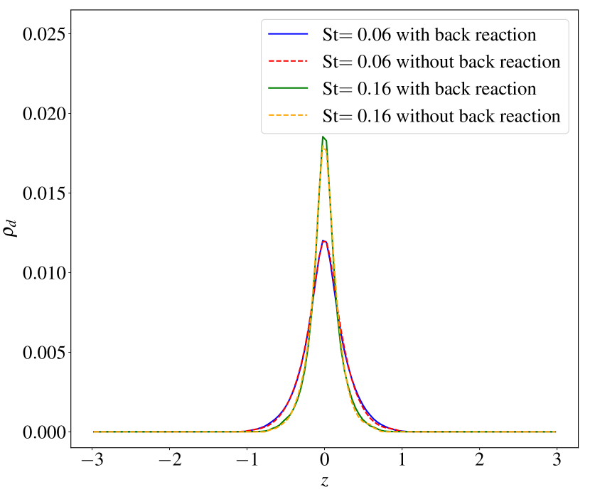
Figure 10: Dust density profiles (averaged in time, $x$ and $y$) for two different Stokes number, with and without back reaction.

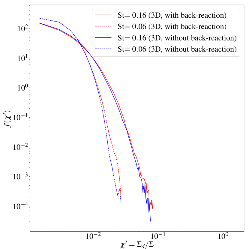
Figure 11: Probability distribution function for concentration events as a function of $\chi^{\prime}=\Sigma_{d}/\Sigma$. The dotted lines are for $\text{St}=0.06$ and the solid lines are for $\text{St}=0.16$. We compare the cases with (red) and without (blue) dust back reaction

References

- ALMA Partnership et al. (2015) ALMA Partnership et al., 2015, ApJl, 808, L3
- Baehr & Klahr (2019) Baehr H., Klahr H., 2019, ApJ, 881, 162
- Bai (2015) Bai X.-N., 2015, ApJ, 798, 84
- Bai & Stone (2010) Bai X.-N., Stone J. M., 2010, ApJ, 722, 1437
- Bai & Stone (2013) Bai X.-N., Stone J. M., 2013, ApJ, 767, 30
- Boley et al. (2005) Boley A. C., Durisen R. H., Pickett M. K., 2005, The Three-Dimensionality of Spiral Shocks: Did Chondrules Catch a Breaking Wave?. p. 839
- Booth & Ilee (2020) Booth A. S., Ilee J. D., 2020, MNRAS, p. L14
- Cuzzi et al. (2008) Cuzzi J. N., Hogan R. C., Shariff K., 2008, ApJ, 687, 1432
- Dong et al. (2015) Dong R., Hall C., Rice K., Chiang E., 2015, ApJ, 812, L32
- Dong et al. (2016) Dong R., Vorobyov E., Pavlyuchenkov Y., Chiang E., Liu H. B., 2016, ApJ, 823, 141
- Dubrulle et al. (1995) Dubrulle B., Morfill G., Sterzik M., 1995, ICARUS, 114, 237
- Duchene et al. (2019) Duchene G., Ménard F., Stapelfeldt K., Villenave M., Flores C., Wolff S., Padgett D., Pinte C., 2019, in American Astronomical Society Meeting Abstracts #233. p. 317.06
- Dullemond & Dominik (2004) Dullemond C. P., Dominik C., 2004, AAp, 421, 1075
- Durisen et al. (2007) Durisen R. H., Boss A. P., Mayer L., Nelson A. F., Quinn T., Rice W. K. M., 2007, Protostars and Planets V, pp 607–622
- Fleming et al. (2000) Fleming T. P., Stone J. M., Hawley J. F., 2000, ApJ, 530, 464
- Fromang & Papaloizou (2006) Fromang S., Papaloizou J., 2006, AAp, 452, 751
- Gammie (2001) Gammie C. F., 2001, ApJ, 553, 174
- Gibbons et al. (2012) Gibbons P. G., Rice W. K. M., Mamatsashvili G. R., 2012, MNRAS, 426, 1444
- Gibbons et al. (2015) Gibbons P. G., Mamatsashvili G. R., Rice W. K. M., 2015, MNRAS, 453, 4232
- Goldreich & Lynden-Bell (1965) Goldreich P., Lynden-Bell D., 1965, MNRAS, 130, 125
- Huang et al. (2018) Huang J., et al., 2018, ApJ, 869, L43
- Latter & Balbus (2012) Latter H. N., Balbus S., 2012, MNRAS, 424, 1977
- Latter & Papaloizou (2017) Latter H. N., Papaloizou J., 2017, MNRAS, 472, 1432
- Lesur et al. (2014) Lesur G., Kunz M. W., Fromang S., 2014, AAp, 566, A56
- Lin (2019) Lin M.-K., 2019, MNRAS, 485, 5221
- Liu et al. (2016) Liu H. B., et al., 2016, Science Advances, 2, e1500875
- Louvet et al. (2018) Louvet F., Dougados C., Cabrit S., Mardones D., Ménard F., Tabone B., Pinte C., Dent W. R. F., 2018, AA, 618, A120
- Manara et al. (2018) Manara C. F., Morbidelli A., Guillot T., 2018, AAp, 618, L3
- Mann et al. (2015) Mann R. K., Andrews S. M., Eisner J. A., Williams J. P., Meyer M. R., Di Francesco J., Carpenter J. M., Johnstone D., 2015, ApJ, 802, 77
- Mignone et al. (2007) Mignone A., Bodo G., Massaglia S., Matsakos T., Tesileanu O., Zanni C., Ferrari A., 2007, ApJs, 170, 228
- Morfill (1985) Morfill G. E., 1985, in Lucas R., Omont A., Stora R., eds, Birth and the Infancy of Stars.
- Najita & Kenyon (2014) Najita J. R., Kenyon S. J., 2014, MNRAS, 445, 3315
- Okuzumi & Hirose (2011) Okuzumi S., Hirose S., 2011, ApJ, 742, 65
- Pérez et al. (2016) Pérez L. M., et al., 2016, Science, 353, 1519
- Picogna et al. (2018) Picogna G., Stoll M. H. R., Kley W., 2018, AAp, 616, A116
- Pinte et al. (2016) Pinte C., Dent W. R. F., Ménard F., Hales A., Hill T., Cortes P., de Gregorio-Monsalvo I., 2016, ApJ, 816, 25
- Rice et al. (2003) Rice W. K. M., Armitage P. J., Bate M. R., Bonnell I. A., 2003, MNRAS, 339, 1025
- Rice et al. (2006) Rice W. K. M., Lodato G., Pringle J. E., Armitage P. J., Bonnell I. A., 2006, MNRAS, 372, L9
- Rice et al. (2011) Rice W. K. M., Armitage P. J., Mamatsashvili G. R., Lodato G., Clarke C. J., 2011, MNRAS, 418, 1356
- Riols & Latter (2018a) Riols A., Latter H., 2018a, MNRAS, 474, 2212
- Riols & Latter (2018b) Riols A., Latter H., 2018b, MNRAS, 476, 5115
- Riols & Lesur (2018) Riols A., Lesur G., 2018, AA, 617, A117
- Riols et al. (2017) Riols A., Latter H., Paardekooper S.-J., 2017, MNRAS, 471, 317
- Sano & Stone (2002) Sano T., Stone J. M., 2002, ApJ, 577, 534
- Sheehan & Eisner (2018) Sheehan P. D., Eisner J. A., 2018, ApJ, 857, 18
- Shi & Chiang (2013) Shi J.-M., Chiang E., 2013, ApJ, 764, 20
- Shi et al. (2016) Shi J.-M., Zhu Z., Stone J. M., Chiang E., 2016, MNRAS, 459, 982
- Simon et al. (2015) Simon J. B., Lesur G., Kunz M. W., Armitage P. J., 2015, MNRAS, 454, 1117
- Stoll & Kley (2016) Stoll M. H. R., Kley W., 2016, AAp, 594, A57
- Tobin et al. (2013) Tobin J. J., et al., 2013, ApJ, 779, 93
- Toomre (1964) Toomre A., 1964, ApJ, 139, 1217
- Wardle & Salmeron (2012) Wardle M., Salmeron R., 2012, MNRAS, 422, 2737
- Weidenschilling (1977) Weidenschilling S. J., 1977, MNRAS, 180, 57
- Yang et al. (2017) Yang C.-C., Johansen A., Carrera D., 2017, AAp, 606, A80
- Yang et al. (2018) Yang C.-C., Mac Low M.-M., Johansen A., 2018, ApJ, 868, 27
- Youdin & Goodman (2005) Youdin A. N., Goodman J., 2005, ApJ, 620, 459
- Zhu et al. (2015) Zhu Z., Stone J. M., Bai X.-N., 2015, ApJ, 801, 81