Discrimination and estimation of incoherent sources under misalignment

Abstract

Spatially resolving two incoherent point sources whose separation is well below the diffraction limit dictated by classical optics has recently been shown possible using techniques that decompose the incoming radiation into orthogonal transverse modes. Such a demultiplexing procedure, however, must be perfectly calibrated to the transverse profile of the incoming light as any misalignment of the modes effectively restores the diffraction limit for small source separations. We study by how much can one mitigate such an effect at the level of measurement which, after being imperfectly demultiplexed due to inevitable misalignment, may still be partially corrected by linearly transforming the relevant dominating transverse modes. We consider two complementary tasks: the estimation of the separation between the two sources and the discrimination between one and two incoherent point sources. We show that, although one cannot fully restore super-resolving powers even when the value of the misalignment is perfectly known its negative impact on the ultimate sensitivity can be significantly reduced. In the case of estimation we analytically determine the exact relation between the minimal resolvable separation as a function of misalignment whereas for discrimination we analytically determine the relation between misalignment and the probability of error, as well as numerically determine how the latter scales in the limit of long interrogation times.

I Introduction

Quantum theory has, over the years, exhibited an innate ability to surpass the limitations in performance set by classical devices in a variety of tasks Gisin and Thew (2007); Smith (2010); Degen et al. (2017); Pirandola et al. (2018) arguably none more so than in the field of statistical inference and decision theory. There the use of distinctive quantum features, such as coherence and entanglement, allows for the existence of ultra-precise measurements Degen et al. (2017) that greatly enhance the performance in a variety of sensing tasks—ghost imaging Lemos et al. (2014) and quantum illumination Lloyd (2008) to name but a few—that are impossible to achieve by even the best classical means.

One such success of the quantum mechanical formalism concerns the spatial resolution of imaging devices. For over a century it was believed that two sources of incoherent light can barely be resolved if “the maximum of one is over the minimum of the other” Rayleigh (1879); any closer than this and conventional classical imaging techniques cannot resolve the two incoherent sources, even if an asymptotically large number of photons are detected. Despite several efforts Acuna and Horowitz (2002); Shahram and Milanfar (2004); Ram et al. (2006); Shahram and Milanfar (2006) this limitation of optical imaging systems—known as the diffraction or Rayleigh limit Rayleigh (1879)—seemed insurmountable until a proper quantum mechanical treatment of the problem revealed that, just like many other classically derived limitations, it too can be overcome Tsang et al. (2016). Rather than imaging directly the incoming radiation it was proven that a simple linear-optical preprocessing of the spatial profile of the electromagnetic field into a predefined set of spatially orthogonal modes, e.g., the Hermite-Gauss modes in case of Gaussian apertures Svelto (1998), followed by photon detection over sufficiently long integration time is capable of resolving two incoherent point sources at arbitrary separation. The reason for this drastic improvement is intuitive: spatially orthogonal modes of light provide information about spatial correlations of the incoming photons, whereas direct imaging does not.

The technique of decomposing, or demultiplexing, the optical field into spatially orthogonal modes followed by photon counting has gained increased attention with rapid theoretical and experimental developments (see Tsang (2020) for a recent review). Its performance has been proven not only in complex estimation tasks, such as resolving multiple sources Tsang (2017, 2019); Zhou and Jiang (2019); Bisketzi et al. (2019); Sidhu and Kok (2017, 2018), sources of unequal brightness Řehaček et al. (2017); Řeháček et al. (2018), sources emitting coherent Tsang and Nair (2019) or non-classical Lupo and Pirandola (2016) light, as well as sources localised arbitrarily in space Prasad and Yu (2019), but also for the closely related problem of discrimination beyond the diffraction limit Lu et al. (2018).

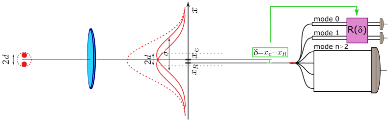
Figure 1: Super-resolving the separation between incoherent sources under the misalignment of the imaging apparatus. Two incoherent point-like sources of light are imaged with an optical system exhibiting a Gaussian point spread function of width $\sigma$ in a way that their separation, $2d$, can be most accurately resolved. For this to be possible beyond the diffraction limit, a spatial mode demultiplexing technique is employed—which ideally allows the incoming light to be decomposed into orthogonal transverse modes, whose photon-occupation is subsequently measured. In this work, we study the ultimate limits on the resolution in the presence of misalignment of the imaging system, $\delta=x_{\mathrm{c}}-x_{R}\ll\sigma$, by applying appropriate linear optical post processing operations $R(\delta)$ is applied on the two dominant modes of the demultiplexing measurement.

Moreover, the robustness to imperfections of the proposed schemes has recently been an object of intensive research Len et al. ; Lupo (2020); Gessner et al. (2020), largely motivated by the challenges imposed by up-to-date experimental demonstrations Paúr et al. (2016); Yang et al. (2016); Tham et al. (2017); Donohue et al. (2018); Parniak et al. (2018); Zhou et al. (2019); Paúr et al. (2018). An important obstacle pointed out in the original paper of Tsang et al. Tsang et al. (2016) is the crucial assumption that the centroid ($x_{\mathrm{c}}$)—the midpoint between the two light sources whose separation, $2d$, is to be resolved—is perfectly aligned ($x_{\mathrm{c}}=x_{R}$) with the detector position ($x_{R}$)—where the spatial transverse modes are demultiplexed. In the presence of any misalignment, $\delta=x_{\mathrm{c}}-x_{R}$ (see Fig. 1), the Fisher information, $F$, that quantifies the ultimate resolution no longer approaches a constant with vanishing separation but rather behaves as $F\sim(d/\delta)^{2}\to 0$ for $d\to 0$ Tsang et al. (2016).

Although the location of the centroid can be estimated via direct imaging, this requires sacrificing an, in principle large amount, of photons in order to do so. A way of leveraging the use of photons between direct imaging and spatial mode demultiplexing, using information of the former to better position the latter, has been recently proposed Grace et al. (2020). Here, in contrast, we take misalignment as experimental fact and investigate the theoretical limits imposed by any misalignment in both the canonical estimation task Tsang et al. (2016); Len et al. ; Lupo (2020); Gessner et al. (2020); Paúr et al. (2016); Yang et al. (2016); Tham et al. (2017); Donohue et al. (2018); Parniak et al. (2018); Zhou et al. (2019); Paúr et al. (2018); Grace et al. (2020) as well as the complementary task of hypothesis testing Krovi et al. (2016); Lu et al. (2018).

Specifically, we ask the following questions; how do estimation precision and the minimal resolvable distance scale as a function of misalignment in the canonical estimation task and, how does the probability of error—both in single observation, as well as asymptotically—depend on misalignment in a typical hypothesis testing task. We keep our treatment as general as possible by considering the use of passive linear optics after the demultiplexing stage (see Fig. 1). We show that even if the value of misalignment $\delta$ is perfectly known such linear optical post processing is not capable of restoring the super-resolution. We demonstrate that optical post-processing of the two most dominants modes, tailored to the misalignment $\delta$, improves estimation precision over the “raw” demultiplexed measurements from $F\propto 1/\delta^{2}$ to $F\propto 1/\delta^{6}$ as $\delta\approx 0$ and the minimal resolvable distance from $\epsilon_{\min}\propto\delta^{\frac{1}{2}}$ to $\epsilon_{\min}\propto\delta^{\frac{3}{2}}$ for both Gaussian and Sinc point-spread functions. Moreover, for single-shot ($n=1$) discrimination the probability of erroneously interpreting a single source for a double one scales as $P_{\textrm{err}}\propto\delta^{6}$ compared to $P_{\textrm{err}}\propto\delta^{2}$ for the misaligned demultiplexed measurements for small $\delta\approx 0$. Furthermore, we also show that linear post-processing also helps in the asymptotic $n\to\infty$ regime, where we observe an enhancement of up to $12\%$ in the exponential decay of the total probability of error.

One may object that if the misalignment is known, then super-resolution can easily be restored simply by adjusting the demultiplexing device to the right position. We stress, however, that in our work this assumption is made in order to explore the theoretical limits on super-resolution allowed by the most general post-processing after an imperfect demultiplexing procedure. From this point of view, our results directly link pertinent quantities, the quantum Fisher information, minimal resolvable distance, and probability of error, to the value of the misalignment. From the practical point of view even if the position of the centroid is perfectly known, fabrication of the demultiplexing measurements, or adjustment of their position via mechanical servo mechanisms entails an inherent uncertainty Morizur et al. (2010) thus not allowing for perfect alignment. In such instances our theoretical analysis offers insight to additional strategies, which may be implemented efficiently by modulating the phase of integrated waveguides Wang et al. (2020); He et al. (2019), that could be used in conjunction to current experimental proposals Grace et al. (2020).

The article is structured as follows. Firstly, we review the necessary mathematical background for both classical and quantum mechanical image resolution in Section II. In Section III we study the effects of misalignment for the problem of estimating the separation between two incoherent point sources, whilst Section IV deals with the effects of misalignment for the problem of discriminating the one versus two sources hypothesis. Section V summarizes our work and discusses possible future directions of investigation.

II Diffraction Limited Optical Imaging

We begin by reviewing the mathematical treatment of optical imaging devices. In Section II.1 we review imaging in classical optics paying particular attention on how the diffraction limit comes about in these set-ups. In Section II.2 we give a formal quantum mechanical description of the point spread function (PSF) of an optical imaging system. We shall restrict our attention particularly to one-dimensional Gaussian and Sinc PSFs but the analysis easily extends to other PSFs and to higher dimensions. We then review a mathematical approximation to the quantum mechanical state of the PSF—the qubit model of Chrostowski et al. Chrostowski et al. (2017). The latter will be used to explore how misalignment of the optical imaging system affects its performance, as well as to propose alternative measurement schemes that compensate for misalignment.

II.1 Classical theory of diffraction limited optical imaging

To image light sources that are far away requires specific lens and aperture systems that allow to process the spatial distribution of the emitters. Assuming the paraxial approximation holds diffraction effects cause variations in radiation intensity at the image plane—the familiar bright and dark fringes in imaging stars, or diffraction gratings. Consequently, the minimum angular distance between two or more emitters that allows their distinction—the angular resolution of the imaging device—is fundamentally limited due to diffraction. Lord Rayleigh was the first to obtain a heuristic rule for the angular resolution of any imaging device Rayleigh (1879): two point sources can barely be resolved so long as the central maximum in intensity of one source lies on top of the first minimum in intensity of the second in the image plane. This rule of thumb is colloquially known as Rayleigh’s curse or diffraction limit in optical imaging.

For the simplest optical imaging device consisting of a single slit of width $D$ the diffraction limit can be deduced by simple geometrical optics, and corresponds to the angular distance, $\phi$, between the central intensity maximum and first minimum which is given by

$$\phi\approx\frac{\lambda}{D}$$ (1)

where $\lambda$ is the wavelength of the incoming radiation, and the approximation sign is due to the paraxial approximation.

More formally, the diffraction limit can be obtained by making use of the Fresnel-Kirchoff formula which describes the amplitude of the disturbance in a given direction, $\phi$, from the optical axis due to the aperture of the imaging system Fowles (1989). For a one-dimensional aperture whose profile is given by $f(y)$, the Fresnel-Kirchoff formula reads

$$\Psi(\phi)=\frac{1}{\sqrt{2\pi}}\int_{-\infty}^{\infty}f(y)e^{\mathrm{i}k\,y\sin\phi}\,\mathrm{d}y,$$ (2)

where $k=2\pi/\lambda$ is the wavenumber. The intensity distribution, also known as the objects point spread function (PSF), at angular separation $\phi$ is given by $\left\lvert\Psi(\phi)\right\rvert^{2}$, and we have implicitly assumed the intensity is normalized $\int\left\lvert\Psi(\phi)\right\rvert^{2}\mathrm{d}\phi=1$. Eq. (2) is the familiar statement that the PSF at the image plane of an image system is the Fourier transform of the systems aperture. The case of the single slit of width $D$ corresponds to $f(y)=\mathrm{rect}\left(-\frac{D}{2},\frac{D}{2}\right)$ and gives rise to the Sinc PSF

$$\Psi(\phi)\propto\mathrm{sinc}\left(\frac{Dk\sin\phi}{2}\right),$$ (3)

here the sinc function is defined as $\mathrm{sinc}(x)=\frac{\sin(x)}{x}$. The first minimum of the sinc function occurs at $\frac{Dk\sin\phi}{2}=\pi$, i.e., $\phi\approx\frac{\lambda}{D}$ which is the result obtained using geometric optics. For a circular aperture $f(y)=\sqrt{D^{2}-4y^{2}}$, where $D$ is the diameter of the aperture, the corresponding PSF reads

$$\Psi(\phi)\propto\frac{J_{1}\left(\frac{Dk}{2}\sin\phi\right)}{\frac{Dk}{2}\sin\phi},$$ (4)

where $J_{1}(z)$ is the Bessel function of the first kind. The first minimum of the latter occurs when $\frac{\pi D\sin\phi}{\lambda}=3.8317$, which sets the angular resolution to $\phi\approx\frac{1.22\lambda}{D}$.

One can, in principle, shape the PSF of an imaging system to any desired function using apodization that suppresses the higher order intensity maxima of the diffraction pattern Debes and Ge (2004). Such techniques can be used to turn the Bessel function PSF of the circular aperture to a Gaussian one. As such techniques do not alter the shape of the aperture, the diffraction limit above still holds.

II.2 Quantum description of two incoherent point sources

Consider two incoherent point sources (e.g., stars or bacteria fluorescing) emitting monochromatic light. We shall assume that the sources are weak, meaning that the average number of photons detected by our imaging device is much smaller than one. Quantum mechanically we may represent the state of the incoming radiation by the density operator Tsang et al. (2016):

$$\sigma^{(i)}\approx(1-\varepsilon)\,|0\rangle\langle 0|+\varepsilon\,\rho^{(i)}+\mathcal{O}(\varepsilon^{2}),$$ (5)

where $\varepsilon\ll 1$, $|0\rangle\langle 0|$ corresponds to the vacuum state, and $\rho^{(i)}\in\mathcal{B}(\mathcal{H}_{1}),\,i\in(1,2)$ is a one-photon state with the superscript index labelling the case where the photon is due to one or two point sources.

As the vacuum offers no information about the nature of the emitting source our only information comes from the single photon events, accumulated over sufficiently long time, at the image plane of our instrument. Assuming the latter to be one-dimensional we define the image plane position eigenkets $|x\rangle=a^{\dagger}(x)|0\rangle$, where $a^{\dagger}(x),\,a(x)$ are the creation and annihilation operators satisfying $[a(x),a^{\dagger}(y)]=\delta(x-y)$ Yuen and Shapiro (1978). The wave function of a single photon can now be expanded in terms of the position basis of the image plane as

$$|\Psi(z)\rangle=\int_{-\infty}^{\infty}\mathrm{d}x\,\Psi(x-z)|x\rangle,$$ (6)

where $\left\lvert\Psi(x-z)\right\rvert^{2}=\left\lvert\left\langle x\lvert\Psi(z)\right\rangle\right\rvert^{2}$ denotes the probability of detecting a photon at position $x$ in the image plane—the objects PSF. $\Psi(x-z)$ is equivalent to $\Psi(\phi)$ of Eq. (2) in the far field regime in which $\phi\approx 0$ and, hence, $\sin(\phi)\approx\phi$.

For a Gaussian or square aperture the PSF of a single incoherent point source is the corresponding Fourier transform Svelto (1998); Kerviche et al. (2017),

$$\left\lvert\Psi(x-z)\right\rvert^{2} =\frac{1}{\sqrt{2\pi\sigma^{2}}}\exp{\left(-\frac{(x-z)^{2}}{2\sigma^{2}}\right)},$$ (7a)

$$\left\lvert\Psi(x-z)\right\rvert^{2} =\frac{1}{\sigma}\operatorname{sinc}^{2}\left(\pi\frac{x-z}{\sigma}\right),$$ (7b)

respectively, where $z$ is the mean of the PSF and $\sigma^{2}$ the corresponding variance (both fully characterised by the imaging system), and we have introduced appropriate normalisation factors ensuring that $\int\left\lvert\Psi(x-z)\right\rvert^{2}\mathrm{d}x=1$. The variance is taken to be $\sigma^{2}\approx\frac{\lambda^{2}}{D^{2}}$, where $D$ is the diameter (length) of the Gaussian (square) apertures, respectively Eqs. (7a) and (7b). Note Eq. (7b) is equivalent to Eq. (3) in the far field regime, where $x-z=\sin\phi\approx\phi$.

The state of a single photon emanating from a single point source whose PSF is centred around $z=x_{0}$ is then described by the state

$$\rho^{(1)}=|\Psi(x_{0})\rangle\langle\Psi(x_{0})|,$$ (8)

whereas for a photon coming from two incoherent point sources with relative intensities $w$ and $1-w$, whose PSF’s are centred around $x_{1}$ and $x_{2}$, is described by the density matrix

$$\rho^{(2)}=w|\Psi(x_{1})\rangle\langle\Psi(x_{1})|+(1-w)|\Psi(x_{2})\rangle\langle\Psi(x_{2})|.$$ (9)

For the case of two incoherent point sources it is convenient to define the centroid

$$x_{\mathrm{c}}:=w\,x_{1}+(1-w)x_{2},$$ (10)

and separations

$$d_{i}:=\left\lvert x_{i}-x_{\mathrm{c}}\right\rvert.$$ (11)

For two sources of equal intensity—the case shown in Fig.1 that we will focus on hereafter—the centroid and separations read $x_{\mathrm{c}}=\frac{x_{1}+x_{2}}{2}$, and $d_{1}=d_{2}=d=\left\lvert\frac{x_{2}-x_{1}}{2}\right\rvert$ respectively. It is also often assumed that the mean of the PSF for a single incoherent point source coincides with the centroid of two point sources, i.e., $x_{\mathrm{c}}=x_{0}$.

If $\sigma\ll d$, then both the centroid and separation can be effectively estimated via conventional means, specifically by direct imaging Rayleigh (1880). However, for $\sigma\gg d$—the relevant regime we explicitly depict in Fig.2—the diffraction limit implies that the two sources cannot be resolved even if we observe asymptotically many photons Rayleigh (1879).

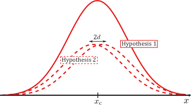
Figure 2: Intensity distribution at the image plane arising from two nearly coinciding incoherent light sources ($\sigma\gg d$) given an imaging system that exhibits a Gaussian point spread function (PSF). Due to the large overlap between the two PSFs, direct imaging does not allow to accurately estimate the positions of each source, and is incapable of discriminating whether the image is the result of one or two sources—Hypothesis 1 and Hypothesis 2 respectively.

In order to overcome the diffraction limit Tsang et al. Tsang et al. (2016) proposed to abandon direct imaging and count instead the number of photons in distinct spatial modes of light. In particular, when dealing with Gaussian PSFs the spatial modes can be interpreted as the energy eigenstates of the quantum mechanical harmonic oscillator, i.e., the Hermite-Gauss (HG) modes:

$$|\Phi_{n}(x_{R})\rangle=\frac{1}{\sqrt{2^{n}\,n!}}\frac{1}{\sqrt[4]{2\pi\,\sigma^{2}}}\times\int_{-\infty}^{\infty}e^{-\frac{(x-x_{R})^{2}}{4\sigma^{2}}}\,H_{n}\!\left(\frac{x-x_{R}}{\sqrt{2}\sigma}\right)\,|x\rangle\,\mathrm{d}x,$$ (12)

where

$$H_{n}(\alpha):=(-1)^{n}\,e^{\alpha^{2}}\frac{\mathrm{d}^{n}}{\mathrm{d}\alpha^{n}}\,e^{-\alpha^{2}}$$ (13)

are the Hermite polynomials, and $x_{R}$ is the reference position of the spatial modes. This measurement can be implemented with the help of linear optical pre-processing of the incoming radiation, followed by photon-number resolving detectors and can resolve two point sources no matter how close their PSFs are on the image plane so long as $x_{R}=x_{\mathrm{c}}$, i.e., the position of their centroid is known exactly. The latter can be estimated via direct imaging; its precision varies inversely proportionally with the square root of the measurement integration time Tsang et al. (2016). Moreover, even if the centroid is known sufficiently well, there is still the issue of perfectly aligning the measurement device for spatial mode demultiplexing, or SPADE for short, i.e., setting $x_{R}=x_{\mathrm{c}}$. A proposal on how best to accomplish this using a finite number of observations was proposed recently by Grace et al. Grace et al. (2020). There the authors proposed to combine direct imaging and SPADE techniques, in a two-stage procedure; the former uses part of the incoming radiation to adjust the exact position of the latter via a servo feedback mechanism in order to gradually reduce the misalignment, $\delta:=x_{\mathrm{c}}-x_{R}$ marked explicitly in Fig. 1, which is a priori not known.

In this work we take misalignment of the demultiplexing device as fact and determine the theoretical limits imposed by such misalignment in both estimation and discrimination tasks (see Fig. 2). To do so we allow ourselves the freedom of performing arbitrary, linear-optical post processing of the demultiplexed radiation. Specifically, we shall analytically determine how such linear-optical post processing, based on complete knowledge of the value of the misalignment, affects estimation precision, as well as the minimal resolvable distance. To do so we shall make use of an approximation of the state of the incoming radiation known as the qubit model Chrostowski et al. (2017), which we now review.

II.3 The qubit model for two incoherent point sources.

The qubit model is an approximation of the PSF in the presence of misalignment Chrostowski et al. (2017). The latter can be understood as performing the projective measurement of Eq. (12) about some reference position $x_{R}\neq x_{i}$ for $i\in(0,1,2)$. Assuming that this misalignment is small, i.e., $x_{R}\approx x_{i}$, we can Taylor expand the probability amplitudes of each source, $\Psi(x-x_{i}),\,i\in\{1,2\}$, about $x_{R}$ as follows:

$$\begin{split}|\Psi(x_{i})\rangle\approx&\int_{-\infty}^{\infty}\mathrm{d}x\,\Psi(x-x_{R})\,|x\rangle+(x_{i}-x_{R})\int_{-\infty}^{\infty}\mathrm{d}x\,\frac{\mathrm{d}\Psi(x-x_{i})}{\mathrm{d}x_{i}}\bigg{\rvert}_{x_{i}=x_{R}}|x\rangle\\ =:&\;|0\rangle-(x_{i}-x_{R})\sqrt{\mathcal{N}}|1\rangle,\end{split}$$ (14)

and identify a qubit subspace with $|0\rangle:=|\Psi(x_{R})\rangle$ and

$$|1\rangle:=\frac{-1}{\sqrt{\mathcal{N}}}\int_{-\infty}^{\infty}\mathrm{d}x\,\frac{\mathrm{d}\Psi(x-x_{i})}{\mathrm{d}x_{i}}\bigg{\rvert}_{x_{i}=x_{R}}|x\rangle$$ (15)

an orthonormal basis. Here, $\mathcal{N}$ is an appropriate normalisation factor which for the Gaussian and Sinc PSFs reads

$$\begin{split}\mathcal{N}_{\mathrm{G}}&=\frac{1}{4\sigma^{2}},\qquad\mathcal{N}_{\mathrm{S}}=\frac{\pi^{2}}{3\sigma^{2}},\end{split}$$ (16)

respectively.

The state of the incoming radiation can now be described, to a very good approximation, by the following qubit density operators, for one and two sources, respectively:

$$\rho^{(1)} \approx\frac{1}{1+(\sigma\theta)^{2}\mathcal{N}}\left(\begin{matrix}1&-\sigma\theta\sqrt{\mathcal{N}}\\ -\sigma\theta\sqrt{\mathcal{N}}&(\sigma\theta)^{2}\mathcal{N}\end{matrix}\right)$$

$$\rho^{(2)} \approx\frac{1}{1+\sigma^{2}(\theta^{2}+\epsilon^{2})\mathcal{N}}\left(\begin{matrix}1&-\sigma\theta\sqrt{\mathcal{N}}\\ -\sigma\theta\sqrt{\mathcal{N}}&\sigma^{2}(\theta^{2}+\epsilon^{2})\mathcal{N}\end{matrix}\right),$$ (17)

where we now introduced dimensionless parameters for misalignment and separation:

$$\theta:=\frac{\delta}{\sigma}=\frac{x_{\mathrm{c}}-x_{R}}{\sigma}\qquad\text{and}\qquad\epsilon:=\frac{d}{\sigma},$$ (18)

respectively. The qubit model allows us to visualise the effects of misalignment on a given PSF in terms of the Bloch representation of qubit density matrices, i.e.,

$$\rho:=\frac{{\mbox{$1{\bf l}$}}+\bm{{\bf r}}\cdot\bm{\sigma}}{2},$$ (19)

where $\bm{{\bf r}}\in\mathcal{R}_{3}$, has elements $\mathrm{r}_{i}=\mathrm{Tr}(\sigma_{i}\rho)$ and $\bm{\sigma}:=(\sigma_{1},\sigma_{2},\sigma_{3})^{T}$ is the vector of Pauli matrices $\sigma_{i}$. For the Gaussian and Sinc PSFs the corresponding Bloch vectors read

$${\bf r}^{(1)}_{\mathrm{G}} =\frac{1}{1+\frac{\theta^{2}}{4}}\left(\begin{matrix}-\theta\\ 0\\ 1-\frac{\theta^{2}}{4}\end{matrix}\right),\;{\bf r}^{(2)}_{\mathrm{G}}=\frac{1}{1+\frac{\theta^{2}+\epsilon^{2}}{4}}\left(\begin{matrix}-\theta\\ 0\\ 1-\frac{\theta^{2}+\epsilon^{2}}{4}\\ \end{matrix}\right)$$

$${\bf r}^{(1)}_{\mathrm{S}} \approx\frac{1}{1+\frac{\theta^{2}}{3}}\left(\begin{matrix}-\frac{2\theta}{\sqrt{3}}\\ 0\\ 1-\frac{\theta^{2}}{3}\end{matrix}\right),\;{\bf r}^{(2)}_{\mathrm{S}}\approx\frac{1}{1+\frac{\theta^{2}+\epsilon^{2}}{3}}\left(\begin{matrix}-\frac{2\theta}{\sqrt{3}}\\ 0\\ 1-\frac{\theta^{2}+\epsilon^{2}}{3}\end{matrix}\right),$$ (20)

respectively. Using the approximations

$$\begin{split}\frac{1}{1+x^{2}}&\approx 1-x^{2}\\ 1-\frac{(\theta^{2}+\epsilon^{2})}{2}&\approx(1-\frac{\theta^{2}}{2})(1-\frac{\epsilon^{2}}{2})\approx\cos\theta\left(1-\frac{\epsilon^{2}}{2}\right),\end{split}$$ (21)

and keeping terms up to second order, $\mathcal{O}(\theta^{i}\epsilon^{j})$ with $i+j=2$, the Bloch vectors in Eq. (20) can be further approximated by

$${\bf r}^{(1)}_{\mathrm{G}} \approx\left(\begin{matrix}-\sin\theta\\ 0\\ \cos\theta\end{matrix}\right),\quad{\bf r}^{(2)}_{\mathrm{G}}\approx\left(1-\frac{\epsilon^{2}}{2}\right)\left(\begin{matrix}-\sin\theta\\ 0\\ \cos\theta\end{matrix}\right)$$

$${\bf r}^{(1)}_{\mathrm{S}} \approx\left(\begin{matrix}-\sin\frac{2\theta}{\sqrt{3}}\\ 0\\ \cos\frac{2\theta}{\sqrt{3}}\end{matrix}\right),\quad{\bf r}^{(2)}_{\mathrm{S}}\approx\left(1-\frac{\epsilon^{2}}{2}\right)\left(\begin{matrix}-\sin\frac{2\theta}{\sqrt{3}}\\ 0\\ \cos\frac{2\theta}{\sqrt{3}}\end{matrix}\right).$$ (22)

Consequently the misalignment, $\theta$, can be understood as an infinitesimal rotation about the $y$-axis in the Bloch-sphere picture, whereas the separation, $\epsilon$, between the centres of the two incoherent point sources affects the purity of the state Chrostowski et al. (2017).

Our aim is to use the qubit model to study the effects of misalignment, both in the estimation of the separation between two point sources, as well as in the task of discriminating between the single and two source hypotheses. We begin first with estimating the separation between two incoherent point sources.

III Separation estimation under misalignment

In this section we review the quantum information tools for multi-parameter estimation, after which we use the qubit model to derive the optimal measurement for estimating the separation between two incoherent point sources under misalignment.

III.1 Classical and quantum statistical inference

The task at hand is the estimation of two parameters: the two sources centroid position $x_{\mathrm{c}}$, and their separation $d$ from a finite sample of $n$ measurement outcomes $\bm{y}:=(y_{1},\ldots,y_{n})^{T},\,y_{i}\in\mathbb{R}$, in one dimension . For ease of notation let us denote the parameters to be estimated by $\bm{\lambda}:=(\lambda_{1},\lambda_{2})^{T}\in\mathbb{R}^{2}$. Then the data constitutes a random variable $\bm{y}\in\bm{Y}$ distributed according to $p(\bm{y}|\bm{\lambda})$.

An estimator, $f_{i}:\bm{Y}\to\mathbb{R}$, is any function that maps every possible measurement record to an estimate $\hat{\lambda}_{i}=f_{i}(\bm{y})$ of the parameter $\lambda_{i}$. An estimator is said to be unbiased if $\langle\hat{\lambda}_{i}\rangle:=\sum_{\bm{y}}p(\bm{y}|\bm{\lambda})\hat{\lambda}_{i}=\lambda_{i}$. Denoting by $\hat{\bm{\lambda}}\in\mathbb{R}^{2}$ the two-dimensional vector of estimates of $\bm{\lambda}$, the Cramér-Rao inequality places a lower bound on the covariance matrix of any unbiased estimator Cramér (1961) :

$$\left\langle\left(\hat{\bm{\lambda}}-\bm{\lambda}\right)\cdot\left(\hat{\bm{\lambda}}-\bm{\lambda}\right)^{T}\right\rangle\geq\left(n\,\bm{F}\left(p(\bm{y}|\bm{\lambda})\right)\right)^{-1},$$ (23)

where $\bm{F}\left(p(\bm{y}|\bm{\lambda})\right)$ is the Fisher information matrix Fisher (1922)

$$F_{ij}(p(\bm{y}|\bm{\lambda})):=\left\langle\left(\frac{\partial\,\ln p(\bm{y}|\bm{\lambda})}{\partial_{\lambda_{i}}}\right)\left(\frac{\partial\,\ln p(\bm{y}|\bm{\lambda})}{\partial_{\lambda_{j}}}\right)\right\rangle,$$ (24)

quantifying the amount of information the random variable $\bm{Y}$ carries about the parameters $\bm{\lambda}$.

An estimator is said to be efficient if it saturates the inequality of Eq (23). Note that it is possible that no efficient estimator exists if the data sample is finite. However, for an asymptotically large sample size, i.e., $n\to\infty$, it can be shown that the maximum likelihood estimator always saturates the Cramér-Rao bound Wilks (1962).

In quantum statistical inference the random variable $\bm{Y}$ and its corresponding probability distribution $p(\bm{y}|\bm{\lambda})$ arise from performing a quantum measurement on a quantum system. Any set of positive operators, $\{E_{\bm{y}}\geq 0\,;\,{\bm{y}}\in{\bm{Y}}\}$, satisfying the completeness relation $\sum_{\bm{y}\in Y}E_{\bm{y}}={\mbox{$1{\bf l}$}}$ is an admissible measurement, termed a Positive Operator Valued Measure, or POVM for short. By virtue of positivity $E_{\bm{y}}=M^{\dagger}_{\bm{y}}\,M_{\bm{y}}$, where $M_{\bm{y}}$ constitute one of the infinitude of square roots of $E_{\bm{y}}$. If $M_{\bm{y}}=M^{\dagger}_{\bm{y}}$ and $M_{\bm{y}}^{2}=M_{\bm{y}}$ then the POVM consists of projective operators, and there exists a dynamical variable—energy, position, (angular) momentum, etc.—represented by the Hermitian operator $O$, such that $O=\sum_{\bm{y}}\mu_{\bm{y}}\,M_{\bm{y}}$. Given a POVM the conditional probability of obtaining a given measurement record $\bm{y}$ is given by

$$p(\bm{y}|\bm{\lambda})=\mathrm{Tr}\left(E_{\bm{y}}\rho(\bm{\lambda})\right).$$ (25)

Using the natural Riemannian geometry of the space of bounded, positive linear operators one can define the operator analogue of the logarithmic derivative in Eq. (24) for each parameter $\lambda_{i}$—the symmetric logarithmic derivative (SLD), $\mathcal{L}_{\lambda_{i}}$—as the solution to

$$\frac{\partial\,\rho(\bm{\lambda})}{\partial_{\lambda_{i}}}:=\frac{1}{2}\left(\mathcal{L}_{\lambda_{i}}\rho(\bm{\lambda})+\rho(\bm{\lambda})\mathcal{L}_{\lambda_{i}}\right).$$ (26)

In the eigendecomposition of $\rho(\bm{\lambda)}$, $\{\mu_{j},\,|\psi_{j}\rangle\}$, the SLD operator $\mathcal{L}_{\lambda_{i}}$ is explicitly given by Helstrom (1976); Holevo (1982)

$$\mathcal{L}_{\lambda_{i}}=2\sum_{\begin{subarray}{c}\alpha,\beta\\ \mu_{\alpha}+\mu_{\beta}\neq 0\end{subarray}}\frac{\langle\psi_{\alpha}(\bm{\lambda})|\partial_{\lambda_{i}}\rho_{\bm{\lambda}}|\psi_{\beta}(\bm{\lambda})\rangle}{\mu_{\alpha}(\bm{\lambda})+\mu_{\beta}(\bm{\lambda})}|\psi_{\alpha}(\bm{\lambda})\rangle\langle\psi_{\beta}(\bm{\lambda})|,$$ (27)

and the quantum Fisher information matrix elements read

$$\bm{\mathcal{F}}_{ij}(\rho(\bm{\lambda}))=\frac{1}{2}\mathrm{Tr}\left(\rho_{\bm{\lambda}}\left\{\mathcal{L}_{\lambda_{i}},\mathcal{L}_{\lambda_{j}}\right\}\right),$$ (28)

where $\{A,B\}=AB+BA$. We thus have the following chain of inequalities for the covariance matrix

$$\left\langle\left(\hat{\bm{\lambda}}-\bm{\lambda}\right)\cdot\left(\hat{\bm{\lambda}}-\bm{\lambda}\right)^{T}\right\rangle \geq(n\,\bm{F}\left(p(\bm{y}|\bm{\lambda})\right))^{-1}$$

$$\geq(n\,\bm{\mathcal{F}}\left(\rho(\bm{\lambda})\right))^{-1},$$ (29)

the latter inequality commonly referred to as the quantum Cramér-Rao bound.

For each single parameter $\lambda_{i}$ an asymptotically efficient estimator exists and is given by the maximum likelihood estimator of the POVM whose elements are the eigenprojectors of the corresponding SLD operator. If all these operators commute, i.e., $[\mathcal{L}_{\lambda_{i}},\,\mathcal{L}_{\lambda_{j}}]=0,\,\forall\,i\neq j$, then the quantum Cramer-Rao bound is asymptotically achievable. Note that commutativity is only a sufficient condition; a necessary and sufficient condition—assuming asymptotically many independent and identically distributed copies ($n\gg 1$) of $\rho(\bm{\lambda})$—is $\mathrm{Tr}\left(\rho(\bm{\lambda})\left[\mathcal{L}_{\lambda_{i}},\,\mathcal{L}_{\lambda_{j}}\right]\right)=0,\,\forall\,i\neq j$ Ragy et al. (2016). However, note that the POVM that saturates the quantum Cramer-Rao bound in Eq. (29) may, in general, correspond to a collective measurement on all the $n\gg 1$ copies Demkowicz-Dobrzański et al. (2020); Albarelli et al. (2020).

Hitherto, the application of super-resolving measurements in imaging has focused primarily on “beating” the diffraction limit and maximising the precision in estimating the sources separation, $2d$, while assuming full control over all other parameters, in particular, the centroid’s position, $x_{\mathrm{c}}$. Of particular importance is the fact that the measurement that attains the quantum Fisher information when estimating only the separation between two incoherent point sources is a projective measurement that does not depend on knowing $d$ in advance Tsang et al. (2016). It does, however, require perfect knowledge of the centroid, $x_{\mathrm{c}}$, of the PSF as well as perfect positioning of SPADE so that any misalignment, $\delta\propto\theta$ in Equation (18), can always be set to zero.

The separation can be estimated without requiring any knowledge about the centroid, if one has access to a quantum memory with a long coherence time so as to store photons collected during several independent experimental rounds ($n>1$) and be able to implement collective measurements Ragy et al. (2016). A proof-of-principle experiment that makes use of a measurement on a doublet of photons ($n=2$) and allows for simultaneous estimation of both the centroid and the separation of the sources has been reported recently Parniak et al. (2018). This has been achieved by encoding the spatial distribution of two incoherent sources into the spatial profile of a single photon generated in the laboratory. Utilising a pair of such photons and interfering them as in the the Hong-Ou-Mandel experiment Hong et al. (1987), the information about both separation and centroid parameters can be harmlessly retrieved, while estimating the former with precision beyond the diffraction limit Parniak et al. (2018). On the other hand, a recent theoretical study has proposed the use of direct imaging and SPADE techniques in parallel Grace et al. (2020). Direct imaging is performed repeatedly to part of the incoming radiation adjusting the exact position of SPADE via a servo feedback mechanism, in order to gradually reduce the misalignment, $\theta$ in Eq. (18), with increasing number of experimental repetitions.

In the next subsection we use the qubit model to obtain the optimum measurement strategy for estimating the separation between two incoherent sources in presence of misalignment.

III.2 Separation estimation under misalignment in the qubit approximation

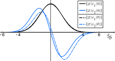
Figure 3: Spatial representation of the ROTADE operators for aligned (solid line, $\theta=0$) and misaligned (dot- dashed, $\theta=0.4$) measurement. The plots are given for $\frac{d}{\sigma}=0.25$. $|\psi_{\alpha}(\theta)\rangle$ is defined in Eq. (30).

Assuming the separation between the incoherent sources to be small—as assured in the super-resolution regime—we use the qubit model in order to construct the optimal measurement for estimating the separation between two point sources under misalignment. We begin by first considering the Gaussian PSF. The eigenvalues and corresponding eigenvectors of $\rho^{(2)}_{\mathrm{G}}$ are

$$\begin{split}\mu_{1}(\epsilon)=\frac{\epsilon^{2}}{4},\quad&|\psi_{1}(\theta)\rangle=\sin\frac{\theta}{2}|0\rangle+\cos\frac{\theta}{2}|1\rangle\\ \mu_{2}(\epsilon)=1-\mu_{1}(\epsilon),\quad&|\psi_{2}(\theta)\rangle=-\cos\frac{\theta}{2}|0\rangle+\sin\frac{\theta}{2}|1\rangle.\end{split}$$ (30)

Using Eq. (27) the corresponding SLD operators are, in the eigenbasis $\{|\psi_{1}(\theta)\rangle,|\psi_{2}(\theta)\rangle\}$:

$$\mathcal{L}_{\theta} =\left(1-\frac{\epsilon^{2}}{2}\right)\sigma_{x},\qquad\mathcal{L}_{\epsilon}=\left(\begin{matrix}\frac{2}{\epsilon}&0\\ 0&\frac{2\epsilon}{\epsilon^{2}-4}\end{matrix}\right).$$ (31)

Observe that $[\mathcal{L}_{\theta},\mathcal{L}_{\epsilon}]\neq 0$, meaning that the optimal measurements for each of these parameters are incompatible. However, $\mathrm{Tr}\left(\rho^{(2)}_{\mathrm{G}}[\mathcal{L}_{\theta},\mathcal{L}_{\epsilon}]\right)=0$, which implies that there exists a possibly joint measurement on all $n$ photons that saturates the quantum Cramér-Rao bound given by

$$\langle(\hat{\theta}-\theta,\hat{\epsilon}-\epsilon)^{T}(\hat{\theta}-\theta,\hat{\epsilon}-\epsilon)\rangle\geq\frac{1}{n}\left(\begin{matrix}\frac{1}{1-\epsilon^{2}}&0\\ 0&\frac{1}{1+\frac{\epsilon^{2}}{4}}\end{matrix}\right).$$ (32)

The eigenvectors of the SLD operators (Eq. (31)) are given by

$$|\theta_{\pm}\rangle =\frac{1}{\sqrt{2}}\left(\left(\sin\frac{\theta}{2}\pm\cos\frac{\theta}{2}\right)|0\rangle+\left(\sin\frac{\theta}{2}\mp\cos\frac{\theta}{2}\right)|1\rangle\right),$$ (33)

$$|\epsilon_{\alpha}\rangle =|\psi_{\alpha}(\theta)\rangle\quad\text{with}\quad\alpha\in\{1,2\},$$ (34)

respectively. As $\mathcal{L}_{\epsilon}$ is a diagonal operator, the optimal measurement in Eq. (34) for estimating the re-scaled separation $\epsilon$ between the two sources according to the qubit model is simply given by a projective measurement in the eigenbasis of Eq. (30). Henceforth, we shall refer to this measurement as the rotated mode demultiplexer (ROTADE), i.e. the detection scheme depicted schematically in Fig. 1 with the rotation $R(\delta)$ adequately adjusted to $\delta=\theta\sigma$.

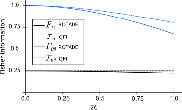
Figure 4: Gaussian aperture: Quantum Fisher information, $\frac{\mathcal{F}_{\bm{\lambda}}}{n}$, attained in Tsang et al. (2016) (dashed lines) and classical Fisher information associated to the ROTADE measurement $\frac{F_{\bm{\lambda}}}{n}$ (solid lines), for separation $\epsilon$ (red) and misalignment $\theta$ (blue) parameters for perfect alignment $\theta=0$, as a function of $2\epsilon$. As the POVM Eq. 34 is derived based on the qubit model, it ceases to be optimal with increasing separation of the sources (here for $\epsilon\lesssim 0.1$).

In order to compare the quality of the ROTADE measurement, we use Eq. (14) to map the measurement operators into their position-based representation. The latter are shown in Fig. 3. One can then explicitly determine the probability distribution arising from these measurements and hence the corresponding Fisher information using Eq. (24). The results are shown in Fig. 4, where we compare the performance of ROTADE with the quantum Fisher information Tsang et al. (2016) for $\theta=0$, i.e. in the absence of misalignment. We see that up to separations $\epsilon=\frac{d}{\sigma}\lesssim 0.5$ the Fisher information of ROTADE drops to $\approx 90\%$ of the optimal value. On the other hand, up to $\epsilon=\frac{d}{\sigma}\lesssim 0.1$ ROTADE maintains its optimality, emphasising that the qubit model approximates well the super-resolution problem in this regime. Hence, in the limit where the qubit model holds, counting photons only in the first two HG modes suffices to estimate the separation.

A simpler measurement that also achieves the quantum bound (Fig. 4) is B-SPADE Tsang et al. (2016). This is a coarse grained version of SPADE where only photons in the fundamental HG mode of SPADE are counted, while lumping all other modes to produce a single photon-count outcome. As the probability of detecting the zeroth HG mode occurs regardless of the separation, $d$, B-SPADE is more experimentally friendly, but suffers in the same manner as SPADE from the misalignment problem. In Fig. 5 we compare the performance of ROTADE with B-SPADE in estimating the separation under a misalignment $\theta\leq 0.5$.

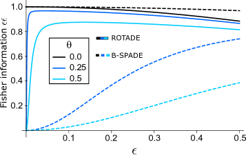
Figure 5: Gaussian aperture: B-SPADE Fisher information attained in Tsang et al. (2016) (dashed lines) and ROTADE Fisher information (solid lines) for separation estimation under misalignment, $\frac{F_{\epsilon\epsilon}}{n}$, as a function of the separation.

In order to capture the difference between the aforementioned measurements we compare the Taylor expansions of their corresponding Fisher information up to first non-trivial order, for small separation $\epsilon$. These are given by

$$\begin{split}F^{(\mathrm{R})}_{\bm{\epsilon\epsilon}}(\epsilon)&\approx\epsilon^{2}C^{(R)}(\theta)\\ F^{(\mathrm{B})}_{\bm{\epsilon\epsilon}}(\epsilon)&\approx\epsilon^{2}C^{(B)}(\theta),\end{split}$$ (35)

where $C^{(R)}(\theta),\,C^{(B)}(\theta)$ are coefficients pertaining to the measurements themselves and depend only on the misalignment $\theta$ (notably they are independent of $n$ and $\epsilon$). The behaviour of these coefficients governs the precise minimal resolvable distance for each measurement as we now explain.

The signal-to-noise-ratio $\epsilon/\Delta\epsilon$ can be expressed as

$$\epsilon\sqrt{nF^{(\mathrm{\#})}_{\bm{\epsilon\epsilon}}(\epsilon)}\geq 1,$$ (36)

where $\#\in(R,B)$. The minimal resolvable separation, $\epsilon^{(\#)}_{\min}(\theta)$, for each measurement is defined as that $\epsilon$ in Eq. (36) for which equality holds. Using the approximations of Eq. (35) one obtains

$$\epsilon^{(\#)}_{\min}(\theta)=\frac{1}{\sqrt[4]{nC^{(\#)}(\theta)}}.$$ (37)

Taylor expanding the functions $C^{(\#)}(\theta)^{-1}$ to first non-trivial order in $\theta$ one obtains

$$\begin{split}C^{(\mathrm{R})}(\theta)^{-1}&\approx\frac{\theta^{6}}{12^{2}}\\ C^{(\mathrm{B})}(\theta)^{-1}&\approx\theta^{2}.\end{split}$$ (38)

It follows that

$$\begin{split}\epsilon^{(\mathrm{R})}_{\min}(\theta)&\approx\frac{1}{\sqrt[4]{n}}\frac{\theta^{\frac{3}{2}}}{\sqrt{12}}\\ \epsilon^{(\mathrm{B})}_{\min}(\theta)&\approx\frac{\sqrt{\theta}}{\sqrt[4]{n}},\end{split}$$ (39)

where $\epsilon_{\min}(\theta)\propto n^{-\frac{1}{4}}$ is a consequence of $F_{\bm{\epsilon\epsilon}}\propto\epsilon^{2}$ in Eq. (35). In contrast, observe that in the ideal case of no misalignment, for which $F_{\bm{\epsilon\epsilon}}\propto 1$, the minimal resolvable distance scales as $\epsilon_{\min}(0)\propto n^{-\frac{1}{2}}$.

The quadratic increase in the scaling of $\epsilon_{\min}$ for both ROTADE and B-SPADE due to misalignment mimicks closely the behaviour of cross-talk between the measurement modes addressed recently by Guessner et al. Gessner et al. (2020). As our qubit approximation puts us in the regime of only monitoring the first two HG modes, and misalignment corresponds to a unitary rotation of the latter, it follows that this unitary rotation can be interpreted as the cross-talk matrix of Gessner et al. (2020). As the cross-talk probability between the two modes is proportional to $\sin^{2}\theta\approx\theta^{2}$, $\epsilon^{(B)}_{\min}$ of Eq. (39) follows precisely the analytical model for uniform cross-talk of Gessner et al. (2020).

Our results show that super-resolution is impossible if the initial demultiplexing of the incoming radiation suffers any misalignment, even if the latter is known. Nevertheless, cross-modulation techniques between the two primary HG modes can help in significantly reducing the minimum resolvable distance.

In Appendix A we obtain the optimal measurement under misalignment for the Sinc PSF, as well as the minimum resolvable distance. Our results confirm the efficacy of the qubit model; for whatever PSF the first two modes are the most relevant ones in estimating the position of light sources with separation well below the diffraction limit. In the next section, we will discuss how the optimal measurement under misalignment derived using the qubit model is also optimal for the task of discriminating whether the incoming radiation is due to two incoherent point sources or one source with twice the power under misalignment.

IV Classical and quantum state discrimination: one or two point sources.

Hitherto our focus was to estimate the relevant parameters of two incoherent point sources. However, a more pertinent question is whether the incoming radiation is due to two incoherent point sources very close together (the two source hypothesis, $H^{(2)}$), or one point source with twice the power (the one source hypothesis, $H^{(1)}$). To that end we first review the fundamentals of classical and quantum decision theory and, in particular, simple binary hypothesis testing Helstrom (1976); Holevo (1982). We then apply these tools to optimally discriminate between $H^{(1)},\,H^{(2)}$ in the presence of misalignment and compare the performance of ROTADE with measurements in the literature, showing that our measurement outperforms all the latter.

IV.1 Classical and quantum hypothesis testing

A fundamental problem in decision theory is to discriminate among several possible hypothesis based on a number, $n$, of observations. The simplest such scenario—known as binary hypothesis testing—occurs when there are two hypothesis, $H^{(1)},\,H^{(2)}$ that need to be discriminated. For simplicity, assume that each observation consists of a finite set of possible outcomes $y\in Y$ . Under hypothesis $H^{(i)}$, these outcomes are distributed according to $p(y|H^{(i)})$, and thus the problem becomes one of determining from which probability distribution the random variable $Y$ is drawn.

For a single observation ($n=1$) let $f:Y\to\{H^{(1)},\,H^{(2)}\}$ be a decision rule. Under such a decision rule the probability of making an error based on a single observation is

$$P_{\mathrm{err}}=\frac{1}{2}\Big{(}p\left(f(y)=H^{(2)}|H^{(1)}\right)+p\left(f(y)=H^{(1)}|H^{(2)}\right)\Big{)},$$ (40)

where we have assumed that each hypothesis is equally likely. The conditional probabilities $p\left(f(y)=H^{(2)}|H^{(1)}\right),\,p\left(f(y)=H^{(1)}|H^{(2)}\right)$ are the type-1 (mistaking one source for two) and type-2 (mistaking two sources for one) errors, respectively. For binary hypothesis testing, the optimal decision rule is to assign the hypothesis with the highest posterior distribution Rényi (1966); Neyman and Pearson (1933) which, for equally likely hypothesis, translates to

$$f(y)=\begin{cases}H^{(1)}&\mathrm{if}\quad p\left(y|H^{(1)})>p(y|H^{(2)}\right)\\ H^{(2)}&\mathrm{if}\quad p\left(y|H^{(2)})>p(y|H^{(1)}\right)\\ \mathrm{any}&\mathrm{if}\quad p\left(y|H^{(1)})=p(y|H^{(2)}\right),\end{cases}$$ (41)

and the corresponding probability of error reads

$$P_{\mathrm{err}} =\sum_{y\in Y}p(y)\,\mathrm{min}\left\{p\left(H^{(i)}|y\right)\right\}$$

$$=\sum_{y\in Y}\mathrm{min}\left\{p\left(y,H^{(i)}\right)\right\}$$

$$=\frac{1}{2}\left(1-\frac{1}{2}\sum_{y\in Y}\bigg{\lvert}\,p\left(y|H^{(1)}\right)-p\left(y|H^{(2)}\right)\bigg{\rvert}\right)$$ (42)

where we have made use of the identity $\mathrm{min}\{a,b\}=\frac{1}{2}\left(a+b-\lvert a-b\rvert\right)$ in order to obtain the last equality.

Quantum hypothesis testing now follows by noting that $p\left(y|H^{(i)}\right)=\mathrm{Tr}\left(E_{y}\,\rho^{(i)}\right)$ where $\{E_{y}\}$ constitute a POVM and the hypothesis, $\rho^{(i)},\,i\in(1,2)$, are given by Eqs. (8, 9). Doing the appropriate substitutions in Eq. (42) one obtains

$$P_{\mathrm{err}}=\frac{1}{2}\left(1-\frac{1}{2}\mathrm{Tr}\left(\sum_{y\in Y}E_{y}\bigg{\lvert}\rho^{(1)}-\rho^{(2)}\bigg{\rvert}\right)\right).$$ (43)

Unlike the classical case, in quantum binary hypothesis testing we are free to choose among all admissible POVMs the one that yields the smallest probability of error. The optimal measurement in this case was derived by Helstrom Helstrom (1976) and corresponds to a two outcome measurement $\{E_{0},\,E_{1}\}$ on the positive and negative eigenspaces of the operator

$$\Gamma:=\frac{1}{2}\left(\rho^{(2)}-\rho^{(1)}\right).$$ (44)

Given $n$ copies of the initial state, the Helstrom measurement is generally a collective measurement on the positive and negative eigenspaces of $\Gamma^{\otimes n}=\frac{1}{2}\left(\rho^{(2)\otimes n}-\rho^{(1)\otimes n}\right)$. For clarity we shall call the single copy optimal measurement as the Helstrom measurement, and the overall optimal measurement on $n$ copies as the collective Helstrom measurement.

The probability of error decreases exponentially with the number of copies $n$. In order to compare the performance of different measurement strategies one needs to determine the rate at which this error probability decreases. For an asymptotically large ($n\rightarrow\infty$) number of observations the probability of error saturates Chernoff’s inequality Chernoff (1952):

$$P_{\mathrm{err}}(n)\leq e^{-n\xi},$$ (45)

where,

$$\xi:=-\log\min_{0\leq s\leq 1}\sum_{y\in Y}p\left(y|H^{(1)}\right)^{s}p\left(y|H^{(2)}\right)^{1-s}$$ (46)

is the Chernoff exponent. In the case of quantum hypothesis testing, the asymptotic error rate is given by the quantum Chernoff exponent Audenaert et al. (2007):

$$\xi\leq\xi^{(QM)}:=-\log\min_{0\leq s\leq 1}\mathrm{Tr}\!\left\{\left(\rho^{(1)}\right)^{s}\left(\rho^{(2)}\right)^{1-s}\right\},$$ (47)

which is generally larger than its classical counterpart. Note that the quantum Chernoff exponent only depends on the quantum states to be discriminated, and is independent of the measurement performed. Nonetheless, the inequality in Eq. (45) is asymptotically achievable in the limit of infinite copies. In this limit, $\xi$ reaches the ultimate quantum bound $\xi^{(QM)}$ of asymptotic (symmetric) hypothesis testing Nussbaum and Szkoła (2009). However, such attainability may require a collective Helstrom measurement to be performed on all the $n\to\infty$ copies.

Surprisingly, it was already Helstrom Helstrom (1973) who first addressed the problem of discriminating one-vs-two incoherent point sources of light with tools from hypothesis testing, and derived a sub-optimal measurement that; (i) lacks a physical realisation and (ii) requires knowledge of the separation of the two sources. Krovi et al. Krovi et al. (2016) derived the optimal quantum mechanical measurement that achieves the quantum Chernoff bound for the case where the separation of the two point sources is known and showed how to experimentally implement it. Shortly after, Lu et al. (2018) showed that the B-SPADE measurement of Tsang et al. (2016) achieves the quantum Chernoff bound for one-vs-two sources of arbitrary separation. However, just like in the estimation case, all these works assumed that the centre of the single source, as well as the centroid of the two source hypothesis, to be perfectly aligned with the demultiplexing measurements and neglected any noise at the detectors.

In the next subsection we analyse the behaviour of B-SPADE under misalignment and show that it falls short of the quantum optimal Chernoff bound. Using the qubit model we derive an alternative measurement strategy that is also sub-optimal but outperforms the B-SPADE under misalignment by far.

IV.2 State discrimination in the qubit approximation—the Helstrom measurement

Our aim is to determine whether the PSF observed at the misaligned imaging system is due to two incoherent point sources of equal intensities or a single source with twice the intensity. For the remainder of this section, we shall work with the Gaussian PSF (results for the Sinc PSF can be derived in a similar fashion and are presented in Appendix B). Using the qubit model the matrix $\Gamma$ of Eq. (44) can be explicitly computed to be

$$\Gamma=\frac{1}{4}\begin{pmatrix}-\cos\theta_{\mathrm{0}}-\frac{1}{2}\cos\theta_{\mathrm{c}}(\epsilon^{2}-2)&\sin\theta_{\mathrm{0}}+\frac{1}{2}\sin\theta_{\mathrm{c}}(\epsilon^{2}-2)\\ \\ \sin\theta_{\mathrm{0}}+\frac{1}{2}\sin\theta_{\mathrm{c}}(\epsilon^{2}-2)&\cos\theta_{\mathrm{0}}+\frac{1}{2}\cos\theta_{\mathrm{c}}(\epsilon^{2}-2)\end{pmatrix},$$ (48)

where $\theta_{\mathrm{0}}=\frac{x_{\mathrm{0}}-x_{R}}{\sigma}$ is the misalignment relative to the centre of a single source PSF, $\theta_{\mathrm{c}}=\frac{x_{\mathrm{c}}-x_{R}}{\sigma}$ is the misalignment relative to the centroid, $x_{\mathrm{c}}$, of the two sources PSF, and $\epsilon$ is defined as in Eq. 18. Notice that, in principle, the centre of a single source need not coincide with the centroid of two sources, nor with the position of the demultiplexing measurement, $x_{\mathrm{0}}\neq x_{\mathrm{c}}\neq x_{R}\quad(\theta_{\mathrm{0}}\neq\theta_{\mathrm{c}})$. Nonetheless, hereafter we shall restrict our analysis to the case where only the demultiplexing measurements are misaligned, hence we will define:

$$\theta:=\theta_{\mathrm{0}}=\theta_{\mathrm{c}}.$$ (49)

In this regime, the Helstrom measurement is independent of separation and is equivalent to ROTADE.

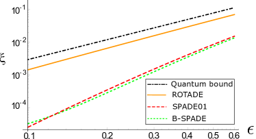
Figure 6: Numerical optimisation of the Chernoff exponent under misalignment as a function of the separation in $\log-\log$ plot, for $x_{R}=0.4$ and $\sigma=1$.

In case the detector and centroid are perfectly aligned, $\theta=0$, ROTADE is only the projection onto the zeroth and first HG modes. We shall refer to this measurement as SPADE$01$, in order to distinguish it from B-SPADE which projects only on the zeroth mode. We remark that all measurement strategies reach the quantum bound for zero misalignment. The main advantages of SPADE$01$ for aligned measurement device are: it is independent of the two-sources separation, the need to count photons only in the first two HG modes (photons coupling to higher modes correspond to no-clicks and are insignificant to the measurement statistics), and the unambiguous two-source discrimination whenever a photon is detected in the first HG mode. These results are shown in Appendix C.

Measurement	$p(f(y)=H^{(2)}|H^{(1)})$	$p(f(y)=H^{(1)}|H^{(2)})$
ROTADE	$\frac{\theta^{6}}{576\sigma^{6}}$	$\exp{\left(-\frac{d^{2}}{4\sigma^{2}}\right)}\left(1-\frac{d^{2}\theta^{2}}{16\sigma^{4}}\right)$
SPADE01	$\frac{\theta^{2}}{4\sigma^{2}}$	$\exp{\left(-\frac{d^{2}}{4\sigma^{2}}\right)}\left(1+\frac{(d^{2}-2\sigma^{2})\theta^{2}}{8\sigma^{4}}\right)$
B-SPADE	$\frac{d^{2}\theta^{2}\operatorname{csch}\left(\frac{d^{2}}{4\sigma^{2}}\right)}{16\sigma^{4}}$	$\exp{\left(-\frac{d^{2}}{4\sigma^{2}}\right)}\left(1+\frac{(d^{2}-2\sigma^{2})\theta^{2}}{8\sigma^{4}}\right)$

Table 1: Taylor expansion to the first non-trivial order in $\theta$ for the $type-1$ (second column) and $type-2$ (third column) error probabilities for ROTADE, SPADE$01$ and B-SPADE.

Table 1 shows how the one shot error probability scales as a function of the misalignment for the first non-trivial order of the Taylor expansion around $\theta=0$. Notice that for ROTADE, the $type-1$ error, responsible for the unambiguous determination of the two-source hypothesis, is four orders of magnitude smaller compared to that of SPADE$01$ and B-SPADE. Hence in the single-shot scenario ROTADE significantly outperforms both these measurements.

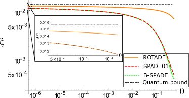
Figure 7: Numerical determination of the Chernoff exponent as a function of the misalignment, for separation $\epsilon=0.25$ between a pair of sources with $\sigma=1$. The inset shows how the Chernoff exponent varies for the three relevant measurement strategies for $\theta\approx 0$.

The Chernoff exponent of the SPADE$01$ measurement under misalignment behaves similarly to that of B-SPADE, the asymptotic results of all measurement strategies under misalignment as function of separation are represented in Fig. 6. However, in contrast with the aligned scenario, for $\theta\neq 0$ the probability of detecting photons into higher HG modes is non-negligible, and corresponds to the no-click probability. This probability represents the intrinsic error of the qubit model and it increases with misalignment (for details see Appendix C).

Unfortunately, we are unable to obtain an analytic expression for the Chernoff exponent under misalignment for any of the three strategies. This is because the $s$ that minimises the Chernoff exponent in Eq. 46 explicitly depends on $\theta$. Fig. 7 presents a numerical optimisation for the Chernoff exponent as a function of the misalignment. We observe that for all $\theta>0$ ROTADE outperforms both SPADE$01$ and B-SPADE, which is to be expected as ROTADE includes the knowledge on the amount of misalignment. Nonetheless, for exactly $\theta=0$ all the corresponding Chernoff exponents coincide with the quantum bound, what manifests their discontinuity as $\theta\to 0_{+}$.

V Conclusions

In this work we have analysed the impact of a de facto misalignment in the demultiplexing measurements of an optical imaging system in both estimating the separation of incoherent light sources, as well as discriminating between one-versus-two incoherent point sources. By allowing for linear-optical post processing of the two dominant demultiplexed modes, we have shown that super-resolution cannot be perfectly restored, even if the value of the misalignment is a priori known. Using quantum information methods, we have constructed misalignment-dependent strategies that, in the case of estimation, allow for subdiffraction-limited estimation of the separation of two incoherent light sources and analytically determined the dependence of both the estimation precision as well as the minimal resolvable distance as a function of the misalignment. Remarkably, the same measurement exhibits improved performance also in the task of discriminating among the one-vs-two source hypothesis showing significant improvement in both the single-shot as well as asymptotic probability of error.

Several interesting questions still remain. How does misalignment affect estimation precision when both the separation as well as the relative intensities of the two incoherent point sources need to be estimated? In the case of discrimination an interesting question occurs when the centres of the two hypothesis do not coincide, i.e., $x_{0}-x_{\mathrm{c}}\ll\sigma^{2}$ but neither $x_{0}$ nor $x_{\mathrm{c}}$ coincides with $x_{R}$. Then, the optimal Helstrom measurement does depend on knowing the separation between the two sources and it remains an open question if there exists a classical measurement with super-resolving power. We hope to answer these questions in the future.

Appendix

Appendix A Estimating the separation between Sinc-Bessel modes under misalignment

In this appendix section, we present the results of estimating the separation between two incoherent point sources imaged by a system with a rectangular aperture. The PSF of such a system is given by the Sinc function (see Eq. (7b)).

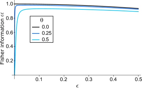
Figure 8: Rectangular aperture: $\frac{\mathcal{F}_{\epsilon\epsilon}}{n}$ for the equivalent to ROTADE measurement, as a function of separation for a rectangular aperture with $\sigma=1$ for different misalignments.

Repeating the calculation in Section III.1 the eigenvalues and corresponding eigenvectors of $\rho^{(2)}_{\mathrm{S}}$ are:

$$\begin{split}\mu_{1}(\epsilon)=\frac{\epsilon^{2}}{3},\quad&|\psi_{1}(\theta)\rangle=\sin\frac{\theta}{\sqrt{3}}|0\rangle+\cos\frac{\theta}{\sqrt{3}}|1\rangle\\ \mu_{2}(\epsilon)=1-\mu_{1}(\epsilon),\quad&|\psi_{2}(\theta)\rangle=-\cos\frac{\theta}{\sqrt{3}}|0\rangle+\sin\frac{\theta}{\sqrt{3}}|1\rangle,\end{split}$$ (50)

and using Eq. (27) the corresponding SLD operators are, in the eigenbasis $\{|\psi_{1}(\theta)\rangle,|\psi_{2}(\theta)\rangle\}$ are given by

$$\mathcal{L}_{\theta} =\left(\frac{6-4\epsilon^{2}}{3\sqrt{3}}\right)\sigma_{x}$$

$$\mathcal{L}_{\epsilon} =\frac{2}{\epsilon}\left(\begin{matrix}1&0\\ 0&\frac{\epsilon^{2}}{\epsilon^{2}-3}\end{matrix}\right).$$ (51)

The eigenvectors of the SLD operators can now easily be computed to be:

$$|\theta_{\pm}\rangle= \frac{1}{\sqrt{2}}\left(\left(\sec\frac{2\theta}{\sqrt{3}}\pm\tan\frac{2\theta}{\sqrt{3}}\right)\sqrt{1\mp\sin\frac{2\theta}{\sqrt{3}}})|0\rangle+\right.$$

$$\left.+\sqrt{1\mp\sin\frac{2\theta}{\sqrt{3}}})|1\rangle\right)$$ (52)

$$|\epsilon_{\alpha}\rangle= |\psi_{\alpha}(\theta)\rangle,$$ (53)

The optimal measurement to detect the separation for known misalignment is analogous to ROTADE with angle $\frac{\theta}{\sqrt{3}}$.

In the case of no misalignment the optimal measurement is given by the first two Sinc-Bessel modes Kerviche et al. (2017). In the presence of misalignment the optimal measurements furnished by the qubit model are unitarily related to the same two Sinc-Bessel modes. The Fisher information for various values of misalignment for the Sinc PSF are shown in Figure 8. Similar to Sec. III.2 we can analyse the minimal resolvable distance under misalignment to estimate the separation of Sinc PSF $\epsilon^{(R_{\mathrm{Sinc}})}_{\min}(\theta)\approx\frac{\theta^{3/2}}{\sqrt[4]{n}\sqrt{5\sqrt{3^{3}}}}$, this is an improvement in contrast with the minimal resolvable distance of SPADE01 $\epsilon^{(01_{\mathrm{Sinc}})}_{\min}(\theta)\approx\frac{\sqrt[4]{3}\sqrt{\theta}}{\sqrt{2}}$.

Appendix B Discrimination of Sinc-Bessel modes

In this appendix, we present the results of discriminating one from two incoherent point sources imaged by a system with a rectangular aperture. The PSF of such a system is given by the Sinc function (see Equation (7b)). We compare the measurement strategies of ROTADE and SPADE$01$ with the quantum Chernoff bound in function of the misalignment, as presented in Figure 9 and the separation, in Figure 10.

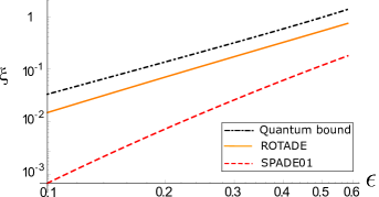
Figure 9: Chernoff exponent for Sinc PSF in function of the separation, with misalignment 0.25, $\sigma=1$.

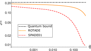
Figure 10: Chernoff exponent for Sinc PSF in function of the misalignment, for fixed separation 0.25, $\sigma=1$.

Similarly to the results in the main text, we verify in the limit asymptotic limit, ROTADE performs better than SPADE01.

Appendix C Performance of ROTADE in discrimination

Here we analyse the performance of ROTADE for the task of discriminating one and two light sources. As ROTADE involves only thee two-dimensional subspace spanned by the zeroth and first HG modes, an intrinsic error probability arises when the incoming radiation couples into higher HG modes. This probability is useful for defining the regime of validity of the qubit model.

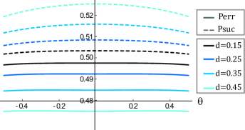
Figure 11: Error (solid) and success (dashed) probability in function of the reference position, using ROTADE for distinguishing between one and two sources, for different separations between the two sources.

For example Figure 11 presents the error and success probabilities in the regime where the centre of each distribution are aligned $\theta=0$. We observe that ROTADE has constant value (less than $4\%$ variation), e.g., at $\theta=0$ the error probability has value $P_{\mathrm{err}}=\frac{1}{2}\left(P_{\mathrm{err1}}+P_{\mathrm{err2}}\right)=\frac{1}{2}\left(0+e^{\frac{-d^{2}}{4\sigma^{2}}}\right)$, and the success probability $P_{\mathrm{suc}}=\frac{1}{2}\left(P_{\mathrm{suc1}}+P_{\mathrm{suc2}}\right)=\frac{1}{2}\left(1+\frac{d^{2}}{4\sigma^{2}}e^{\frac{-d^{2}}{4\sigma^{2}}}\right)$. As $d$ increases, the likelihood that photons couple to higher HG modes increases and hence the error (success) probability move further away from the priors, $0.5$. This is a consequence of the intrinsic error of the qubit model.

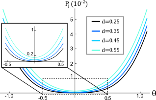
Figure 12: Intrinsic error of the qubit model ($\mathrm{P_{I}}$) in function of the misalignment $\theta$, for different separations $d$ between the sources.

The intrinsic error is the distance between the sum of the error and success probabilities from unity. It dictates until which separation and reference position the qubit model—and consequently ROTADE—are adequate. For $|\theta|<\frac{1}{2}$, or when the separation between the sources is comparable to $\sigma$, $\epsilon<\frac{1}{2}$, this error is negligible. This features are presented in Figure 12 and  13, respectively.

In Figure 12 we present the intrinsic error in function of the misalignment $\theta$. For a range of misalignments, $|\theta|<\frac{1}{2}$, ROTADE has negligible intrinsic error. Figure 13 shows the intrinsic error in function of the two source separation $\epsilon$, for misaligned source distributions, i.e., the centroid of the two sources is different from the center of one source ($x_{\mathrm{c}}\neq x_{0}$). We observe, that the qubit model is adequate when placing the measurement in between the distribution centroids $x_{\mathrm{c}}\leq x_{R}\leq x_{0}$ (in between red and orange lines) and the intrinsic error of the model is minimum when $\theta_{0}=\theta_{\mathrm{c}}$, i.e., when the centres of the two distributions coincide. Notice that when the centroids of the two distributions do not coincide the ROTADE measurement will, in general, depend on the separation of the two-source hypothesis.

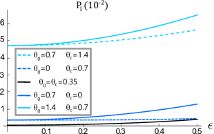
Figure 13: Intrinsic error of the qubit model ($\mathrm{P_{I}}$) in function of the separation $\epsilon$, for different values of the misalignment for the case where the center of one source is not equal with the two-source centroid ($\theta_{\mathrm{c}}\neq\theta_{0}$).

References

- Gisin and Thew (2007) N. Gisin and R. Thew, Nat. Photonics 1, 165 (2007).
- Smith (2010) G. Smith, in 2010 IEEE Information Theory Workshop (2010) pp. 1–5.
- Degen et al. (2017) C. L. Degen, F. Reinhard, and P. Cappellaro, Rev. Mod. Phys. 89, 035002 (2017).
- Pirandola et al. (2018) S. Pirandola, B. R. Bardhan, T. Gehring, C. Weedbrook, and S. Lloyd, Nat. Photonics 12, 724 (2018).
- Lemos et al. (2014) G. B. Lemos, V. Borish, G. D. Cole, S. Ramelow, R. Lapkiewicz, and A. Zeilinger, Nature 512, 409 (2014).
- Lloyd (2008) S. Lloyd, Science 321, 1463 (2008).
- Rayleigh (1879) L. Rayleigh, Lond.Edinb.Dubl.Phil.Mag. 8, 261 (1879).
- Acuna and Horowitz (2002) C. O. Acuna and J. Horowitz, J. Appl. Stat. 24, 421 (2002).
- Shahram and Milanfar (2004) M. Shahram and P. Milanfar, IEEE Trans. Image Process. 13, 677 (2004).
- Ram et al. (2006) S. Ram, E. S. Ward, and R. J. Ober, 103, 4457 (2006).
- Shahram and Milanfar (2006) M. Shahram and P. Milanfar, IEEE Trans. Inf. Theory 52, 3411 (2006).
- Tsang et al. (2016) M. Tsang, R. Nair, and X.-M. Lu, Phys. Rev. X 6, 031033 (2016).
- Svelto (1998) O. Svelto, Principles of lasers, 4th ed., Vol. 1 (Springer, 1998).
- Tsang (2020) M. Tsang, Contemp. Phys. 0, 1 (2020), publisher: Taylor & Francis _eprint: https://doi.org/10.1080/00107514.2020.1736375.
- Tsang (2017) M. Tsang, New J. Phys. 19, 023054 (2017).
- Tsang (2019) M. Tsang, Phys. Rev. A 99, 012305 (2019).
- Zhou and Jiang (2019) S. Zhou and L. Jiang, Phys. Rev. A 99, 013808 (2019).
- Bisketzi et al. (2019) E. Bisketzi, D. Branford, and A. Datta, New Journal of Physics 21, 123032 (2019).
- Sidhu and Kok (2017) J. S. Sidhu and P. Kok, Phys. Rev. A 95, 063829 (2017).
- Sidhu and Kok (2018) J. S. Sidhu and P. Kok, “Quantum fisher information for general spatial deformations of quantum emitters,” (2018), arXiv:1802.01601 [quant-ph] .
- Řehaček et al. (2017) J. Řehaček, Z. Hradil, B. Stoklasa, M. Paúr, J. Grover, A. Krzic, and L. L. Sánchez-Soto, Phys. Rev. A 96, 062107 (2017).
- Řeháček et al. (2018) J. Řeháček, Z. Hradil, D. Koutnỳ, J. Grover, A. Krzic, and L. L. Sánchez-Soto, Phys. Rev. A 98, 012103 (2018).
- Tsang and Nair (2019) M. Tsang and R. Nair, Optica 6, 400 (2019).
- Lupo and Pirandola (2016) C. Lupo and S. Pirandola, Phys. Rev. Lett. 117, 190802 (2016).
- Prasad and Yu (2019) S. Prasad and Z. Yu, Phys. Rev. A 99, 022116 (2019).
- Lu et al. (2018) X.-M. Lu, H. Krovi, R. Nair, S. Guha, and J. H. Shapiro, npj Quantum Inf. 4, 1 (2018).
- Len et al. (0) Y. L. Len, C. Datta, M. Parniak, and K. Banaszek, International Journal of Quantum Information 0, 1941015 (0), https://doi.org/10.1142/S0219749919410156 .
- Lupo (2020) C. Lupo, Phys. Rev. A 101, 022323 (2020).
- Gessner et al. (2020) M. Gessner, C. Fabre, and N. Treps, Phys. Rev. Lett. 125, 100501 (2020).
- Paúr et al. (2016) M. Paúr, B. Stoklasa, Z. Hradil, L. L. Sánchez-Soto, and J. Rehacek, Optica, OPTICA 3, 1144 (2016).
- Yang et al. (2016) F. Yang, A. Tashchilina, E. S. Moiseev, C. Simon, and A. I. Lvovsky, Optica 3, 1148 (2016).
- Tham et al. (2017) W.-K. Tham, H. Ferretti, and A. M. Steinberg, Phys. Rev. Lett. 118, 070801 (2017).
- Donohue et al. (2018) J. M. Donohue, V. Ansari, J. Řeháček, Z. Hradil, B. Stoklasa, M. Paúr, L. L. Sánchez-Soto, and C. Silberhorn, Phys. Rev. Lett. 121, 090501 (2018).
- Parniak et al. (2018) M. Parniak, S. Borówka, K. Boroszko, W. Wasilewski, K. Banaszek, and R. Demkowicz-Dobrzański, Phys. Rev. Lett. 121, 250503 (2018).
- Zhou et al. (2019) Y. Zhou, J. Yang, J. D. Hassett, S. M. H. Rafsanjani, M. Mirhosseini, A. N. Vamivakas, A. N. Jordan, Z. Shi, and R. W. Boyd, Optica, OPTICA 6, 534 (2019).
- Paúr et al. (2018) M. Paúr, B. Stoklasa, J. Grover, A. Krzic, L. L. Sánchez-Soto, Z. Hradil, and J. Řeháček, Optica, OPTICA 5, 1177 (2018).
- Grace et al. (2020) M. R. Grace, Z. Dutton, A. Ashok, and S. Guha, J. Opt. Soc. Am. A 37, 1288 (2020).
- Krovi et al. (2016) H. Krovi, S. Guha, and J. H. Shapiro, arXiv preprint arXiv:1609.00684 (2016).
- Morizur et al. (2010) J.-F. Morizur, L. Nicholls, P. Jian, S. Armstrong, N. Treps, B. Hage, M. Hsu, W. Bowen, J. Janousek, and H.-A. Bachor, J. Opt. Soc. Am. A 27, 2524 (2010).
- Wang et al. (2020) J. Wang, F. Sciarrino, A. Laing, and M. G. Thompson, Nature Photonics 14, 273 (2020).
- He et al. (2019) M. He, M. Xu, Y. Ren, J. Jian, Z. Ruan, Y. Xu, S. Gao, S. Sun, X. Wen, L. Zhou, et al., Nat. Photonics 13, 359 (2019).
- Chrostowski et al. (2017) A. Chrostowski, R. Demkowicz-Dobrzański, M. Jarzyna, and K. Banaszek, Int. J. Quantum Inf. 15, 1740005 (2017).
- Fowles (1989) G. R. Fowles, Introduction to modern optics (Dover Publications, INC., New York, 1989).
- Debes and Ge (2004) J. H. Debes and J. Ge, Publications of the Astronomical Society of the Pacific 116, 674 (2004).
- Yuen and Shapiro (1978) H. Yuen and J. H. Shapiro, IEEE Trans. Inf. Theory 24, 657 (1978).
- Kerviche et al. (2017) R. Kerviche, S. Guha, and A. Ashok, in 2017 IEEE International Symposium on Information Theory (ISIT) (IEEE, 2017) pp. 441–445.
- Rayleigh (1880) L. Rayleigh, Lond.Edinb.Dubl.Phil.Mag. 10, 116 (1880).
- Note (1) The results we mention also hold for multiple dimensions.
- Cramér (1961) H. Cramér, Mathematical Methods of Statistics (Princeton University Press, New Jersey, 1961).
- Fisher (1922) R. A. Fisher, Philos. Trans. R. Soc. A 222, 309 (1922).
- Wilks (1962) S. S. Wilks, Mathematical Statistics (John Wiley & Sons, New York, 1962).
- Helstrom (1976) C. W. Helstrom, Quantum Detection and Estimation Theory (Academic Press, 1976).
- Holevo (1982) A. S. Holevo, Probabilistic and Statistical Aspects of Quantum Theory (North Holland, 1982).
- Ragy et al. (2016) S. Ragy, M. Jarzyna, and R. Demkowicz-Dobrzański, Phys. Rev. A 94, 052108 (2016).
- Demkowicz-Dobrzański et al. (2020) R. Demkowicz-Dobrzański, W. Górecki, and M. Guţă, Journal of Physics A: Mathematical and Theoretical 53, 363001 (2020).
- Albarelli et al. (2020) F. Albarelli, M. Barbieri, M. Genoni, and I. Gianani, Physics Letters A 384, 126311 (2020).
- Hong et al. (1987) C. K. Hong, Z. Y. Ou, and L. Mandel, Phys. Rev. Lett. 59, 2044 (1987).
- Note (2) The case of continuous random variables follows similarly.
- Rényi (1966) A. Rényi, in Research Papers in Statistics: Festschrift for J. Neyman(F. N. David, ed.), (New York) , 281 (1966).
- Neyman and Pearson (1933) J. Neyman and E. S. Pearson, IX. Philosophical Transactions of the Royal Society of London. Series A, Containing Papers of a Mathematical or Physical Character 231, 289 (1933).
- Chernoff (1952) H. Chernoff, Ann. Math. Statist. 23, 493 (1952).
- Audenaert et al. (2007) K. M. R. Audenaert, J. Calsamiglia, R. Muñoz Tapia, E. Bagan, L. Masanes, A. Acin, and F. Verstraete, Phys. Rev. Lett. 98, 160501 (2007).
- Nussbaum and Szkoła (2009) M. Nussbaum and A. Szkoła, The Annals of Statistics 37, 1040 (2009).
- Helstrom (1973) C. Helstrom, IEEE Transactions on Information Theory 19, 389 (1973).