Constraints on charm-anticharm asymmetry in the nucleon from lattice QCD
Abstract
We present the first lattice QCD calculation of the charm quark contribution to the nucleon electromagnetic form factors in the momentum transfer range . The quark mass dependence, finite lattice spacing and volume corrections are taken into account simultaneously based on the calculation on three gauge ensembles including one at the physical pion mass. The nonzero value of the charm magnetic moment , as well as the Pauli form factor, reflects a nontrivial role of the charm sea in the nucleon spin structure. The nonzero indicates the existence of a nonvanishing asymmetric charm-anticharm sea in the nucleon. Performing a nonperturbative analysis based on holographic QCD and the generalized Veneziano model, we study the constraints on the distribution from the lattice QCD results presented here. Our results provide complementary information and motivation for more detailed studies of physical observables that are sensitive to intrinsic charm and for future global analyses of parton distributions including asymmetric charm-anticharm distribution.
keywords:
Intrinsic charm , Form factor , Parton distributions , Lattice QCD, Light-front holographic QCD , JLAB-THY-20-3155, SLAC-PUB-175151 Introduction
The charm-anticharm sea in the nucleon has received great interest in nuclear and particle physics for its particular significance in understanding high energy reactions associated with charm production. Quantum Chromodynamics (QCD), the underlying theory of the strong interaction, allows heavy quarks in the nucleon-sea to have both perturbative “extrinsic” and nonperturbative “intrinsic” origins. The extrinsic sea arises from gluon splitting triggered by a probe in the reaction. It can be calculated order-by-order in perturbation theory if the probe is hard. The intrinsic sea is encoded in the nucleon wave functions.
The existence of nonperturbative intrinsic charm (IC) was originally proposed in the BHPS model [1] and in the subsequent calculations [2, 3, 4] following the original proposal [1]. Proper knowledge of the existence of IC and an estimate of its magnitude will elucidate some fundamental aspects of nonperturbative QCD. Therefore, the main goal of this article is to investigate the existence of nonzero “intrinsic” charm of nonperturbative origin in the nucleon. In the case of light-front (LF) Hamiltonian theory, the intrinsic heavy quarks of the proton are associated with higher Fock states such as in the hadronic eigenstate of the LF Hamiltonian; this implies that the heavy quarks are multi-connected to the valence quarks. The probability for the heavy-quark Fock states scales as in non-Abelian QCD. Since the LF wavefunction is maximal at minimum off-shell invariant mass; i.e., at equal rapidity, the intrinsic heavy quarks carry large momentum fraction . A key characteristic is different momentum and spin distributions for the intrinsic and in the nucleon, as manifested, for example, in charm-anticharm asymmetry [5, 6], since the comoving quarks can react differently to the global quantum numbers of the nucleon [7].
IC was also proposed in meson-baryon fluctuation models [8, 9]. The possible direct and indirect relevance of IC in several physical processes has led to many phenomenological calculations involving the existence of a non-zero IC to explain anomalies in the experimental data and possible signatures of IC in upcoming experiments [7]. Unfortunately, the normalization of the intrinsic charm Fock component in the light-front wavefunctions (LFWF) is unknown. Also, the probability to find a two-body state in the proton within the meson-baryon fluctuation models cannot be determined without additional assumptions: precise constraints from future experiments and/or first-principles calculations are required.
The effect of whether the IC parton distribution is either included or excluded in the determinations of charm parton distribution functions (PDFs) can induce changes in other parton distributions through the momentum sum rule, which can indirectly affect the analyses of various physical processes that depend on the input of various PDFs. An estimate of intrinsic charm () and anticharm () distributions can provide important information to the understanding of charm quark production in the EMC experiment [10]. The enhancement of charm distribution in the measurement of the charm quark structure function compared to the expectation from the gluon splitting mechanism in the EMC experimental data has been interpreted as evidence for nonzero IC in several calculations [2, 3, 11, 12]. A precise determination of and PDFs by considering both the perturbative and nonperturbative contributions is important in understanding charmonia and open charm productions, such as the production at large momentum from collisions at CERN [13], from collisions at FNAL [14], from collisions at LHC [15], and charmed hadron or jet production from collisions at ISR, FNAL, and LHC [15, 16, 17, 18]. LHC measurements associated with cross section of inclusive production of Higgs, , bosons via gluon-gluon fusion, and productions of charm jet and [19, 20, 21, 22], and mesons at LHCb experiment [15] can also be sensitive to the IC distribution. The photo- or electro-productions near the charm threshold is believed to be sensitive to the trace anomaly component of the proton mass, and some experiments have been proposed at JLab [23] as well as for the future EIC to measure the production cross section near the threshold. The existence of IC in the proton will provide additional production channels and thus enhance the cross section, especially near the threshold. Similarly, open charm production will also be enhanced by IC. If and quarks have different distributions in the proton, the enhancements on and productions will appear at slightly different kinematics. IC has also been proposed to have an impact on estimating the astrophysical neutrino flux observed at the IceCube experiment [24].
In global analyses of PDFs there are different approaches to deal with heavy quarks in which a transition of the number of active quark flavors is made at some scale around the charm quark mass [25, 26, 27, 28]. The transition scale defines where the extrinsic charm-anticharm sea enters. However, the intrinsic charm-anticharm sea can exist even at a lower scale. In many global fits [29, 30, 31, 32, 33, 34], the charm quark PDF is set to zero at , but this is an assumption of no IC. In recent years, several PDF analyses started to investigate the possibility of nonzero charm and anticharm distributions at the scale [35, 36, 37, 38, 39], but none of them can provide conclusive evidence or exclusion for the intrinsic charm due to the absence of precise data. A nonzero charm quark PDF at is not necessarily evidence of intrinsic charm, because such estimation depends on the heavy-quark scheme and the value used in the fit. This explains the speculation in [35] that the estimation of intrinsic charm may strongly depend on the choice of the transition scale . Fortunately, there is an ideal quantity, the asymmetric charm-anticharm distribution , which would be a clear signal for IC. Such asymmetry is allowed in QCD because the nucleon has nonzero quark number, the number of quarks minus the number of antiquarks, and thus the quark and the quark in a nucleon would “feel” different interactions, leading to an asymmetric charm-anticharm distribution. Although the absence of such asymmetry does not exclude intrinsic charm, a nonzero can serve as strong evidence, because the extrinsic part of such asymmetry arising at the next-to-next-to-leading order level is negligible [40].
Although the global fits [35, 36, 37, 38, 39] consider the possibility of IC, all these fits assume ; constraints on have been warranted in the global fit [38]. It was found in [38] that a precise and accurate parametrization of the charm PDFs will be useful for more reliable phenomenology using the data from LHC experiments and will eliminate possible sources of bias arising from the assumptions of only perturbatively-generated charm PDFs. It is therefore important to determine if , and how or whether the IC will have significant effect in the physical processes [13, 14, 15, 16, 17, 18, 19, 20, 21, 22]. A precise and accurate knowledge of the IC will also have a direct impact on determining the unknown normalization constants of different model calculations associated with the nonperturbative and distributions.
An important question to ask is whether the first-principles lattice QCD (LQCD) calculation can provide some constraints or complementary information regarding the existence of IC. Recently, there have been LQCD calculations of the strange quark electromagnetic form factors [41, 42, 43, 44, 45, 46] with higher precision and accuracy than previously attained by experiments. These LQCD calculations provided indirect evidence for a nonzero strange quark-antiquark asymmetry in the nucleon by pinning down the nonzero value of the strange electric form factor at . The determination of from the LQCD calculation in [42] has led to precise determination of neutral current weak axial and electromagnetic form factors [44, 47]. Using LQCD results from [42, 43] as constraints, it has been shown recently in [48], within the light-front holographic QCD (LFHQCD) approach [49, 50, 51, 52] and the generalized Veneziano model [53, 54, 55], that the distribution is negative at small- and positive at large-. This shows the possibility of applying LQCD results for the phenomenological study of the asymmetry in the absence of precise experimental data and global fits of the strange quark PDFs.
The main goal of this article is to calculate the charm electric and magnetic form factors, and , from LQCD at nonzero momentum transfer and discuss their connection to the existence of IC and a nonzero asymmetry distribution in the nucleon. Using the LQCD calculation of as constraint, we determine the distribution using the nonperturbative framework described in [56]. We note that the electromagnetic current is odd under charge conjugation and the Dirac form factor provides a measure of the -quark minus the -quark contribution due to the opposite charges of the quark and antiquark. While , required by the quantum numbers of the nucleon, a positive at implies that the -quark distribution is more centralized than the quark distribution in coordinate space. This, in turn, results in a asymmetry in momentum space, thereby providing possible evidence for the nonperturbative IC in the nucleon. On the other hand, a nonzero charm Pauli form factor and a nonzero charm magnetic moment are consequences of a nonzero orbital angular momentum contribution to the nucleon from charm quarks [57]. This can be understood in the inherently relativistic LF formalism where a nonzero anomalous magnetic moment requires to have orbital angular momentum and Fock-states components in the LFWF.
The remainder of this article is organized as follows: In Section 2, we briefly discuss the LQCD calculation of the charm electromagnetic form factors and determine these in the physical limit. In Section 3, we use LQCD results for as input for quantitative analysis of the asymmetry distribution in the nucleon within the specific framework of LFHQCD and the generalized Veneziano model. We also present a brief qualitative discussion of our results in Section 4.
2 Lattice QCD calculation of
We present in this section the first lattice QCD calculation of the charm quark electromagnetic form factors in the nucleon. This first-principles analysis requires a disconnected insertion calculation. By “disconnected insertion,” one refers to the nucleon matrix elements involving self-contracted quark graphs (loops), which are correlated with the valence quarks in the nucleon propagator by the fluctuating background gauge fields. (Notice the distinction with the term “disconnected diagram” used in the continuum Quantum Field Theory literature.) Numerical expense and complexity of the disconnected insertion calculations in LQCD, the deficit of good signal-to-noise ratio in the matrix elements, and the possibility for a very small magnitude of the quark matrix elements make it difficult to obtain a precise determination of . We, therefore, need to accept several limitations while performing this calculation. For example, the data is almost twice as noisy compared to the matrix elements of the strange electromagnetic form factors [42, 43, 44] and we do not see any signal for one of the gauge ensembles (32ID with a lattice spacing of fm [58]) used in the previous calculations [42, 44]. Moreover, we are only able to perform the widely used two-states summed ratio fit of the nucleon three-point () to two-point () correlation functions instead of a simultaneous fit to the summed ratio and conventional -ratio as was done in [44]. The reason is that the -ratio fit for extracting is not stable for the ensemble at the physical pion mass MeV. We also keep in mind that the errors associated with the lattice spacing can be larger than the case for the matrix elements.
Our calculation comprises numerical computation with valence overlap fermion on three RBC/UKQCD domain-wall fermion gauge configurations [58, 59]: (ensemble ID, , , , , )={(48I, , 2.13, 0.1141(2), 139, 81), (32I, , 2.35, 0.0828(3), 300, 309), (24I, , 2.13, 0.1105(3), 330, 203)}. Here is spatial and is temporal size, is lattice spacing, is the pion mass corresponding to the degenerate light-sea quark mass and is the number of configurations. We use 17 valence quark masses across these ensembles to explore the quark-mass dependence of the charm electromagnetic form factors. The details of the numerical setup of this calculation can be found in [60, 61, 62, 44]. was determined in a global fit on the lattice ensembles with fm and using inputs from three physical quantities, such as , , and in [63]. Our statistics are from approximately 100k to 500k measurements across the 24I to 48I ensembles. The quark loop is calculated with the exact low eigenmodes (low-mode average) while the high modes are estimated with 8 sets of noise [64] on the same grid with odd-even dilution and additional dilution in time. We refer the readers to previous work [44] for a detailed discussion of the similar numerical techniques which have been used for this calculation.

can be obtained by the ratio of a combination of 3pt and 2pt correlations as,
| (1) | |||||
Here, is the nucleon 2pt function, is the nucleon 3pt function with the bilinear operator , and is the nucleon mass, is the three-momentum transfer with sink momentum and the source momentum . The projection operator for is and that for is with . contains a ratio , where is the wavefunction overlap for the point sink with momentum . As estimated in [44], the error introduced by neglecting this factor is about compared to the statistical error in the matrix elements and thus it is ignored in this work. We extract matrix elements using the two-states fit of the nucleon summed ratio for a given and fixed index in Eq. (1):
| (2) |
Here, is the -ratio, and are the source and sink temporal positions, respectively, and is the time at which the bilinear operator is inserted, and are the number of time slices we drop at the source and sink sides, respectively, and we choose . are the spectral weights involving the excited-state contamination. Ideally, is the energy difference between the first excited state and the ground state but in practice, this is an average of the mass difference between the proton and the lowest few excited states. As shown in [44], the -ratio data points are almost symmetric between the source and sink within uncertainty and introducing two does not change the fit results of . The excited states in the fit fall off faster as compared to the two-states fit case of the -ratio where the excited-state falls off at a slower rate as . These faster-decreasing excited-state effects allow for fitting the matrix elements starting from shorter time extents, as was demonstrated in [65]. In Fig. 1, we present a sample extraction of matrix elements on 48I at MeV pion mass at GeV2 which enables us to demonstrate the extraction of with signal-to-noise ratio better than at other data points on the 48I ensemble. We also present a similar example on the 32I ensemble at MeV and at the largest where the excited-state contribution is expected to be the largest. For example, we obtain , on the 48I ensemble and , on the 32I ensemble in the fits.
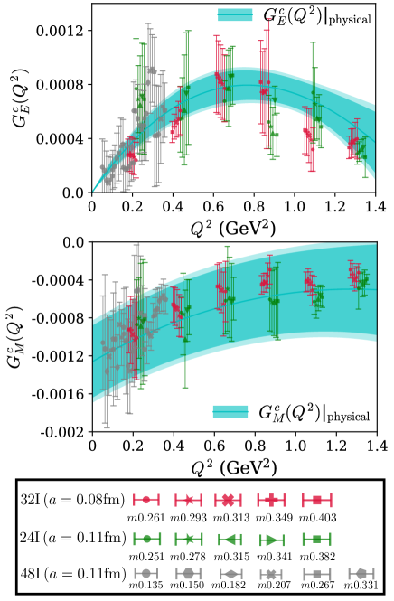
We present the matrix elements of obtained from the fit Eq. (2) in the upper and lower panels of Fig. 2. With the extracted 102 matrix elements from three gauge ensembles (for each of and ) at different pion masses and , we perform a simultaneous correlated and model-independent -expansion fit [66, 67] to in the momentum transfer range of GeV2 and perform chiral, continuum (lattice spacing ), and infinite volume limit (lattice spatial extent ) extrapolations to obtain the form factors in the physical limit. For such a fit to , we adopt the following fit form
| (3) |
| (4) |
In fit Eq. (2), is the partially quenched pion mass with the pion mass corresponding to the sea quark mass. The masses for the lattice ensembles are obtained in [63] and extrapolated to the physical value GeV [68]. includes the mixed-action parameter [69]. The volume correction in fit (2) has been adopted from [70] to best describe the data. We use , the pole of pair production. We note that this choice is different from the fit to the strange quark form factor where the is chosen at , because the mass of two kaons is less than the mass of , while the mass of two mesons is greater than the mass of . One may also consider , which is a bit lighter, but is more likely to be produced from a vector current.
The inclusion of higher-order terms beyond has no statistical significance and is not considered in the -expansion fit (2). We obtain for the fit (2) and the fit parameters are , , , , , , , , , . Replacing the correction term by results in negligible change in the final result. A faster decreasing volume correction correction gives which is a smaller correction compared to as expected and they are in statistical agreement. The significant increase of the uncertainty in the physical value of at larger is due to the fact that the data points on the 24I and 32I ensembles are at much heavier pion mass compared to the matrix element at the physical MeV on the 48I ensemble and there exist no LQCD data points at GeV2 on the 48I ensemble. We also see a similar feature for shown in the lower panel of Fig. 2. The cyan band in Fig. 2 represents in the physical limit after the quark mass, finite lattice spacing and volume corrections have been implemented using the fit parameters listed above. Since most of the corrections do not have statistical significance, we explore the above fit with separate combinations of , for example, with , , and correction terms. For these fits, we obtain , , and , while the physical remains essentially unchanged with slightly smaller final uncertainties compared to when all corrections are included. A similar investigation for the fit results in a similar conclusion.
The systematic uncertainty is estimated by calculating the differences between and obtained from the fit Eq. (2) by considering the corrections of the , , terms from the -value on the 24I ensemble obtained in [63], the smallest lattice spacing from the 32I ensemble, and the 48I ensemble with the largest volume, respectively. The systematic uncertainty has been added as lighter-tinted margins to the statistical uncertainty band in Fig. 2.
To obtain in the physical limit and in the GeV2 momentum transfer region, we adopt the following empirical fit form with the volume correction term adopted from [71]:
| (5) |
We limit the in our fit. Additional terms in the -expansion have no statistically significant effect on . With the in the fit (2), we obtain the fit parameters , , , , , , , , and . The systematic uncertainty of is obtained in a similar way as for the case of .
The electric and magnetic radii can be extracted from the slope of the form factors as :
| (6) |
Using the -values from above, we obtain
| (7) |
While the existence of a nonzero (and thus the Dirac form factor) is related to a nonzero asymmetry of the distribution, a nonzero (and thus Pauli form factor) immediately implies that there is a nonzero orbital angular momentum contribution to the nucleon from the charm quarks. The Pauli form factor has the LFWF representation as the overlap of the states differing by one unit of orbital angular momentum. It is thus closely related to the spin sector of the charm quark sea in the proton. is also given by the first moment of the generalized parton distribution , , which contributes to the second term of Ji’s sum rule [72]. Therefore, our result indicates a nontrivial role of the charm quark sea in understanding the spin content of the proton.
3 A nonperturbative model for computing the intrinsic ] asymmetry in the nucleon
Although a model-independent determination of IC distributions from the charm quark form factors is not possible at the moment, the underlying physics, governed by QCD, does imply some important connections and constraints, such as the QCD inclusive-exclusive connection [73, 74, 75]: It relates hadron form factors at large to the hadron structure function at , leading to simple counting rules. Furthermore, since the and carry opposite charges, the charm quark form factor measures the difference of the transverse charge density [76] between the and quarks. For a positive charge form factor, like those shown in Fig. 2, the charm quark distribution is more spread out than the anticharm distribution in -space, where is the Fourier conjugate variable of the transverse coordinate and . As a feature of Fourier transform, the charm quark density is more centralized in -space than the anticharm quark. Representing the density as the square of the wave function, , one can easily find the -space wave function is more spread out for the charm quark, where is the intrinsic transverse momentum. Thus the actual distribution for a positive charge form factor favors the quark carrying higher momentum than the quark. As a result, the distribution will favor negative values in the low- region and positive values in the high- region. We note that a strict definition of the transverse charge density is given by the Fourier transform of the Dirac form factor , which dominates the charge form factor in the low- regime.
For a quantitative estimation of , one currently has to rely on additional assumptions, although the form factor result does indicate some qualitative features of the distribution function based on the discussions above. Here we take the nonperturbative phenomenological model in [48], which relates the form factor and sea-quark distribution functions with minimal parameters. The formalism is based on the gauge/gravity correspondence [77], light-front holographic mapping [51, 52, 56], and the generalized Veneziano model [53, 54, 55]. In the following, we refer to this model as LFHQCD. The charm quark Dirac and Pauli form factors are given by [78]
| (8) | |||||
| (9) |
where is the number of constituents of the Fock state component. The leading Fock state with nontrivial contribution to the charm form factor is , which is a state. With additional intrinsic sea quark pairs, the Fock states, e.g. , , etc., will contribute to terms. If also considering the possibility of intrinsic gluon constituents, one may have the contribution from , , and/or higher Fock states.
Form factor can be expressed in a reparametrization invariant form [56]
| (10) |
where is the Regge trajectory, and is a normalization factor; is a flavor independent function with and . We use the same universal form of the function from [56]
| (11) |
with [83]: It incorporates Regge behavior at small with the intercept (14), as , and the inclusive-exclusive counting rule at large , , as [56]. The light front holographic approach leading to these results is based on the underlying conformal algebra which leads to linear Regge trajectories. The spin-flavor coefficients and are parameters to be determined from the LQCD computation of and to obtain . The constraint that the numbers of charm and anticharm quarks are identical for each Fock state component has been incorporated in Eq. (8).
Then the asymmetric charm-anticharm distribution function is
| (12) |
where and
| (13) |
We should note here that the coefficients in Eq. (12) are the same as those in Eq. (8). Therefore, once they are determined by the form factor, one can make predictions for the distribution functions.
The form factors and distribution functions above are derived at the massless quark limit and one may have different approaches to incorporate quark mass corrections. For small quark masses (up, down and strange) the latter can be treated perturbatively, leaving the Regge slope unchanged and leading to a moderate change of the intercept. The resulting spectra are in very good agreement with experiment [51, 79]. The situation is more intricate for the case of heavy quarks, like quarks, since now conformal symmetry is strongly broken and the occurrence of linear trajectories is far from obvious. It has been shown, however, that the formalism can indeed be extended to heavy quark bound states [80, 81], leading to a fair agreement with the data. In this case, the Regge trajectories are still linear, but the slope depends on the heavy quark mass. The intercept changes quite drastically with the quark mass.
The Regge trajectory obtained in [81] is
| (14) |
where . This result agrees with the one obtained in a phenomenological potential model [82]. The large change of the intercept as compared to light quarks removes the small- singularity of quark distribution functions while keeping the counting rules at large and at large unchanged. The change of the slope affects only the generalized parton distribution function. The quark distribution difference is not sensitive to the choice of the mass correction procedure, since the quark mass affects equally charm and anticharm distributions.
In practice, one needs to truncate the expansion in Eq. (8) to have numerical results. For simplicity, we only keep the lowest Fock state containing the charm quark components, i.e., . The coefficient is determined, through Eqs. (8) and (9) by the lattice results of and at the physical limit. We perform a fit to the extracted results of and , i.e., the bands in Figs. 2. Since the lattice data from different ensembles are evaluated at different values, and have been utilized to determine the quark mass, lattice spacing, and finite volume effects, the effective number of data points in the physical limit is 6 for and 6 for 111For each ensemble we have data points at 6 different . A simultaneous fit of the data from three ensembles (48I, 32I, 24I) with different quark masses, lattice spacings, and volumes leads to the results in the physical limit.. To really capture the uncertainty, we create 200 replicas from the extracted bands. Each replica is firstly generated by randomly sampling 6 data points of and 6 data points of from the extracted bands within , which are covered by the lattice data. Then for each data point, the central value is resampled with a Gaussian distribution according to its uncertainty. In addition, we also randomly shift the value of within in each single fit of one replica to incorporate the theoretical uncertainty. The coefficient determined from the fit is .
Having obtained the charm coefficient from the lattice computation, we use Eq. (12), to obtain the asymmetric charm-anticharm distribution function shown in Fig. 3. The result from the fit is in agreement with the qualitative analysis at the beginning of this section, namely, that the charm quark tends to carry larger momentum than the anticharm quark based on the lattice results for the charm quark form factors.

From the distribution obtained by combining LQCD results from and the LFHQCD formalism, we can calculate the first moment of the difference of and PDFs to be
| (15) |
where the total uncertainty is obtained from the fitting error in and 5% variation in . The distribution result is about 3 times smaller in magnitude than the distribution obtained with the same formalism [48]. Although a small asymmetry could be a result of the cancellation of two relatively large and distributions, it is possible that the intrinsic charm and anticharm distributions are both small. Furthermore, the charm and anticharm distributions at high energy scales are dominated by the extrinsic sea from perturbative radiation. The experimental observation and isolation of the intrinsic charm effect are extremely challenging in such cases. Thus it is not surprising that the recent measurement of and productions by the LHCb collaboration [15] found no intrinsic charm effect. An ideal place to investigate intrinsic charm would be the or open charm productions at relatively low energies, e.g., at JLab, although it is also possible to see intrinsic charm effects in very accurate measurements of high energy reactions. In addition, lepton-nucleon scattering may provide a cleaner probe than nucleon-nucleon scattering to help reduce backgrounds and increase the chance to observe the intrinsic charm effect, and therefore the future EIC will provide such opportunities.
The nonzero value of can also originate from the interference of the and sub-processes, without the existence of IC. However, as mentioned earlier, this extrinsic asymmetry which arises at the next-to-next-to-leading order level is negligible [40]. Moreover, according to [40], this extrinsic asymmetry would result in a much smaller and negative value of the first moment of distribution compared to obtained in this calculation. A negative value for would also result in a positive distribution at small and a negative distribution at large , in contrast to the distribution we have obtained here. But the evidence based on the distribution in [48], the EMC measurement [10], and perturbative QCD computation [40] seem to indicate extremely small values of extrinsic charm for . The present determination of the distribution from LQCD supports the existence of nonperturbative intrinsic heavy quarks in the nucleon wavefunction at large with a magnitude consistent with experimental signals. A consequence of this result is Higgs production at large in collisions at the LHC from the direct coupling of the Higgs to the intrinsic heavy quark pair [84].
4 Conclusion and outlook
In this article, we have presented the first lattice QCD calculation of the charm quark electromagnetic form factors in the physical limit. This first lattice QCD calculation indicates that a nonzero charm electric form factor corresponds to the intrinsic charm-anticharm asymmetry in the nucleon sea, thereby providing an indication of the existence of nonzero intrinsic charm based on a first-principles calculation. In addition, the nonzero value of the charm magnetic form factor indicates a nonzero orbital angular momentum contribution to the nucleon coming from the charm quarks. We have discussed that the existence of IC is supported by QCD and how an accurate knowledge of the intrinsic charm can help to remove bias in the global fits of PDFs and related phenomenological studies.
Motivated by the new lattice results, we have used the nonperturbative light-front holographic framework incorporating the QCD inclusive-exclusive connection at large to determine the asymmetry up to a normalization factor, which is constrained by the lattice QCD calculation. Since the LFHQCD calculation starts from a nucleon Fock state with hidden charm, the parton distributions determined in this model refer exclusively to intrinsic charm where the small- behavior is determined by the intercept. On the other hand, contributions from gluon splitting are supposed to be determined by the pomeron trajectory with a much higher intercept. These features will be discussed in a separate publication.
The new determination of the asymmetry presented here gives additional elements and further insights into the existence of intrinsic charm. It also can provide complementary information to the global fits of PDFs which look for the possibility of IC in the absence of ample experimental data.
Acknowledgements
RSS thanks Jeremy R. Green, Luka Leskovec, Jian-Wei Qiu, Anatoly V. Radyushkin, and David G. Richards for useful discussions. The authors thank the RBC/UKQCD collaborations for providing their DWF gauge configurations. This work is supported by the U.S. Department of Energy, Office of Science, Office of Nuclear Physics under contract DE-AC05-06OR23177. A. Alexandru is supported in part by U.S. DOE Award Number DE-FG02-95ER40907. T. Draper and K.F. Liu are supported in part by DOE Award Number DE-SC0013065. Y. Yang is supported by Strategic Priority Research Program of Chinese Academy of Sciences, Grant No. XDC01040100. This research used resources of the Oak Ridge Leadership Computing Facility at the Oak Ridge National Laboratory, which is supported by the Office of Science of the U.S. Department of Energy under Contract No. DE-AC05-00OR22725. This work used Stampede time under the Extreme Science and Engineering Discovery Environment (XSEDE), which is supported by National Science Foundation grant number ACI-1053575. We also thank the National Energy Research Scientific Computing Center (NERSC) for providing HPC resources that have contributed to the research results reported within this paper. We acknowledge the facilities of the USQCD Collaboration used for this research in part, which are funded by the Office of Science of the U.S. Department of Energy.
References
- [1] S. J. Brodsky, P. Hoyer, C. Peterson, and N. Sakai, “The intrinsic charm of the proton,” Phys. Lett. 93B, 451 (1980).
- [2] S. J. Brodsky, J. C. Collins, S. D. Ellis, J. F. Gunion, and A. H. Mueller, “Intrinsic Chevrolets at the SSC,” in Proceedings of the 1984 Summer Study on the SSC, Snowmass, CO, edited by R. Donaldson and J. G. Morfin (AIP, New York, 1985).
- [3] B. W. Harris, J. Smith and R. Vogt, “Reanalysis of the EMC charm production data with extrinsic and intrinsic charm at NLO,” Nucl. Phys. B 461, 181 (1996).
- [4] M. Franz, M. V. Polyakov, and K. Goeke, “Heavy quark mass expansion and intrinsic charm in light hadrons,” Phys. Rev. D 62, 074024 (2000).
- [5] S. J. Brodsky and B. Q. Ma, “The quark-antiquark asymmetry of the nucleon sea,” Phys. Lett. B 381, 317 (1996).
- [6] W. Melnitchouk and A. W. Thomas, “HERA anomaly and hard charm in the nucleon,” Phys. Lett. B 414, 134 (1997).
- [7] S. J. Brodsky, A. Kusina, F. Lyonnet, I. Schienbein, H. Spiesberger and R. Vogt, “A review of the intrinsic heavy quark content of the nucleon,” Adv. High Energy Phys. 2015, 231547 (2015).
- [8] F. S. Navarra, M. Nielsen, C. A. A. Nunes and M. Teixeira, “On the intrinsic charm component of the nucleon,” Phys. Rev. D 54, 842 (1996).
- [9] J. Pumplin, “Light-cone models for intrinsic charm and bottom,” Phys. Rev. D 73, 114015 (2006).
- [10] J. J. Aubert et al. [European Muon Collaboration], “Production of charmed particles in 250-GeV - iron interactions,” Nucl. Phys. B 213, 31 (1983).
- [11] E. Hoffmann and R. Moore, “Subleading contributions to the intrinsic charm of the nucleon,” Z. Phys. C 20, 71 (1983).
- [12] S. J. Brodsky, P. Hoyer, A. H. Mueller and W. K. Tang, “New QCD production mechanisms for hard processes at large ,” Nucl. Phys. B 369, 519 (1992).
- [13] J. Badier et al. [NA3 Collaboration], “Experimental hadronic production from 150 to 280 GeV/c,” Z. Phys. C 20, 101 (1983).
- [14] M. J. Leitch et al. [NuSea Collaboration], “Measurement of and suppression in collisions,” Phys. Rev. Lett. 84, 3256 (2000).
- [15] R. Aaij et al. [LHCb Collaboration], “First measurement of charm production in its fixed-target configuration at the LHC,” Phys. Rev. Lett. 122, 132002 (2019).
- [16] P. Chauvat et al. [R608 Collaboration], “Production of with large at the ISR,” Phys. Lett. B 199, 304 (1987).
- [17] E. M. Aitala et al. [E791 Collaboration], “Asymmetries in the production of and baryons in 500 GeV/c nucleon interactions,” Phys. Lett. B 495, 42 (2000).
- [18] E. M. Aitala et al. [Fermilab E791 Collaboration], “Differential cross sections, charge production asymmetry, and spin-density matrix elements for (2010) produced in 500-GeV/c -nucleon interactions,” Phys. Lett. B 539, 218 (2002).
- [19] G. Aad et al. [ATLAS Collaboration], “Measurement of and -boson production cross sections in collisions at TeV with the ATLAS detector,” Phys. Lett. B 759, 601 (2016).
- [20] G. Aad et al. [ATLAS Collaboration], “Measurement of the boson transverse momentum distribution in collisions at = 7 TeV with the ATLAS detector,” JHEP 1409, 145 (2014).
- [21] G. Aad et al. [ATLAS Collaboration], “Measurement of the transverse momentum and distributions of Drell-Yan lepton pairs in proton-proton collisions at TeV with the ATLAS detector,” Eur. Phys. J. C 76, 291 (2016).
- [22] V. Khachatryan et al. [CMS Collaboration], “Measurement of the Z boson differential cross section in transverse momentum and rapidity in proton-proton collisions at 8 TeV,” Phys. Lett. B 749, 187 (2015).
- [23] Jefferson Lab experiment E12-12-006, Near Threshold Electroproduction of at 11 GeV, spokespersons: K. Hafidi, Z.-E. Meziani, X. Qian, N. Sparveris, Z. W. Zhao.
- [24] R. Laha and S. J. Brodsky, “IceCube can constrain the intrinsic charm of the proton,” Phys. Rev. D 96, 123002 (2017).
- [25] M. A. G. Aivazis, J. C. Collins, F. I. Olness and W. K. Tung, “Leptoproduction of heavy quarks. 2. A unified QCD formulation of charged and neutral current processes from fixed-target to collider energies,” Phys. Rev. D 50, 3102 (1994).
- [26] M. Buza, Y. Matiounine, J. Smith and W. L. van Neerven, “Charm electroproduction viewed in the variable-flavor number scheme versus fixed-order perturbation theory,” Eur. Phys. J. C 1, 301 (1998).
- [27] S. Forte, E. Laenen, P. Nason and J. Rojo, “Heavy quarks in deep-inelastic scattering,” Nucl. Phys. B 834, 116 (2010).
- [28] R. S. Thorne, “Effect of changes of variable flavor number scheme on parton distribution functions and predicted cross sections,” Phys. Rev. D 86, 074017 (2012).
- [29] S. Alekhin, J. Blumlein and S. Moch, “The ABM parton distributions tuned to LHC data,” Phys. Rev. D 89, 054028 (2014).
- [30] L. A. Harland-Lang, A. D. Martin, P. Motylinski and R. S. Thorne, “Parton distributions in the LHC era: MMHT 2014 PDFs,” Eur. Phys. J. C 75, 204 (2015).
- [31] R. D. Ball et al. [NNPDF Collaboration], “Parton distributions for the LHC Run II,” JHEP 1504, 040 (2015).
- [32] S. Dulat et al., “New parton distribution functions from a global analysis of quantum chromodynamics,” Phys. Rev. D 93, 033006 (2016).
- [33] H. Abramowicz et al. [H1 and ZEUS Collaborations], “Combination of measurements of inclusive deep inelastic scattering cross sections and QCD analysis of HERA data,” Eur. Phys. J. C 75, 580 (2015).
- [34] A. Accardi, L. T. Brady, W. Melnitchouk, J. F. Owens and N. Sato, “Constraints on large- parton distributions from new weak boson production and deep-inelastic scattering data,” Phys. Rev. D 93, 114017 (2016).
- [35] S. Dulat, T. J. Hou, J. Gao, J. Huston, J. Pumplin, C. Schmidt, D. Stump and C.-P. Yuan, “Intrinsic charm parton distribution functions from CTEQ-TEA global nalysis,” Phys. Rev. D 89, 073004 (2014).
- [36] J. Pumplin, H. L. Lai and W. K. Tung, “Charm parton content of the nucleon,” Phys. Rev. D 75, 054029 (2007).
- [37] P. Jimenez-Delgado, T. J. Hobbs, J. T. Londergan and W. Melnitchouk, “New limits on intrinsic charm in the nucleon from global analysis of parton distributions,” Phys. Rev. Lett. 114, 082002 (2015).
- [38] R. D. Ball et al. [NNPDF Collaboration], “A determination of the charm content of the proton,” Eur. Phys. J. C 76, 647 (2016).
- [39] T. J. Hou et al., “CT14 intrinsic charm parton distribution functions from CTEQ-TEA global analysis,” JHEP 1802, 059 (2018).
- [40] S. Catani, D. de Florian, G. Rodrigo and W. Vogelsang, “Perturbative generation of a strange-quark asymmetry in the nucleon,” Phys. Rev. Lett. 93, 152003 (2004).
- [41] J. Green et al., “High-precision calculation of the strange nucleon electromagnetic form factors,” Phys. Rev. D 92, 031501 (2015).
- [42] R. S. Sufian, Y. B. Yang, A. Alexandru, T. Draper, J. Liang, and K. F. Liu, “Strange quark magnetic moment of the nucleon at the physical point,” Phys. Rev. Lett. 118, 042001 (2017).
- [43] R. S. Sufian, “Neutral weak form factors of proton and neutron,” Phys. Rev. D 96, 093007 (2017).
- [44] R. S. Sufian, Y. B. Yang, J. Liang, T. Draper and K. F. Liu, “Sea quarks contribution to the nucleon magnetic moment and charge radius at the physical point,” Phys. Rev. D 96, 114504 (2017).
- [45] D. Djukanovic, K. Ottnad, J. Wilhelm and H. Wittig, “Strange electromagnetic form factors of the nucleon with -improved Wilson fermions,” Phys. Rev. Lett. 123, 212001 (2019).
- [46] C. Alexandrou, S. Bacchio, M. Constantinou, J. Finkenrath, K. Hadjiyiannakou, K. Jansen and G. Koutsou, “Nucleon strange electromagnetic form factors,” Phys. Rev. D 101, 031501 (2020).
- [47] R. S. Sufian, K. F. Liu and D. G. Richards, JHEP 2001, 136 (2020).
- [48] R. S. Sufian, T. Liu, G. F. de Téramond, H. G. Dosch, S. J. Brodsky, A. Deur, M. T. Islam and B. Q. Ma, “Nonperturbative strange-quark sea from lattice QCD, light-front holography, and meson-baryon fluctuation models,” Phys. Rev. D 98, 114004 (2018).
- [49] S. J. Brodsky and G. F. de Téramond, “Hadronic spectra and light-front wave functions in holographic QCD,” Phys. Rev. Lett. 96, 201601 (2006)
- [50] G. F. de Téramond and S. J. Brodsky, “Light-front holography: A first approximation to QCD,” Phys. Rev. Lett. 102, 081601 (2009)
- [51] S. J. Brodsky, G. F. de Téramond, H. G. Dosch and J. Erlich, “Light-front holographic QCD and emerging confinement,” Phys. Rep. 584, 1 (2015).
- [52] L. Zou and H. G. Dosch, “A very practical guide to light front holographic QCD,” arXiv:1801.00607 [hep-ph].
- [53] G. Veneziano, ‘‘Construction of a crossing-symmetric, Regge-behaved amplitude for linearly rising trajectories,’’ Nuovo Cim. A 57, 190 (1968).
- [54] M. Ademollo and E. Del Giudice, ‘‘Nonstrong amplitudes in a Veneziano-type model,’’ Nuovo Cim. A 63, 639 (1969).
- [55] P. V. Landshoff and J. C. Polkinghorne, ‘‘The scaling law for deep inelastic scattering in a new Veneziano-like amplitude,’’ Nucl. Phys. B 19, 432 (1970).
- [56] G. F. de Téramond et al. [HLFHS Collaboration], ‘‘Universality of generalized parton distributions in light-front holographic QCD,’’ Phys. Rev. Lett. 120, 182001 (2018).
- [57] S. J. Brodsky and S. D. Drell, ‘‘The anomalous magnetic moment and limits on fermion substructure,’’ Phys. Rev. D 22, 2236 (1980).
- [58] T. Blum et al. [RBC and UKQCD Collaborations], ‘‘Domain wall QCD with physical quark masses,’’ Phys. Rev. D 93, 074505 (2016).
- [59] Y. Aoki et al. [RBC and UKQCD Collaborations], ‘‘Continuum limit physics from 2+1 flavor domain wall QCD,’’ Phys. Rev. D 83, 074508 (2011).
- [60] A. Li et al. [xQCD Collaboration], ‘‘Overlap valence on 2+1 flavor domain wall fermion configurations with deflation and low-mode substitution,’’ Phys. Rev. D 82, 114501 (2010).
- [61] M. Gong et al. [XQCD Collaboration], ‘‘Strangeness and charmness content of the nucleon from overlap fermions on 2+1-flavor domain-wall fermion configurations,’’ Phys. Rev. D 88, 014503 (2013).
- [62] Y. B. Yang et al. [xQCD Collaboration], ‘‘N and strangeness sigma terms at the physical point with chiral fermions,’’ Phys. Rev. D 94, 054503 (2016).
- [63] Y. B. Yang et al., ‘‘Charm and strange quark masses and from overlap fermions,’’ Phys. Rev. D 92, 034517 (2015).
- [64] S. J. Dong and K. F. Liu, ‘‘Stochastic estimation with Z(2) noise,’’ Phys. Lett. B 328 (1994), 130-136.
- [65] C. C. Chang et al., ‘‘A per-cent-level determination of the nucleon axial coupling from quantum chromodynamics,’’ Nature 558, 91 (2018).
- [66] C. G. Boyd, B. Grinstein and R. F. Lebed, ‘‘Constraints on form-factors for exclusive semileptonic heavy to light meson decays,’’ Phys. Rev. Lett. 74, 4603 (1995).
- [67] C. Bourrely, I. Caprini and L. Lellouch, ‘‘Model-independent description of decays and a determination of ,’’ Phys. Rev. D 79, 013008 (2009) Erratum: [Phys. Rev. D 82, 099902 (2010)].
- [68] M. Tanabashi et al. [Particle Data Group], ‘‘Review of Particle Physics,’’ Phys. Rev. D 98, 030001 (2018).
- [69] M. Lujan et al., ‘‘The parameter in the overlap on domain-wall mixed action,’’ Phys. Rev. D 86, 014501 (2012).
- [70] B. C. Tiburzi, ‘‘Finite volume effects on the extraction of form factors at zero momentum,’’ Phys. Rev. D 90, 054508 (2014).
- [71] S. R. Beane, ‘‘Nucleon masses and magnetic moments in a finite volume,’’ Phys. Rev. D 70, 034507 (2004).
- [72] X. D. Ji, ‘‘Gauge-invariant decomposition of nucleon spin,’’ Phys. Rev. Lett. 78, 610 (1997).
- [73] S. D. Drell and T. M. Yan, Connection of elastic electromagnetic nucleon form factors at large and deep inelastic structure functions near threshold, Phys. Rev. Lett. 24, 181 (1970).
- [74] R. Blankenbecler and S. J. Brodsky, Unified description of inclusive and exclusive reactions at all momentum transfers, Phys. Rev. D 10, 2973 (1974).
- [75] S. J. Brodsky and G. P. Lepage, Exclusive processes and the exclusive-inclusive connection in quantum chromodynamics, SLAC-PUB-2294
- [76] G. A. Miller, ‘‘Defining the proton radius: A unified treatment,’’ Phys. Rev. C 99, 035202 (2019).
- [77] J. M. Maldacena, ‘‘The large- limit of superconformal field theories and supergravity,’’ Int. J. Theor. Phys. 38, 1113 (1999) [Adv. Theor. Math. Phys. 2, 231 (1998)]
- [78] R. S. Sufian, G. F. de Téramond, S. J. Brodsky, A. Deur and H. G. Dosch, ‘‘Analysis of nucleon electromagnetic form factors from light-front holographic QCD : The spacelike region,’’ Phys. Rev. D 95, 014011 (2017).
- [79] S. J. Brodsky, G. F. de Téramond, H. G. Dosch and C. Lorcé, ‘‘Universal effective hadron dynamics from superconformal algebra,’’ Phys. Lett. B 759, 171 (2016).
- [80] H. G. Dosch, G. F. de Téramond and S. J. Brodsky, ‘‘Supersymmetry across the light and heavy-light hadronic spectrum II,’’ Phys. Rev. D 95, 034016 (2017).
- [81] M. Nielsen, S. J. Brodsky, G. F. de Téramond, H. G. Dosch, F. S. Navarra and L. Zou, ‘‘Supersymmetry in the double-heavy hadronic spectrum,’’ Phys. Rev. D 98, 034002 (2018).
- [82] R. Chaturvedi and A. Kumar Rai, ‘‘Mass spectra and decay properties of the meson,’’ Eur. Phys. J. Plus 133, 220 (2018).
- [83] T. Liu, R. S. Sufian, G. F. de Téramond, H. G. Dosch, S. J. Brodsky and A. Deur, ‘‘Unified description of polarized and unpolarized quark distributions in the proton,’’ Phys. Rev. Lett. 124, 082003 (2020).
- [84] S. J. Brodsky, A. S. Goldhaber, B. Z. Kopeliovich and I. Schmidt, ‘‘Higgs hadroproduction at large Feynman ,’’ Nucl. Phys. B 807, 334 (2009).