Controller Tuning for Active Queue Management Using a Parameter Space Method

Abstract

In recent years, different mathematical models have been proposed for widely used internet control mechanisms. Simple low order controllers (such as PID, and Smith predictor based linear controllers that are easy to implement) are desired for network traffic management. In order to design such simple controllers for Active Queue Management (AQM), delay based linear models have been considered. In this paper we discuss tuning of the PID controllers by using a parameter space method, which computes stability regions of a class of quasi-polynomials in terms of free controller parameters.

1 Introduction

Several active queue management (AQM) schemes supporting transmission control protocol (TCP) have been proposed in literature, [1, 2, 3, 4, 5]. Simple low order controllers are desired for implementation purposes. Such controllers are considered in [2, 4, 6, 7, 8, 9] for AQM. In particular, in [2], the TCP congestion avoidance mode is modeled by delay differential equations with a nonlinearity, and a PI controller is proposed for control mechanism. Although the controller design guarantee some robustness for parametric uncertainties, the high frequency dynamics are considered as parasitics. We will take into account the plant structure and design the PID controller without simplification (except for the linearization of TCP).

In this paper, tuning of the PID controllers are discussed. By using a parameter space method [10], we compute stability regions of a class of quasi-polynomials in terms of free controller parameters [11]. We find the optimal PID controller parameters by minimization of mixed sensitivity function in stability region.

In section 2, the mathematical model of the AQM schemes and the linearized plant to be controlled are summarized from [2, 6]. The region of PID parameters achieving a stable close loop is found and optimal parameter search resulting robust stability and good performance is proposed in section 3. Section 4 gives the simulation results and discusses robustness and performance of controller. The paper ends with concluding remarks.

2 Mathematical Model of AQM Scheme Supporting TCP Flows

We assume that the network configuration is the same as discussed in [2, 6], i.e., network has a single router receiving $N$ TCP flows. We consider the congestion avoidance mode only. The TCP slow start and time out mechanisms are ignored.

When $N$ TCP flows are interacting with a single router, additive-increase multiplicative-decrease behavior of the congestion avoidance mode has been modeled in [1] by the differential equation

$$dW(t)=\frac{dt}{R(t)}-\frac{W(t)}{2}dN(t)$$ (2.1)

where $R(t)=\frac{q(t)}{C}+T_{p}$ and other variables are defined as:

$$q(t) \doteq$$ queue length at router,

$$W(t) \doteq$$ congestion window size,

$$R(t) \doteq$$ round trip time delay,

$$dN(t) \doteq$$ number of marks the flow suffers,

$$T_{p} \doteq$$ propagation delay,

$$C \doteq$$ router’s transmission capacity.

For $N$ homogeneous TCP sources and one router, nonlinear model of AQM implementation is given in [2] as

$$\dot{W}(t) = \frac{1}{R(t)}-\frac{W(t)}{2}\frac{W(t-R(t))}{R(t-R(t))}p(t-R(t))$$ (2.2)

$$\dot{q}(t) = \left[\frac{N(t)}{R(t)}W(t)-C\right]^{+}$$ (2.3)

where $p(t)$ is the probability of packet mark used by AQM mechanism at the router and

$$[x]^{+}\doteq\left\{\begin{array}[]{cc}x&x\geq 0\\ 0&x<0\end{array}\right..$$

The equations (2.2) and (2.3) can be linearized about the operating point ($R_{0},W_{0},p_{0}$). The operating point is defined by the following equilibrium conditions (see [2])

$$R_{0} = \frac{q_{0}}{C}+T_{p},$$ (2.4)

$$W_{0} = \frac{R_{0}C}{N},$$ (2.5)

$$p_{0} = \frac{2}{W_{0}^{2}}.$$ (2.6)

Note that the implicit nonlinearity ($t-R(t)$) is approximated by ($t-R_{0}$) in the linearization of (2.2) and (2.3).

Figure 2. The feedback system

The linearized model of the plant is given in [2] as follows:

$$P(s)=\frac{N_{p}(s)}{D_{p}(s)}=\frac{Ke^{-R_{0}s}}{W_{0}R_{0}^{2}s^{2}+\left(W_{0}+1\right)R_{0}s+2+R_{0}se^{-R_{0}s}}.$$ (2.7)

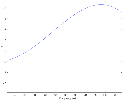
Figure 2: Plot of $g(\omega)$ zoomed

where $K=\frac{NW_{0}^{3}}{2}$. Given the plant, $P$, a PI controller, $C$, is proposed in [2] and an ${\cal H}^{\infty}$ controller is suggested in [6] for the feedback loop in Figure 2. We will consider in this paper a PID controller which has a better performance/robustness than a PI controller and simple structure for implementation compared to ${\cal H}^{\infty}$ controller. A method for tuning of the PID parameters will be given in the next sections. Also, the high frequency dynamics of the system (the delay term in the denominator of $P$) is considered as parasitic dynamics in PI controller design [2]. We will include these effects in the design of PID controllers.

3 Tuning of the PID Parameters

In this section, we will define the controller parameter space such that closed loop system is stable. We will use the method proposed in [10]. This approach separates the parameter space of PID controller into stable and unstable region. The stability of a region is checked by the direct method in [11]. Once the “stable region” determined, the optimal parameters are obtained by a numerical search algorithm: the criterion used here is the minimization of the mixed sensitivity function in the region of admissible parameter values.

3.1 The Feasible PID Parameter Space

For the plant, $P$, of the closed loop system Figure 2 is to be stabilized by the PID controller,

$$C(s)=K_{P}+K_{D}s+\frac{K_{I}}{s}.$$ (3.8)

The triplet $(K_{P},K_{I},K_{D})$ stabilizes the overall system if and only if all the roots of the characteristic equation,

$$CE(s) = sD_{p}(s)+(K_{I}+K_{P}s+K_{D}s^{2})N_{P}(s)$$

$$= (W_{0}R_{0}s^{3}+(W_{0}+1)R_{0}s^{2}+2s)+(KK_{I}+KK_{P}s+(KK_{D}+R_{0})s^{2})e^{-R_{0}s},$$

lie in the open left half plane. The algorithm in [10] offers a parameter space approach to certain class of quasi-polynomials in the form of

$$G(s)=(r_{0}+r_{1}s+r_{2}s^{2})A(s)+B(s)e^{sL},\quad\text{$L>0$}$$ (3.10)

where $A$ and $B$ are polynomials with degrees $m$ and $n$ respectively satisfying $n\geq m+2$. It computes the “stable region” for the triplet $(r_{0},r_{1},r_{2})$. We form the quasi-polynomial as the characteristic equation of our time delayed system in (3.1) as

$$r_{0} = KK_{I},$$ (3.11)

$$r_{1} = KK_{P},$$

$$r_{2} = KK_{D}+R_{0},$$

$$A(s) = 1,$$

$$B(s) = W_{0}R_{0}s^{3}+(W_{0}+1)R_{0}s^{2}+2s,$$

$$L = R_{0}.$$

As explained in [10], a stable quasi-polynomial will be unstable only when a left half plane root transients to right half plane. Since $K_{P}$, $K_{D}$, $K_{I}$ and $h$ change continuously, characteristic equation also changes continuously. Thus, for some $(K_{P},K_{D},K_{I})$ triplet, some roots of (3.1) lie on imaginary axis. From these $(K_{P},K_{D},K_{I})$, we can form the stability boundaries in the parameter space. In [10], these crossings are classified into 3 cases and for our problem the boundaries can be found as:

1. Real Root Boundary (RRB), a root crosses imaginary axis at origin, i.e., $G(0)=0$, the boundary is $r_{0}=0$ line, equivalently, $K_{I}=0$.

2. Infinite Root Boundary (IRB) when a root crosses the imaginary axis at infinity, since $m=0$ and $n=3$, the quasi-polynomial is retarded type $(n>m+2)$ and no infinite root boundary exists.

3. Complex Root Boundary (CRB) when a pair of complex conjugate roots crosses the imaginary axis, i.e., $G(j\omega)=0$, then we can separate real and imaginary parts as,
   

   $$\left[\begin{array}[]{cc}1&-\omega^{2}\\ 0&0\\ \end{array}\right]\left[\begin{array}[]{c}r_{0}\\ r_{2}\\ \end{array}\right]+\left[\begin{array}[]{c}\omega((W_{0}R_{0}^{2}\omega^{2}-2)\sin{R_{0}\omega-(W_{0}+1)R_{0}\omega\cos{R_{0}\omega})}\\ -\omega(W_{0}R_{0}^{2}\omega^{2}-2)\cos{R_{0}\omega-(W_{0}+1)R_{0}\omega\sin{R_{0}\omega}+r_{1})}\\ \end{array}\right]=\left[\begin{array}[]{c}0\\ 0\\ \end{array}\right]$$

   If we fix $r_{1}=r_{1}^{*}$, the solution of the above system of equations exists only for real zeros of $\omega_{gi}$ of

   $$g(\omega)=\omega r_{1}^{*}+(W_{0}R_{0}^{2}\omega^{2}-2)\omega\sin{R_{0}\omega}-(W_{0}+1)R_{0}\omega^{2}\cos{R_{0}\omega}.$$ (3.12)

   Each positive zero corresponds a straight line as CRB in $(r_{2},r_{0})$ plane with equation,

   $$r_{0}=\omega_{gi}^{2}r_{2}-\omega_{g}((W_{0}R_{0}^{2}\omega_{g}^{2}-2)\sin{R_{0}\omega_{g}-(W_{0}+1)R_{0}\omega_{g}\cos{R_{0}\omega_{g}})}.$$ (3.13)

Stability boundaries (RRB, IRB, CRB) can be found as explained above. For each $r_{1}$, we can find a region in $(r_{2},r_{0})$ plane, and for various $r_{1}$ values, we can form a three dimensional region, $\Pi_{r}$. Any triplet in this region as PID parameters (i.e., $(r_{0},r_{1},r_{2})\in\Pi_{r}$) ensures stable closed loop system. Note that actual PID parameters are not the triplet $(r_{0},r_{1},r_{2})$, but $(K_{P},K_{I},K_{D})$. After the region, $\Pi_{r}$, obtained, we can transform to another region, $\Pi_{K}$, for the triplet $(K_{P},K_{I},K_{D})$ by linear transformation in (3.11). Also, in order to check the inside of the region, $\Pi_{K}$, (whether it is stable or not) we used the method in [11], which is not discussed here.

3.2 Computation of the Optimal PID Parameters

We aim to find the optimal PID parameters such that we have robust stability and good tracking for the set point changes. For this purpose we will use the weighted ${\cal H}^{\infty}$ norm of mixed sensitivity function, as our performance metric. Since a PID controller has three parameters, $(K_{P},K_{I},K_{D})$, we can search the optimal triplet, $(K_{P,opt},K_{I,opt},K_{D,opt})$ in $\Pi_{K}$ such that the mixed sensitivity function,

$$\Psi(K_{P},K_{I},K_{D})=\sup_{\omega\in[0,\infty)}\left\{|W_{1}(j\omega)S(j\omega)|^{2}+|W_{2}(j\omega)T(j\omega)|^{2}\right\},$$ (3.14)

attains its minimum value. The weight functions $W_{1}$ and $W_{2}$ are finite dimensional terms as design parameters for robustness and performance. The sensitivity, $S$, and complementary sensitivity, $T$, functions are defined as usual:

$$S(s) = (1+P(s)C(s))^{-1}$$

$$T(s) = P(s)C(s)(1+P(s)C(s))^{-1}$$

where $P$ and $C$ are given in (2.7) and (3.8), respectively. Formally, we can define the numerical search problem as: Find the triplet, $(K_{P,opt},K_{I,opt},K_{D,opt})$ such that

$$\Psi(K_{P,opt},K_{I,opt},K_{D,opt})\leq\Psi(K_{P},K_{I},K_{D}),\quad\forall\;(K_{P},K_{I},K_{D})\in\Pi_{K},$$ (3.15)

the inequality is satisfied. We will simply use a brute force method by taking a grid set in the feasible parameter space.

4 Simulation Results

We have simulated the nonlinear model defined by equations (2.2) and (2.3) for the dynamics of $N$ TCP flows loading a router by using simulink and MATLAB. The numerical values for the simulations are taken to be the same as in [6] for comparison purposes:

• Nominal values known to the controller: $N_{n}=50$ TCP sessions, $C_{n}=300$ packets/sec, $T_{p}=0.2$ sec. Then, by simple calculation $R_{0n}=0.533$ sec and $W_{0n}=3.2$ packets. Desired queue length is $q_{0}=100$ packets.

• Real values of the plant: $N=40$ TCP sessions, $C=250$ packets/sec, $T_{p}=0.3$ sec, which means that we actually have $R_{0}=0.7$ sec and $W_{0}=4.375$ packets.

The above data will be used to check the performance of the overall feedback system. In order to analyze the robustness of closed loop system with respect to variations in the network parameters, the following scenario is considered: outgoing link capacity, $C$, is a normally distributed random signal with mean $250$ packets/sec and variance $50$ added to a pulse of period $60$sec, amplitude $60$ packets/sec. The number of TCP flows $N$ is a normally distributed random signal with mean $45$ and variance $30$ added to a pulse of period $20$ sec and amplitude $10$. The propagation delay $T_{p}$ is a normally distributed random signal with mean $0.8$ sec and variance $0.05$ sec added to a pulse of period $20$ sec and amplitude $0.2$ sec. The controllers have the following values known to them: $C=300$ packets/sec, $N=50$, $T_{p}=0.7$sec and desired queue length is $q_{0}=100$ packets.

4.1 Tuning PID Parameters

For the given network parameters, we can write the characteristic equation from (3.10),

$$G(s) = (r_{0}+r_{1}s+r_{2}s^{2})A(s)+B(s)e^{sL}$$

$$= (r_{0}+r_{1}s+r_{2}s^{2})+(1.706s^{3}+2.239s^{2}+2s)e^{0.533s}$$

$$= (819.2K_{I}+819.2K_{P}s+(819.2K_{D}+0.533)s^{2})+(1.706s^{3}+2.239s^{2}+2s)e^{0.533s}$$

We will work with $(r_{0},r_{1},r_{2})$ triplet and calculate the PID parameters, $(K_{P},K_{D},K_{I})$, at the end. It is clear that for this plant $m=0$ and $n=3$. Also note that $B(s)$ does not contain any constant term. Therefore, we do not encounter any infinite root boundary (IRB) and have always a real root boundary (RRB) which is $r_{0}=0$.

In order to determine complex root boundaries (CRB), we should first decide, over which interval we should sweep fixed $r_{1}$. If we acquire for (3.12), considering the values for $C$, $N$, $W_{0}$, $R_{0}$, we obtain Figure 4. The interval, in which maximum number of $\omega_{gi}$ is produced, can be better observed when we look in the interval, $\omega\in[0,120]$ as in Figure 4. As we easily observed from Figure 4 that it is enough to sweep $r_{1}$ between $[-2,8]$ in our problem. Therefore we obtained the boundary lines for stability on the $(r_{0},r2)$ plane for each fixed $r_{1}$. These boundary lines yield a polygon in which we have stability. After sweeping $r_{1}$ and combining all polygons, we obtain the stability space for controller parameters.

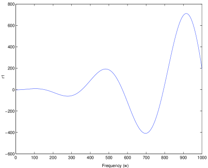
Figure 1: Plot of $g(\omega)$

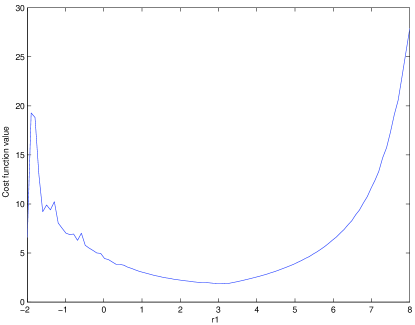
Figure 3: Plot of $\Psi$

Figure 4: Plot of the region when $r_{1}^{*}=3.15$

The region shown in Figure 4 is robust to small variations (about 10%) in the original problem data, $N$, $T_{p}$, $C_{n}$, as shown above.

In order to find the optimal PID parameters, we define the cost function, $\Psi$, with weight functions,

$$W_{1}(s) = \frac{1+0.01s}{0.01+s},$$

$$W_{2}(s) = s+1.$$

In Figure 4, for fixed $r_{1}\in[-2,8]$, the minimum value of cost function in $(r_{0},r_{2})$ plane is given. The minimum value is achieved at $r_{1,opt}=3.15$. Figure 4 shows the controller parameter space in $(r_{0},r_{2})$ plane when $r_{1}=3.15$. The optimal point is found as $r_{1,opt}=3.15$, $r_{2,opt}=2.2460$ and $r_{0,opt}=1.2189$. These normalized values correspond to the $K_{P.opt}=3.845\;10^{-3}$, $K_{D,opt}=2.091\;10^{-3}$ and $K_{I,opt}=1.48\;10^{-3}$. The location of optimal, center and one of the boundary points can be seen in Figure 4.

4.2 Performance and Robustness of the Feedback System

Once the optimal point is found, we need to simulate the feedback system to check the performance of our controller. In [6], the performance of ${\cal H}^{\infty}$ and PI controllers are compared. Using the simulation parameters of [6] (given above), we obtained Figure 6, from which the comparison between our PID, ${\cal H}^{\infty}$ and $PI_{1}$ and $PI_{2}$ controllers can be made.

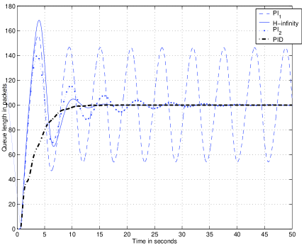
Figure 5: Performance comparison of PID, ${\cal H}^{\infty}$, $PI_{1}$ and $PI_{2}$ controllers

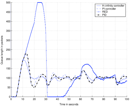
Figure 6: Robustness comparison of PID, ${\cal H}^{\infty}$, $PI_{1}$ and $PI_{2}$ controllers

Figure 6 reveals that PID controller responds better than other controllers. Although rise time is longer, settling time of PID is shorter than the other ones. Also note that there is no overshoot for the proposed PID controller.

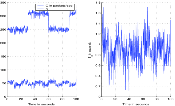
Figure 7: Values of $C$, $N$ and $T_{p}$ corresponding to Figure 6

For variation in network parameters as shown in Figure 7, robust performance of our global optimum point is obtained in Figure 6. We observe that the PID controller which we design using the method introduced in [10] has similar robust performances with other proposed controllers of [2, 6].

4.3 Remarks

1) Since PID controller design is based on linearization of nonlinear plant, we may encounter different points in the stable space which give us better performance and robustness. For example, in our simulations, the results of a PID controller with parameters $r_{1}=1$, $r_{2}=0.7016$ and $r_{0}=0.839$ ($K_{P}=1.221\;10^{-3}$, $K_{D}=2.054\;10^{-4}$ and $K_{I}=1.024\;10^{-3}$) are given in Figure 9 and 9. It can be seen that the controller has a better settling and rise time with an overshoot. However, the robust performance of optimal point is better than the point ($r_{1}=1$, $r_{2}=0.7016$ and $r_{0}=0.839$).

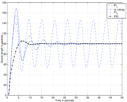
Figure 8: Performance comparison of when $r_{1}=1$, $r_{2}=0.7016$ and $r_{0}=0.839$

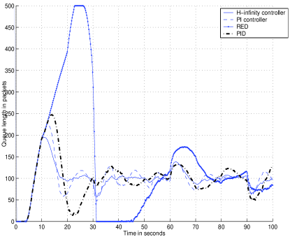
Figure 9: Robustness comparison of when $r_{1}~{}=~{}1$, $r_{2}=0.7016$ and $r_{0}=0.839$

2) For confirmation we performed several other simulations for the following points in the parameter space: (i) center of the stability polygon, (ii) the boundary of the stability polygon (shown with diamond and circle symbol in Figure 4), which we think intuitively that, they yield stable and unstable responses, respectively.

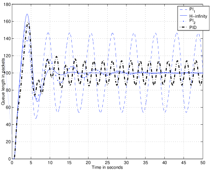
Figure 10: Performance comparison of central point

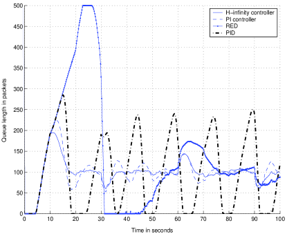
Figure 11: Robustness comparison of central point

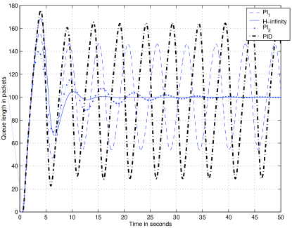
Figure 12: Performance comparison of boundary point

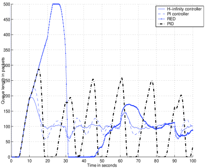
Figure 13: Robustness comparison of boundary point

Figure 13 and 13 show the responses of the center and the boundary point respectively for the r1=3.15 polygon. We can see that stability is violated as we move to the boundary, which is naturally expected. This violation can also be observed from the robust performance of the boundary in 13. The robust performance difference is very significant when we compare Figure 6 and 13. For the boundary, the robust response in queue length deviates in $[0,250]$, unlikely for the optimal point, this deviation is in $[50,140]$.

5 Concluding Remarks

We proposed a PID controller for robust AQM control scheme supporting TCP flows. Tuning algorithm for this PID controller is based on [10, 11] and a numerical search algorithm for minimization of mixed sensitivity cost function. We compared our controller performance and robustness with other controllers studied in [2, 6]. For the application on AQM supporting TCP flows, we obtained relatively good performances compared to RED, $PI_{1}$ and $PI_{2}$ controllers by achieving fast transients and low oscillatory behavior.

References

- [1] V. Misra, W. B. Gong, and D. Towsley, “Fluid-based analysis of a network of AQM routers supporting TCP flows with an application to RED,” Proc. of ACM/SIGCOMM, pp. 151–160, 2000.
- [2] C. V.Hollot, V. Misra, D. Towsley, and W. B. Gong, “Analysis and design of controllers for AQM routers supporting TCP flows,” IEEE Trans. on Auto. Cont., vol.47, pp.945–959, June 2002.
- [3] F. Kelly, Mathematical modelling of the Internet” in Mathematics Unlimited - 2001 and Beyond (B. Engquist and W. Schmid, eds.), Springer-Verlag, Berlin, 2001.
- [4] S. Mascolo, “Modeling the internet congestion control as a time delay system: a robust stability analysis,” Proc. of 4th IFAC Workshop on Time Delay Systems, Rocquencourt, France, September 2003.
- [5] H-F Reynaud, C. Kulcsar, R. Hammi, “In communication networks there are delays, delays, …and delays,” Proc. of 4th IFAC Workshop on Time Delay Systems, Rocquencourt, France, September 2003.
- [6] P-F. Quet, and H. Ozbay, “On the Design of AQM Supporting TCP Flows Using Robust Control Theory,” Proc. of the 42nd IEEE Conf. on Decision and Cont., Maui, Hawaii, December 2003.
- [7] Y. Fan, F. Ren, C. Lin, “Design a PID Controller for Active Queue Management,” Proc. of the 8th IEEE Symp. on Computers and Communications, Kemer, Antalya, Turkey, June-July 2003, pp.985–990.
- [8] S. Ryu, C. Rump, C. Qiao, “A Predictive and robust Active Queue Management for Internet Congestion Control,” Proc. of the 8th IEEE Symp. on Computers and Communications, Kemer, Antalya, Turkey, June-July 2003, pp.991-998.
- [9] E. Plasser, T. Ziegler, “An Analytical RED function design guaranteeing stable system behavior,” Proc. of the 8th IEEE Symp. on Computers and Communications, Kemer, Antalya, Turkey, June-July 2003, pp.1012-1017.
- [10] N. Hohenbichler, J. Ackermann, “Computing stable regions in parameter spaces for a class of quasipolynomials,” Proc. of 4th IFAC Workshop on Time Delay Systems, Rocquencourt, France, September 2003.
- [11] N. Olgac, R. Sipahi, “Direct method for analyzing the stability of neutral type LTI time delayed systems,” Proc. of 4th IFAC Workshop on Time Delay Systems, Rocquencourt, France, September 2003.