A Non-stationary Thermal-Block Benchmark Model for Parametric Model Order Reduction

Abstract

In this contribution we aim to satisfy the demand for a publicly available benchmark for parametric model order reduction that is scalable both in degrees of freedom as well as parameter dimension.

1 Introduction

Model order reduction (MOR) of parametric problems (PMOR) is accepted to be an important field of research, in particular due to its relevance for multi-query applications such as uncertainty quantification, inverse problems or parameter studies in the engineering sciences. Still, publicly available software is often either tailored to a very specific problem or bound to a specific PDE discretization software. The joint feature of the software packages, emgr [13], M-M.E.S.S. [23], MORLAB [7] and pyMOR [18], reported in this volume is the attempt to make (P)MOR available in a more general purpose fashion. Further packages that fall into this category are rbMIT [17], RBmatlab [21, 11], RBniCS [5, 12], redbKIT [16, 19], psssMOR [8]. So far, comparison of PMOR methods is a difficult task [6]. We think that one of the difficulties is the lack of models that can be easily used and fairly compared in all packages. It is the goal of this benchmark to overcome some of the shortcomings of available benchmarks.

The MOR community Wiki [24] already provides a number of parametric benchmark models. However, most of them have either rather large dimensions making them difficult to access directly for dense matrix-based packages like [7], but also cumbersome to use during development and testing of new sparse methods. Other benchmarks have rather limited parameter dimension, i.e. they feature only scalar or at most two-dimensional parameters. A very common feature among the benchmarks in the Wiki is that essentially all of them are matrix-based, giving easy access for MATLAB^®-based solvers, but at the same time making it difficult for packages like pyMOR [18, 15, 3] to show their full flexibility.

Therefore, the new benchmark introduced in this chapter has a few features addressing exactly these problems. The model is of limited dimension in the basic version provided as matrices. On the other hand, it also provides the FEniCS [1, 14] based procedural setup allowing for easy generation of larger versions or integration into FEniCS-based software packages. The current version features one to four parameters, but the setup can be extended to higher parameter dimensions by tweaking the basic domain description given as plain text input for gmsh [10]. Thus, we provide maximal flexibility with a small, but scalable benchmark with up to four independent parameters given in a description that can easily be adapted for many PDE discretization tools. The benchmark we introduce here is a specific version of the so called thermal-block benchmark. This type of model has been a standard test case in the reduced basis community for many years, e.g. [22]. This specific model setup is also known as the “cookie baking problem” [4] in the numerical linear algebra community. It further presents a flattened 2d version of what is sometimes referred to as the “skyscraper model” in high performance computing, e.g. [9, p. 216]. We choose the common name used for this type of model in the reduced-basis community.

The remainder of this chapter is organized as follows. The next section provides a basic, abstract description of the model problem. After that, in Section 3, we present three variants of our model that will be used in the numerical experiments of the following chapters.

2 Problem Description

Figure 1: computational domain and boundaries

We consider a basic parabolic ‘thermal-block’-type benchmark problem. To this end, consider the computational domain $\Omega:={(0,1)}^{2}$ which we partition into subdomains

$$\Omega_{1} :=\{\xi\in\Omega\ |\ |\xi-(0.3,0.3)|<0.1\}, \Omega_{2} :=\{\xi\in\Omega\ |\ |\xi-(0.7,0.3)|<0.1\},$$

$$\Omega_{3} :=\{\xi\in\Omega\ |\ |\xi-(0.7,0.7)|<0.1\}, \Omega_{4} :=\{\xi\in\Omega\ |\ |\xi-(0.3,0.7)|<0.1\},$$

$$\Omega_{0} :=\Omega\setminus(\Omega_{1}\cup\Omega_{2}\cup\Omega_{3}\cup\Omega_{4}),$$

with its boundary partitioned into

$$\Gamma_{in}:=\{0\}\times(0,1),\quad\Gamma_{D}:=\{1\}\times(0,1),\quad\Gamma_{N}:=(0,1)\times\{0,1\},$$

cf. Fig. 1. Given a parameter $\mu\in\mathbb{R}_{\geq 0}^{4}$, let the heat conductivity $\sigma(\xi;\mu)$ given by

$$\sigma(\xi;\mu):=\begin{cases}1&\xi\in\Omega_{0}\\ \mu_{i}&\xi\in\Omega_{i},\quad 1\leq i\leq 4,\end{cases}$$ (1)

and let the temperature $\theta(t,\xi;\mu)$ in the time interval $[0,T]$ for thermal input $u(t)$ at $\Gamma_{in}$ be given by

$$\partial_{t}\theta(t,\xi;\mu)+\nabla\cdot(-\sigma(\xi;\mu)\nabla\theta(t,\xi;\mu)) =0 t\in(0,T), \ \xi\in\Omega,$$

$$\sigma(\xi;\mu)\nabla\theta(t,\xi;\mu)\cdot n(\xi) =u(t) t\in(0,T), \ \xi\in\Gamma_{in},$$

$$\sigma(\xi;\mu)\nabla\theta(t,\xi;\mu)\cdot n(\xi) =0 t\in(0,T), \ \xi\in\Gamma_{N},$$

$$\theta(t,\xi;\mu) =0 t\in(0,T), \ \xi\in\Gamma_{D},$$

$$\theta(0,\xi;\mu) =0 \ \xi\in\Omega.$$

More precisely, we let $\theta\in L^{2}(0,T;V)$ with $\partial_{t}\theta(\mu)\in L^{2}(0,T;V^{\prime})$ be given as the solution of the weak parabolic problem

$$\langle\partial_{t}\theta(t,\cdot;\mu),\,v\rangle+\int_{\Omega}\sigma(\mu)\nabla\theta(t,\xi;\mu)\cdot\nabla v\operatorname{d\!}\xi =\int_{\Gamma_{in}}u(t)v\operatorname{d\!}s t\in(0,T), \ v\in V,$$ (2)

$$\theta(0,\xi;\mu) =0,$$ (3)

where $V:=\{v\in H^{1}_{0}(\Omega)\ |\ v_{\Gamma_{D}}=0\}$ denotes the space of Sobolev functions with vanishing trace on $\Gamma_{D}$ and $V^{\prime}$ is its continuous dual.

As outputs $y(t;\mu)\in\mathbb{R}^{4}$ we consider the average temperatures in the subdomains $\Omega_{i}$, i.e.

$$y_{i}(t;\mu):=\frac{1}{|\Omega_{i}|}\int_{\Omega_{i}}\theta(t,\xi;\mu)\operatorname{d\!}\xi,\qquad 1\leq i\leq 4.$$ (4)

To ease the notation, we drop the explicit dependence on $\xi$ in the following.

In view of the definition (1) of $\sigma$ as a linear combination of characteristic functions, we can write (2)–(4) as

$$\partial_{t}m(\theta(t;\mu),v)+a_{0}(\theta(t;\mu),v)+\sum_{i=1}^{4}\mu_{i}\cdot a_{i}(\theta(t;\mu),v) =\varphi(v)\cdot u(t)\in V$$ (5)

$$\theta(0;\mu) =0$$

$$y_{i}(t;\mu) =\psi_{i}(\theta(t;\mu)),$$

for $t\in(0,T)$, $v\in V$, $1\leq i\leq 4$, with bilinear forms $m,a_{i}\in\operatorname{Bil}(V,V)$ given by

$$m(w,v):=\int_{\Omega}wv\operatorname{d\!}\xi\quad\text{and}\quad a_{i}(w,v):=\int_{\Omega_{i}}\nabla w\cdot\nabla v\operatorname{d\!}\xi$$

and linear forms $\varphi,\psi_{i}\in V^{\prime}$ given by

$$\varphi(v):=\int_{\Gamma_{in}}v\operatorname{d\!}s,\quad\text{and}\quad\psi_{i}(v):=\frac{1}{|\Omega_{i}|}\int_{\Omega_{i}}v\operatorname{d\!}\xi.$$

To arrive at a discrete approximation of (5), we perform a Galerkin projection onto a space $S^{1}(\mathcal{T})\cap V$ of linear finite elements w.r.t. a simplicial triangulation of $\Omega$ approximating the decomposition into the subdomains $\Omega_{0},\ldots,\Omega_{4}$. Assembling matrices $E\in\mathbb{R}^{n\times n}$ for $m$, $A_{i}\in\mathbb{R}^{n\times n}$ for $a_{i}$, $B\in\mathbb{R}^{n\times 1}$ for $\varphi$, and $C\in\mathbb{R}^{4\times n}$ for $\psi_{i}$, all w.r.t. the finite-element basis we arrive at the linear time-invariant system

$$E\cdot\partial_{t}x(t;\mu) =A_{0}\cdot x(t;\mu)+\sum_{i=1}^{4}\mu_{i}A_{i}\cdot x(t;\mu)+B\cdot u(t)$$ (6)

$$y(t;\mu) =C\cdot x(t;\mu).$$

Here, $n$ denotes the dimension of the finite-element space and $x$ is the coefficient vector of the discrete solution state $\theta$ w.r.t. the finite-element basis.

For the numerical experiments in the following chapters, the mesh $\mathcal{T}$ was generated with gmsh version 3.0.6 with ‘clscale’ set to $0.1$, for which the system matrices were assembled using FEniCS 2019.1.

The source code of the model implementation as well as the resulting system matrices are available at https://doi.org/10.5281/zenodo.3691894

Note that due to the handling of Dirichlet constraints in FEniCS, all matrices were assembled over the full unconstrained space $S^{1}(\mathcal{T})$. Rows of $E,A_{i}$ corresponding to degrees of freedom located on $\Gamma_{D}$ have zero off-diagonal entries. The corresponding diagnal entries are $1$ for $E$, $-1$ for $A_{0}$ and $0$ for $A_{1},\ldots,A_{4}$. Rows of $B$ corresponding to Dirichlet degrees of freedom are set to 0. Consequently, all system matrices $A(\mu):=A_{0}+\sum_{i=1}^{4}\mu_{i}A_{i}$ have a $k$ dimensional eigenspace with eigenvalue $-1$ spanned by the $k$ finite-element basis functions associated with $\Gamma_{D}$.

3 Problem Variants

The following chapters test the model introduced in the previous section in three different variants. The simplest case is a basic non-parametric version with all parameters fixed. For the parametric versions either all four parameters are considered independent, or they are all scaled versions of a single scalar parameter. This section introduces all of them with the specific parameter selections and allowed parameter domains.

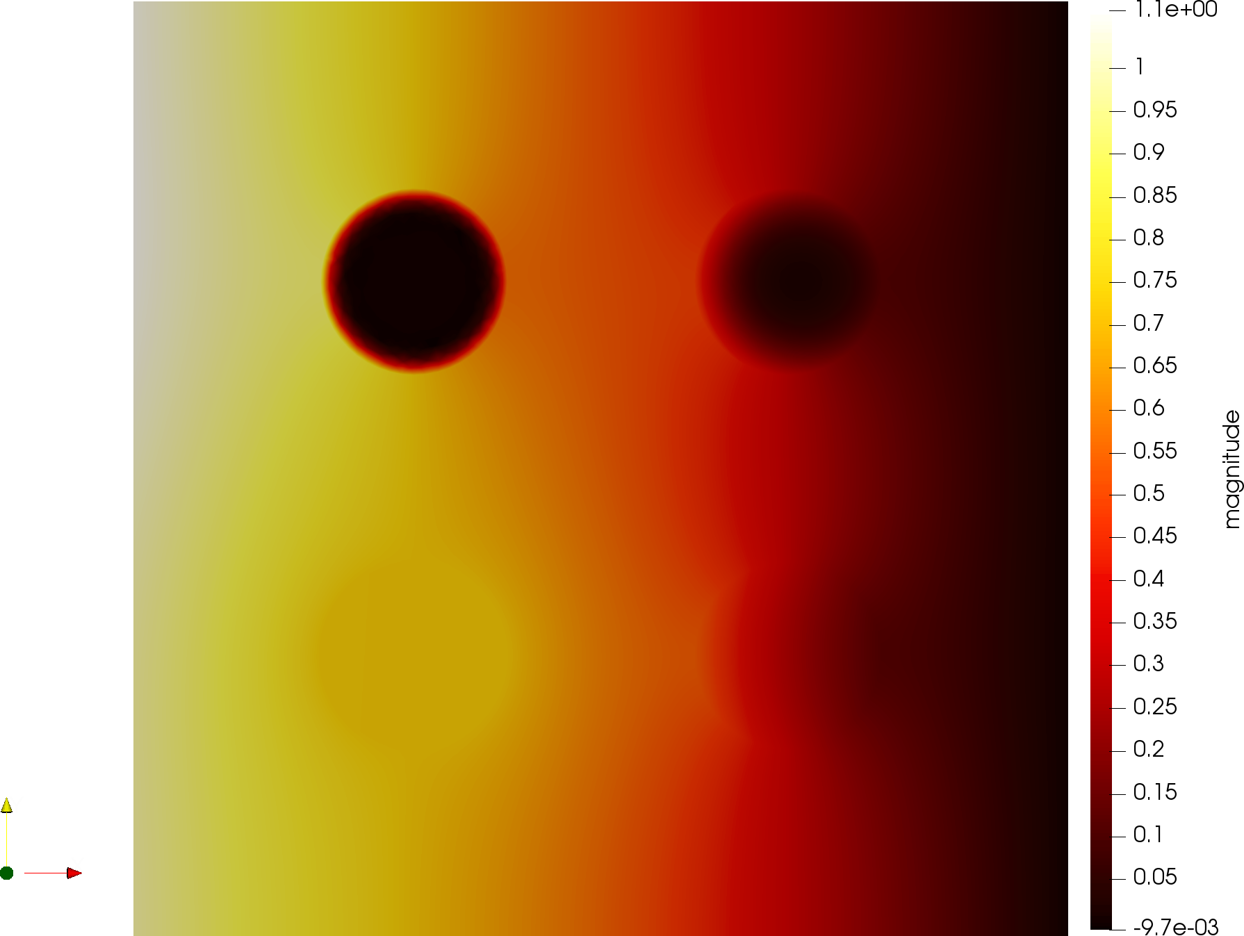
Figure 2: A sample final heat distribution.

3.1 Four Parameter LTI System

This represents exactly the model in (5), or (6), with its full flexibility with respect to the parameters. Note that by construction the model becomes singular in case any of the $\mu_{i}$ become zero. Thus, we limit the $\mu_{i}$ from below by $10^{-6}$. This will also limit the condition numbers of the linear systems involving the matrices $E$ and $A_{i}$ ($i=0,\dots,4$) in the PDE solvers as well as MOR routines. At the same time, we do not allow for the subdomain heat conductivities to be drastically larger than the conductivity for $\Omega_{0}$. So we limit also from the above, resulting in parameter domains $\mu_{i}\in[10^{-6},10^{2}]$, ($i=1,\dots,4$).

Figure 2 shows the final heat distribution, at $t=1$ after 100 steps of implicit Euler with $\mu=[10^{2},10^{-2},10^{-3},10^{-4}]$, in pyMOR 2019.2.

3.2 Single Parameter LTI System

graphics/FOM_sigma.tikzfigures/FOM_sigma.pdf

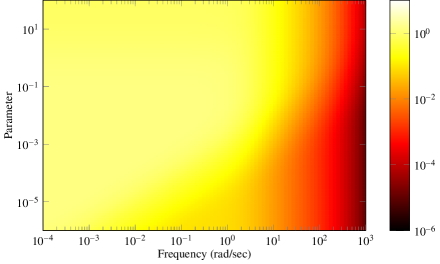
Figure 3: Sigma magnitude plot for the single parameter LTI system.

In this variation of the model the parameters are limited in flexibility. We make them all use the same order of magnitude by defining

$$\mu=\tilde{\mu}\cdot\begin{bmatrix}0.2\\ 0.4\\ 0.6\\ 0.8\end{bmatrix},$$

for a single scalar parameter $\tilde{\mu}\in[10^{-6},10^{2}]$. The transfer function, arising after Laplace transformation of (6) is a rational matrix-valued function of the frequency and the parameters. Its Sigma-magnitude plot, i.e. the maximum singular value of the transfer function matrix, with this restriction on $\mu$, is shown in Figure 3.

3.3 Non-parametric LTI System

This is the simplest version of the benchmark. We use the setup described in Section 3.2 with $\tilde{\mu}=\sqrt{10}$. Note that this value of $\tilde{\mu}$ is rather arbitrary. Depending on the desired application, different values may be insightful. For both time domain and frequency domain investigations variation is strongest in the parameter range $[10^{-5},10^{-1}]$. On the other hand values between $1.25$ and $5.0$ essentially turn the model into a simple heat equation on the unit square with almost homogeneous heat conductivity $\sigma(t,\xi,\tilde{\mu})\approx 1$. Hence, $\tilde{\mu}=\sqrt{10}\approx 3.1623$ appears to be a proper choice to get reasonably close to an easy to solve textbook problem, here. Smaller values of $\mu$, especially when approaching $\mu=0$, can be used to make the problem arbitrarily ill conditioned.

Conclusion

We have specified a flexible, scalable benchmark that can be used both based on pre-generated matrices or based on a procedural inclusion into an existing finite element setting. The new model has been added to the benchmark collection hosted at the MOR Wiki [24, Thermal Block].

References

- [1] M. S. Alnæs, J. Blechta, J. Hake, A. Johansson, B. Kehlet, A. Logg, C. Richardson, J. Ring, M. E. Rognes, and G. N. Wells. The FEniCS project version 1.5. Archive of Numerical Software, 3(100):9–23, 2015.
- [2] Martin S. Alnæs. UFL: a Finite Element Form Language, chapter 17. Springer, 2012.
- [3] L. Balicki, P. Mlinarić, S. Rave, and J. Saak. System-theoretic model order reduction with pyMOR. Proc. Appl. Math. Mech., 19(1), 2019.
- [4] J. Ballani and D. Kressner. Reduced basis methods: From low-rank matrices to low-rank tensors. SIAM J. Sci. Comput., 38(4):A2045–A2067, 2016.
- [5] F. Ballarin and G. Rozza. RBniCS. https://mathlab.sissa.it/rbnics.
- [6] U. Baur, P. Benner, B. Haasdonk, C. Himpe, I. Martini, and M. Ohlberger. Comparison of methods for parametric model order reduction of time-dependent problems. In P. Benner, A. Cohen, M. Ohlberger, and K. Willcox, editors, Model Reduction and Approximation: Theory and Algorithms, pages 377–407. SIAM, 2017.
- [7] P. Benner and S. W. R. Werner. MORLAB – Model Order Reduction LABoratory (version 5.0), 2019. see also: http://www.mpi-magdeburg.mpg.de/projects/morlab.
- [8] Chair of Automatic Control TUM, Technical University of Munich. psssMOR. https://www.mw.tum.de/rt/forschung/modellordnungsreduktion/software/psssmor/.
- [9] V. Dolean, P. Jolivet, and F. Nataf. An introduction to domain decomposition methods. Society for Industrial and Applied Mathematics (SIAM), Philadelphia, PA, 2015. Algorithms, theory, and parallel implementation.
- [10] C. Geuzaine and J.-F. Remacle. Gmsh Reference Manual, October 2010. http://www.geuz.org/gmsh/doc/texinfo/gmsh.pdf.
- [11] B. Haasdonk. Reduced Basis Methods for Parametrized PDEs—A Tutorial Introduction for Stationary and Instationary Problems, chapter 2, pages 65–136. SIAM Publications, 2017.
- [12] Jan S Hesthaven, Gianluigi Rozza, and Benjamin Stamm. Certified Reduced Basis Methods for Parametrized Partial Differential Equations. SpringerBriefs in Mathematics. Springer International Publishing, 1 edition, 2016.
- [13] C. Himpe. emgr – EMpirical GRamian framework (version 5.4). http://gramian.de, 2018.
- [14] A. Logg, K.-A. Mardal, and G. Wells, editors. Automated Solution of Differential Equations by the Finite Element Method, volume 84 of Lect. Notes Comput. Sci. Eng. Springer-Verlag, 1 edition, 2012.
- [15] R. Milk, S. Rave, and F. Schindler. pyMOR – generic algorithms and interfaces for model order reduction. SIAM J. Sci. Comput., 38(5):S194–S216, 2016.
- [16] F. Negri. redbKIT Version 2.2. http://redbkit.github.io/redbKIT/, 2016.
- [17] A.T. Patera and G. Rozza. Reduced basis approximation and a posteriori error estimation for parametrized partial differential equations. Version 1.0, Copyright MIT 2006, https://orms.mfo.de/project?id=316.
- [18] pyMOR developers and contributors. pyMOR - model order reduction with Python. https://pymor.org.
- [19] Alfio Quarteroni, Andrea Manzoni, and Federico Negri. Reduced Basis Methods for Partial Differential Equations, volume 92 of La Matematica per il 3+2. Springer International Publishing, 2016.
- [20] F. Rathgeber, D. A. Ham, L. Mitchell, M. Lange, F. Luporini, A. T. T. McRae, G.-T. Bercea, G. R. Markall, and P. H. J. Kelly. Firedrake: automating the finite element method by composing abstractions. ACM Trans. Math. Softw., 43(3):24:1–24:27, 2016.
- [21] RBmatlab. https://www.morepas.org/software/rbmatlab/.
- [22] G. Rozza, D. B. P. Huynh, and A. T. Patera. Reduced basis approximation and a posteriori error estimation for affinely parametrized elliptic coercive partial differential equations. Archives of Computational Methods in Engineering, 15(3):229–275, 2008.
- [23] J. Saak, M. Köhler, and P. Benner. M-M.E.S.S. – the matrix equations sparse solvers library. see also: https://www.mpi-magdeburg.mpg.de/projects/mess.
- [24] The MORwiki Community. MORwiki - Model Order Reduction Wiki. http://modelreduction.org.