Addressing Target Shift in Zero-shot Learning
using Grouped Adversarial Learning

Abstract

Zero-shot learning (ZSL) algorithms typically work by exploiting attribute correlations to be able to make predictions in unseen classes. However, these correlations do not remain intact at test time in most practical settings and the resulting change in these correlations lead to adverse effects on zero-shot learning performance. In this paper, we present a new paradigm for ZSL that: (i) utilizes the class-attribute mapping of unseen classes to estimate the change in target distribution (target shift), and (ii) propose a novel technique called grouped Adversarial Learning (gAL) to reduce negative effects of this shift. Our approach is widely applicable for several existing ZSL algorithms, including those with implicit attribute predictions. We apply the proposed technique (gAL) on three popular ZSL algorithms: ALE, SJE, and DEVISE, and show performance improvements on 4 popular ZSL datasets: AwA2, aPY, CUB and SUN. We obtain SOTA results on SUN and aPY datasets and achieve comparable results on AwA2.

1 Introduction

Zero-shot learning (ZSL) algorithms are designed to train classifiers using examples of seen classes to be able to generalize and predict any set of unseen classes [29, 35]. Such models generalize by utilizing additional information, specifically, semantically relevant mid-level attributes that (are assumed to) persist between seen and unseen classes. Hence, the performance of a ZSL model is governed by its ability to predict these persistent attributes in instances of unseen classes. The standard view of ZSL assumes class-attribute mapping for the test classes is available only at inference time. On the other hand, the transductive ZSL represents a relaxed view [14, 43] that allows for unlabelled test set as unsupervised additional information. However, obtaining a significant number of instances from unseen classes of interest is not always feasible.

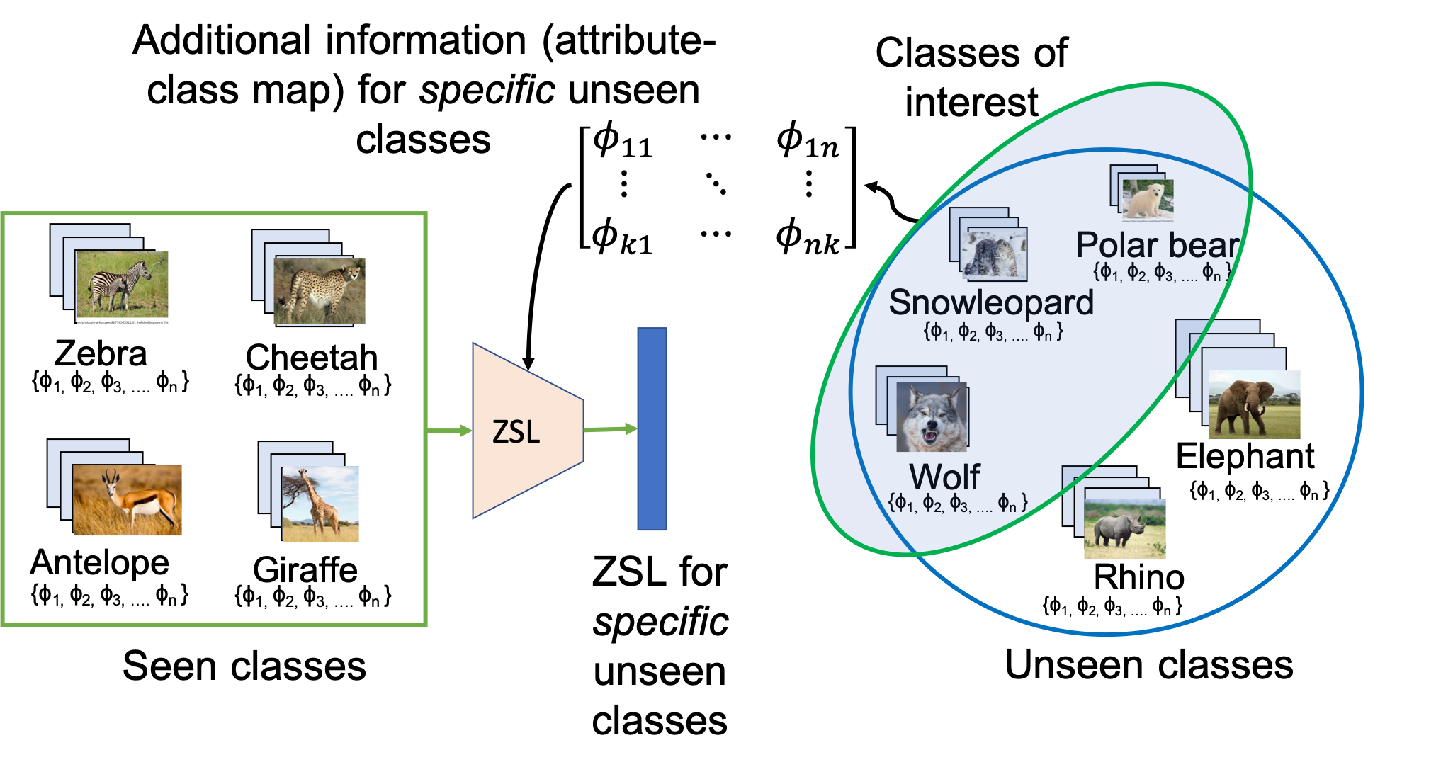
Figure 1: Our approach to Zero shot learning uses attribute class map for the specific unseen classes to minimize target shift.

In ZSL, attribute correlations are useful when the expected label correlation of unseen classes remain consistent with that of train classes. However, we observed that a key reason for the practical difficulty of predicting attributes from instances of unseen classes is the adverse effect of those attribute correlations that are highly likely to change in the test set, we term this effect correlation shift. When the attribute predictors of ZSL are viewed as an instance of multilabel classification, the change in the attribute distribution may be viewed with the lens of domain adaptation literature as target shift [31]. However, existing target shift correction techniques from domain adaptation use importance reweighting, which is not applicable to ZSL (see detail in Sec.3.1), the shift in correlation between the attributes can be considered as one aspect of target shift. We hypothesize that it is necessary to estimate correlation among attributes in test set to correct correlation shift. We propose to use class-attribute vectors of test classes to estimate test correlation.

In the low-resource scenario of ZSL, it is pragmatic to leverage the more readily available additional information about the attribute space. It is much easier to construct a class-attribute mapping of test classes by utilizing class descriptions from auxiliary sources such as knowledge bases (e.g. Wikipedia). For example, to train a ZSL image classifier for the rare and endangered Red Wolf animal, it would be easier to find attributes describing it such as {slender-legged, large, carnivorous, long-ears} from common sources rather than obtaining several samples of Red Wolf images.

To the best of our knowledge, this is the first work which addresses the phenomenon of correlation shift (as an aspect of target shift) in zero shot learning. The contributions of this work are as follows: (i) As illustrated in Fig.1, we present a new zero-shot learning paradigm where the classifier can be tailored to a specific set of unseen classes by only utilizing additional information such as attribute-class mapping. Specifically, we show that the proposed framework is effective in curtailing correlation shift (as an aspect of target shift) between attributes of seen and unseen classes. (ii) Building on a principled analysis on a controlled synthetic dataset, we propose grouped adversarial learning (gAL) paradigm for correlation shift that is universally applicable to any attribute-prediction based ZSL architecture that is end-to-end trainable. We demonstrate performance improvements with gAL with three popular ZSL algorithms: ALE [1], DEVISE [11] and SJE [2] on four standard zero-shot learning benchmarks, namely, Animals-with-Attributes-2 (AwA2) [49], Attribute Pascal and Yahoo (aPY) [10], Scene UNderstanding (SUN) [51], and Caltech UCSD Birds (CUB) [47] datasets. (iii) Finally, we release a new experimental benchmark (train-test split) that maximizes correlation-shift between the seen and unseen classes to amplify the problem of correlation shift.

2 Related Work

Zero Shot Learning: Zero shot learning has been extensively studied in recent years [49, 36, 27, 42, 4, 34, 45, 3]. Existing methods in ZSL can be broken down into the following categories : i) intermediate attribute classifiers [29], ii) bilinear compatibility frameworks that treat zero-shot recognition as a ranking problem [1, 2, 11], iii) linear closed-form solutions optimized by a ridge regression or mean-squared error objective [36, 27], iv) non-linear compatibility frameworks [3, 48, 41], v) hybrid models [46, 34, 4, 58], and vi) generative models [50, 38, 21, 28, 6] based on GANs[17] or VAE[26] that synthesize images for unseen classes during training. Xian et al.[49] performed an extensive benchmarking of several such algorithms under a common benchmark protocol, representation vectors and hyper-parameter tuning, and showed that the performance of linear compatibility models are comparable with the more complex joint representation-based hybrid models. In a slightly different line of work, some approaches [57, 30, 40] propose techniques to tackle the now well-known hubness problem in ZSL, created by projecting seen and unseen class image features to the attribute (semantic) space. Besides inductive and conventional ZSL, there exists an extensive line of work on transductive [43, 12, 13] and generalized ZSL [5, 28, 33, 39, 21] as well. However, such approaches are not the focus of this work.

Target shift: Previous literature on target shift [56, 31, 32] utilize importance re-weighting over training instances to match the probability of train set with that of test set. This process performs poorly when the cardinality of label set is large (curse of dimensionality). This setting also assumes that instances of labels in test set should strictly be a subset of that of train set (see Sec.3.2). This is not the case in zero shot learning, where different label (attribute) combinations define a class, and train and test sets have different groups of classes.

Label correlation: Addressing the negative effects of label correlations has been previously explored in the areas of machine learning under various terms: debiasing [55, 52, 54], privacy preservation literature [18, 22, 8], and multi-task learning [59, 37, 24]. De-biasing and privacy preservation settings are interested in protected variables or sensitive/private variables that are correlated with the desired label. In multitask learning (MTL), several regularization based methods are proposed to mitigate negative effects of label correlation [59, 24, 37] which attempt to decorrelate label predictors using special regularizers that enforce predictors of different labels to use non-overlapping set of features. The overall intent of these techniques is to decorrelate a multi label classification model. However, such regularizers are not applicable for learned features with end-to-end trainable neural networks.

3 Proposed Framework

3.1 Problem Formulation

Notations and problem setup for ZSL: Given a seen dataset $\mathcal{D}^{s}=\{(x_{i}^{s},y_{i}^{s})\}_{i=1}^{N}$ of $N$ points where $x_{i}^{s}\in\mathcal{X}$ denotes the instance and $y_{i}^{s}$ denotes class label from seen classes $y_{i}^{s}\in\mathcal{Y}^{s}$. For the ZSL problem setup, the aim is to build a model, which trained on $\mathcal{D}^{s}$, can classify instances of unseen classes $x_{i}^{u}$ with labels $y_{i}^{u}\in\mathcal{Y}^{u}$, where $\mathcal{Y}^{s}$ and $\mathcal{Y}^{u}$ are disjoint. Apart from instances and class labels, for every class $y\in\mathcal{Y}^{s}\cup\mathcal{Y}^{u}$, we are provided with $D$ dimensional class-attribute vector $\phi^{y}\in\{0,1\}^{D}$, where $\phi^{y}_{m}=1$ if $m$-th attribute is present in class $y$, otherwise $0$. Attribute vectors connect seen and unseen classes in the semantic space that aids in inference during test time. We use $\Phi^{s}=\{\phi^{y}\}_{y\in\mathcal{Y}^{s}}$ to denote set of class-attribute vectors of seen classes and $\Phi^{u}$ to denote that of unseen classes. Note that we use train with seen and test with unseen interchangeably in this paper.

Attribute target shift : In this work, we focus on those ZSL algorithms that map input instances to attributes either explicitly or implicitly. Given an input instance ($x$), an explicit model predicts binary attribute vector ($\widehat{\phi}(x)$) whereas implicit methods provide soft scores for each attribute ($\widehat{\phi}(x)\in\mathbb{R}^{D}$). $c$ is predicted as the class for an instance if attribute vector $\phi^{c}$ is most compatible with predicted attribute vector $\widehat{\phi}(x)$. Emphasizing only on the task of predicting attributes of instances, we view ZSL as a special case of transfer learning for multilabel classification where the attribute distributions ($P_{\phi}$) differ from seen to unseen classes. We view the change in the attribute distributions ($P_{\phi}$) as domain adaptation under target shift [32, 53, 31], where attribute marginals for the training set (seen classes $P^{s}_{\phi}$) and that for test set (unseen classes $P^{u}_{\phi}$) are different while, conditionals $P_{X|\phi}$ remain the same. Since correcting for target shift requires $P^{u}_{\phi}$ along with the training data, we use set of attribute vectors of unseen classes $\Phi^{u}$ to estimate $P^{u}_{\phi}$ by assuming that all unseen classes are equally likely in the test set. We could also estimate $P^{u}_{\phi}$ from unlabelled test data using Black Box Shift Estimation (BBSE) [32], however, obtaining unlabelled test instances changes the problem setting to transductive-ZSL, which is beyond the current scope.

Existing approaches to correct target shift, such as importance re-weighting [9, 56], match attribute distributions of train and test set by appropriately weighing each instance by $P^{u}_{\phi}/P^{s}_{\phi}$ in the loss function. However, importance re-weighting can’t be extended to ZSL since attribute vector $\phi$ in train set do not appear in the test set essentially letting all the weights be zero ($P^{u}_{\phi}=0$ for all $P^{s}_{\phi}>0$).

3.2 Adversarial learning to address Target Shift

We begin the description of our approach to correcting target shift in multilabel case with a two-label problem. We start here in order to systematically build the arguments and merits of our design choices that we later extend to more labels and ultimately to ZSL. We begin with a standard feature extractor $h:\mathcal{X}\rightarrow\mathbb{R}^{d}$, which projects instance $x$ to a latent feature vector $h(x)$. These features are then mapped to labels space, in the case of the two label problem, as $\phi_{1}$ using a attribute predictor $f_{1}$, and $\phi_{2}$ using $f_{2}$. Note, $\phi_{1}$, $\phi_{2}$ predictions for $x$ are $f_{1}(h(x))$ and $f_{2}(h(x))$, respectively. Let the two-attribute distributions be given by $p(\phi_{1},\phi_{2})$, that can be factorized into three constituents: the marginals ($p(\phi_{1})$ and $p(\phi_{2})$), and the correlation coefficient ($\rho_{\phi_{1},\phi_{2}}$) between $\phi_{1}$ and $\phi_{2}$. Hence, target shift for the two attributes can be viewed as the combination of shifts in two marginal distributions and a further shift in correlation among attributes. We later refer to the portion of change attributed to correlation as correlation shift, which we propose to correct with adversarial learning.

We adopt the popular formulation of adversarial learning designed for unsupervised domain adaptation [16] and widely used to debias models [22, 18, 55]. Specifically, for prediction model of $\phi_{1}$, we use $\phi_{2}$ as an adversarial task and vice versa ($\phi_{2}$ against $\phi_{1}$)., i.e., separate models are used to predict each attribute. If $\phi_{1}$ and $\phi_{2}$ are correlated in the train set but relatively uncorrelated in the test set, the objective is to identify a feature extractor for $\phi_{1}$ that is disinclined to utilize feature information pertaining to $\phi_{2}$, thereby ensuring $\widehat{\phi}_{1}$ and $\phi_{2}$ remain uncorrelated, hence correcting correlation shift. The above intuition is grounded in the objective function:

$$\min_{f_{1},h}\max_{f_{2}}~{}~{}\sum_{i=1}^{N}~{}\ell(~{}f_{1}(h(x_{i})),~{}\phi_{1}(x_{i}))-\lambda~{}\ell(~{}f_{2}(h(x_{i})),~{}\phi_{2}(x_{i})),$$ (1)

where, $\ell(\cdot,\cdot)$ is binary classification loss and $\lambda\in\mathbb{R}^{+}$ is the adversarial weight, the hyperparameter which controls the trade-off between predicting $\phi_{1}$, and decorrelating $(\hat{\phi_{1}},~{}\phi_{2})$. Intuitively one can see that in Eq.1, higher the value of $\lambda$, lesser the information to predict $\phi_{2}$ would be present in $h(x)$, resulting in lower correlation between predicted attribute $\widehat{\phi}_{1}$ and $\phi_{2}$. A similar model for predicting $\phi_{2}$ with $\phi_{1}$ as adversarial arm will be used.

The primary advantage of adversarial learning in correcting correlation shift in ZSL over re-weighting methods, is that it can be applied to ZSL methods with implicitly predicted attributes. Further, with the right weighting scheme, predictors for single attribute may have several adversarial branches connected to it that simultaneously minimize all pairwise correlation shift against it. We use gradient reversal layer with SGD to optimize the objective as done in [15]. Choosing the right $\lambda$ is essential to correcting target shift. We show that having an estimate of correlation shift helps in finding better $\lambda$ values using some heuristics (Sec 3.3.1).

3.2.1 Synthetic experiments

We continue to systematically study the two-label problem and the effects of adversarial training to curtail target shift. We now generate synthetic data as it allows us to create training and test sets with specific feature correlations which is not otherwise possible on real data. This analysis reveals some counter-intuitive observations that motivate the proposed formulation which is presented later in Sec.3.3.

Data Generation: The synthetic dataset consists of real vectors $x\in\mathbb{R}^{10}$, with corresponding binary labels $y_{p}$ and $y_{a}$ (primary and auxiliary). As show in Fig.2(a) we generate data from a probabilistic generative system with different label distributions $P(Y_{p},Y_{a})$ for train and test sets, with same conditional $P(X|Y_{p},Y_{a})$ throughout, thereby creating a target shift between them. A data point $x$ is generated by first sampling $(y_{p},y_{a})$ from the label distribution. Then the features are sampled from two 5 dimensional multivariate Gaussian distributions with identity covariance matrix such that $\mathcal{N}_{k=5}$($\mu_{1}$,$\mathbb{I}$), if $y_{p}$=$1$ or else, $\mathcal{N}_{k=5}$($\mu_{2}$,$\mathbb{I}$), where $\mu_{1},\mu_{2}$ are chosen such that the best linear classifier has positive and equal weights for all the 5 features for both $y_{p}$ and $y_{a}$, therby ensuring all 5 features are equally important. Further, we have $P(Y_{p}$=$1)$ = $P(Y_{a}$=$1)$=$0.5$ to ensure no class-imbalance exists between the two labels. The distance between the Gaussian distributions corresponding to primary label and auxiliary label is fixed at $1.5$, which corresponds to Bayes accuracy of $77.3\%$. We fix label correlation in train set to $0.6$ and create test sets with correlations from $-1$ to $1$. We aim to analyze the predictive power for the primary label $y_{p}$ trained at a given label correlation and evaluated against multiple test sets with varying label correlations. Specifically, we train the models on training set with $P(Y_{p}|Y_{a})=0.8$ and test performance on test sets which only differ from the train set in $P(Y_{p}|Y_{a})$. We sample 1000 instances for train and a very high number of 50,000 instances in test to avoid sampling bias in all evaluations.

We compare following algorithms in this analysis: A Baseline linear logistic regression classifier trained only on the primary label $y_{p}$, a Sharing model with two-label MLP and one hidden layer (of two neurons) that predict both $y_{p}$ and $y_{a}$. Here, the common hidden layer encourages sharing between modes, and Adv-$\lambda$, which is an adversarial learning model with one hidden layer of two neurons (as encoder), a label predictor for primary label $y_{p}$ and a discriminator to predict auxiliary label $y_{a}$ with an adversarial weight $\lambda$. All the models are linear functions with no activation functions.

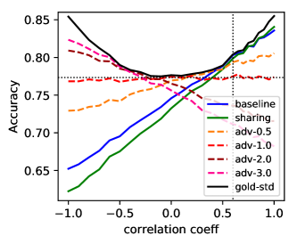
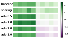
Figure 2: Synthetic experiments analysis: (a) Probabilistic data generation to create data with target shift (b) Model accuracy on test set with varying label correlation, when model was trained on training set with correlation $0.6$ (vertical dotted lines in the diagram) (c) Model weights on features. Note that best models for $y_{p}$ and $y_{a}$ give equal positive weights to first five and last five features respectively.

Observations and Insights: Fig.2(b) illustrates the test accuracy on primary label prediction against all label correlations in test set. The performance of baseline model is monotonically affected by the change in correlation between $Y_{p}$ and $Y_{a}$. Further, we observe that the performance is less affected when the correlation increases with the same polarity. A similar observation was made by [20] in bias setting and is termed bias amplification. On the other hand, adversarial models ($adv$-$1.0$) are more invariant to various label correlations in the test set that is consequence of target shift. The choice of adversarial weight (hyper-parameter $\lambda$) is critical to the performance of the model for a given test correlation. For instance, in this setup, $\lambda$=$1.0$ is the best choice when test set is uncorrelated i.e., $\rho_{p,a}^{te}=0.0$, whereas a larger $\lambda$ is more suitable for test correlations near $-0.5$. Interestingly, the choice of $\lambda$ even causes the models to achieve higher accuracy in a target shifted test set than the training set. Fig.2(c) visualizes model weights on 10-dimensional feature vector for all models. As the $\lambda$ for adversarial models increases, we observe that the model weights for the features corresponding to the auxiliary label are reduced. Furthermore, for larger value of $\lambda$, the model assigns negative weights on features corresponding to $y_{a}$. Negative weights on last five features imply that the model has captured opposite correlation between labels even though such a correlation is not observed in training.

3.3 Grouped Adversarial Learning (gAL)

We now describe our novel grouped adversarial learning to correct the effects of target shift in attribute prediction of zero-shot learning algorithms where, typically, a large number of attributes (e.g., parts of animals or birds) are predicted for unseen classes. To reiterate, our framework leverages additional information available about the unseen classes to diminish the effects of correlation shift in their attribute predictors. However, to simply extend the aforementioned intuition requires applying adversarial learning to a large number of attributes, leading to multiple adversarial branches. To ensure tractability, we devise a measure termed $\Delta_{corr}$ to weight the adversarial arms. Further, inspired from multi task learning [44, 23, 25, 24], we take a course-grained approach and split the attributes into groups such that only inter-group correlation shift is minimized. Our approach is suitable to several ZSL algorithms that produce scores corresponding to attributes. In this work, we specifically apply gAL to three popular ZSL methods: ALE [1], DEVISE [11], and SJE [2].

3.3.1 Attribute importance with $\Delta_{corr}$

For attributes $\phi_{1}$ and $\phi_{2}$, we estimate correlation coefficient for seen classes $\rho_{s}(\phi_{1},\phi_{2})$ from labelled train set and that of test set $\rho_{u}(\phi_{1},\phi_{2})$ using class-attribute mapping. $\Delta_{corr}$ is defined as:

$$\Delta_{corr}(\phi_{1},\phi_{2})=\max\{~{}\text{sgn}(\rho_{s}(\phi_{1},\phi_{2}))~{}(\rho_{s}(\phi_{1},\phi_{2})-\rho_{u}(\phi_{1},\phi_{2})),0\}.$$ (2)

We showed in Sec. 3.2.1 and Eq. 1 that higher adversarial weight is necessary to counteract a large correlation shift. However, when there is higher correlation in test set than that in train set (with same sign), we see that adversarial learning degrades the performance. Hence, we propose an adversarial weighting scheme using $\Delta_{corr}$ such that attribute pairs with positive $\Delta_{corr}$ are permitted to be adversarial to each other with $\lambda\times\Delta_{corr}$ as adversarial weights, where $\lambda$ is the common hyperparameter across all pairs of attributes.

3.3.2 Attribute Grouping

For a given attribute predictor, we propose to retain only attributes from outside its group as adversarial branches thereby permiting the predictors of attributes of same group to share feature representation and leverage their correlations. Earlier works rely on group memberships that are based on semantic similarity of attributes [24] or human perceptions. However, in the context of target shift, we hypothesize that grouping tasks based on correlation shift may be more beneficial. Specifically, the proposed measure of correlation shift, $\Delta_{corr}$, should be low among attribute pairs in the same group and high across groups. To achieve this, we form groups by clustering attributes using spectral co-clustering [7] with $\Delta_{corr}$ as the distance measure. Nevertheless, we also report our results on semantic groups (whenever applicable) for a fair comparison.

3.3.3 Model Architecture

Given group memberships of attributes and the weighting scheme, we propose a one-vs-all architecture for label prediction, with every group jointly predicting the member attributes constrained by all other groups as adversarial branches. Let $L$ denote number of groups attributes were split into. In the model, first we have feature extractors $h_{1},h_{2},\ldots,h_{L}$, which projects input instances $x$ to $L$ latent representations, each corresponding to a group. Further, to each feature extractor $h_{i}$, we connect one primary branch $f_{ii}$ which maps to attributes of group $i$ and $(L-1)$ adversarial branches $f_{ij}:j\neq i$ which maps to attributes of group $j$. $f_{ij}(h_{i}(x))\in\mathbb{R}^{d_{j}}$, provides scores for each attribute in group $j$. So, a model with $L$ groups would have a total of $L$ primary arms and $L(L-1)$ adversarial arms. The primary arm of the group latent representation is responsible for predicting all the group attributes, thus enabling sharing. During backpropagation, each latent representation is updated from the primary arm and adversarially updated from the remaining $(L-1)$ adversarial arms. The objective function for gAL is,

$$\min_{f_{ii},h_{i}}\max\limits_{\begin{subarray}{c}f_{ij}\\ i\neq j\end{subarray}}~{}~{}{{\sum}}_{k=1}^{N}~{}\Bigg{[}~{} \ell_{ZSL}([f_{11}(h_{i}(x_{k})),\ldots,f_{LL}(h_{L}(x_{k}))],\Phi^{s},y_{k})$$

$$-\lambda~{}\sum_{i=1}^{L}\sum_{\begin{subarray}{c}j=1\\ j\neq i\end{subarray}}^{L}~{}\Delta_{ij}~{}~{}\ell_{adv}(f_{ij}(h_{i}(x_{k})),\phi_{j}(x_{k}))\Bigg{]},$$ (3)

where $\ell_{ZSL}$ is the loss function of any ZSL method which takes in score vector on attributes (given in the equation as concatenation of group of attributes) and set of class-attribute vectors $\Phi$ to predict class label. $\Delta_{ij}$ is the fixed adversarial weight between groups $i$ and $j$ which is the highest pairwise $\Delta_{corr}$ between members of group $i$ and $j$ computed using Eq.2, $\lambda$ is the hyperparameter to control overall trade-off between class prediction and correcting correlation shift, and $\phi_{j}(x_{k})$ is attribute vector of group $j$ for instance $x_{k}$. $\ell_{adv}$ is a multilabel classification loss.

We can apply the gAL technique on any ZSL algorithm whose loss functions takes scores over attributes as input. We apply gAL on three popular ZSL methods in our experiments: ALE [1], DEVISE [11] and SJE [2]. In all these three methods, class score is the dot product of class-attribute vector and attribute scores (this is called linear compatibility in [49]). Score for class $c$ is computed as $\hat{y}_{c}=[f_{11}(h_{i}(x_{k})),\ldots,f_{LL}(h_{L}(x_{k}))]^{\top}\phi^{c}$. Given class prediction vector $\hat{y}(x)$ and ground truth $y(x)$, one could apply any multiclass classification loss here. DEVISE uses SVM-rank based loss, while ALE and SJE uses some extra weighting schemes over the SVM-Rank loss. We tried a fourth ZSL method of using a categorical cross-entropy loss over the class predictions denoted as softmax [50].

To optimize gAL objective function, special gradient flipping layer before the adversarial arms called gradient reversal layer [15] is used. This ensures that the model performs poorly in prediction of adversarial labels in each group, leading to decorrelated learning of attributes. For the attribute predictors in adversarial branches, there could be effects of class imbalance from the target shift, hence we choose $\ell_{adv}$ as balanced binary cross-entropy (bce) loss.

4 Experiments

4.1 Datasets and Protocol

Protocol: We follow the experimental protocol introduced in previous literature [49] for the four datasets described in Table 1. The experimental protocol is designed such that the validation set is also zero-shot in nature. We utilize the 2048-D ResNet-101 [19] feature representation and “attribute-class prior" matrices provided by the authors of [49].

Dataset	#attributes	#seen classes (train + val)	#unseen classes	#seen images (train + val)	#unseen images	$\Delta$ corr
						mean	mean @top 50%
aPY [10]	64	15+5	12	6086+1329	7924	0.073	0.145
AWA2 [49]	85	27+13	10	20218+9191	7913	0.161	0.319
CUB [47]	312	100+50	50	5875+2946	2967	0.019	0.036
SUN [51]	102	580+65	72	11600+1300	1440	0.016	0.033
aPY-CS	64	15+5	12	4299+6691	4349	0.132	0.246
AWA2-CS	85	27+13	10	22103+10383	4836	0.255	0.483
CUB-CS	312	100+50	50	5901+2958	2929	0.041	0.076
SUN-CS	102	580+65	72	11600+1300	1440	0.074	0.136

Table 1: Statistics of datasets with attribute $\Delta_{corr}$ between train and test sets.

Correlation-shift analysis and new splits: Table 1 also shows the mean difference in correlation, measured by $\Delta_{corr}$ (Eq. 2) and $\Delta_{corr}$ measured for the top $50\%$ of attribute pairs. We highlight the significantly high change in correlation for the AWA2 and aPY datasets. Further, we generate a new experimental split of train, validation and test through a greedy selection approach, termed CS split (correlation-shift split), such that the difference in correlation (measured by $\Delta_{corr}$) is maximized, while keeping the class-count per split unchanged from the existing protocol [49]. Under these CS splits, $\Delta_{corr}$ for AWA2 and aPY is even higher than before. The considerable drop in performance of baselines on these splits further highlights the problems of target shift and showcases the ability of gAL to correct for them. We skip experimentation on CUB-CS and SUN-CS as the increase in $\Delta_{corr}$ in not significant.

	Method	aPY	AWA2	CUB	SUN
$\alpha$	DAP [29]	33.8	46.1	40.0	39.9
	IAP [29]	36.6	35.9	24.0	19.4
	CONSE [34]	26.9	44.5	34.3	38.8
	CMT [41]	28.0	37.9	34.6	39.9
	SSE [58]	34.0	61.0	43.9	51.5
	LATEM [48]	35.2	55.8	49.3	55.3
	ESZSL [36]	38.3	58.6	53.9	54.5
	ALE [1]	39.7	62.5	54.9	58.1
	DEVISE [11]	39.8	59.7	52.0	56.5
	SJE [2]	32.9	61.9	53.9	53.7
	SYNC [4]	23.9	46.6	55.6	56.3
	SAE [27]	8.3	54.1	33.3	40.3
	GFZSL [46]	38.4	63.8	49.3	60.6
$\beta$	SP-AEN [6]	24.1	58.5	55.4	59.2
	f-CLSWGAN [50]	–	–	61.5	62.1
	QFZSL [43]	–	63.5	58.8	56.2
	PSR [3]	38.4	63.8	56.0	61.4
$\gamma$	ALE*	32.8	52.9	50.0	61.9
	ALE-gAL	38.3$\uparrow$ 5.5	58.2$\uparrow$5.3	52.3$\uparrow$2.3	62.2$\uparrow$0.3
	DEVISE*	33.3	57.7	44.1	55.7
	DeViSE-gAL	38.9$\uparrow$5.6	59.4$\uparrow$1.7	51.7$\uparrow$7.6	57.4$\uparrow$1.7
	SJE*	32.9	58.3	49.4	53.5
	SJE-gAL	40.5$\uparrow$7.6	62.2$\uparrow$3.9	53.2$\uparrow$3.8	60.3$\uparrow$6.8
	softmax	33.8	55.4	50.1	61.7
	softmax-gAL	40.0$\uparrow$6.2	62.1$\uparrow$6.7	52.2$\uparrow$2.1	60.8$\downarrow$0.9

Table 2: ($\alpha$) Performance reported in [49], ($\beta$) recent approaches following same settings, ($\gamma$) performance improvement with gAL on three ZSL algorithms.

4.2 Results and Discussion

The experimental results of gAL on the standard benchmark [49] and our novel correlation-shift splits are reported in tables 2 and 3 respectively. We report class-averaged top-1 accuracies for all datasets. Highest accuracies for each dataset are shown in bold and second best numbers in blue.

We first show performance of ZSL algorithms reported by [49] in Table 2:$\alpha$ for easy reference. Table 2:$\beta$ shows other recent methods reported on the same benchmarks. In the absence of available public implementations of ALE [1], SJE [2] and DeViSE [11], we use a public Python implementation whose performance is shown in Table 2:$\gamma$ (marked $*$). Also shown are the corresponding gAL variants of these algorithms, built from the same codebase (available in supplementary with detailed instructions). We also include the softmax baseline [50] trained with categorical cross-entropy loss. Except for softmax-gAL on SUN, we report substantial improvement in performance over baseline for all four datasets. The magnitudes of improvement are indicated in green. The highest improvement was observed for SJE-gAL on aPY and DeViSE-gAL on CUB, giving a boost of 7.6% over baseline.

Method	aPY-CS	AWA2-CS
ALE*	21.1	25.3
ALE-gAL	24.3$\uparrow$3.2	42.5$\uparrow$17.2
DEVISE*	19.5	33.1
DEVISE-gAL	25.7$\uparrow$6.2	38.2$\uparrow$5.1
SJE*	18.7	27.9
SJE-gAL	23.9$\uparrow$5.2	40.2$\uparrow$12.3
softmax	18.4	32.1
softmax-gAL	24.6$\uparrow$6.2	41.5$\uparrow$9.4

Table 3: Performance of gAL variants on our proposed CS splits.

The approaches corrected for correlation shift with gAL compare favourably with existing approaches on AWA2, SUN, and aPY datasets, achieving SOTA numbers on aPY (40.5%) with SJE-gAL and SUN (62.2%) with ALE-gAL. Further, gAL improves SJE on AWA2 by 3.9% to 62.2%, marginally lower than SOTA of 63.8%. The failure to achieve SOTA on CUB dataset can be attributed to the relatively low correlation shift and the hard task of predicting large number of attributes (312, largest among the 4 datasets) for class inference. However, gAL variants continue to perform better than baselines here also.

It is interesting to compare our proposed linear compatibility approach (network of linear layers with regularizers) to a non-linear compatibility based method from Table 2 such as PSR[3] or GAN-based methods like SP-AEN[6] and f-CLSWGAN[50], that generate additional data to aid training. Note that QFZSL is a transductive algorithm, and the accuracies reported here correspond to the inductive variant.

On our newly introduced CS splits, the improvement over baseline is more pronounced as shown in table 3. The highest improved is seen for ALE-gAL on AWA2-CS of 17.2%. The considerably lower accuracies of all approaches compared to Table 2 demonstrate the difficulties faced by existing ZSL algorithms in conditions of high correlation shift. Consequently, the significant improvements over baseline shows the effectiveness of gAL.

All gAL variants presented here are based on groups formed by spectral co-clustering[7] with $\Delta_{corr}$ as the distance measure (see Sec. 3.3.2). AWA2 and CUB datasets additionally provide semantic grouping of attributes that have been extensively utilized in previous literature[24]. However, we observe that the groups formed by co-clustering provide superior empirical performance (see Appendix Sec. A.1). Further, these groups continue to maintain semantic relevance. For instance, the cluster {‘lean’, ‘swims’, ‘fish’, ‘arctic’, ‘coastal’, ‘ocean’, ‘water’} clearly represents the aquatic animal classes of AWA2.

As mentioned, the adversarial weighting scheme and the choice of hyperparameter $\lambda$ are critical to gAL performance. Relevant ablations and model parameter details are also included in the supplementary material.

5 Summary

This paper shows that our grouped adversarial learning coupled with adversarial weighting strategies can be effective in curtailing target-shift in zero shot learning settings and consequently improving performance.

• Traditional zero-shot learning algorithms utilize a set of seen classes (and associated information such as attributes-class mapping) to prepare a classifier for any set of unseen classes. This paper presents a variant of zero-shot learning that utilizes additional information from specific unseen classes of attributes-class mapping to create a tailored classifier. We show that such a paradigm of zero shot learning can be useful for correcting target shift in attributes.

• By utilizing the additional information to design and weight the proposed grouped adversarial learning, we substantially improve the performance of three popular ZSL algorithms on four standard benchmark datasets, reaching SOTA on two of them.

• A functional and flexible PyTorch implementation was built for the experimental evaluation of this work along with extensive hyper-parameter tuning heuristics that are essential in training multiple adversarial arms. It has been included with the supplementary material.

6 Broader Impact

The techniques discussed in this paper broadly advance the training of zero-shot classification models, i.e., learning to classify without examples, by mitigating the effects of target-shift. We analyze the impact of our work on both aspects of machine learning with an assumption that substantial empirical improvements and resources are applied to this line of research well beyond the preliminary evaluation presented in this work.

6.1 Impact of superior zero-shot learning algorithms

The paradigm of zero-shot learning explored in this research, if matured to its full potential, equips practitioners to transition an ML model’s learning from current to new (but related) entities using only additional descriptive information. The ability to transition to new classes with such data efficiency will have transformational impact to applied areas of machine learning. For instance, a disease prediction model may adapt to a new variant with slightly different pathology using only its definition. However, machine learning for detecting or profiling may also benefit from such a model update, provided learning is done efficiently.

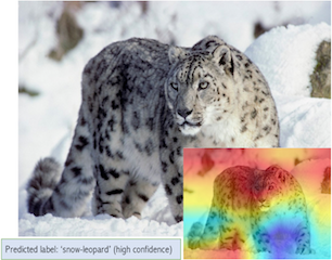
(a) typical sample

(b) typical sample

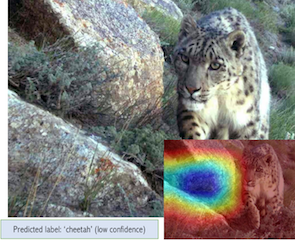
(c) rare sample

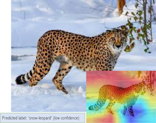
(d) rare sample

Figure 3: Visual task of classifying “cheetah vs. snow-leopard”.

6.2 Impact of panacea solution for target shift

Similarly, a near perfect solution to target shift can potentially impact generalization, transfer and domain adaptation of ML. Let us consider the visual task of classifying “cheetah vs. snow-leopard”, such as those illustrated in Fig. 3 – a task which ideally should primarily focus on the animal’s appearance. However, a large portion of these images also contain various secondary/auxiliary cues of the typical habitat of the animals in the background, i.e., tall grass and snow (see Figs 3 (a) & (b)) which are, in principle, unrelated to the animal’s appearance. An archetypal model is deceived by the co-occurrence of auxiliary cues of habitat over the animal’s primary appearance features such as complex fur patterns (see Figs 3 (c) & (d)). The poor performance of this visual classifier can be attributed to the shift in correlation between appearance and habitat labels between train and test sets. It must be noted that while the formulation of the problem is motivated in zero-shot learning, the corrosive effects of unintended correlations is a disposition of any supervised learning task from simple binary classification to recent popular supervised tasks such as object detection, captioning, or visual dialog. These and other applications of supervised learning in not only vision, but also other modalities such as speech and text, have substantial impact to our lives.

The authors readily acknowledge their limitation in foreseeing other impact of this work.

Appendix A Supplementary materials

A.1 Ablation

Results on semantic groups: As mentioned in Section 3.3, previous literature utilized a semantic grouping of attributes based on human intuition of similarity. However, we find that the cluster groups (groups formed by spectral co-clustering) via $\Delta_{corr}$ provides grouping that best minimize the chance of correlation shift. For a fair comparison, we show experiments on AWA2, CUB, and AWA2-CS performed with gAL variants based on semantic groups accompanying the datasets. These are represented by the combinations sg+Eq and sg+$\Delta_{corr}$ in Table 4. To reiterate, AWA2 comes with 10 semantic groups (e.g. nutrition, habitat) for grouping its 85 attributes whereas CUB is provided with 28 semantic groups (e.g. bill shape, wing color) for grouping its 312 attributes. The results show that cluster groups consistently outperform semantically grouped models, where available. On the challenging AWA2-CS protocol, we observe a 7% difference showcasing the importance of the proposed grouping.

Effect of adversarial weighting scheme: In Section 3.3, we present a adversarial weighting scheme such that classifier loss from the primary task is given a fixed weight of 1, while all adversarial arms are weighted proportional to $\Delta_{corr}$. Here, we present a comparison where all adversarial arms are equally weighted. These are represented by the combinations sg+Eq and cg+Eq in Table 4. An improvement of 2.5% was observed on the AWA2-CS protocol. Further, we observe a relatively stable loss in training.

Method	Group+Weights	aPY	AWA2	CUB	SUN	AWA2-CS	aPY-CS
ALE-gAL	sg+Eq	-	51.9	49.9	-	33.6	-
	sg+$\Delta_{corr}$	-	54.0	51.0	-	35.5	-
	cg+Eq	37.3	59.2	49.9	59.5	40.2	18.5
	cg+$\Delta_{corr}$	38.3	58.2	52.3	62.2	42.5	24.3
DeViSE-gAL	sg+Eq	-	51.6	48.7	-	33.2	-
	sg+$\Delta_{corr}$	-	54.9	50.1	-	34.8	-
	cg+Eq	31.9	58.2	48.7	55.6	32.6	17.5
	cg+$\Delta_{corr}$	38.9	59.4	51.7	57.4	38.2	25.7
SJE-gAL	sg+Eq	-	54.3	50.5	-	34.0	-
	sg+$\Delta_{corr}$	-	54.6	51.3	-	33.1	-
	cg+Eq	33.0	62.2	51.0	56.1	38.4	10.6
	cg+$\Delta_{corr}$	40.5	62.2	53.2	60.3	40.2	23.9
softmax-gAL	sg+Eq	-	52.9	48.5	-	35.5	-
	sg+$\Delta_{corr}$	-	54.5	49.3	-	35.4	-
	cg+Eq	37.1	61.6	50.4	59.9	40.5	14.2
	cg+$\Delta_{corr}$	40.0	62.1	52.2	60.8	41.5	24.6

Table 4: Ablations for all gAL variants with best numbers in bold, second best numbers in blue. Here, sg: semantic groups. cg:cluster groups. Eq: equal weights to all adversarial branches. $\Delta_{corr}$:weights on adversarial branches proportional to $\Delta_{corr}$. Relevant numbers from Tables 2 and 3 are shown again for easy reference.

A.2 Effect of adversarial weight $\lambda$

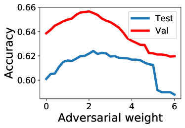
(a) SJE-gAL

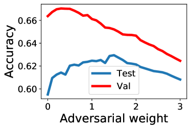
(b) softmax-gAL

Figure 4: Accuracies on AwA2 dataset with varying adversarial weight ($\lambda$) illustrates the importance of selecting the adversarial weight.

Choice of adversarial weight $\lambda$ (Eq.3.3.3) is crucial for performance of gAL models. In Fig.4, we observe how the test accuracy rises and drops as adversarial weight increases. This shows the trade-off between predicting classes and correcting correlation shift. Best value of adversarial weight is selected using validation accuracy. In Fig.4(b), the difference in performance of validation and test highlights the difficulty of finding the right value of adversarial weight.

A.3 Implementation Details

Our proposed model architecture discussed in Section 3.3.3, is illustrated in Figure 5. Following are additional details to aid reproducibility of the model architecture and training. The complete code base is provided in the supplementary material.

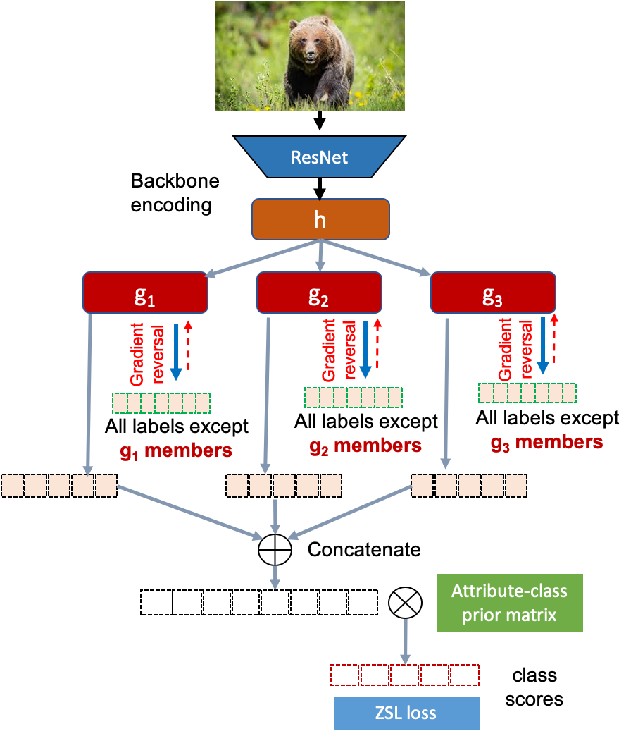
Figure 5: Proposed model architecture illustrated for 3 groups of attributes for brevity. Each group ($g_{k}$) is adversarially trained with all remaining groups. The implicit attribute scores and the class-attribute mapping is used to determine the class prediction loss.

• The best number of groups formed by spectral co-clustering (between 3 and 10) is found empirically per dataset and per classifier.

• For building our proposed gAL architecture, we first attach 500 linear layers to the input Res101 features. Next, we add another 100 layers to form the latent group representations. These are fully connected to the primary and adversarial attribute prediction neurons. None of the internal layers use any non-linear activation function. The primary group attribute predictions are concatenated before being used as input to any of the 4 classifiers (ALE, DeViSE, SJE or softmax). The adversarial attribute predictions go through an additional sigmoid activation layer before being used to compute the adversarial group losses (balanced bce loss).

• All weights in the final classifier layers (both primary and adversarial) are penalized by L2 regularization. The internal linear layers are regularized by Dropout with dropout probabilities between 0.2 to 0.5.

• All models are optimized using SGD with nesterov momentum of 0.9. Batch size is picked from {64, 128} and learning rate from {0.01, 0.001}.

• Adversarial weight $\lambda$ and the margin for SVM-rank based losses (ALE, SJE, DeViSE) are picked from a large parameter sweep for best validation error.

• We use PyTorch 1.2.0 to implement our algorithms and run all experiments on a single Tesla K80 GPU.

References

- Akata et al. [2015a] Zeynep Akata, Florent Perronnin, Zaid Harchaoui, and Cordelia Schmid. Label-embedding for image classification. IEEE transactions on pattern analysis and machine intelligence, 38(7):1425–1438, 2015a.
- Akata et al. [2015b] Zeynep Akata, Scott Reed, Daniel Walter, Honglak Lee, and Bernt Schiele. Evaluation of output embeddings for fine-grained image classification. In Proceedings of the IEEE Conference on Computer Vision and Pattern Recognition, pages 2927–2936, 2015b.
- Annadani and Biswas [2018] Yashas Annadani and Soma Biswas. Preserving semantic relations for zero-shot learning. In Proceedings of the IEEE Conference on Computer Vision and Pattern Recognition, pages 7603–7612, 2018.
- Changpinyo et al. [2016] Soravit Changpinyo, Wei-Lun Chao, Boqing Gong, and Fei Sha. Synthesized classifiers for zero-shot learning. In Proceedings of the IEEE Conference on Computer Vision and Pattern Recognition, pages 5327–5336, 2016.
- Chao et al. [2016] Wei-Lun Chao, Soravit Changpinyo, Boqing Gong, and Fei Sha. An empirical study and analysis of generalized zero-shot learning for object recognition in the wild. In European Conference on Computer Vision, pages 52–68. Springer, 2016.
- Chen et al. [2018] Long Chen, Hanwang Zhang, Jun Xiao, Wei Liu, and Shih-Fu Chang. Zero-shot visual recognition using semantics-preserving adversarial embedding networks. In Proceedings of the IEEE Conference on Computer Vision and Pattern Recognition, pages 1043–1052, 2018.
- Dhillon [2001] Inderjit S Dhillon. Co-clustering documents and words using bipartite spectral graph partitioning. In Proceedings of the seventh ACM SIGKDD international conference on Knowledge discovery and data mining, pages 269–274. ACM, 2001.
- Edwards and Storkey [2016] Harrison Edwards and Amos Storkey. Censoring representations with an adversary. Proceedings of the International Conference on Learning Representations (ICLR), 2016.
- Elkan [2001] Charles Elkan. The foundations of cost-sensitive learning. In International joint conference on artificial intelligence, volume 17, pages 973–978. Lawrence Erlbaum Associates Ltd, 2001.
- Farhadi et al. [2009] A. Farhadi, I. Endres, D. Hoiem, and D. Forsyth. Describing objects by their attributes. In 2009 IEEE Conference on Computer Vision and Pattern Recognition, pages 1778–1785, June 2009. doi: 10.1109/CVPR.2009.5206772.
- Frome et al. [2013] Andrea Frome, Greg S Corrado, Jon Shlens, Samy Bengio, Jeff Dean, Marc’Aurelio Ranzato, and Tomas Mikolov. Devise: A deep visual-semantic embedding model. In Advances in neural information processing systems, pages 2121–2129, 2013.
- Fu et al. [2014] Yanwei Fu, Timothy M Hospedales, Tao Xiang, Zhenyong Fu, and Shaogang Gong. Transductive multi-view embedding for zero-shot recognition and annotation. In European Conference on Computer Vision, pages 584–599. Springer, 2014.
- Fu et al. [2015a] Yanwei Fu, Timothy M Hospedales, Tao Xiang, and Shaogang Gong. Transductive multi-view zero-shot learning. IEEE transactions on pattern analysis and machine intelligence, 37(11):2332–2345, 2015a.
- Fu et al. [2015b] Yanwei Fu, Timothy M Hospedales, Tao Xiang, and Shaogang Gong. Transductive multi-view zero-shot learning. IEEE transactions on pattern analysis and machine intelligence, 37(11):2332–2345, 2015b.
- Ganin and Lempitsky [2015] Yaroslav Ganin and Victor Lempitsky. Unsupervised domain adaptation by backpropagation. In International Conference on Machine Learning, pages 1180–1189, 2015.
- Ganin et al. [2016] Yaroslav Ganin, Evgeniya Ustinova, Hana Ajakan, Pascal Germain, Hugo Larochelle, François Laviolette, Mario Marchand, and Victor Lempitsky. Domain-adversarial training of neural networks. The Journal of Machine Learning Research, 17(1):2096–2030, 2016.
- Goodfellow et al. [2014] Ian Goodfellow, Jean Pouget-Abadie, Mehdi Mirza, Bing Xu, David Warde-Farley, Sherjil Ozair, Aaron Courville, and Yoshua Bengio. Generative adversarial nets. In Advances in neural information processing systems, pages 2672–2680, 2014.
- Hamm [2017] Jihun Hamm. Minimax filter: Learning to preserve privacy from inference attacks. The Journal of Machine Learning Research, 18(1):4704–4734, 2017.
- He et al. [2016] Kaiming He, Xiangyu Zhang, Shaoqing Ren, and Jian Sun. Deep residual learning for image recognition. In Proceedings of the IEEE conference on computer vision and pattern recognition, pages 770–778, 2016.
- Hendricks et al. [2018] Lisa Anne Hendricks, Kaylee Burns, Kate Saenko, Trevor Darrell, and Anna Rohrbach. Women also snowboard: Overcoming bias in captioning models. arXiv preprint arXiv:1807.00517, 2018.
- Huang et al. [2019] He Huang, Changhu Wang, Philip S Yu, and Chang-Dong Wang. Generative dual adversarial network for generalized zero-shot learning. In Proceedings of the IEEE conference on computer vision and pattern recognition, pages 801–810, 2019.
- Iwasawa et al. [2017] Yusuke Iwasawa, Kotaro Nakayama, Ikuko Yairi, and Yutaka Matsuo. Privacy issues regarding the application of dnns to activity-recognition using wearables and its countermeasures by use of adversarial training. In Proceedings of the Twenty-Sixth International Joint Conference on Artificial Intelligence, IJCAI-17, pages 1930–1936, 2017. doi: 10.24963/ijcai.2017/268. URL https://doi.org/10.24963/ijcai.2017/268.
- Jacob et al. [2009] Laurent Jacob, Jean-philippe Vert, and Francis R Bach. Clustered multi-task learning: A convex formulation. In Advances in neural information processing systems, pages 745–752, 2009.
- Jayaraman et al. [2014] Dinesh Jayaraman, Fei Sha, and Kristen Grauman. Decorrelating semantic visual attributes by resisting the urge to share. In Proceedings of the IEEE Conference on Computer Vision and Pattern Recognition, pages 1629–1636, 2014.
- Kang et al. [2011] Zhuoliang Kang, Kristen Grauman, and Fei Sha. Learning with whom to share in multi-task feature learning. In International Conference on Machine Learning, volume 2, page 4, 2011.
- Kingma and Welling [2013] Diederik P Kingma and Max Welling. Auto-encoding variational bayes. arXiv preprint arXiv:1312.6114, 2013.
- Kodirov et al. [2017] Elyor Kodirov, Tao Xiang, and Shaogang Gong. Semantic autoencoder for zero-shot learning. In Proceedings of the IEEE Conference on Computer Vision and Pattern Recognition, pages 3174–3183, 2017.
- Kumar Verma et al. [2018] Vinay Kumar Verma, Gundeep Arora, Ashish Mishra, and Piyush Rai. Generalized zero-shot learning via synthesized examples. In Proceedings of the IEEE conference on computer vision and pattern recognition, pages 4281–4289, 2018.
- Lampert et al. [2013] Christoph H Lampert, Hannes Nickisch, and Stefan Harmeling. Attribute-based classification for zero-shot visual object categorization. IEEE Transactions on Pattern Analysis and Machine Intelligence, 36(3):453–465, 2013.
- Lei Ba et al. [2015] Jimmy Lei Ba, Kevin Swersky, Sanja Fidler, et al. Predicting deep zero-shot convolutional neural networks using textual descriptions. In Proceedings of the IEEE International Conference on Computer Vision, pages 4247–4255, 2015.
- Lin et al. [2002] Yi Lin, Yoonkyung Lee, and Grace Wahba. Support vector machines for classification in nonstandard situations. Machine learning, 46(1-3):191–202, 2002.
- Lipton et al. [2018] Zachary Lipton, Yu-Xiang Wang, and Alexander Smola. Detecting and correcting for label shift with black box predictors. In International Conference on Machine Learning, pages 3128–3136, 2018.
- Liu et al. [2018] Shichen Liu, Mingsheng Long, Jianmin Wang, and Michael I Jordan. Generalized zero-shot learning with deep calibration network. In Advances in Neural Information Processing Systems, pages 2005–2015, 2018.
- Norouzi et al. [2014] Mohammad Norouzi, Tomas Mikolov, Samy Bengio, Yoram Singer, Jonathon Shlens, Andrea Frome, Greg S Corrado, and Jeffrey Dean. Zero-shot learning by convex combination of semantic embeddings. Proceedings of the International Conference on Learning Representations (ICLR), 2014.
- Palatucci et al. [2009] Mark Palatucci, Dean Pomerleau, Geoffrey E Hinton, and Tom M Mitchell. Zero-shot learning with semantic output codes. In Advances in neural information processing systems, pages 1410–1418, 2009.
- Romera-Paredes and Torr [2015] Bernardino Romera-Paredes and Philip Torr. An embarrassingly simple approach to zero-shot learning. In International Conference on Machine Learning, pages 2152–2161, 2015.
- Romera-Paredes et al. [2012] Bernardino Romera-Paredes, Andreas Argyriou, Nadia Berthouze, and Massimiliano Pontil. Exploiting unrelated tasks in multi-task learning. In International Conference on Artificial Intelligence and Statistics, pages 951–959, 2012.
- Sariyildiz and Cinbis [2019] Mert Bulent Sariyildiz and Ramazan Gokberk Cinbis. Gradient matching generative networks for zero-shot learning. In The IEEE Conference on Computer Vision and Pattern Recognition (CVPR), June 2019.
- Schonfeld et al. [2019] Edgar Schonfeld, Sayna Ebrahimi, Samarth Sinha, Trevor Darrell, and Zeynep Akata. Generalized zero-and few-shot learning via aligned variational autoencoders. In Proceedings of the IEEE Conference on Computer Vision and Pattern Recognition, pages 8247–8255, 2019.
- Shigeto et al. [2015] Yutaro Shigeto, Ikumi Suzuki, Kazuo Hara, Masashi Shimbo, and Yuji Matsumoto. Ridge regression, hubness, and zero-shot learning. In Joint European Conference on Machine Learning and Knowledge Discovery in Databases, pages 135–151. Springer, 2015.
- Socher et al. [2013a] Richard Socher, Milind Ganjoo, Christopher D Manning, and Andrew Ng. Zero-shot learning through cross-modal transfer. In Advances in neural information processing systems, pages 935–943, 2013a.
- Socher et al. [2013b] Richard Socher, Milind Ganjoo, Christopher D Manning, and Andrew Ng. Zero-shot learning through cross-modal transfer. In Advances in neural information processing systems, pages 935–943, 2013b.
- Song et al. [2018] Jie Song, Chengchao Shen, Yezhou Yang, Yang Liu, and Mingli Song. Transductive unbiased embedding for zero-shot learning. In Proceedings of the IEEE Conference on Computer Vision and Pattern Recognition, pages 1024–1033, 2018.
- Thrun and O’Sullivan [1998] Sebastian Thrun and Joseph O’Sullivan. Clustering learning tasks and the selective cross-task transfer of knowledge. In Learning to learn, pages 235–257. Springer, 1998.
- Tzeng et al. [2017] Eric Tzeng, Judy Hoffman, Kate Saenko, and Trevor Darrell. Adversarial discriminative domain adaptation. In Computer Vision and Pattern Recognition (CVPR), volume 1, page 4, 2017.
- Verma and Rai [2017] Vinay Kumar Verma and Piyush Rai. A simple exponential family framework for zero-shot learning. In Joint European Conference on Machine Learning and Knowledge Discovery in Databases, pages 792–808. Springer, 2017.
- Wah et al. [2011] C. Wah, S. Branson, P. Welinder, P. Perona, and S. Belongie. The Caltech-UCSD Birds-200-2011 Dataset. Technical Report CNS-TR-2011-001, California Institute of Technology, 2011.
- Xian et al. [2016] Yongqin Xian, Zeynep Akata, Gaurav Sharma, Quynh Nguyen, Matthias Hein, and Bernt Schiele. Latent embeddings for zero-shot classification. In Proceedings of the IEEE Conference on Computer Vision and Pattern Recognition, pages 69–77, 2016.
- Xian et al. [2018a] Yongqin Xian, Christoph H Lampert, Bernt Schiele, and Zeynep Akata. Zero-shot learning-a comprehensive evaluation of the good, the bad and the ugly. IEEE transactions on pattern analysis and machine intelligence, 2018a.
- Xian et al. [2018b] Yongqin Xian, Tobias Lorenz, Bernt Schiele, and Zeynep Akata. Feature generating networks for zero-shot learning. In Proceedings of the IEEE conference on computer vision and pattern recognition, pages 5542–5551, 2018b.
- Xiao et al. [2010] J. Xiao, J. Hays, K. A. Ehinger, A. Oliva, and A. Torralba. Sun database: Large-scale scene recognition from abbey to zoo. In 2010 IEEE Computer Society Conference on Computer Vision and Pattern Recognition, pages 3485–3492, June 2010. doi: 10.1109/CVPR.2010.5539970.
- Xie et al. [2017] Qizhe Xie, Zihang Dai, Yulun Du, Eduard Hovy, and Graham Neubig. Controllable invariance through adversarial feature learning. In Advances in Neural Information Processing Systems, pages 585–596, 2017.
- Yu and Zhou [2008] Yang Yu and Zhi-Hua Zhou. A framework for modeling positive class expansion with single snapshot. In Pacific-Asia Conference on Knowledge Discovery and Data Mining, pages 429–440. Springer, 2008.
- Zemel et al. [2013] Rich Zemel, Yu Wu, Kevin Swersky, Toni Pitassi, and Cynthia Dwork. Learning fair representations. In International Conference on Machine Learning, pages 325–333, 2013.
- Zhang et al. [2018] Brian Hu Zhang, Blake Lemoine, and Margaret Mitchell. Mitigating unwanted biases with adversarial learning. arXiv preprint arXiv:1801.07593, 2018.
- Zhang et al. [2013] Kun Zhang, Bernhard Schölkopf, Krikamol Muandet, and Zhikun Wang. Domain adaptation under target and conditional shift. In International Conference on Machine Learning, pages 819–827, 2013.
- Zhang et al. [2017] Li Zhang, Tao Xiang, and Shaogang Gong. Learning a deep embedding model for zero-shot learning. In Proceedings of the IEEE Conference on Computer Vision and Pattern Recognition, pages 2021–2030, 2017.
- Zhang and Saligrama [2015] Ziming Zhang and Venkatesh Saligrama. Zero-shot learning via semantic similarity embedding. In Proceedings of the IEEE international conference on computer vision, pages 4166–4174, 2015.
- Zhou et al. [2010] Yang Zhou, Rong Jin, and Steven Chu-Hong Hoi. Exclusive lasso for multi-task feature selection. In Proceedings of the Thirteenth International Conference on Artificial Intelligence and Statistics, pages 988–995, 2010.