Top-K Deep Video Analytics: A Probabilistic Approach

Abstract.

The impressive accuracy of deep neural networks (DNNs) has created great demands on practical analytics over video data. Although efficient and accurate, the latest video analytic systems have not supported analytics beyond selection and aggregation queries. In data analytics, Top-K is a very important analytical operation that enables analysts to focus on the most important entities. In this paper, we present Everest, the first system that supports efficient and accurate Top-K video analytics. Everest  ranks and identifies the most interesting frames/moments from videos with probabilistic guarantees. Everest is a system built with a careful synthesis of deep computer vision models, uncertain data management, and Top-K query processing. Evaluations on real-world videos and the latest Visual Road benchmark show that Everest  achieves between 14.3$\times$ to 20.6$\times$ higher efficiency than baseline approaches with high result accuracy.

1. Introduction

Cameras are ubiquitous. Billions of them are being deployed in public (e.g., at road junctions) and private (e.g., in retail stores) all over the world (Norris et al., 2004). Recent advances in deep convolutional neural networks (CNNs) have led to incredible leaps in their accuracies in many machine learning tasks, notably image and video analysis. Such developments have created great demands on practical analytics over video data (Bastani et al., [n.d.]; Kang et al., 2019; Kang et al., 2017; Poms et al., 2018; Zhang et al., 2017).

Deep CNNs can extract rich semantic (e.g., object detection (He et al., 2017), facial sentiment (Yuan et al., 2013), and 3D-depth estimation (Godard et al., 2019)) from videos. Nonetheless, CNNs are also computationally expensive to train and to serve. For example, state-of-the-art object detectors run at about 5 fps (frames per second) using GPUs (He et al., 2017). This frame-processing rate is 6 times slower than the frame rate of a typical 30-fps video. Consequently, a naive “scan-and-test” approach that invokes, say, an object detector on every frame would take 6 times the duration of a video to complete an object-related query. While we can parallelize that by, say, using multiple GPUs, the computational expense remains high regardless of parallelism. Hence, the research community has started to build systems with innovative solutions to support fast analytics over video data (Anderson et al., 2018; Bastani et al., [n.d.]; Fu et al., 2019; Hsieh et al., 2018; Jiang et al., 2018; Kang et al., 2017; Kang et al., 2019; Lu et al., 2016, 2018; Nakandala and Kumar, [n.d.]; Poms et al., 2018; Xarchakos and Koudas, 2019; Zhang et al., 2017; Zhang and Kumar, 2019).

Deep video analytics is an emerging research topic that intersects database and computer vision. It is, however, still in its infancy. For example, latest systems support only selection queries such as object selection (Kang et al., 2019; Kang et al., 2017; Hsieh et al., 2018; Anderson et al., 2018; Lu et al., 2018; Moll et al., 2020; Xu et al., 2019; Daum et al., 2020) and object-trajectory selection (Bastani et al., [n.d.]; Krishnan et al., 2019). In data analytics, Top-K is a very important analytical operation that enables analysts to focus on the most important entities in the data (Carey and Kossmann, 1997; Ilyas et al., 2008; Bruno et al., 2002; Re et al., 2007). In this paper, we present the very first system for efficient Top-K video analytics. Top-K can help rank and identify the most interesting frames/moments from videos. Example use cases include:

Property Valuation. The valuation/rent of a shop is strongly related to its peak foot traffic (Charles and Kerry, 2005). Instead of manual counting, one can use a camera to capture the pedestrian flow and use a deep object detector to identify, say, the Top-5 frames (time of the day) with the highest pedestrian counts.

Thumbnail Generation. Thumbnails are images of videos that could largely affect the click-through rate of a video (Sushmita et al., 2010). To select attractive thumbnails, a social platform can use a deep visual sentimentalizer (Yuan et al., 2013) to extract, say, the Top-10 happiest moments of a video as the thumbnails for grabbing the viewers’ attention.

Fleet Management. Fleet managers in trucking businesses analyze dashcam videos to flag dangerous driving behaviors of their truck drivers (Allen, 2020). With a deep depth estimator (Godard et al., 2019), a fleet manager can query, say, the Top-50 dashcam frames based on the distance between the truck and its front vehicle as the most dangerous tailgating moments to assess drivers’ safety awareness.

In video analytics, CNN Specialization and Approximate Query Processing (AQP) are two popular techniques for overcoming the inefficiency of the scan-and-test method (Kang et al., 2017; Anderson et al., 2018; Hsieh et al., 2018; Kang et al., 2019). With CNN specialization, a video analytic system trains a lightweight query-specific model (e.g., a model specifically for “bus” detection) using frames sampled from the video-of-interest as the training data. Since the specialized CNN is highly specific to the query instance and the video-of-interest, it is both efficient to train and to serve (but is generally less accurate). The specialized CNN is then applied to all video frames to obtain a set of candidate frames that are likely to satisfy the given query. Finally, the candidate frames are passed back to a general deep model that serves as an accurate but slow-to-run “oracle” to verify their validity. Approximate Query Processing (AQP) (Kang et al., 2019; Agarwal et al., 2013) is an orthogonal technique for fast analytics when users are willing to tolerate some statistical error. The complex interplay between deep model inference and Top-K query processing, however, creates novel challenges for CNN specialization and AQP.

First, unlike selection queries where a frame satisfies a predicate or not is independent of other frames, whether a frame is in Top-K requires score comparisons between it and others. Hence, short-circuiting selections on individual frames using specialized CNNs (e.g., (Kang et al., 2017; Hsieh et al., 2018; Anderson et al., 2018)) is insufficient to Top-K query processing that requires score comparisons. Second, AQP techniques for video analytics (e.g., (Kang et al., 2019)) estimate statistics (e.g., average number of cars) but Top-K query returns a set (of frames) instead of a statistic, which demands another notion of approximation for Top-K under the video setting. Third, video data has temporal locality and thus, Top-K queries can be frame-based or window-based. For example, one could be interested in finding the Top-K 5-second clips with the highest number of vehicles. This adds to the complexity of answering Top-K queries in video analytics.

To address these challenges, we present Everest, a system that empowers users to pose Top-K and Top-K window queries on videos based on any ranking function defined over the scores provided by deep models (e.g., sentiment scores). Since model inference results are intrinsically probabilistic, Everest treats inference score distribution as a first-class citizen so that it can offer probabilistic guarantees (e.g., guaranteeing a Top-K result has 99.99% chance of being the exact result). This design is in sharp contrast to existing video analytic systems where valuable uncertainty information is largely discarded. To illustrate, Table 1(a) shows an example output of the specialized CNN used in BlazeIt (Kang et al., 2019). The (car) count in each traffic video frame is best given in the form a probability distribution by the softmax layer of the classifier, which captures the uncertainty of the prediction. Those systems, however, process queries based on a trimmed view where all cases except the most probable one are discarded (see Table 1(b)).

Supporting Top-K analytics over videos enables rich analyses over the visual world, just as what traditional Top-K query processing has done over relational data. Beyond system design, Everest has to develop new uncertain Top-K query processing algorithms based on its novel setting. Specifically, existing Top-K uncertain query processing techniques that are most related to Everest are those that use human oracles to reduce uncertainties online while evaluating a Top-K query (Zhang et al., 2015; Chu et al., 2015). Nonetheless, they offer no probabilistic guarantees and focus on human efficiency aspects instead, e.g., the plurality of a task that is needed to improve answer accuracy with considerations of human mistakes and budget limitation (Davidson et al., 2013; Kou et al., 2017). Everest, in contrast, focuses on the scalability, probabilistic guarantees, and windowing issues.

To summarize, the paper makes the following principled contributions. System-wise, Everest is the first deep video analytics system to (i) serve Top-K queries with deep semantic at scale; (ii) connect the worlds of uncertain data management with deep visual models; and (iii) provide probabilistic query guarantees. Algorithm-wise, Everest addresses the first uncertain Top-K problem with the presence of accurate but slow-to-run machine learning oracles. We have evaluated Everest using different analytical tasks on different real-world videos as well as using the latest Visual Road benchmark (Haynes et al., 2019). Experimental results show that Everest can achieve 14.3$\times$ to 20.6$\times$ speedup over different baseline approaches with high accuracy.

The remainder of this paper is organized as follows. Section 2 provides essential background and related works of this paper. Section 3 discusses Everest in detail. Section 4 gives the evaluation results. Finally, Section 5 concludes the paper.

timestamp /frame	count	prob.
$f_{1}$	0	0.78
	1	0.21
	2	0.01
$f_{2}$	0	0.49
	1	0.42
	2	0.09
$f_{3}$	0	0.16
	1	0.48
	2	0.36

(a) Output of a lightweight model

timestamp /frame	count
$f_{1}$	0
$f_{2}$	0
$f_{3}$	1

(b) Existing systems discard uncertainty information

Table 1. State-of-the-art

2. Background and Related Work

Everest builds upon research in modern video analytics and uncertain data management. In this section, we provide essential background as well as a discussion on the related works.

Traditional Visual Data Management Systems. Pioneered by Chabot (Ogle and Stonebraker, 1995) and QBIC (Flickner et al., 1995), traditional visual data management systems feature “content-based” retrieval that takes as input an example image, a sketch or a textural description of rough appearance, and outputs similar images or video segments (Potluri and Rao, 2018; Carson et al., 1997; Cascia and Ardizzone, 1996; Lee et al., 2005; Oh and Hua, 2000; Yoshitaka and Ichikawa, 1999; Zavrel et al., 2010). However, many of these systems are based on matching low-level features (e.g., colors). To query richer semantic, additional human annotations are often required (Bartolini et al., 2013; Aref et al., 2003). Top-K queries in these systems mostly leverage the geometric properties of the similarities to early-stop the process (Flickner et al., 1995; Bartolini et al., 2013). In contrast, Everest focuses on Top-K queries that rank frames based on scores from deep models (e.g., sentiment scores), where no such geometric properties are available.

Deep Video Analytics Systems. With the advent of convolutional neural networks (CNNs), richer semantic of the video can be extracted by machines with accuracy close to or even surpass human (He et al., 2015; Geirhos et al., 2017). For instance, object detectors can identify objects and their bounding boxes in an image (He et al., 2017; Redmon and Farhadi, 2018); visual sentimentalizers can evaluate the degree of happiness or sadness in an image (Yuan et al., 2013); and depth estimators can estimate 3D-depth from an image (Godard et al., 2019). Nonetheless, with millions of parameters in these deep CNNs, their high inference costs pose great challenges to modern video analytics research (Kang et al., 2017; Hsieh et al., 2018; Poms et al., 2018; Anderson et al., 2018; Zhang et al., 2017; Kang et al., 2019; Moll et al., 2020).

For analytical processing, video data is often modeled as relations, which captures the extracted semantics of the video. Table 2 shows an example of the video relation model used in BlazeIt (Kang et al., 2019), which is populated by an object detector. Specifically, each tuple in the relation corresponds to a single object in a video frame. Since a frame may contain 0 or more objects (of interest), and an object may appear in multiple frames, a frame can be associated with 0 or more tuples in a relation and an object can be associated with multiple tuples. Typical attributes of a tuple include a frame timestamp (ts), a unique id of an identified object (objectID), the object’s class label (class), bounding polygon (polygon), raw pixel content (content), and feature vector (features). To recognize identical objects across frames so that they share the same objectID, an object tracker is invoked (e.g, (Zhang et al., 2011)), which takes as input two polygons from two consecutive frames and returns the same objectID if the two polygons represent the same object. In video analytics, a video relation that is materialized by an accurate deep CNN such as YOLOv3 (Redmon and Farhadi, 2018) is regarded as the ground-truth (Hsieh et al., 2018). However, fully materializing a ground-truth relation is computationally expensive. Therefore, the key challenge is how to answer queries without fully materializing that video relation (Kang et al., 2017; Hsieh et al., 2018; Poms et al., 2018; Anderson et al., 2018; Zhang et al., 2017; Kang et al., 2019; Moll et al., 2020).

Timestamp (ts)	Class	Polygon	ObjectID	Content	Features
01-01-2019:23:05	Human	(10, 50), (30, 40), $\dots$	16	$\dots$	$\dots$
01-01-2019:23:05	Bus	(45, 58), (66, 99), $\dots$	58	$\dots$	$\dots$
01-01-2019:23:06	Human	(20, 80), (7, 55), $\dots$	16	$\dots$	$\dots$
01-01-2019:23:06	Car	(6, 91), (10, 55), $\dots$	59	$\dots$	$\dots$
01-01-2019:23:06	Car	(78, 91), (40, 55), $\dots$	60	$\dots$	$\dots$
$\dots$	$\dots$	$\dots$	$\dots$	$\dots$	$\dots$

Table 2. A video relation fully populated by a ground-truth object detector

System	Query type	Probabilistic guarantee	Window support
NoScope (Kang et al., 2017), Probabilistic predicate (Lu et al., 2018), SVQ (Xarchakos and Koudas, 2019), Focus (Hsieh et al., 2018), ExSample (Moll et al., 2020), TAHOMA (Anderson et al., 2018)	selection	✗	✗
BlazeIt (Kang et al., 2019)	selection	✗	✗
	aggregation	✓	✗
MIRIS (Bastani et al., [n.d.])	object tracking	✗	✓
Everest	Top-K	✓	✓

Table 3. Features comparisons among Everest and related deep video analytics systems

Table 3 summarizes existing video analytic systems that are most related to Everest. NoScope (Kang et al., 2017) supports object selection queries based on CNN specialization and has an optimizer to select the best model architecture (e.g., number of layers) that maximizes the throughput subject to a specified accuracy target on a validation set (but no guarantee on the whole video). BlazeIt (Kang et al., 2019) develops a SQL-like language for declarative video analytics, but it has no Top-K semantic. BlazeIt optimizes selection similar to NoScope and it also supports aggregation queries, where AQP techniques are used to bound the error. Statistical AQP techniques are inapplicable to Everest because Top-K queries returns a set (of frames) instead of a statistic. SVQ (Xarchakos and Koudas, 2019) is similar to BlazeIt with additional support to video streams and spatial constraints. “Probabilistic predicates” (Lu et al., 2018) can be viewed as a generalization of CNN specialization that allow users to express selection criteria with boolean expressions. Focus (Hsieh et al., 2018) accelerates selection by pre-building indexes for objects in videos. ExSample (Moll et al., 2020) is a sampling method to select distinct objects from videos. TAHOMA (Anderson et al., 2018) speed up object selection by transforming the input images (e.g., reducing resolution). MIRIS (Bastani et al., [n.d.]) is a system that supports object tracking (i.e., predicates that span across multiple frames). It guarantees accuracy on a validation set but not the whole video. None of the above systems address Top-K queries. Everest can guarantee accuracy on the whole video. Only Everest and MIRIS can support multi-frame analytics through windowing.

Uncertain Databases. In order to yield high-quality results, Everest regards deep models’ probabilistic inference results as first-class citizens. One common uncertain data representation is “x-tuples” (Aggarwal, 2009). An uncertain relation is a collection of x-tuples, each consists of a number of alternative outcomes that are associated with their corresponding probabilities (e.g., Table 1(a)). Together, the alternatives form a discrete probability distribution of the true outcome. Everest avoids materializing the ground-truth video relation by populating an uncertain relation using a cheap proxy to the expensive oracle that we will introduce in Section 3.2. x-tuples are assumed to be independent of each other. We will discuss later how Everest uses a difference detector so that the outputs of the proxy scorer can be represented by the x-tuple model (i.e., the inference result of a video frame is captured by one x-tuple). Hence, in the following discussion, we use the terms x-tuple, frame, and timestamp interchangeably.

Uncertain Top-K Processing. There are different notions of uncertain Top-K queries (Cormode et al., 2009; Yi et al., 2008; Soliman et al., 2008; Hua et al., 2008). The notion of U-TopK (Yi et al., 2008; Soliman et al., 2008) returns a result set that has the highest probability of being Top-K. While U-TopK may return an answer of very low probability (e.g., $10^{-6}$), Everest guarantees the answer meets a probability threshold. U-KRanks (Soliman et al., 2007, 2008) is another notion. In a U-KRanks result set, the $i$-th result in the result set is the most probable one to be ranked $i$-th. However, that does not guarantee that the result set as a whole is the most probable Top-K answer. Probabilistic threshold Top-K (Hua et al., 2008) is yet another notion. A Top-K result of such kind consists of all the tuples (can be less/more than $K$ tuples) whose individual probability of being one of the Top-K tuples is larger than a given threshold. There is no guarantee that the result set as a whole is the most probable Top-K answer. For example, it may return an empty set when no tuple satisfies the threshold requirement. The above uncertain Top-K query processing works have been assuming no ground-truth is accessible at run-time. In contrast, Everest can access an accurate but slow-to-run oracle to reduce data uncertainties online and thus achieve oracle-in-the-loop uncertain Top-K query processing.

Uncertain Top-K Processing with an Oracle. With a slow-to-run but accurate oracle accessible while processing uncertain Top-K queries, Everest is related to the topic of uncertain data cleaning (Mo et al., 2013; Cheng et al., 2008; Zhang et al., 2015). There are two branches in uncertain data cleaning. The main branch is to identify the best set of uncertain tuples for a “cleaning agent” (e.g., a human expert) to clean data offline. A human expert is served as an oracle. As employing a human expert involves monetary cost, existing works focus on minimizing the expected entropy over the set of possible query answers within a cleaning budget (e.g., the number of uncertain tuples to be sent to the cleaning agent) (Mo et al., 2013; Cheng et al., 2008). In that branch of work, the cleaning agent is technically out of the processing loop and an algorithm simply identifies the batch of uncertain tuples that have to be cleaned and terminates. In contrast, Everest puts the oracle in the loop and carries out “cleaning” online. Hence, it can provide probabilistic guarantees on the query answer, which is way more intuitive than using entropy. The other branch of work is closer to Everest because it has an online oracle-in-the-loop setting. Specifically, that direction leverages a crowdsourcing platform (e.g., Amazon Mechanical Turk) to reduce the uncertainties online while processing an uncertain Top-K query (Zhang et al., 2015). However, existing works focus more on the human efficiency issues. In contrast, Everest focuses on the scalability, probabilistic guarantees, and windowing issues.

timestamp	num of cars
$f_{1}$	0
$f_{2}$	0
$f_{3}$	0

(a)

timestamp	num of cars
$f_{1}$	1
$f_{2}$	0
$f_{3}$	0

(b)

Table 4. Two possible worlds $W_{1}$ and $W_{2}$

timestamp	num of cars	conf.
$f_{1}$	0	0.78
	1	0.21
	2	0.01
$f_{2}$	0	0.49
	1	0.42
	2	0.09
$f_{3}$	0	1.0

Table 5. After applying $\textsf{Oracle}(f_{3})$ on Table 1(a)

3. Everest

Everest allows users to set a per-query threshold, ${\tt thres}$, to ensure that the returned Top-K result has a minimum of ${\tt thres}$ probability to be the exact answer. Given an uncertain relation $D$ obtained from a video (Section 3.2 will discuss how to obtain that) and a scoring function $S$ (e.g., defining the score of a frame $f$ be the number of cars in $f$ identified by an oracle object detector), Everest returns a Top-K result $\hat{R}$ with confidence $\hat{p}=\Pr(\hat{R}=R)\geq{\tt thres}$, where $R$ is the exact result and ${\tt thres}$ is the probability threshold specified by the user. The probability $\hat{p}$ is defined over an uncertain relation $D$ (e.g., Table 1(a)) using the possible world semantic (PWS) (Moore, 1984). The possible world semantic is widely used in uncertain databases, where an uncertain relation is instantiated to multiple possible worlds, each of which is associated with a probability. Table 4 shows two possible worlds (out of $3^{3}$) of Table 1(a). Given the probability of each possible world, the confidence $\hat{p}$ of a Top-K answer $\hat{R}$ is the sum of probabilities of all possible worlds in which $\hat{R}$ is Top-K:

(1) $$\hat{p}=\sum_{W\in\mathcal{W}(D)\land\hat{R}=\text{Top-K}(W)}\Pr(W).$$

Here, $\mathcal{W}(D)$ denotes the set of all possible worlds of an uncertain relation $D$. In addition, the answer $\hat{R}$ has to satisfy the following:

DEFINITION 0.

The Certain-Result Condition: The Top-K result $\hat{R}$ has to be chosen from $D^{c}$, where frames in $D^{c}\subseteq D$ are all certain, i.e., their frame scores are obtained from the given oracle so that they have no uncertainty.

The certain-result condition is important and unique in video analytics. For instance, the Top-1 result of the uncertain relation $D$ in Table 1(a) is $\hat{R}=\{f_{3}\}$ and it has a confidence of $\hat{p}=0.85$ based on Equation 1. Assuming ${\tt thres}=0.8$, the confidence of $\hat{R}$ being the correct answer is above the user threshold.

Figure 1. System Overview

However, after all this is a probabilistic result, and so the users will feel weird if they visually inspect $f_{3}$ and actually see no cars in it. The certain-result condition avoids such awkward answers and constrains that all the tuples in $\hat{R}$ have to be confirmed by the oracle before it is returned to the users. With the certain-result condition, $\{f_{3}\}$ would not be returned as the Top-1 result because its probability of being Top-1 is only 0.38 based on the updated uncertain relation $D^{\prime}$ in Table 5, in which the exact score of $f_{3}$ is obtained from the oracle (we denote that operation as Oracle($f_{3}$)). Finally, we remark that $\hat{p}=\Pr(\hat{R}=R)\geq{\tt thres}$ guarantees not only the whole result set $\hat{R}$ has at least ${\tt thres}$ probability of being the true answer, but every frame $\hat{f}$ in $\hat{R}$ also has at least ${\tt thres}$ probability of being in the exact result set $R$ because $\Pr(\hat{f}\in R)\geq\Pr(\hat{R}=R)\geq{\tt thres}$. $\Pr(\hat{f}\in R)$ reflects the precision of Top-K answer, i.e., the fraction of results in $\hat{R}$ that belongs to $R$. Therefore, Everest effectively provides probabilistic guarantees on the precision of the query answers.

3.1. System Overview

Following recent works (Anderson et al., 2018; Hsieh et al., 2018; Kang et al., 2017), Everest also focuses on a batch setting. In this setting, large quantities of video are collected for post-analysis. Online analytics on live video stream is a different setting and is beyond the scope of this paper. To our knowledge, tracking model drift in visual data is still an ongoing research in computer vision (Kang et al., 2017). We will tackle that problem upon robust techniques for resolving model drift are developed.

Figure 1 shows a system overview. Everest leverages CNN specialization and uncertain query processing to accelerate Top-K analytics with probabilistic guarantees. Processing a query involves two phases. The first phase trains a lightweight convolutional mixture density network (CMDN) (D’Isanto and Polsterer, 2017) that outputs a rough score distribution for each frame to form an initial uncertain relation $D_{0}$ quickly. The second phase takes as input the resulting uncertain relation $D_{0}$ from Phase 1 and finds a Top-K result $\hat{R}$ that has a confidence $\hat{p}\geq{\tt thres}$. Initially, given $D_{0}$ only, it is unlikely that the initial Top-K result $\hat{R}_{0}$ from $D_{0}$ gives a confidence that is above the threshold. Furthermore, given a potential Top-K result $\hat{R}$, we have to confirm its frames for the certain-result condition using the oracle — but that may conversely give the same $\hat{R}$ a lower confidence based on the updated uncertain relation $D^{\prime}$ (e.g., drops from 0.85 to 0.38). Of course, if the uncertain relation $D^{\prime}$ contains no more uncertainty (i.e., all tuples are certain), the Top-K result from that $D^{\prime}$ has a confidence of 1. Consequently, Phase 2 can be viewed as Top-K processing via online uncertain data cleaning, in which the system selectively “cleans” the uncertain tuples in the uncertain relation using the oracle until the Top-K result from the latest uncertain relation satisfies the probabilistic guarantee. For high efficiency, Phase 2 aims to clean as few uncertain tuples as possible because each cleaning operation invokes the computationally expensive oracle. Furthermore, the algorithms in Phase 2 have to be carefully designed because uncertain query processing often introduces an exponential number of possible worlds.

3.2. Phase 1: Building the initial uncertain relation $D_{0}$ using convolutional mixture density network (CMDN)

The crux of CNN specialization is to design a fast but less accurate proxy model to approximate the functionality of the original accurate but slow-running oracle model (e.g., a less accurate but fast running object detector). Since users in Everest can specify different scoring (ranking) functions by providing any deep model as the oracle (e.g., sentimentalizer, depth estimator) at run-time, it is impossible for Everest to prepare the proxy models ahead. In view of this, we decide to build a proxy scorer that can approximate any score distribution instead of building a proxy that approximates an oracle’s original functionality. In order to approximate any arbitrary scoring function and predicting the probability density of a frame’s estimated score (instead of a point-estimate), we train a convolutional mixture density network (CMDN) to approximate the score distribution. With that, the training data is obtained by randomly sampling frames from the video-of-interest and obtaining their exact scores through invoking the accurate oracle.

Figure 2 shows the CMDN we designed. It uses five convolution layers to extract features from the input frame, where the $i$-th layer has $2^{i+3}$ filters of $3\times 3$ kernel, followed by a $2\times 2$ max-pooling. Finally the extracted features are fed to a mixed density network (with $h$ hypothesis) to output parameters of $g$ Gaussians (each has a mean $\mu$ and variance $\sigma$) and their weights $\pi$ in the mixture.

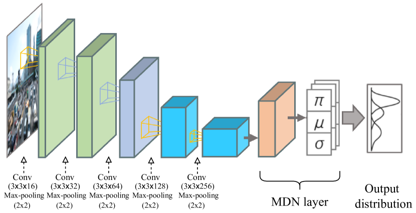
Figure 2. Everest uses a Convolutional Mixture Density Network as a proxy scorer

In order to generate robust models, we train multiple CMDN models with different sets of hyperparameters (e.g., $h$ and $g$). Since both the model and the training data are small, the total training time is less than several minutes. After training, Everest selects the best model by evaluating the models on a holdout set. The holdout set is obtained the same way as the training samples. The model with the smallest negative log-likelihood (NLL) (Giri and Bai, 2010) is chosen and the rest are discarded.

Before building the uncertain relation using the chosen CMDN, Everest uses a difference detector to discard similar frames from the video. This step serves two purposes. First, frames with little differences are not informative. Second, it approximates independence among frames so as to enable the use of “x-tuples” to model the data. After that, Everest feeds the unique frames to the CMDN to obtain their score distributions. An x-tuple captures a discrete distribution but the Gaussian mixture is continuous and with infinitely long tails on both ends. In order to get a finite uncertain relation, we follow (Chopin, 2011) to truncate the Gaussians so that the probabilities beyond $3\sigma$ are set to zero and evenly distributed to the rest. After that, we populate the uncertain relation $D_{0}$ by quantizing the truncated mixed Gaussian distribution. For counting based scoring function, the score distribution is quantized to a discrete distribution with non-negative integer support. For others, users have to provide the quantization step size when defining the scoring function. For frames whose exact scores were obtained during the collection of training/holdout data, they are inserted into the uncertain relation straight with no uncertainty so that no work is wasted. Nevertheless, we still call that as an “uncertain relation”.

3.3. Phase 2: Top-K processing with ground-truth-in-the-loop uncertain data cleaning

Given the uncertain relation $D_{0}$ initialized in Phase 1, the second phase aims to locate a Top-K result $\hat{R}$ whose confidence $\hat{p}$ exceeds ${\tt thres}$. As mentioned, the initial $D_{0}$ populated by the CMDN is likely to contain too much uncertainty that no Top-K result obtained from it can pass the threshold. Hence, starting with $D_{0}$, the second phase (see Figure 1 (right)) iteratively selects the best frame $f^{*}$ (by the Select-candidate function) to clean using the oracle. This process is repeated until a Top-K result $\hat{R}_{i}$ obtained from the latest table $D_{i}$ has a confidence $\hat{p}_{i}$ (computed by the Topk-prob function) that exceeds ${\tt thres}$.

Finding a Top-K result $\hat{R}_{i}$ from the latest updated table $D_{i}$ (by the Top-K($D_{i}^{c}$) function) is straightforward because it simply extracts all the certain tuples $D_{i}^{c}$ (because of the certain-result condition) from $D_{i}$ and applies an existing Top-K algorithm (e.g., (Carey and Kossmann, 1997)) to find the Top-K as $\hat{R}_{i}$. The function Topk-prob that computes the probability $\hat{p}_{i}$ for $\hat{R}_{i}$ being the exact result and the function Select-candidate that selects the most promising frame are more challenging because they involve an exponential number of possible worlds. Unfortunately, there are no existing techniques that can use an oracle to process uncertain Top-k queries with probabilistic guarantees.

$D$	Uncertain relation
$D_{i}$	Uncertain relation at iteration $i$
$D^{c}_{i}$	Subset of $D_{i}$ whose x-tuples are all certain
$D^{u}_{i}$	Subset of $D_{i}$ whose x-tuples are all uncertain
$\hat{R}$	Approximate Top-K result
$\hat{p}$	Confidence/probability of $\hat{R}$
$\hat{R}_{i},\hat{p}_{i}$	$\hat{R}$, $\hat{p}$ obtained in $i$-th iteration
$R$	Actual result
$f$	Frame / x-tuple
$S_{f}$	Score of $f$
${\mathbb{k}_{i}}$	The frame ranked $K$-th in $\hat{R}_{i}$
${\mathbb{p}_{i}}$	The frame ranked penultimately in $\hat{R}_{i}$

Table 6. Major Notations

In the following, we discuss efficient algorithms to implement the Topk-prob and the Select-candidate functions. Table 6 gives a summary of the major notations used.

3.3.1. Topk-prob($D_{i}$, $\hat{R}_{i}$)

Given a potential result $\hat{R}_{i}$ extracted from $D_{i}^{c}$, computing its confidence $\hat{p}_{i}$ via Equation 1 has to expand all $O(m^{n})$ possible worlds, where $n$ is the number of frames in $D$ and assume each of them has $m$ possible scores in the uncertain relation. However, given the certain-result condition, we can simplify the calculation of $\hat{p}_{i}$ as:

(2) $$\hat{p}_{i}=\prod_{f\in D_{i}^{u}}\Pr(S_{f}\leq S_{{\mathbb{k}_{i}}})$$

where (a) $S$ stands for the score of a frame, (b) ${\mathbb{k}_{i}}$ is the “threshold” frame that ranks $K$-th in $\hat{R}_{i}$, and its score $S_{\mathbb{k}_{i}}$ is known and certain (because ${\mathbb{k}_{i}}$ is from $\hat{R}_{i}\subseteq D_{i}^{c}$), and (c) $D_{i}^{u}$ are frames in $D_{i}$ with uncertainty, i.e., $D_{i}^{u}=D_{i}\setminus D^{c}_{i}$.

Computing Equation 2 requires only time that is linear to $|D_{i}^{u}|$. Equations 1 and 2 are equivalent because the probability of $\hat{R}_{i}$ being Top-K is equal to the probability that no frames in $D_{i}^{u}$ having scores larger than the frames in $\hat{R}_{i}$.

A further optimization is to compute two functions before Phase 2 begins: (a) the CDF $F$ for the score of each frame $f$, i.e., $F_{f}(t)=\Pr(S_{f}\leq t)=\sum\limits_{j=0}^{t}\Pr(S_{f}=t)$ and (b) a function $H(t)=\prod_{f\in D_{0}^{u}}F_{f}(t)$, which is the joint CDF of all uncertain frames in $D_{0}$. With them, in the $i$-th iteration, we can compute $\hat{p}_{i}$ as follows:

(3) $$\hat{p}_{i}=\frac{H(S_{{\mathbb{k}_{i}}})}{\prod_{f\in D_{i}^{c}}F_{f}(S_{{\mathbb{k}_{i}}})}$$

Equations 2 and 3 are equivalent because by definition $D_{i}^{u}=D_{0}^{u}\setminus D_{i}^{c}$. $F_{f}(t)$ and $H(t)$ for all $f$ and $t$ can be easily pre-computed one-off at a cost of $O(|D_{0}^{u}|)$. With Equation 3, Topk-prob($D_{i}$, $\hat{R}_{i}$) in the $i$-th iteration can compute $\hat{p}_{i}$ using $O(|D_{i}^{c}|)$ time instead, where $|D_{i}^{c}|<<|D_{i}|$.

According to Equation 2, $\hat{p}_{i}$ improves exponentially with the number of frames cleaned. Therefore, we expect Phase 2 would spend more iterations to reach a small probability threshold, say, 0.5. But after that, it would take fewer iterations to reach any probability threshold beyond.

3.3.2. Select-candidate($D^{u}_{i}$)

Select-candidate($D^{u}_{i}$) is the function to select a frame $f^{*}$ from the set of uncertain frames $D^{u}_{i}$ in the $i$-th iteration to obtain the exact score using the oracle such that cleaning $f^{*}$ can maximize $\hat{p}_{i+1}$ of the next iteration; and hopefully $\hat{p}_{i+1}\geq{\tt thres}$ after that and thus Phase 2 can stop early.

Of course, $\hat{p}_{i+1}$ is unknown before we apply Oracle($f^{*}$). Therefore, we use a random variable $X_{f}$ to denote the value of $\hat{p}_{i+1}$ after a frame $f$ is cleaned. To maximize $\hat{p}_{i+1}$, we aim to find $f^{*}=\arg\max_{f\in D_{i}^{u}}E_{i}[X_{f}]$. Using $x_{f}^{s}$ to denote the value of $X_{f}$ when $S_{f}=s$, where $s$ is a particular score, $E[X_{f}]$ is thus:

(4) $$E[X_{f}]=\sum_{s}\Pr(S_{f}=s)x_{f}^{s}$$

[Efficient computation of $x_{f}^{s}$] $x_{f}^{s}$ is the probability of the result $\hat{R}_{i+1}$ being the Top-K based on $D_{i+1}$, where the x-tuple representing $f$ in $D_{i+1}$ is assumed to be cleaned and its score is $s$ and certain. Therefore, $x_{f}^{s}$ can be calculated on top of $p_{i}$ (Equation 3) by removing the uncertainty of $f$, based on how the actual score $s$ of $f$ influences the Top-K result:

(5) $$x_{f}^{s}=\left\{\begin{aligned} &\frac{H(S_{{\mathbb{k}_{i}}})}{F_{f}(S_{{\mathbb{k}_{i}}})\prod_{f^{\prime}\in D_{i}^{c}}F_{f^{\prime}}(S_{{\mathbb{k}_{i}}})}=\frac{\hat{p}_{i}}{F_{f}(S_{{\mathbb{k}_{i}}})}&&s\leq S_{{\mathbb{k}_{i}}}\\ &\frac{H(s)}{F_{f}(s)\prod_{f^{\prime}\in D_{i}^{c}}F_{f^{\prime}}(s)}&&S_{{\mathbb{k}_{i}}}<s\leq S_{{\mathbb{p}_{i}}}\\ &\frac{H(S_{{\mathbb{p}_{i}}})}{F_{f}(S_{{\mathbb{p}_{i}}})\prod_{f^{\prime}\in D_{i}^{c}}F_{f^{\prime}}(S_{{\mathbb{p}_{i}}})}&&s>S_{{\mathbb{p}_{i}}}\end{aligned}\right.$$

The idea of Equation 5 is that:

• when $s\leq S_{\mathbb{k}_{i}}$, frame $f$ is not qualified to be in Top-K; the Top-K result would not change, and the threshold score is still $S_{\mathbb{k}_{i}}$; So, discounting the uncertainty of $f$ suffices.

• when $S_{\mathbb{k}_{i}}<s\leq S_{{\mathbb{p}_{i}}}$, frame $f$ enters the Top-K and but its score is lower than the penultimate frame ${\mathbb{p}_{i}}$ in the Top-K result, i.e., the one ranks ($K-1$)-st, so frame $f$ gets the $K$-th rank; the new “threshold” score is changed to $s$;

• when $s>S_{{\mathbb{p}_{i}}}$, frame $f$ enters the Top-K with a score greater than the original penultimate frame, the new threshold frame is ${\mathbb{p}_{i}}$, the new threshold score is changed to $S_{{\mathbb{p}_{i}}}$.

Putting Equations 5 and 4 together, we get:

(6) $$\begin{split}E[X_{f}]=\hat{p}_{i}&+\sum_{s=S_{\mathbb{k}_{i}}+1}^{S_{{\mathbb{p}_{i}}}}\frac{\Pr(S_{f}=s)H(s)}{F_{f}(s)\prod_{f^{\prime}\in D_{i}^{c}}F_{f^{\prime}}(s)}\\ &+\frac{(1-F_{f}(S_{{\mathbb{p}_{i}}}))H(S_{{\mathbb{p}_{i}}})}{F_{f}(S_{{\mathbb{p}_{i}}})\prod_{f^{\prime}\in D_{i}^{c}}F_{f^{\prime}}(S_{{\mathbb{p}_{i}}})}\end{split}$$

Equation 6 greatly reduces the cost of computing $E[X_{f}]$ compared to Equation 4 because the summation sums only over the range from $(S_{\mathbb{k}_{i}}+1)$ to $S_{{\mathbb{p}_{i}}}$.

[Finding $f^{*}$ by early stopping] To find $f^{*}$ in an iteration $i$, a baseline implementation of Select-candidate($D^{u}_{i}$) has to compute $E_{i}[X_{f}]$ for every frame $f$ in $D^{u}_{i}$. It is inefficient because $D^{u}_{i}$ is large.

Fortunately, we can deduce an upper bound, $U(X_{f})$, for each $E[X_{f}]$ and process frames in descending order of $U(X_{f})$ to early stop the computation of $f^{*}$. Specifically, starting from Equation 6, we have:

$$E[X_{f}] =\hat{p}_{i} +\sum_{s=S_{\mathbb{k}_{i}}+1}^{S_{{\mathbb{p}_{i}}}}\frac{\Pr(S_{f}=s)H(s)}{F_{f}(s)\prod_{f^{\prime}\in D_{i}^{c}}F_{f^{\prime}}(s)}$$

$$+\frac{(1-F_{f}(S_{{\mathbb{p}_{i}}}))H(S_{{\mathbb{p}_{i}}})}{F_{f}(S_{{\mathbb{p}_{i}}})\prod_{f^{\prime}\in D_{i}^{c}}F_{f^{\prime}}(S_{{\mathbb{p}_{i}}})}$$

$${\color[rgb]{1,0,0}\leq}\hat{p}_{i} +\sum_{s=S_{{\mathbb{k}_{i}}}+1}^{S_{{\mathbb{p}_{i}}}}\frac{\Pr(S_{f}=s)H({\color[rgb]{1,0,0}S_{{\mathbb{p}_{i}}}})}{F_{f}({\color[rgb]{1,0,0}S_{{\mathbb{p}_{i}}}})\prod_{f^{\prime}\in D_{i}^{c}}F_{f^{\prime}}({\color[rgb]{1,0,0}S_{{\mathbb{p}_{i}}}})}$$

$$+\frac{(1-F_{f}(S_{{\mathbb{p}_{i}}}))H(S_{{\mathbb{p}_{i}}})}{F_{f}(S_{{\mathbb{p}_{i}}})\prod_{f^{\prime}\in D_{i}^{c}}F_{f^{\prime}}(S_{{\mathbb{p}_{i}}})}$$

$$=\hat{p}_{i} +\frac{(1-F_{f}(S_{\mathbb{k}_{i}}))H(S_{{\mathbb{p}_{i}}})}{F_{f}(S_{{\mathbb{p}_{i}}})\prod_{f^{\prime}\in D_{i}^{c}}F_{f^{\prime}}(S_{{\mathbb{p}_{i}}})}$$

(7) $$=\hat{p}_{i} +\gamma\psi_{i}(f)=U(X_{f})$$

where the last line factors the terms into: $\gamma=\frac{H(S_{{\mathbb{p}_{i}}})}{\prod_{f^{\prime}\in D_{i}^{c}}F_{f^{\prime}}(S_{{\mathbb{p}_{i}}})}$ and $\psi_{i}(f)=\frac{1-F_{f}(S_{\mathbb{k}_{i}})}{F_{f}(S_{{\mathbb{p}_{i}}})}$.

In the $i$-th iteration, the order of frames’ upper bound is only determined by the “sort-factor” $\psi_{i}(f)$ because the frames share the same $\hat{p}_{i}$ and $\gamma$. This suggests Select-candidate($D^{u}_{i}$) to examine the frames in the descending order of their $\psi_{i}(f)$. When it examines a frame $f^{-}$ whose $U(X_{f^{-}})$ is smaller than any examined frame $f_{seen}$’s $E[X_{f_{seen}}]$, Select-candidate($D^{u}_{i}$) would stop early and return $f^{*}$ from those that have been examined. However, since $S_{\mathbb{k}_{i}}$ (and thus $U(X_{f})$) changes with $i$, we might have to re-compute and re-sort the frames per iteration. To avoid this overhead, we further re-write Equation 7 to:

(8) $$E[X_{f}]\leq\hat{p}_{i}+\gamma\psi_{\color[rgb]{1,0,0}j}(f)$$

where $j\leq i$. The inequality still holds because $\psi_{j}(f)\leq\psi_{i}(f)$ by observing $S_{{\mathbb{k}_{j}}}\leq S_{{\mathbb{k}_{i}}}$ and $S_{{\mathbb{p}_{j}}}\leq S_{{\mathbb{p}_{i}}}$.

With Equation 8, we can simply set $j=0$ so that we only need to compute $\psi_{j}(f)$ and sort frames in the first iteration. However, to balance between tighter bounds and efficiency, in the first 100 iterations, we set $j=\left\lfloor\frac{i}{10}\right\rfloor$, i.e., we update $\psi_{j}(f)$ and sort frames every $10$ iterations. For iterations thereafter, we update $\psi_{j}(f)$ whenever $S_{{\mathbb{k}_{i}}}$ or $S_{{\mathbb{p}_{i}}}$ change. The idea is that $S_{{\mathbb{k}_{i}}}$ and $S_{{\mathbb{p}_{i}}}$ change more in early iterations but are relatively stable afterwards.

3.4. Top-K Windows

Videos are spatial-temporal in nature and thus, users may want to split a video into time windows of finite size, compute their scores, and examine the Top-K ones. For example, an urban planner may be interested in the Top-50 5-second windows, where the score of a window is the average number of cars observed in its frames.

Everest supports Top-K over tumbling windows like the example given above. Specifically, a video-of-interest is divided into consecutive non-overlapping time windows $w_{1}$, $w_{2}$,…,$w_{n}$, each of which contains $L$ frames. The score of a window $w$, denoted by $S_{w}$, is the average of the scores of the frames in it, i.e., $S_{w}=\frac{1}{L}\sum_{f\in w}S_{f}$. For Top-K-window queries, we find the Top-K windows $\hat{R}$ such that $\hat{p}=\Pr(\hat{R}=R)\geq{\tt thres}$, where $R$ is the set of true Top-K windows.

To support this type of query, Everest builds another uncertain relation whose schema is akin to Table 1(a): (window, avg(num of cars), prob). Let the $i$-th frame in $w$ be $f^{i}$. The distribution of $S_{w}$ can be calculated based on the distributions of $S_{f^{1}},S_{f^{2}},\ldots,S_{f^{L}}$. From Section 3.2, the distribution of $S_{f^{i}}$, as obtained from the CMDN, is a $g$-component Gaussian mixture with a density of:

$$\sum_{j=1}^{g}\pi_{ij}\mathcal{N}(\mu_{ij},\sigma_{ij}^{2})$$

where $\pi_{ij}$, $\mu_{ij}$, $\sigma_{ij}$ are the weight, mean and variance of the $j$-th component in the mixture distribution of $S_{f^{i}}$, respectively. Since Everest’s difference detector (Section 3.5) discards a frame $f^{i}$ if it is too similar to a retained frame $r_{t}$, the score distribution of $S_{f^{i}}$ is approximated by the distribution of $S_{r_{t}}$. Furthermore, Everest ’s difference detector effectively divides a window into $l$ segments, where the frames in the same segment are similar to the same retained frame $r_{t}$. Since the retained frames are judged by the difference detector as sufficiently dissimilar, we assume their score distributions are independent. Let $r_{1}$, $r_{2}$, …, $r_{l}$ denote the $l$ retained frames in $w$, we approximate the distribution of $S_{w}$ by

(9) $$\begin{split}S_{w}&\sim\mathcal{N}(\frac{1}{L}\sum_{t=1}^{l}|s_{t}|\bar{\mu}_{r_{t}},\frac{1}{L}\sum_{t=1}^{l}|s_{t}|\bar{\sigma}_{r_{t}}^{2})\end{split}$$

where $|s_{t}|$ denotes the size of $t$-th segment; $\bar{\mu}_{r_{t}}$ and $\bar{\sigma}_{r_{t}}$ are the mean and the total variance of $S_{r_{t}}$, respectively. Suppose $r_{t}$ is the $q$-th frame in $w$, then

$$\begin{split}\bar{\mu}_{r_{t}}&=\sum_{j=1}^{g}\pi_{qj}\mu_{qj},\\ \bar{\sigma}_{r_{t}}^{2}&=\sum_{j=1}^{g}\pi_{qj}(\sigma_{qj}^{2}+\mu_{qj}^{2}-\bar{\mu}_{r_{t}}^{2}).\\ \end{split}$$

By quantizing the distribution in Equation 9, Everest obtains an uncertain relation of x-tuples on the mean score of each tumbling window. That uncertain table is compatible with the algorithms in Phase 2. When confirming a window using the oracle (to compute the average score of a window) during Phase 2, a large window size may require cleaning a lot of frames. Therefore, we only sample some frames to verify with the oracle and compute the sample mean.

3.5. System Details and Optimizations

Everest is implemented in Python 3.7 with Numpy 1.17. Training and inference of the CMDN are implemented using PyTorch 1.4; and we use Decord 0.4 for video decoding. Currently Everest is a standalone system. One future work is to follow RAM³S (Bartolini and Patella, 2018) to implement our techniques as a software framework so that we can leverage the various big data platforms (e.g., Spark) to scale-out.

⬇

import ...

config = get_config_from_UI()

object_of_interest = config.obj

oracle = load_model("models/yolov3.pth")

def score_func(frames):

object_lists = oracle(frames, object_of_interest)

scores = [len(objects) for objects in object_lists]

return scores

Figure 3. An object counting UDF

CMDN Training. The sampled frames are resized to 128$\times$128 resolution and pixel values are normalized to the range from 0 to 1. Everest trains $4\times 3=12$ models of different hyperparameters and selects the best one with the smallest negative log-likelihood. The set of hyperparameters are $g=\{5,8,12,15\}$ and $h=\{20,30,40\}$, where $g$ is the number of Gaussians and $h$ is the number of hypotheses in the MDN layer. All models use five convolution layers because that is empirically stable across all videos and further reducing the number of convolution layers offers no additional speedup because decoding the video would become the bottleneck.

Difference Detector. Various difference detectors (e.g., (Canel et al., 2018)) can be used in Everest. In the current implementation, we follow (Kang et al., 2017) and use mean-square-error (MSE) among pixels to measure the difference between two frames. To eliminate similar consecutive frames, in principle we need to sequentially scan through the video and discard a frame if its MSE with the last retained frame is lower than a threshold. In order to parallelize this step, we split the video into clips of $c$ frames each. Each frame in a clip is compared with the middle one in the clip (i.e., the $\lfloor\frac{c}{2}\rfloor$-th) and is discarded if their MSE is lower than a threshold. The clips are then processed in parallel. Although similar frames at the boundaries of clips may be retained or two adjacent clips may be quite similar, $c$ can be adjusted to ensure these situations are rare.

Batch Inference. The Select-candidate function in Phase 2 selects the most promising frame and infers its exact score using the oracle in each iteration. However, selecting and confirming only one frame at a time might not fully utilize the abundant GPU processing power. Therefore, our implementation selects a batch of $b$ frames that have the highest expectations based on Equation 6 and carries out batch inference. The value of $b$ depends on the FLOPS and the memory bandwidth of GPU. Although the GPU is better utilized for larger $b$, setting $b$ too large may cause cleaning unnecessary frames. Therefore, we choose $b$ based on a measurement of inference latency to ensure that the latency of cleaning $b$ frames has no significant difference from cleaning one frame.

Prefetching. Deep network inference may have I/O overheads when frames are fetched from the disk to the main memory thus stalling the GPU. The baseline scan-and-test approach can alleviate that easily by prefetching the frames because it accesses them sequentially. Our Top-K algorithm, however, selects frames to clean, which is non-sequential. Fortunately, Everest can achieve high throughput by also prefetching the input frames based on the sort-order of $\psi_{j}$ in Equation 8. Therefore, batches of frames with the highest $\psi_{j}$ would be pre-fetched while the GPU is carrying out computation.

User-defined Function (UDF). Everest accepts user-defined scoring function in the form of a Python module. Each UDF follows a signature of taking images as input and returning their oracle scores as output. Figure 3 shows the default scoring function in Everest. It uses a Pytorch implementation of YOLOv3 (Redmon and Farhadi, 2018) as the oracle and the number of appearances of the query object as the score. The weights of that model are pretrained using the COCO dataset (Lin et al., 2014) with 416$\times$416 image resolution.

4. Evaluation

We performed experiments on an Intel i9-7900X server with 64GB RAM and one NVIDIA GTX1080Ti GPU. The server runs CentOS 7.0.

Queries and Datasets. Except for the last experiment that evaluates Everest’s capability of different scoring functions (Section 4.2.5), we evaluate Everest based on the Top-K object counting. The first five rows of Table 7 shows the details of the real videos used in those experiments. Among them, three of them were also used in prior work and we add two moving camera videos (Daxi-old-street and Irish-Center) collected from Youtube. The main object-of-interest varies. For example, Archie and Taipei-bus are traffic footages and so their main objects are cars. By default, K=50 and thres=0.9.

We also include synthetic datasets generated by the latest Visual Road benchmark (Haynes et al., 2019). The synthetic datasets are used in Section 4.2.4 to evaluate the impact of the number of objects that appear in the video since we cannot control the number of objects in real videos.

Video (Used in / From)	Object-of- interest	Resolution	FPS	# of frames	Length (hrs)
Object Counting (UDF) Default
Archie ((Kang et al., 2019))	car	1920$\times$1080	30	2130k	19.7
Daxi-old-street2	person	1920$\times$1080	30	8640k	80
Grand-Canal ((Kang et al., 2017; Kang et al., 2019))	boat	1920$\times$1080	60	25100k	116.2
Irish-Center3	car	1920$\times$1080	30	32401k	300
Taipei-bus ((Kang et al., 2017; Kang et al., 2019))	car	1920$\times$1080	30	32488k	300.8
Tailgating Degree (UDF) on Dashcam Videos
Dashcam-California	car	1280$\times$720	30	324k	3
Dashcam-Greenport	car	1280$\times$720	30	350k	3.2

Table 7. Dataset Characteristics

Baselines. To our best knowledge, Everest is the first system that supports Top-K queries in modern video analytics. Therefore, there are no other systems that we can directly compare Everest with. Alternatively, we considered the following baselines in addition to the naive scan-and-test approach:

• HOG (Dalal and Triggs, 2005) is a classic computer vision method that is able to count objects in video frames without using deep learning. HOG scans over hundreds of sub-regions of the input image and performs classifications on each of them using SVM with low-level features (e.g., gradients of pixels). In this baseline, we scan the video using HOG and report the Top-K frames with the highest number of object-of-interest.

• CMDN-only. In this baseline, we consider only Phase 1 of Everest and rank a frame using its mean score from its distribution produced by the CMDN.

• TinyYOLOv3-only. TinyYOLOv3 (Redmon and Farhadi, 2018) is the light version of YOLOv3 for real-time object detection. In this baseline, we scan the video using TinyYOLOv3 and look for the Top-K frames there.

• Select-and-Topk. Lastly, we consider a baseline that is based on recent systems that support selection queries (e.g., (Kang et al., 2017; Hsieh et al., 2018; Anderson et al., 2018)). Specifically, we rewrite a Top-K query as a range selection query followed by a Top-K operation. First, we issue a range query “$S_{f}\geq\lambda M$” to such a selection system to retrieve all frames $C$ with scores higher than $\lambda M$, where $M$ is the maximum score found during specialized CNN training and $\lambda\in[0,1]$. Then, $C$ is regarded as the set of candidate frames with the highest scores and the Top-$K$ in $C$ is returned as the answer. We refer to this baseline as the Select-and-Topk method. This baseline, however, is impractical because it is hard to get the value $\lambda$ right. For example, setting $\lambda$ too large may make the number of candidate frames $|C|$ smaller than $K$. On the other hand, setting $\lambda$ too small would severely increase the selection latency because it gets a bigger set of candidate frames $C$. In our implementation of “Select-and-Topk”, we choose NoScope (Kang et al., 2017) to handle the range selection operation because it is open-source. We use the default parameters of NoScope’s optimizer and set its tolerable false negative rate to 0.1 (to mimic Everest’s thres=0.9) and false positive rate to 0 (to mimic Everest’s certain-result condition). As there are two newer systems (Focus (Hsieh et al., 2018) and TAHOMA (Anderson et al., 2018)) that are similar to NoScope, we give advantages to this baseline. First, we manually calibrate $\lambda$ in each experiment and report the one that yields the largest speedup subject to precision over 0.9. Second, we exclude NoScope’s specialized CNN training time because Focus (Hsieh et al., 2018) advocates to do training/indexing offline during data ingestion rather than online query processing. Third, we count only its time spent on the oracle in order to rule out the other factors such as the speed difference of using different video decoders.

Evaluation Metrics. For each experiment, we report (a) the end-to-end query runtime (for Everest, we include everything from Phase 1 to Phase 2 and the algorithm runtime) and the speedup over the naive scan-and-test method. We also report the result quality in terms of (b) precision (the fraction of results in $\hat{R}$ that belongs to $R$), (c) rank distance (the normalized footrule distance between the ranks of the $\hat{R}$ and their true ranks in $R$), and (d) score error (the average absolute error for scores between $\hat{R}$ and $R$).

System configurations. For Everest , in Phase 1, the number of frames in training data is set to $\min\{0.5\%n,30000\}$, where $n$ is the number of frames. We cap the sample size to be 30000 because that is sufficient even for the longest video (300.8 hours) in our datasets. The size of the holdout set is 3000 frames for all the datasets. Although the MSE threshold in the difference detector can be tuned based on the speed of the moving objects or the speed of the moving camera, we are able to use a unified MSE threshold of 0.0001 and clip size of 30 for all datasets. In Phase 2, we set the batch inference size $b$ to be 8 after measuring the inference latency on our server.

	Phase 1			Phase 2
Dataset	Label sample frames by oracle	CMDN training	Populate $D_{0}$ by CMDN inference	Select- candidate	Confirm frames using orale
Archie	10.48%	35.19%	41.75%	0.16%	12.42%
Daxi-old-street	6.34%	43.48%	45.19%	0.11%	4.88%
Grand-Canal	2.27%	20.82%	65.79%	0.34%	10.79%
Irish-Center	1.81%	15.81%	79.38%	0.16%	2.84%
Taipei-bus	1.87%	17.25%	72.23%	0.41%	8.24%

(a)

Num of iterations	% of frames cleaned
2021	0.76%
3173	0.29%
19612	0.63%
6474	0.16%
18184	0.45%

(b)

Table 8. A Detailed Breakdown

(a) Speedup (log-scale)

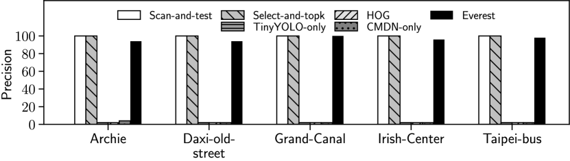
(b) Precision

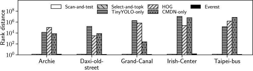
(c) Rank distance (log-scale)

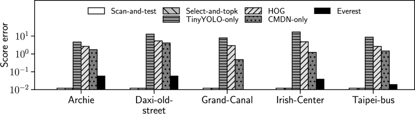
(d) Score error (log-scale)

Figure 5. Overall result under the default setting

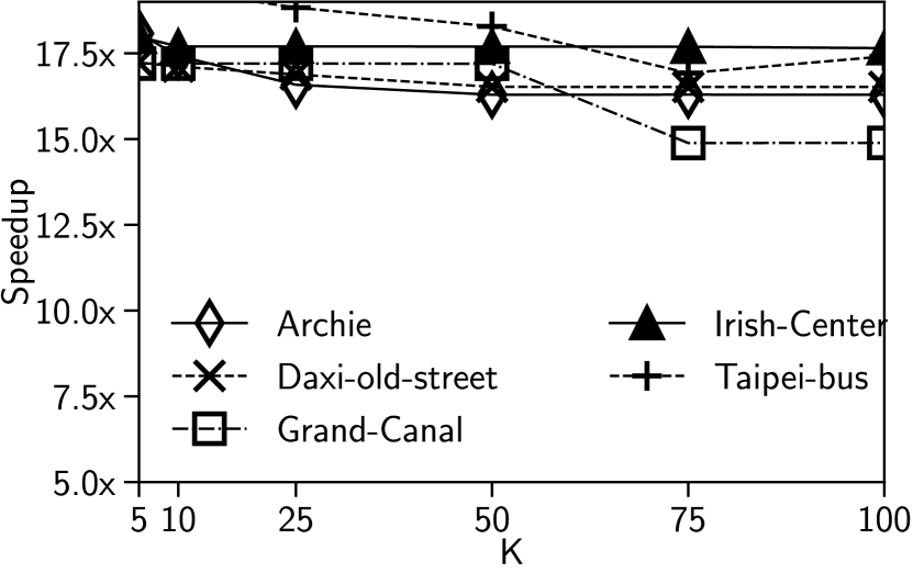
(a) Speedup

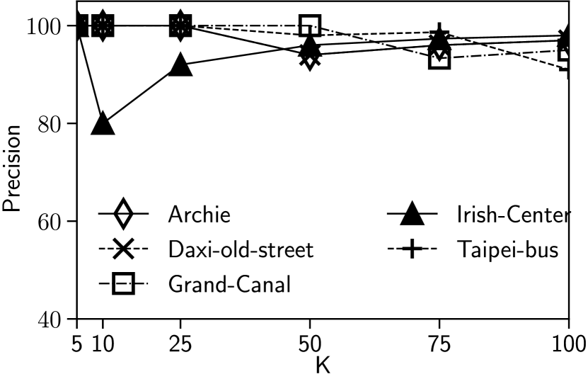
(b) Precision

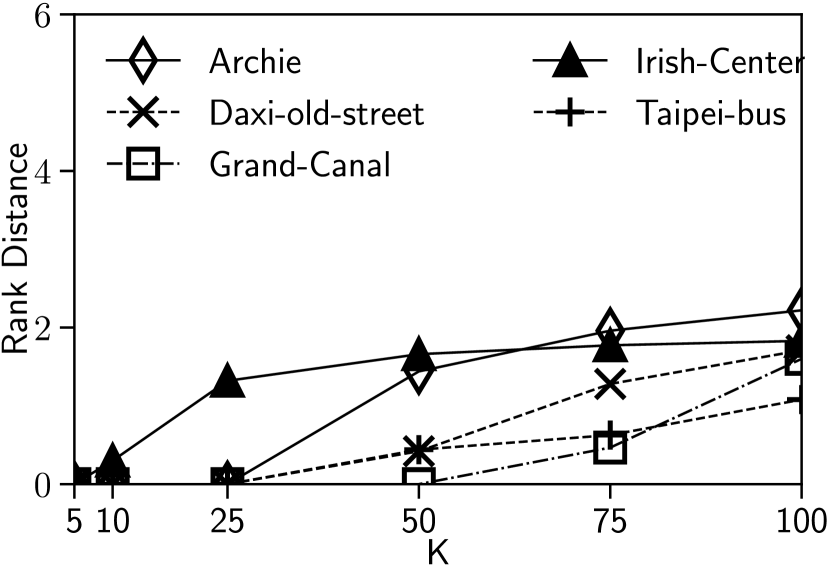
(c) Rank distance

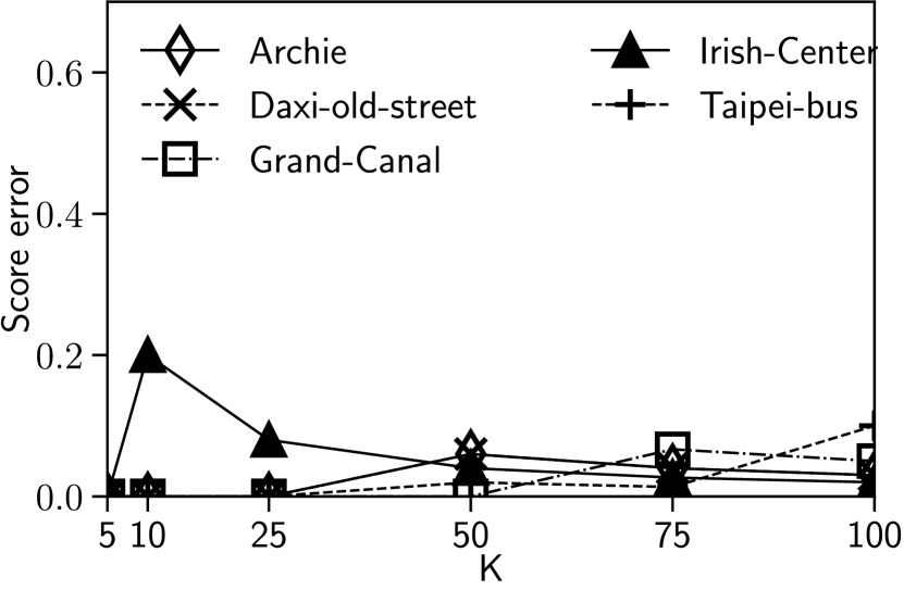
(d) Score error (log-scale)

Figure 6. Impact of K

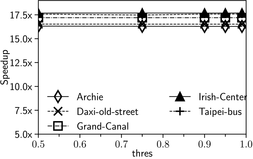
(a) Speedup

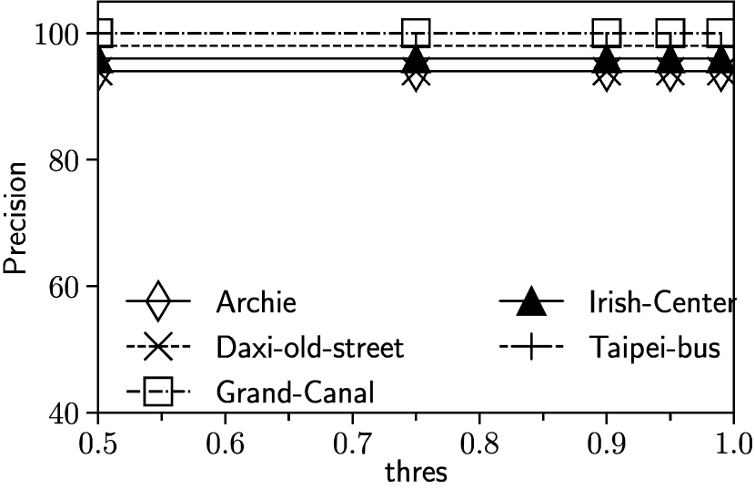
(b) Precision

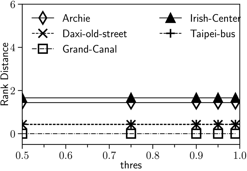
(c) Rank distance

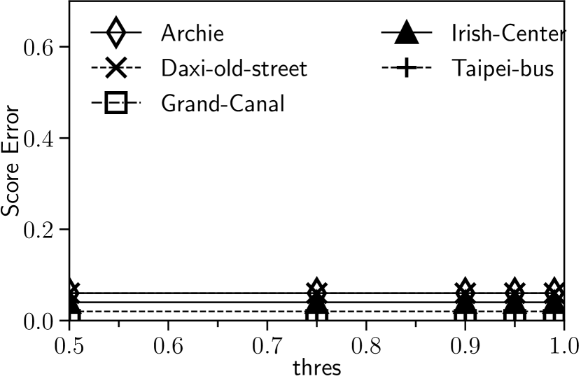
(d) Score error

Figure 7. Impact of the confidence threshold ${\tt thres}$

4.1. Overall Result and Comparisons

Our first experiment aims to give an overall evaluation of Everest. We run the default Top-50 query (thres=0.9) on five real videos. Figure 5 shows the evaluation results. The variation of the speedup on different datasets could be attributed to many factors such as the video quality as well as the distributions of the object-of-interests. Nonetheless, Everest is able to achieve a significant speedup of 16.3$\times$ to 18.3$\times$ over the scan-and-test baseline. The result quality of Everest is also excellent. Query precision values are all over 90%, which are coherent with the 0.9 probability threshold of the queries. More specifically, all queries get results of very small rank distance, which indicates that Everest returns almost perfect result with an order of speedup over the exact baseline. That can be further evidenced by observing that the score errors are all less than 0.1.

Concerning the baselines, surprisingly, HOG not only has zero to close-to-zero precision all the time, but also runs slower than Everest. The poor precision of HOG is expected because its score errors are much higher than the oracle (scan-and-test) and score errors between frames would lead to large errors in their relative rankings. Although HOG is not based on deep learning, it is slow because it requires hundreds of SVM invocations on many sub-regions per image. For CMDN-only, the experimental results indicate that CMDN could serve as the first phase of Everest, but not as a standalone system by itself. That is because running CMDN alone yields only a maximum of 1.6% precision among all datasets. TinyYOLOv3-only cannot be regarded as a true competitor neither. With so few layers used, its precision and score error are no better than HOG.

Apart from the oracle scan-and-test, select-and-topk is the only baseline that has over 0.9 precision. It has good precision because we manually tuned its $\lambda$ on each dataset. However, that precision comes with a huge cost – the experimental results show that select-and-topk is as slow as scan-and-test even though we have given it all the advantages. After we carefully look into their implementation, we found that those selection-only systems perform well on point query (e.g., finding frames that have “cars”), but not on range query (e.g., finding frames that have more than 10 cars). That result justifies the need to develop specific techniques for Top-K video analytics.

Overall, Everest is the only winner in both efficiency and accuracy. Since the non-deep method HOG and light-NN methods TinyYOLO-only and CMDN-only all yield zero to near-zero precision, we no longer include them in our further experiments below. Furthermore, since the performance of select-and-topk is similar to the oracle scan-and-test but the former requires our manual tuning and measuring advantages, we retain only the scan-and-test method as the baseline for measuring speed-up in the subsequent experiments.

4.2. Zooming into Everest

Table 8 shows a breakdown of the end-to-end query runtime of Everest. Most execution time ($\geq$80%) is spent on Phase 1 to populate the initial uncertain table because of the high volumes of frames processed by the CMDN. The cost of Phase 1 gets relatively smaller for longer videos because we cap the sample size as 30000 frames. In fact, Phase 1 can be done offline during data ingestion (e.g., Focus (Hsieh et al., 2018)) or even at the edge where the videos are produced (Hung et al., 2018). But we make no such assumption here in this paper.

Phase 2 spent most of the time confirming the frames using the oracle. Nonetheless, that is almost minimal because the fraction of frames being cleaned is very small (0.16%–0.76%). The algorithmic overheads are also minimal. In fact, the fractions of time spent executing the functions Top-K($D_{i}^{c}$) and Topk-prob($D_{i}$, $\hat{R}_{i}$) are both less than 0.01% and thus we do not show them in the table. That indicates that our algorithmic optimizations are very effective.

4.2.1. Impact of K

To understand the impact of K on Everest, we run Top-K queries using different K values: 5, 10, 25, 50, 75, and 100.

Figure 6 shows that Everest has consistently high speedup in different values of K. Generally, Everest offers slightly better speedup when K is small. That is because a smaller K results in a smaller result set, and thus the “threshold” frame tends to have a higher score (i.e., a higher $S_{{\mathbb{k}_{i}}}$). That in turns implies a higher $\hat{p}_{i}$ based on Equation 2 and so that it can stop earlier by reaching thres easier.

While the accuracy remains high for different values of K, we observe that small K values tend to influence the precision more. That is natural because the precision is a fraction influenced by the result size. For example, the precision of Everest drops below 90% on Irish-center even though Everest missed only two frames out of the Top-10 result, resulting in a 80% precision. Nonetheless, we observe that the result quality is actually high from the other two quality metrics when K is small. Therefore, if we look at the result accuracy using all three quality metrics, we can see that Everest produces high-quality results across different values of K.

4.2.2. Impact of thres

To understand the impact of the probability threshold on Everest, we run Top-50 queries using different thres values: 0.5, 0.75, 0.9, 0.95, and 0.99.

Figure 7 shows that the value of thres is not crucial as long as it is over 0.5. This is expected because we mentioned that $\hat{p}_{i}$ actually improves exponentially with the number of frames cleaned according to Equation 2. In our experiments, it took 99% of iterations to reach a probability threshold of 0.5 but only 1% of iterations to reach 0.99. This is indeed a nice result because it confirms that Everest can hide this parameter from users in real deployments.

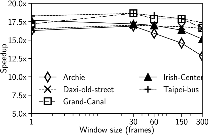
(a) Speedup

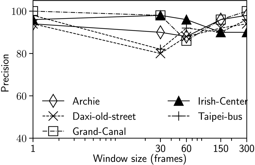
(b) Precision

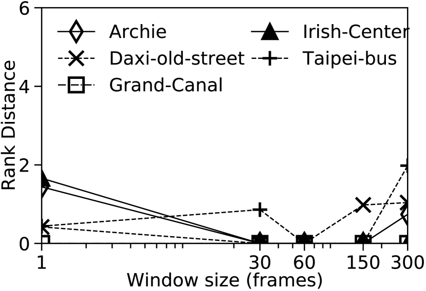
(c) Rank distance

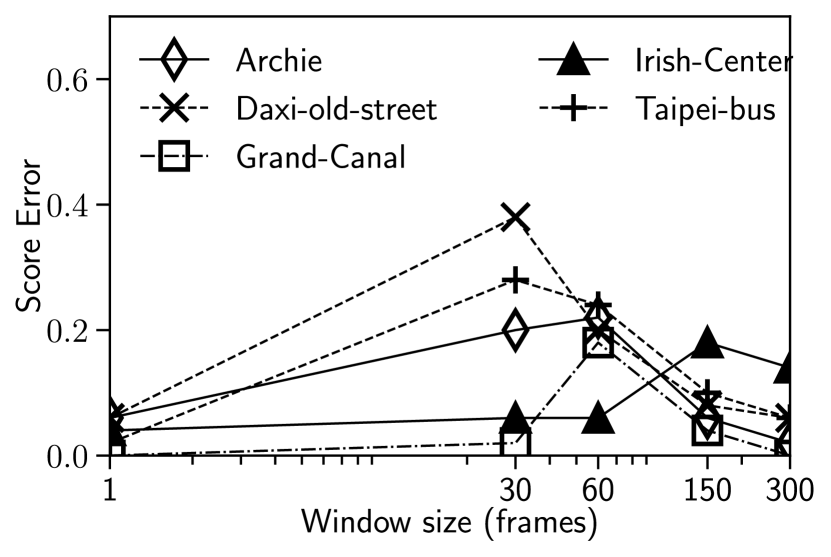
(d) Score error

Figure 8. Varying the window size

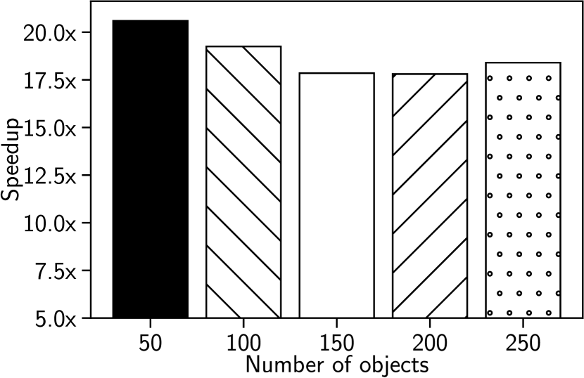
(a) Speedup

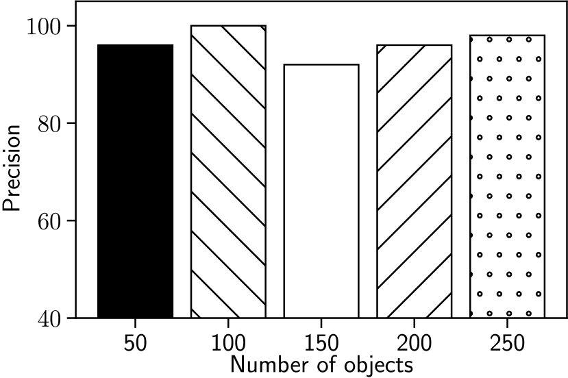
(b) Precision

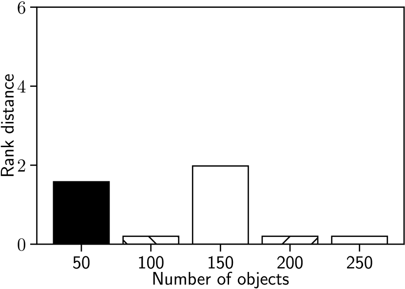
(c) Rank distance

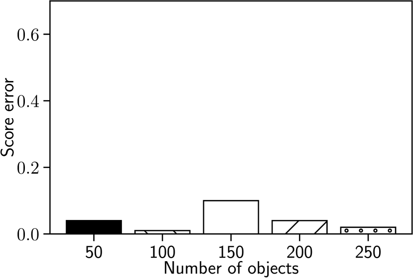
(d) Score error

Figure 9. Varying the number of objects in Visual Road

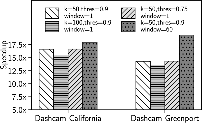
(a) Speedup

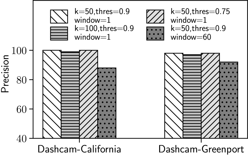
(b) Precision

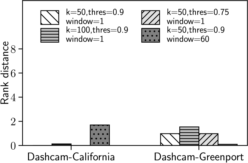
(c) Rank distance

(d) Score error

Figure 10. Scoring function using a deep depth estimator

4.2.3. Top-K Windows

To evaluate the window feature of Everest, we run Top-50 window queries with different window sizes: no window (i.e., a window of 1 frame), 30, 60, 150, and 300 frames. The probability threshold is still 0.9. In Phase 2, each window samples 10% of its frames to infer the ground-truth.

Figure 8 shows that Everest performs as good as frame-based Top-K, but the speedup drops slightly when the window size gets larger. There are two reasons. First, a larger window size essentially reduces the number of windows. As shown in the experiments above, our Top-K algorithm is smart at picking the most promising frame out of millions of frames to clean. A reduced number of windows would, however, reduce the number of choices Everest has. Second, a larger window implies more frames have to be confirmed by the oracle per selected candidate (compared with only one frame has to be confirmed per selected candidate when no window is specified).

In terms of accuracy, the result quality remains high in general. Sometimes, the precision may fluctuate a bit because of the randomness in sampling. For example, the precision of Taipei-bus drops slightly below 0.9 when the window size is 30 frames. The fluctuation diminishes when the window size gets larger because of the larger sample size.

4.2.4. Impact of Object Density

To evaluate Everest’s default object counting UDF in greater detail, we generate five 30-fps videos using the Visual Road benchmark (Haynes et al., 2019) because we cannot control that in real videos. Each generated video is ten hours long in 416$\times$416 resolution. All five synthetic videos share the same setting except the total number of cars. Specifically, the videos are all taken by the same “camera” shooting from the same “angle” of the same “mini-city”. The only moving objects in the videos are cars and we control the total number of cars in that mini-city from 50 to 250. During the data generation process, we uncovered a problem in the Visual Road benchmark in which we could only stably generate at most 15 minutes long video. After discussing with the authors of Visual Road, we concatenated 40 clips of 15-minute videos to form each ten-hour video.

Figure 9 shows the evaluation result on Visual Road under the default Top-50 query. We observe a speedup of 17.8$\times$ to 20.6$\times$ with excellent accuracy. This experiment indicates that the good performance of Everest would not be affected much by the content of the videos.

4.2.5. Scoring Function

In this last experiment, we use Everest to answer another type of query using another UDF. Specifically, we build a UDF that uses the deep depth-estimator in (Godard et al., 2019) and pose Top-K queries over two dashcam videos we found on Youtube (the last two rows in Table 2). This experiment is to recall the fleet management use case mentioned in the introduction. The objective is to find the most dangerous tailgating moments.

Figure 10 shows the results on various scenarios. These include the default Top-50 (thres=0.9) query, one Top-100 (thres=0.9) query, one Top-50 query with a smaller threshold (thres=0.75), and one Top-50 (thres=0.9) window query. We observe that Everest maintains its high result quality ($>$90% precision) with about 15$\times$ speedup over the baseline scan-and-test approach under all those different settings.

5. Conclusions and Future Work

With a massive amount of video data available and generated incessantly, the discovery of interesting information from videos becomes an exciting area of data analytics. Although deep neural networks enable semantic extraction from videos with human-level accuracy, they are unable to process video data at scale unless efficient systems are built on top. State-of-the-art video analytics systems have not supported rich analytics like Top-K. In response, we build Everest, a fast and accurate Top-K video analytics system. To our knowledge, Everest is the first video analytics system that treats the uncertain output of deep networks as a first-class citizen and provides probabilistic guaranteed accuracy. Currently, Everest is a standalone system that supports only ranking. Richer analytics can be enabled by integrating it with an expressive video query language or libraries like FrameQL (Kang et al., 2019) and Rekall (Fu et al., 2019). Finding the skyline (Bartolini et al., 2014) from such uncertain video data is also an interesting future work. Everest is an open-source project. It is available at: https://github.com/everest-project/everest.

- (1)
- Agarwal et al. (2013) Sameer Agarwal, Barzan Mozafari, Aurojit Panda, Henry Milner, Samuel Madden, and Ion Stoica. 2013. BlinkDB: queries with bounded errors and bounded response times on very large data. In Proceedings of the 8th ACM European Conference on Computer Systems. 29–42.
- Aggarwal (2009) Charu C Aggarwal. 2009. Trio a system for data uncertainty and lineage. In Managing and Mining Uncertain Data. Springer, 1–35.
- Allen (2020) James Allen. 2020. AI-powered dash cam technology gets smarter. https://www.traffictechnologytoday.com/news/incident-detection/ai-powered-dash-cam-technology-gets-smarter.html
- Anderson et al. (2018) Michael R Anderson, Michael Cafarella, Thomas F Wenisch, and German Ros. 2018. Predicate optimization for a visual analytics database. SysML (2018).
- Aref et al. (2003) Walid Aref, Moustafa Hammad, Ann Christine Catlin, Ihab Ilyas, Thanaa Ghanem, Ahmed Elmagarmid, and Mirette Marzouk. 2003. Video query processing in the VDBMS testbed for video database research. In Proceedings of the 1st ACM international workshop on Multimedia databases. 25–32.
- Bartolini et al. (2014) Ilaria Bartolini, Paolo Ciaccia, and Marco Patella. 2014. Domination in the probabilistic world: Computing skylines for arbitrary correlations and ranking semantics. ACM Transactions on Database Systems (TODS) 39, 2 (2014), 1–45.
- Bartolini and Patella (2018) Ilaria Bartolini and Marco Patella. 2018. A general framework for real-time analysis of massive multimedia streams. Multimedia Systems 24, 4 (2018), 391–406.
- Bartolini et al. (2013) Ilaria Bartolini, Marco Patella, and Corrado Romani. 2013. SHIATSU: tagging and retrieving videos without worries. Multim. Tools Appl. 63, 2 (2013), 357–385. https://doi.org/10.1007/s11042-011-0948-1
- Bastani et al. ([n.d.]) Favyen Bastani, Songtao He, Arjun Balasingam, Karthik Gopalakrishnan, Mohammad Alizadeh, Hari Balakrishnan, Michael Cafarella, Tim Kraska, and Sam Madden. [n.d.]. MIRIS: Fast Object Track Queries in Video. ([n. d.]).
- Bruno et al. (2002) Nicolas Bruno, Luis Gravano, and Amelie Marian. 2002. Evaluating top-k queries over web-accessible databases. In Proceedings 18th International Conference on Data Engineering. IEEE, 369–380.
- Canel et al. (2018) Christopher Canel, Thomas Kim, Giulio Zhou, Conglong Li, Hyeontaek Lim, David G Andersen, and SR Dulloor. 2018. Picking interesting frames in streaming video. In 2018 SysML Conference, Vol. 1. 1–3.
- Carey and Kossmann (1997) Michael J Carey and Donald Kossmann. 1997. On saying “enough already!” in sql. In Proceedings of the 1997 ACM SIGMOD international conference on Management of data. 219–230.
- Carson et al. (1997) Chad Carson, Serge Belongie, Hayit Greenspan, and Jitendra Malik. 1997. Region-based image querying. In 1997 Proceedings IEEE Workshop on Content-Based Access of Image and Video Libraries. IEEE, 42–49.
- Cascia and Ardizzone (1996) Marco La Cascia and Edoardo Ardizzone. 1996. JACOB: just a content-based query system for video databases. In 1996 IEEE International Conference on Acoustics, Speech, and Signal Processing Conference Proceedings, ICASSP ’96, Atlanta, Georgia, USA, May 7-10, 1996. IEEE Computer Society, 1216–1219. https://doi.org/10.1109/ICASSP.1996.543585
- Charles and Kerry (2005) Carter Charles and Vandell Kerry. 2005. Store location in shopping centers: Theory and estimates. Journal of Real Estate Research 27, 3 (2005), 237–266.
- Cheng et al. (2008) Reynold Cheng, Jinchuan Chen, and Xike Xie. 2008. Cleaning uncertain data with quality guarantees. Proceedings of the VLDB Endowment 1, 1 (2008), 722–735.
- Chopin (2011) Nicolas Chopin. 2011. Fast simulation of truncated Gaussian distributions. Statistics and Computing 21, 2 (2011), 275–288.
- Chu et al. (2015) Xu Chu, John Morcos, Ihab F Ilyas, Mourad Ouzzani, Paolo Papotti, Nan Tang, and Yin Ye. 2015. Katara: A data cleaning system powered by knowledge bases and crowdsourcing. In Proceedings of the 2015 ACM SIGMOD International Conference on Management of Data. 1247–1261.
- Cormode et al. (2009) Graham Cormode, Feifei Li, and Ke Yi. 2009. Semantics of ranking queries for probabilistic data and expected ranks. In 2009 IEEE 25th International Conference on Data Engineering. IEEE, 305–316.
- Dalal and Triggs (2005) Navneet Dalal and Bill Triggs. 2005. Histograms of oriented gradients for human detection. In 2005 IEEE computer society conference on computer vision and pattern recognition (CVPR’05), Vol. 1. IEEE, 886–893.
- Daum et al. (2020) Maureen Daum, Brandon Haynes, Dong He, Amrita Mazumdar, Magdalena Balazinska, and Alvin Cheung. 2020. TASM: A Tile-Based Storage Manager for Video Analytics. arXiv preprint arXiv:2006.02958 (2020).
- Davidson et al. (2013) Susan B Davidson, Sanjeev Khanna, Tova Milo, and Sudeepa Roy. 2013. Using the crowd for top-k and group-by queries. In Proceedings of the 16th International Conference on Database Theory. 225–236.
- D’Isanto and Polsterer (2017) Antonio D’Isanto and Kai Lars Polsterer. 2017. DCMDN: Deep Convolutional Mixture Density Network. Astrophysics Source Code Library (2017).
- Flickner et al. (1995) Myron Flickner, Harpreet S. Sawhney, Jonathan Ashley, Qian Huang, Byron Dom, Monika Gorkani, Jim Hafner, Denis Lee, Dragutin Petkovic, David Steele, and Peter Yanker. 1995. Query by Image and Video Content: The QBIC System. IEEE Computer 28, 9 (1995), 23–32. https://doi.org/10.1109/2.410146
- Fu et al. (2019) Daniel Y. Fu, Will Crichton, James Hong, Xinwei Yao, Haotian Zhang, Anh Truong, Avanika Narayan, Maneesh Agrawala, Christopher Ré, and Kayvon Fatahalian. 2019. Rekall: Specifying Video Events using Compositions of Spatiotemporal Labels. CoRR abs/1910.02993 (2019). arXiv:1910.02993 http://arxiv.org/abs/1910.02993
- Geirhos et al. (2017) Robert Geirhos, David HJ Janssen, Heiko H Schütt, Jonas Rauber, Matthias Bethge, and Felix A Wichmann. 2017. Comparing deep neural networks against humans: object recognition when the signal gets weaker. arXiv preprint arXiv:1706.06969 (2017).
- Giri and Bai (2010) Fouad Giri and Er-Wei Bai. 2010. Block-oriented nonlinear system identification. Vol. 1. Springer.
- Godard et al. (2019) Clément Godard, Oisin Mac Aodha, Michael Firman, and Gabriel J Brostow. 2019. Digging into self-supervised monocular depth estimation. In Proceedings of the IEEE international conference on computer vision. 3828–3838.
- Haynes et al. (2019) Brandon Haynes, Amrita Mazumdar, Magdalena Balazinska, Luis Ceze, and Alvin Cheung. 2019. Visual Road: A Video Data Management Benchmark. In Proceedings of the 2019 International Conference on Management of Data, SIGMOD Conference 2019, Amsterdam, The Netherlands, June 30 - July 5, 2019, Peter A. Boncz, Stefan Manegold, Anastasia Ailamaki, Amol Deshpande, and Tim Kraska (Eds.). ACM, 972–987. https://doi.org/10.1145/3299869.3324955
- He et al. (2017) Kaiming He, Georgia Gkioxari, Piotr Dollár, and Ross Girshick. 2017. Mask r-cnn. In Proceedings of the IEEE international conference on computer vision. 2961–2969.
- He et al. (2015) Kaiming He, Xiangyu Zhang, Shaoqing Ren, and Jian Sun. 2015. Delving deep into rectifiers: Surpassing human-level performance on imagenet classification. In Proceedings of the IEEE international conference on computer vision. 1026–1034.
- Hsieh et al. (2018) Kevin Hsieh, Ganesh Ananthanarayanan, Peter Bodik, Shivaram Venkataraman, Paramvir Bahl, Matthai Philipose, Phillip B Gibbons, and Onur Mutlu. 2018. Focus: Querying large video datasets with low latency and low cost. In 13th USENIX Symposium on Operating Systems Design and Implementation OSDI 18). 269–286.
- Hua et al. (2008) Ming Hua, Jian Pei, Wenjie Zhang, and Xuemin Lin. 2008. Ranking queries on uncertain data: a probabilistic threshold approach. In Proceedings of the 2008 ACM SIGMOD international conference on Management of data. 673–686.
- Hung et al. (2018) Chien-Chun Hung, Ganesh Ananthanarayanan, Peter Bodik, Leana Golubchik, Minlan Yu, Paramvir Bahl, and Matthai Philipose. 2018. Videoedge: Processing camera streams using hierarchical clusters. In 2018 IEEE/ACM Symposium on Edge Computing (SEC). IEEE, 115–131.
- Ilyas et al. (2008) Ihab F Ilyas, George Beskales, and Mohamed A Soliman. 2008. A survey of top-k query processing techniques in relational database systems. ACM Computing Surveys (CSUR) 40, 4 (2008), 1–58.
- Jiang et al. (2018) Junchen Jiang, Ganesh Ananthanarayanan, Peter Bodik, Siddhartha Sen, and Ion Stoica. 2018. Chameleon: scalable adaptation of video analytics. In Proceedings of the 2018 Conference of the ACM Special Interest Group on Data Communication. 253–266.
- Kang et al. (2019) Daniel Kang, Peter Bailis, and Matei Zaharia. 2019. BlazeIt: optimizing declarative aggregation and limit queries for neural network-based video analytics. Proceedings of the VLDB Endowment 13, 4 (2019), 533–546.
- Kang et al. (2017) Daniel Kang, John Emmons, Firas Abuzaid, Peter Bailis, and Matei Zaharia. 2017. NoScope: Optimizing Deep CNN-Based Queries over Video Streams at Scale. Proc. VLDB Endow. 10, 11 (2017), 1586–1597. https://doi.org/10.14778/3137628.3137664
- Kou et al. (2017) Ngai Meng Kou, Yan Li, Hao Wang, Leong Hou U, and Zhiguo Gong. 2017. Crowdsourced Top-k Queries by Confidence-Aware Pairwise Judgments. In Proceedings of the 2017 ACM International Conference on Management of Data. 1415–1430.
- Krishnan et al. (2019) Sanjay Krishnan, Adam Dziedzic, and Aaron J. Elmore. 2019. DeepLens: Towards a Visual Data Management System. In CIDR 2019, 9th Biennial Conference on Innovative Data Systems Research, Asilomar, CA, USA, January 13-16, 2019, Online Proceedings. www.cidrdb.org. http://cidrdb.org/cidr2019/papers/p40-krishnan-cidr19.pdf
- Lee et al. (2005) JeongKyu Lee, Jung-Hwan Oh, and Sae Hwang. 2005. STRG-Index: Spatio-Temporal Region Graph Indexing for Large Video Databases. In Proceedings of the ACM SIGMOD International Conference on Management of Data, Baltimore, Maryland, USA, June 14-16, 2005, Fatma Özcan (Ed.). ACM, 718–729. https://doi.org/10.1145/1066157.1066239
- Lin et al. (2014) Tsung-Yi Lin, Michael Maire, Serge Belongie, James Hays, Pietro Perona, Deva Ramanan, Piotr Dollár, and C Lawrence Zitnick. 2014. Microsoft coco: Common objects in context. In European conference on computer vision. Springer, 740–755.
- Lu et al. (2016) Yao Lu, Aakanksha Chowdhery, and Srikanth Kandula. 2016. Optasia: A relational platform for efficient large-scale video analytics. In Proceedings of the Seventh ACM Symposium on Cloud Computing. 57–70.
- Lu et al. (2018) Yao Lu, Aakanksha Chowdhery, Srikanth Kandula, and Surajit Chaudhuri. 2018. Accelerating machine learning inference with probabilistic predicates. In Proceedings of the 2018 International Conference on Management of Data. 1493–1508.
- Mo et al. (2013) Luyi Mo, Reynold Cheng, Xiang Li, David W Cheung, and Xuan S Yang. 2013. Cleaning uncertain data for top-k queries. In 2013 IEEE 29th International Conference on Data Engineering (ICDE). IEEE, 134–145.
- Moll et al. (2020) Oscar Moll, Favyen Bastani, Sam Madden, Mike Stonebraker, Vijay Gadepally, and Tim Kraska. 2020. ExSample: Efficient Searches on Video Repositories through Adaptive Sampling. arXiv preprint arXiv:2005.09141 (2020).
- Moore (1984) Robert C. Moore. 1984. Possible-World Semantics for Autoepistemic Logic. In Proceedings of the Non-Monotonic Reasoning Workshop, Mohonk Mountain House, New Paltz, NY 12561, USA, October 17-19, 1984. American Association for Artificial Intelligence (AAAI), 344–354.
- Nakandala and Kumar ([n.d.]) Supun Nakandala and Arun Kumar. [n.d.]. Vista: Declarative Feature Transfer from Deep CNNs at Scale. ([n. d.]).
- Norris et al. (2004) Clive Norris, Mike McCahill, and David Wood. 2004. The growth of CCTV: a global perspective on the international diffusion of video surveillance in publicly accessible space. Surveillance & Society 2, 2/3 (2004).
- Ogle and Stonebraker (1995) Virginia E Ogle and Michael Stonebraker. 1995. Chabot: Retrieval from a relational database of images. Computer 28, 9 (1995), 40–48.
- Oh and Hua (2000) Jung-Hwan Oh and Kien A. Hua. 2000. Efficient and Cost-effective Techniques for Browsing and Indexing Large Video Databases. In Proceedings of the 2000 ACM SIGMOD International Conference on Management of Data, May 16-18, 2000, Dallas, Texas, USA, Weidong Chen, Jeffrey F. Naughton, and Philip A. Bernstein (Eds.). ACM, 415–426. https://doi.org/10.1145/342009.335436
- Poms et al. (2018) Alex Poms, Will Crichton, Pat Hanrahan, and Kayvon Fatahalian. 2018. Scanner: Efficient video analysis at scale. ACM Transactions on Graphics (TOG) 37, 4 (2018), 1–13.
- Potluri and Rao (2018) Tejaswi Potluri and Nitta Gnaneswara Rao. 2018. Content Based Video Retrieval Using SURF, BRISK and HARRIS Features for Query-by-image. In Recent Trends in Image Processing and Pattern Recognition - Second International Conference, RTIP2R 2018, Solapur, India, December 21-22, 2018, Revised Selected Papers, Part I (Communications in Computer and Information Science, Vol. 1035), K. C. Santosh and Ravindra S. Hegadi (Eds.). Springer, 265–276. https://doi.org/10.1007/978-981-13-9181-1_24
- Re et al. (2007) Christopher Re, Nilesh Dalvi, and Dan Suciu. 2007. Efficient top-k query evaluation on probabilistic data. In 2007 IEEE 23rd International Conference on Data Engineering. IEEE, 886–895.
- Redmon and Farhadi (2018) Joseph Redmon and Ali Farhadi. 2018. Yolov3: An incremental improvement. arXiv preprint arXiv:1804.02767 (2018).
- Soliman et al. (2007) Mohamed A Soliman, Ihab F Ilyas, and Kevin Chen-Chuan Chang. 2007. Top-k query processing in uncertain databases. In 2007 IEEE 23rd International Conference on Data Engineering. IEEE, 896–905.
- Soliman et al. (2008) Mohamed A Soliman, Ihab F Ilyas, and Kevin Chen-Chuan Chang. 2008. Probabilistic top-k and ranking-aggregate queries. ACM Transactions on Database Systems (TODS) 33, 3 (2008), 1–54.
- Sushmita et al. (2010) Shanu Sushmita, Hideo Joho, Mounia Lalmas, and Robert Villa. 2010. Factors affecting click-through behavior in aggregated search interfaces. In Proceedings of the 19th ACM international conference on Information and knowledge management. 519–528.
- Xarchakos and Koudas (2019) Ioannis Xarchakos and Nick Koudas. 2019. SVQ: Streaming Video Queries. In Proceedings of the 2019 International Conference on Management of Data, SIGMOD Conference 2019, Amsterdam, The Netherlands, June 30 - July 5, 2019, Peter A. Boncz, Stefan Manegold, Anastasia Ailamaki, Amol Deshpande, and Tim Kraska (Eds.). ACM, 2013–2016. https://doi.org/10.1145/3299869.3320230
- Xu et al. (2019) Tiantu Xu, Luis Materon Botelho, and Felix Xiaozhu Lin. 2019. Vstore: A data store for analytics on large videos. In Proceedings of the Fourteenth EuroSys Conference 2019. 1–17.
- Yi et al. (2008) Ke Yi, Feifei Li, George Kollios, and Divesh Srivastava. 2008. Efficient Processing of Top-k Queries in Uncertain Databases with x-Relations. IEEE Trans. Knowl. Data Eng. 20, 12 (2008), 1669–1682. https://doi.org/10.1109/TKDE.2008.90
- Yoshitaka and Ichikawa (1999) Atsuo Yoshitaka and Tadao Ichikawa. 1999. A Survey on Content-Based Retrieval for Multimedia Databases. IEEE Trans. Knowl. Data Eng. 11, 1 (1999), 81–93. https://doi.org/10.1109/69.755617
- Yuan et al. (2013) Jianbo Yuan, Sean Mcdonough, Quanzeng You, and Jiebo Luo. 2013. Sentribute: image sentiment analysis from a mid-level perspective. In Proceedings of the Second International Workshop on Issues of Sentiment Discovery and Opinion Mining. 1–8.
- Zavrel et al. (2010) Vojtech Zavrel, Michal Batko, and Pavel Zezula. 2010. Visual video retrieval system using MPEG-7 descriptors. In Third International Workshop on Similarity Search and Applications, SISAP 2010, 18-19 September 2010, Istanbul, Turkey, Paolo Ciaccia and Marco Patella (Eds.). ACM, 125–126. https://doi.org/10.1145/1862344.1862367
- Zhang et al. (2015) Chen Jason Zhang, Lei Chen, Yongxin Tong, and Zheng Liu. 2015. Cleaning uncertain data with a noisy crowd. In 2015 IEEE 31st International Conference on Data Engineering. IEEE, 6–17.
- Zhang et al. (2017) Haoyu Zhang, Ganesh Ananthanarayanan, Peter Bodik, Matthai Philipose, Paramvir Bahl, and Michael J Freedman. 2017. Live video analytics at scale with approximation and delay-tolerance. In 14th USENIX Symposium on Networked Systems Design and Implementation (NSDI 17). 377–392.
- Zhang et al. (2011) Liyan Zhang, Ronen Vaisenberg, Sharad Mehrotra, and Dmitri V Kalashnikov. 2011. Video entity resolution: Applying er techniques for smart video surveillance. In 2011 IEEE International Conference on Pervasive Computing and Communications Workshops (PERCOM Workshops). IEEE, 26–31.
- Zhang and Kumar (2019) Yuhao Zhang and Arun Kumar. 2019. Panorama: a data system for unbounded vocabulary querying over video. Proceedings of the VLDB Endowment 13, 4 (2019), 477–491.