3D Channel Characterization and Performance Analysis of UAV-Assisted Millimeter Wave Links

Abstract

Recently, the use of millimeter wave (mmW) frequencies has emerged as a promising solution for wirelessly connecting unmanned aerial vehicles (UAVs) to ground users. However, employing UAV-assisted directional mmW links is challenging due to the random fluctuations of hovering UAVs. In this paper, the performance of UAV-based mmW links is investigated when UAVs are equipped with square array antennas. The 3GPP antenna propagation patterns are used to model the square array antenna. It is shown that the square array antenna is sensitive to both horizontal and vertical angular vibrations of UAVs. In order to explore the relationship between the vibrations of UAVs and their antenna pattern, the UAV-based mmW channels are characterized by considering the large scale path loss, small scale fading along with antenna patterns as well as the random effect of UAVs’ angular vibrations. To enable effective performance analysis, tractable and closed-form statistical channel models are derived for aerial-to-aerial (A2A), ground-to-aerial (G2A), and aerial-to-ground (A2G) channels. The accuracy of analytical models is verified by employing Monte Carlo simulations. Analytical results are then used to study the effect of antenna pattern gain under different conditions for the UAVs’ angular vibrations for establishing reliable UAV-assisted mmW links in terms of achieving minimum outage probability. Simulation results show that the performance of UAV-based mmW links with directional antennas is largely dependent on the random fluctuations of hovering UAVs. Moreover, UAVs with higher antenna directivity gains achieve better performance at larger link length. However, for UAVs with lower stability, lower antenna directivity gains result in a more reliable communication link. The developed results can therefore be applied as a benchmark for finding the optimal antenna directivity gain of UAVs under the different levels of instability without resorting to time-consuming simulations.

I Introduction

Next-generation cellular networks will inevitably rely on two technologies, high-frequency millimeter wave (mmW) bands and unmaned aerial vehicles (UAVs) [1, 2, 3, 4, 5, 6, 7, 8]. The advancement of UAV technologies and their reducing cost, have made future cellular systems more likely to be equipped with UAVs as flying base stations (BSs) which effectively enhances the network flexibility and capacity [9]. Meanwhile, flying BSs mounted on UAVs require high capacity backhaul links [10]. More recently, mmW backhauling has been proposed as a promising approach for connecting aerial BSs to a core network because of three reasons. First, unlike ground nodes that suffer from blockage, the flying nature of aerial nodes offers a higher probability of line-of-sight (LoS) between communication nodes. Second, the large available bandwidth at mmW bands can provide high capacity point-to-point aerial communication links as needed for the backhaul of aerial BSs. Third, the small wavelength enables the realization of a compact form of beam-steerable, highly directive antenna arrays on a small UAV with limited payload to compensate for the high path-loss of the mmW band [11].

To exploit the advantages of UAV equipped with directional mmW antennas, it is important to have a comprehensive and accurate channel model while taking into account the antenna propagation pattern as well as the random effect of a UAV’s angular vibrations. Although channel modeling in the context of UAV communications has been studied in recent works [12, 13, 14, 15], these studies are limited to sub-6 GHz bands which cannot be directly extended to mmW systems. Meanwhile, most of the prior studies on mmW communications [16, 17, 18] do not address the presence of UAVs, with the exception of a few recent works in [19, 20, 21, 22, 23, 24, 25, 26]. For instance, the works in [19] and [20] study a ray tracing approach to characterize the mmW propagation channel for an air-to-ground link at 28 GHz and 60 GHz under different conditions. However, the results of these works are obtained with the assumption of half-wave dipole antennas with an omni-directional pattern. The reliability and performance of UAV-based mmW links can be severely affected by impairments such as sensitivity to the atmospheric conditions and large propagation loss. Due to the UAVs’ transmission power constraints, using antennas with high gain is needed to combat severe propagation loss, particularly for longer links.

Directional UAV-based mmW communications have been the subject of more recent works such as [21] in which the authors study the directional mmW channel characteristics for UAV networks by considering the Doppler effect as a result of UAV movement. The effects of directionality and random heights in UAV-based mmW communications are studied in [22]. In [23] and [24], the authors propose an analytical framework for non-orthogonal multiple-access transmission with UAVs so as to support more users in a hotspot area such as a football stadium. In [25], the authors use stochastic geometry to study directional UAV-based backhaul links operating at 2 GHz and 73 GHz. For simplicity, in [25], the antenna pattern is approximated by a rectangular radiation pattern.

In [26], the authors study a UAV-based communication system that takes into account the dynamic blockage of mmW links. High directional mmW communication systems suffer from misalignment between transmitter (Tx) and receiver (Rx). Due to the payload limitations for employing high quality antenna stabilizers, careful alignment is not practically feasible in aerial links, particularly, for small multi-rotor UAVs. This leads to an unreliable communication system due to antenna gain mismatch between transceivers [27, 28, 29]. However, the results of these works are obtained by neglecting the effect of UAVs’ random fluctuations. More recently, the authors in [30], studied the problem of channel modeling for directional UAV-based mmW links including the effects of angle-of-arrival (AoA) and angle-of-departure (AoD) fluctuations. The results of [30] clearly demonstrate that the orientation fluctuations of hovering UAVs degrade the performance of directional UAV-based mmW links, significantly. However, the results of [30] are obtained for a simplified state of uniform linear array (ULA) of antennas. Although ULA antennas have lower complexity, the square array antenna outperforms ULA antennas.

I-A Major Contributions

The main contribution of this paper is the derivation of novel analytical channel models for UAV-based mmW links and performance analysis of UAV-based mmWave communication systems when UAVs are equipped with square array antennas. In particular, we consider balloon and rotary-wing UAVs such as quadrotor drones that can hover and remain stationary over a given area in the sky. In addition to the large scale path loss and small scale fading, we show the channel of UAV-based mmW links will be a function of UAV’s angular fluctuations along with the shape of antenna patterns. Unlike the ULA antenna that is resistant to a UAV’s horizontal fluctuations, we will show that the square array antenna is sensitive to both horizontal and vertical fluctuations, and thus, the channel characterization of UAVs equipped with square array antennas is remarkably different from ULA antenna case. In summary, our key contributions include:

• We characterize the precise channel models for three UAV-based mmW communication links: aerial-to-aerial link (called A2A link), ground-to-aerial link (called G2A link), and aerial-to-ground link (called A2G link). By taking into account the 3GPP antenna propagation patterns, the actual channel models are characterized in presence of large scale path loss and small scale fading along with the influence of UAV angular fluctuations.

• Then, for the characterized channels, we derive closed-form analytical expressions for A2A, A2G, and G2A channels. Then, by providing Monte Carlo simulations for actual UAV-based mmW channels, the accuracy of the derived analytical expressions is verified.

• We also derive the closed-form expressions for the outage probability of the considered UAV-based mmW links. The accuracy of the analytical expressions is verified by using simulations. For any given strength of UAVs’ vibrations, optimizing radiation pattern shape requires balancing an inherent tradeoff between decreasing pattern gain to alleviate the adverse effect of a UAV’s vibrations and increasing it to compensate the large path loss at mmW frequencies. The analytical results are applied as a benchmark for finding optimal antenna pattern shapes mounted on UAVs under the different levels of UAVs’ instability without resorting to time-consuming simulations.

The rest of this paper is organized as follows. In Section II, we characterize the actual channel models between UAVs. Then, in Section III, we provide the analytical channel models. Next, in Section IV, we provide the simulation results to verify the derived analytical channel models and study the link performance and antenna pattern optimization. Finally, conclusions are drawn in Section V.

II System Model

We consider a UAV-based mmW communication link that is used to provide a high capacity point-to-point link. This link can be A2A, A2G, or G2A. In an A2A link, the Tx and Rx antennas are mounted on two hovering UAVs, in an A2G link, the Tx and Rx antennas are mounted on a UAV and a ground station, respectively, and in a G2A link, the Tx and Rx antennas are mounted on a ground station and a UAV, respectively. We use the subscript $q\in\{t,r\}$ to denote respectively, the Tx and Rx antenna. For instance, let $\sigma^{2}_{qx}$ and $\sigma^{2}_{qy}$ be the standard deviations of UAV orientation fluctuations in the $x-z$ and $y-z$ axes, respectively. Thus, $\sigma^{2}_{tx}$ and $\sigma^{2}_{ty}$ represent the standard deviations of the Tx in the $x-z$ and $y-z$ axes, respectively, and $\sigma^{2}_{rx}$ and $\sigma^{2}_{ry}$ represent the standard deviations of the Rx in the $x-z$ and $y-z$ axes, respectively. In our point-to-point communication link, the UAVs are hovering in space at a distance of $Z$ from each other. The position of Tx and Rx are respectively located at $[0,0,0]$ and $[0,0,Z]$ in Cartesian coordinate system $[x,y,z]\in\mathcal{R}^{1\times 3}$ and are known at the transceiver.As shown in Fig. 1, $z$ axis refers to the direction that extends from Tx toward Rx node. The hovering UAV sets the main-lobe of array antenna pattern in the direction of $z$-axis as depicted in Fig. 1. In practice, the instantaneous orientation of a UAV can randomly deviate from its means denoted by $\theta_{q}$. This, in turn, leads to deviations in the AoD of Tx and/or AoA of Rx antenna pattern. As shown in Fig. 2, the antenna orientation fluctuations are denoted by $\theta_{qx}$ and $\theta_{qy}$ in the $x-z$ and $y-z$ Cartesian coordinates, respectively. In particular, at the Tx side, the AoD deviations are denoted by $\theta_{tx}$ and $\theta_{ty}$ in $x-z$ and $y-z$ Cartesian coordinates, respectively, and at the Rx side, the AoA deviations are denoted by $\theta_{rx}$ and $\theta_{ry}$ in $x-z$ and $y-z$ Cartesian coordinates, respectively. The UAV-based mmW links are grouped into three categories: a) A2A link between two UAVs, b) G2A link between a ground Tx and a UAV Rx, and c) A2G link between a UAV Tx and a ground Rx. In practice, the ground nodes have negligible orientation fluctuations and, hence, , we assume $\theta_{q}\simeq 0$. Based on the central limit theorem, the deviations of the UAVs’ orientations are considered to be Gaussian distributed [31, 32, 33]. Therefore, we have $\theta_{qx}\sim\mathcal{N}(\theta^{\prime}_{qx},\sigma^{2}_{qo})$, and $\theta_{qy}\sim\mathcal{N}(\theta^{\prime}_{qy},\sigma^{2}_{qo})$, where $\theta^{\prime}_{qx}$ and $\theta^{\prime}_{qy}$ are the boresight direction of the antennas in $x-z$ and $y-z$ Cartesian coordinates, respectively, and $\sigma^{2}_{qx}\simeq\sigma^{2}_{qy}=\sigma^{2}_{qo}$.

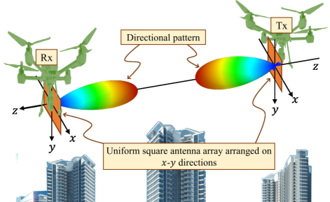
Figure 1: Illustration of an A2A link. The $z$ axis refers to the direction that extends from the Tx to the Rx node. The hovering UAVs adjust their antenna main lobes in the direction of $z$-axis.

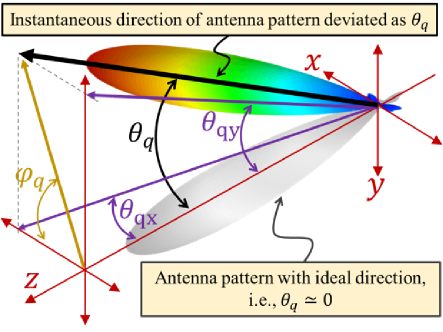
Figure 2: A graphical example of UAV orientation fluctuations. Here, the direction of antenna’s main-lobe deviates by $\theta_{q}$ from the $z$ axis. As illustrated, $\theta_{qx}$ and $\theta_{qy}$ are the instantaneous orientation fluctuations in $x-z$ and $y-z$ Cartesian coordinates, respectively.

(a)

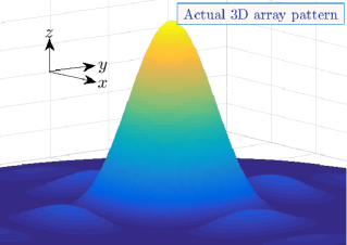
(b)

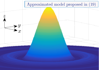
(c)

Figure 3: 3D illustration antenna pattern generated by a uniform $N_{q}\times N_{q}$ antenna array: (a) showing a $N_{q}\times N_{q}$ square array antenna arranged in $x-y$ plane; (b) 3D actual antenna pattern generated by a square array antenna arranged on the $x-y$ plane; (c) approximated antenna pattern obtained by (23).

II-A 3D Actual Antenna Pattern

Due to an approximate symmetry in the UAV vibrations in the $x$- and $y$-direction, as illustrated in Fig. 3a, we consider a uniform square array antenna, comprising $N_{q}\times N_{q}$ antenna elements with the same spacing between elements in $x$- and $y$-direction, i.e., $d_{x}=d_{y}=d_{a}$ where $d_{x}$ and $d_{y}$ are spacing between antenna elements in x- and $y$-direction, respectively. The array radiation gain is mainly formulated in the direction of $\theta_{q}$ and $\phi_{q}$. In our model, $\theta_{q}$ and $\phi_{q}$ can be defined as functions of random variables (RVs) $\theta_{qx}$ and $\theta_{qy}$ as follows:

$$\theta_{q} =\tan^{-1}\left(\sqrt{\sin^{2}(\theta_{qx})+\sin^{2}(\theta_{qy})}\right),$$

$$\phi_{q} =\tan^{-1}\left(\frac{\sin(\theta_{qy})}{\sin(\theta_{qx})}\right).$$ (1)

By taking into account the effect of all elements, the array radiation gain in direction of angles $\theta_{qx}$ and $\theta_{qy}$ will be:

$$G_{q}(\theta_{qx},\theta_{qy})=G_{a}(\theta_{qx},\theta_{qy})\,G_{e}(\theta_{qx},\theta_{qy}),$$ (2)

where $G_{a}$ is an array factor and $G_{e}$ is single element radiation pattern. From the 3GPP single element radiation pattern, $G_{e,\textrm{3dB}}=10\times\log_{10}(G_{e})$ of each single antenna element is obtained as [34]

$$G_{e\textrm{3dB}}=G_{\textrm{max}}-\min\left\{-(G_{e\textrm{3dB,1}}+G_{e\textrm{3dB,2}}),F_{m}\right\},$$ (3)

$$G_{e\textrm{3dB,1}}=-\min\left\{-12\left(\frac{\theta_{e}-90}{\theta_{e\textrm{3dB}}}\right)^{2},G_{\textrm{SL}}\right\},$$

$$G_{e\textrm{3dB,2}}=-\min\left\{-12\left(\frac{\theta_{qx}}{\phi_{e\textrm{3dB}}}\right)^{2},F_{m}\right\},$$

$$\theta_{e}=\tan^{-1}\left(\frac{\sqrt{1+\sin^{2}(\theta_{qx})}}{\sin(\theta_{qy})}\right),$$

where $\theta_{e\textrm{3dB}}=65^{\circ}$ and $\phi_{e\textrm{3dB}}=65^{\circ}$ are the vertical and horizontal 3D beamwidths, respectively, $G_{\textrm{max}}=8$ dBi is the maximum directional gain of the antenna element, $F_{m}=30$ dB is the front-back ratio, and $G_{\textrm{SL}}=30$ dB is the side-lobe level limit.

If the amplitude excitation of the entire array is uniform, then the array factor $G_{a}(\theta_{qx},\theta_{qy})$ for a square array of $N_{q}^{2}$ elements can be obtained as [35]

$$G_{a}(\theta_{qx},\theta_{qy}) =G_{0}(N_{q})\left(\frac{\sin\left(\frac{N_{q}(kd_{x}\sin(\theta_{q})\cos(\phi_{q})+\beta_{x})}{2}\right)}{N_{q}\sin\left(\frac{kd_{x}\sin(\theta_{q})\cos(\phi_{q})+\beta_{x}}{2}\right)}\right.$$

$$~{}~{}~{}~{}~{}\times\left.\frac{\sin\left(\frac{N_{q}(kd_{y}\sin(\theta_{q})\sin(\phi_{q})+\beta_{y})}{2}\right)}{N_{q}\sin\left(\frac{kd_{y}\sin(\theta_{q})\sin(\phi_{q})+\beta_{y}}{2}\right)}\right)^{2},$$ (4)

where $d_{x}=\frac{\lambda}{2}$ and $\beta_{x}$ are the spacing and progressive phase shift between the elements along the $x$ axis, respectively, and $d_{y}=\frac{\lambda}{2}$ and $\beta_{y}$ are the spacing and progressive phase shift between the elements along the $y$ axis, respectively, $k=\frac{2\pi}{\lambda}$ denotes the wave number, $\lambda=\frac{c}{f_{c}}$ denotes wavelength, $f_{c}$ denotes the carrier frequency and $c$ iss the speed of light. One of our key goals is to answer this question that for a UAV with a given instability, i.e., a given standard deviation of orientation fluctuations $\sigma_{to}$, what is the optimum values of $N_{q}$ that achieves minimum outage probability. Hence, for a fair comparison between antennas with different $N_{q}$, we consider the total radiated power of antennas with different $N_{q}$ are same. From this, we have

$$G_{0}(N_{q})=\frac{G^{\prime}_{0}}{\int_{0}^{\pi}\int_{0}^{2\pi}G(\theta_{q},\phi_{q})\sin(\theta_{q})d\theta_{q}d\phi_{q}}.$$ (5)

More details on the element and array radiation pattern is provided in [34, 35]. In addition, without loss of generality, it is assumed that $\beta_{x}=\beta_{y}=0$ and the hovering UAV sets its antenna main-lobe direction on $z$ axis. Now, the instantaneous directivity gain of a A2A link will be given by [36]

$$\mathbb{G}_{\textrm{uu}}(\theta_{{tx}},\theta_{{ty}},\theta_{{rx}},\theta_{{ry}})=G_{t}(\theta_{{tx}},\theta_{{ty}})\times G_{r}(\theta_{{rx}},\theta_{{ry}}).$$ (6)

From (6), we can see that the instantaneous directivity is a function of four independent RVs $\theta_{{tx}},\theta_{{ty}},\theta_{{rx}},\theta_{{ry}}$.

II-B Received Signal Model

Given the 3D antenna pattern described in the previous subsection, the end-to-end signal-to-interference-plus-noise ratio (SINR) of a A2A link can be obtained as

$$\gamma_{\textrm{uu}}(\alpha,\theta_{{tx}},\theta_{{ty}},\theta_{{rx}},\theta_{{ry}})\!=\!\frac{P_{t}|\alpha|^{2}h_{L}(Z)\mathbb{G}(\theta_{{tx}},\theta_{{ty}},\theta_{{rx}},\theta_{{ry}})}{\Sigma I+\sigma^{2}}\!,$$ (7)

where $\sigma^{2}$ is the thermal noise power, $\alpha$ is the small scale fading coefficient, $P_{t}$ is the transmit power, and $h_{L}(Z)$ is the path loss coefficient. Moreover, in (7), $\Sigma I=\Sigma I_{\textrm{d}}+\Sigma I_{{r}}$, where $\Sigma I_{\textrm{d}}$ and $\Sigma I_{{r}}$ are the inter-carrier interference due to Doppler spread, and radio interference due to the other Txs, respectively. Note that, by using high directional radio patterns at the Rx, $\Sigma I_{{r}}$ can be effectively eliminated [37, 38]. Furthermore, $\Sigma I_{\textrm{d}}$ is caused by Doppler spread and it is proportional to $\Sigma I_{\textrm{d}}\propto\left[1-\textrm{sinc}^{2}(f_{\textrm{d}}T_{s})\right]$, where $T_{s}$ is the symbol duration, $f_{\textrm{d}}=\frac{f_{c}\nu}{c}$ is the Doppler frequency shift, $c=3\times 10^{8}$ (in m/s) is the speed of light, $\nu$ (in m/s) is the relative moving velocity, and $f_{c}$ (in GHz) is the carrier frequency [39]. Moreover, in [40], it was shown that for a moving UAV with $\nu\leq 10$ m/s, the impact of the Doppler spread is negligible. In our setup, we assume that UAVs are hovering at a fixed position, i.e., multi-rotor UAVs or tethered balloons, and there is no relative velocity between communication nodes; therefore, there will be no Doppler spreading effect. As a result, expression in (7) can be simplified to

$$\gamma_{\textrm{uu}}(\alpha,\theta_{{tx}},\theta_{{ty}},\theta_{{rx}},\theta_{{ry}})\!=\!\frac{P_{t}|\alpha|^{2}h_{L}(Z)\mathbb{G}(\theta_{{tx}},\theta_{{ty}},\theta_{{rx}},\theta_{{ry}})}{\sigma^{2}}.$$ (8)

Since there is still no standardized results for UAV-based communications at mmW bands, we consider the results of the recent 3GPP report in [41] in order to set the path loss parameters. These parameters are valid for a BS height up to 150 m and are expressed as follows:

$$h_{\textrm{L,dB}}(Z) =-20\log_{10}\left(\frac{40\pi Zf_{c}}{3}\right)$$ (9)

$$+\min\left\{0.03h_{b}^{1.73},10\right\}\times\log_{10}(Z)$$

$$+\min\left\{0.044h_{b}^{1.73},14.77\right\}-0.002\,Z\log_{10}(h_{b}),$$

where $h_{b}$ (in meter) is the average of building height of city. Moreover, from the measurement results provided in [42], for a low altitude communication link between UAVs, Rician and Nakagami distributions were shown to be highly promising models that can be mathematically fitted into the experimentally measured data. Since the Nakagami distribution is a universal model that can capture various channel conditions, we apply it to model small-scale fading. Let $\alpha$ be a Nakagami random variable (RV). Hence, $\zeta=\alpha^{2}$ will be a normalized Gamma RV given by:

$$f_{\zeta}(\zeta)=\frac{m^{m}\zeta^{m-1}}{\Gamma(m)}\exp(-m\zeta),~{}~{}~{}\zeta>0,$$ (10)

where $m$ is the Nakagami fading parameter and $\Gamma(\cdot)$ is the Gamma function [42].

In practice, a highly directional beam is used to compensate the high free-space path loss at the mmW band. Hence, in addition to the channel fading, fluctuations in the orientation of the UAVs (due to the effect of wind, mechanical and control system flaws, antenna and BS payload, etc.) can lead to beam misalignment and adversely affect the link performance and channel capacity. To capture these effects, we define the outage capacity, i.e., the probability with which the instantaneous capacity falls bellow a certain threshold $\mathcal{C}_{\textrm{th}}$, as the figure of merit to determine the reliability of the considered UAV-based communication system. The outage capacity can be defined as follows:

$$\mathbb{P}_{\textrm{out}} ={\textrm{Pr}}\{\log_{2}(1+\gamma)<\mathcal{C}_{\textrm{th}}\}=F_{\gamma}(\gamma_{\textrm{th}}),$$ (11)

where $F_{x}(\cdot)$ is the cumulative distribution function (CDF) of RV $x$, $\gamma$ is the end-to-end signal-to-noise ratio (SNR), and $\gamma_{\textrm{th}}=2^{\mathcal{C}_{\textrm{th}}}-1$ is the SNR threshold.

From (8), it can be observed that the end-to-end SNR is composed of the deterministic loss parameter $h_{L}$, and several RVs, i.e., the small-scale fading coefficient $\alpha$, the AoD deviations due to $\theta_{{tx}}$ and $\theta_{{ty}}$, and the AoA deviations $\theta_{{rx}}$ and $\theta_{{ry}}$. To assess the benefits of deploying UAV-based mmW communications under the aforementioned RVs, one important challenge is to accurately model the channel, which can then be used for easily evaluating the performance of hovering UAV-based mmW links without performing time-consuming simulations. Accordingly, in the next section, we derive the closed-form expressions of the SNR distribution at the Rx by taking into account the unique characteristics of mmW links along with the effects of UAV random vibrations and orientation fluctuations.

III Analytical Channel Models

Next, we first develop a channel model for the A2A link. Then, for simpler A2G and G2A cases, we obtain more tractable channel models.

III-A UAV-to-UAV Link

Theorem 1. The probability density function (PDF) of end-to-end SNR of A2A link can be well modeled as

$$f_{\gamma_{\textrm{uu}}}(\gamma_{\textrm{uu}})=\!\sum_{d_{r}=0}^{jD-1}\sum_{d_{t}=0}^{jD-1}\!\mathbb{R}_{d_{t},d_{r}}\gamma_{\textrm{uu}}^{m-1}\exp\!\left(\!-\frac{m\sigma^{2}}{P_{t}h_{L}(Z)\mathbb{R}^{\prime}_{d_{t},d_{r}}}\,\gamma_{\textrm{uu}}\!\right)\!,$$ (12)

where for $d_{t}\,\&\,d_{r}\in\{0,1,...,jD-1\}$ and $j\in\{1,2\}$, we have

$$\mathbb{R}_{d_{t},d_{r}}=\frac{\mathbb{J}_{d_{t},d_{r}}(\theta^{\prime}_{t,xy},\theta^{\prime}_{r,xy},\sigma^{2}_{to},\sigma^{2}_{ro})}{\Gamma(m)}\left(\frac{m\,\sigma^{2}}{P_{t}h_{L}(Z)\mathbb{R}^{\prime}_{d_{t},d_{r}}}\right)^{m},$$

$$\left\{\begin{array}[]{ll}\mathbb{R}^{\prime}_{0,0}&\!\!\!\!\!\!=4k^{4}d_{a}^{4}G_{0}^{\prime\prime}(N_{t})G_{0}^{\prime\prime}(N_{r}),\\ \mathbb{R}^{\prime}_{d_{t},0}&\!\!\!\!\!\!=2k^{2}d_{a}^{2}G_{0}^{\prime\prime}(N_{t})G_{0}^{\prime\prime}(N_{r})\frac{D^{2}\left(1-\cos\left(\frac{d_{t}kd_{a}}{D}\right)\right)}{d_{t}^{2}},\\ \mathbb{R}^{\prime}_{0,d_{r}}&\!\!\!\!\!\!=2k^{2}d_{a}^{2}G_{0}^{\prime\prime}(N_{t})G_{0}^{\prime\prime}(N_{r})\frac{D^{2}\left(1-\cos\left(\frac{d_{r}kd_{a}}{D}\right)\right)}{d_{r}^{2}},\\ \mathbb{R}^{\prime}_{d_{t},d_{r}}&\!\!\!\!\!\!=4G_{0}^{\prime\prime}(N_{t})G_{0}^{\prime\prime}(N_{r})\frac{D^{4}\left(\sin^{2}\left(\frac{d_{t}kd_{a}}{2D}\right)\sin^{2}\left(\frac{d_{r}kd_{a}}{2D}\right)\right)}{d_{t}^{2}\,d_{r}^{2}},\end{array}\right.$$

$$\mathbb{J}_{d_{t},d_{r}}(\theta^{\prime}_{t,xy},\theta^{\prime}_{r,xy},\sigma^{2}_{to},\sigma^{2}_{ro})=J_{d_{t}}(\theta^{\prime}_{t,xy},\sigma^{2}_{to})J_{d_{r}}(\theta^{\prime}_{r,xy},\sigma^{2}_{ro}),$$

$$J_{d_{q}}(\theta^{\prime}_{q,xy},\sigma^{2}_{qo})=M\!\left(\frac{\theta^{\prime}_{q,xy}}{\sigma_{qo}},\frac{d_{q}}{DN_{q}\sigma_{qo}}\right)\!-\!M\left(\!\frac{\theta^{\prime}_{q,xy}}{\sigma_{qo}},\frac{d_{q}+1}{DN_{q}\sigma_{qo}}\!\right)\!.$$

In addition, $G_{0}^{\prime\prime}(N_{q})=0.2025\times 10^{\frac{G_{\textrm{max}}}{10}}G_{0}(N_{q})$ and $M(a,b)$ is the Marcum Q-function.

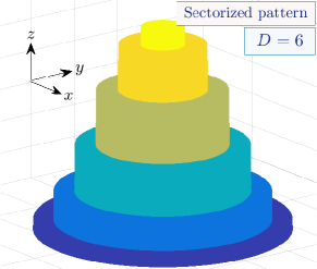
(a)

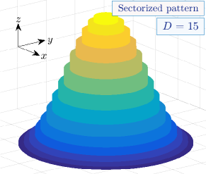
(b)

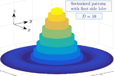
(c)

Figure 4: Sectorized antenna pattern obtained from (A) for (a) $D=6$ and $j=1$, (b) $D=15$ and $j=1$, and (c) $D=10$ and $j=2$.

Proof:

Please refer to Appendix A. ∎

As one can observe from (12), the effects of large- and small-scale fading characterized by $\alpha$, $m$ and $h_{L}(Z)$, UAVs stability characterized by $\theta^{\prime}_{tx}$, $\theta^{\prime}_{ty}$, $\theta^{\prime}_{rx}$, $\theta^{\prime}_{ry}$, $\sigma^{2}_{to}$ and $\sigma^{2}_{ro}$, and antenna pattern specifications characterized by $N_{t}$ and $N_{r}$, are incorporated into the closed-form channel PDF. For instance, in the proposed analytical results, antenna directivity gain and beamwidth are tuned by $N_{q}$ that by increasing $N_{q}$ antenna directivity gain increases with the decreasing beamwidth. In addition, the strength of UAV instability is modeled by $\sigma_{{to}}$, $\sigma_{{ro}}$, $\theta^{\prime}_{{tx}}$, $\theta^{\prime}_{{ty}}$, $\theta^{\prime}_{{rx}}$ and $\theta^{\prime}_{{ry}}$, and the small-scale fading strength is characterized by $m$.

We note that the accuracy of the derived analytical expressions in Theorem 1 depends on the variable $D$ that is used for the approximation of antenna pattern. The optimal value of $D$ is its minimum value that satisfies a predefined accuracy. As seen later, $D=30$ is a good choice and achieves the analytical results close to the simulation results.

Moreover, note that parameter $j\in\{1,2\}$ is another parameter that controls the accuracy of the derived channel PDF. The accuracy of the derived channel model for both values of $j$ are investigated in the Section III using simulation results.

Now we derive the analytical expression for CDF of end-to-end SNR of A2A link which is useful for outage probability analysis.

Lemma 1. The CDF of end-to-end SNR of A2A link is obtained as

$$F_{\gamma_{\textrm{uu}}}(\gamma_{\textrm{uu}}) =\sum_{d_{r}=0}^{jD-1}\sum_{d_{t}=0}^{jD-1}\!\mathbb{R}_{d_{t},d_{r}}\left(\frac{P_{t}h_{L}(Z)\mathbb{R}^{\prime}_{d_{t},d_{r}}}{m\sigma^{2}}\right)^{m}$$

$$~{}~{}~{}~{}~{}~{}~{}~{}~{}~{}~{}~{}~{}~{}\times\mathcal{V}\left(m,\frac{m\sigma^{2}}{P_{t}h_{L}(Z)\mathbb{R}^{\prime}_{d_{t},d_{r}}}\,\gamma_{\textrm{uu}}\right),$$ (13)

where $\mathcal{V}(.,.)$ is the incomplete Gamma function.

Proof:

Using (12) and [43, (8.350.1)], the CDF of RV $\gamma_{\textrm{uu}}$ is derived in (III-A). ∎

III-B Ground-to-UAV and UAV-to-Ground Links

Next we derive the channel distribution of G2A and A2G links.

Lemma 2. The PDF and CDF of end-to-end SNR of G2A link are obtained respectively as

$$f_{\gamma_{\textrm{gu}}}(\gamma_{\textrm{gu}}) =\sum_{d_{r}=0}^{jD-1}\frac{J_{d_{r}}(\theta^{\prime}_{r,xy},\sigma^{2}_{ro})(J^{\prime}_{d_{r}})^{m}}{\Gamma(m)(P_{t}h_{L}(Z))^{m}}$$

$$~{}~{}~{}~{}~{}~{}~{}~{}~{}~{}~{}~{}\times\gamma_{\textrm{gu}}^{m-1}\exp\left(-\frac{J^{\prime}_{d_{r}}\gamma_{\textrm{gu}}}{P_{t}h_{L}(Z)}\right),$$ (14)

and

$$F_{\gamma_{\textrm{gu}}}(\gamma_{\textrm{gu}}) =\sum_{d_{r}=0}^{jD-1}\frac{J_{d_{r}}(\theta^{\prime}_{r,xy},\sigma^{2}_{ro})}{\Gamma(m)}\times\mathcal{V}\left(m,\frac{J^{\prime}_{d_{r}}\,\gamma_{\textrm{gu}}}{P_{t}h_{L}(Z)}\right),$$ (15)

where

$$J^{\prime}_{d_{r}}\!=\!\left\{\!\!\!\begin{array}[]{ll}\frac{m\,\sigma^{2}}{2k^{2}d_{a}^{2}G_{\textrm{t,max}}G_{0}^{\prime\prime}(N_{r})},{}{}{}&d_{r}=0,\\ \\ \frac{m\,\sigma^{2}}{G_{t,\textrm{max}}G_{0}^{\prime\prime}(N_{r})\frac{D^{2}\left(1-\cos\left(\frac{d_{r}kd_{a}}{D}\right)\right)}{d_{r}^{2}}},\!\!&d_{r}\in\{0,...,N_{r}\}.\end{array}\right.$$ (19)

Proof:

In practice, the orientation fluctuations of a fixed ground node is much smaller than the UAV node. Hence, for a ground node, we assume $\theta_{q}\simeq 0$. Under such conditions, it is assumed that the fixed ground antenna is perfectly aligned to the antenna mounted on UAV. Hence, the ground antenna gain can be well approximated by its maximum gain at the main-lobe. From this, for G2A link, (6) can be simplified as

$$\mathbb{G}_{\textrm{gu}}(\theta_{{rx}},\theta_{{ry}})=G_{{t,max}}\times G_{r}(\theta_{{rx}},\theta_{{ry}}),$$ (20)

where $G_{t,\textrm{max}}=G_{t}(\theta_{{tx}}\simeq 0,\theta_{{ty}}\simeq 0)$. From (20) and similar to the derivation of (A), we have

$$f_{\mathbb{G}_{\textrm{gu}}}(\mathbb{G}_{\textrm{gu}})=J_{0}(\theta^{\prime}_{r,xy},\sigma^{2}_{ro})\,\delta\left(G_{r}-2k^{2}d_{a}^{2}G_{t,\textrm{max}}G_{0}^{\prime\prime}(N_{r})\right)$$ (21)

$$~{}~{}~{}~{}~{}~{}~{}~{}~{}+\sum_{d_{r}=1}^{jD-1}J_{d_{r}}(\theta^{\prime}_{r,xy},\sigma^{2}_{ro})$$

$$~{}~{}~{}~{}~{}~{}~{}~{}~{}\times\delta\left(G_{r}-G_{t,\textrm{max}}G_{0}^{\prime\prime}(N_{r})\frac{D^{2}\left(1-\cos\left(\frac{d_{r}kd_{a}}{D}\right)\right)}{d_{r}^{2}}\right).$$

Finally, using (8), (10) and (21), the closed-form expression of the G2A channel PDF is derived in (III-B). ∎

p s

As one can observe, the proposed channel model in (III-B) is a simple function of end-to-end SNR $\gamma_{\textrm{gu}}$. However, despite the simplicity and tractability, the proposed closed-form channel model composes the effects of large- and small-scale fading characterized by $\alpha$, $m$ and $h_{L}(Z)$, UAVs stability characterized by $\theta^{\prime}_{rx}$, $\theta^{\prime}_{ry}$, and $\sigma^{2}_{ro}$, and antenna pattern specifications characterized by $N_{t}$ and $N_{r}$.

The channel distribution of the A2G link can be obtained similarly from (III-B) by swapping subscript $t$ with subscript $r$ and vice versa.

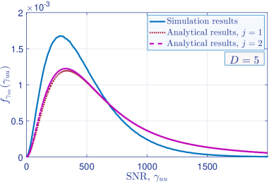
(a)

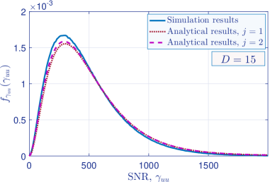
(b)

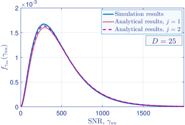
(c)

Figure 5: Channel distribution of A2A link when $\sigma^{2}_{to}=\sigma^{2}_{ro}=1^{o}$, $\theta^{\prime}_{tx}=\theta^{\prime}_{ty}=0.5^{o}$ and $\theta^{\prime}_{rx}=\theta^{\prime}_{ry}=1^{0}$, for a) $D=5$, b) $D=15$, and c) $D=25$.

IV Simulation Results

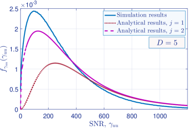
(a)

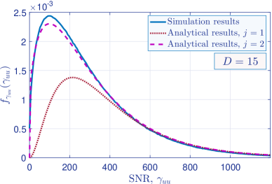
(b)

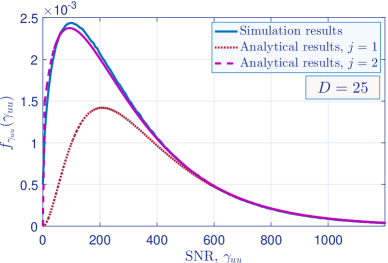
(c)

Figure 6: Channel distribution of A2A link when $\sigma^{2}_{to}=\sigma^{2}_{ro}=3^{o}$, $\theta^{\prime}_{tx}=\theta^{\prime}_{ty}=1^{o}$ and $\theta^{\prime}_{rx}=\theta^{\prime}_{ry}=0.5^{o}$, for a) $D=5$, b) $D=15$, and c) $D=25$.

For our simulations, we consider standard values for system parameters, as follows. The carrier frequency $f_{c}=50$ GHz, average building height $h_{b}=30$ m, thermal noise power $\sigma^{2}=-110$ dBm, Nakagami fading parameter $m=3$, transmit power $P_{t}=20$ dBm, and SNR threshold $\gamma_{\textrm{th}}=10$ dB.

IV-1 Accuracy of the Derived Channel Models

The accuracy of the proposed channel PDF for a A2A link is evaluated in Figs. 5 and 6 for two different values of the UAV’s instability parameters $\sigma_{to}=\sigma_{ro}=1^{o}$ and $\sigma_{to}=\sigma_{ro}=3^{o}$, respectively. The accuracy of the analytical channel model is validated using Monte Carlo simulations. For Monte Carlo simulations, we generate $5\times 10^{7}$ independent RVs $\alpha$, $\theta_{{tx}}$, $\theta_{{ty}}$, $\theta_{{rx}}$, and $\theta_{{ry}}$. For each $5\times 10^{7}$ independent run, we calculate antenna pattern from actual model given in (2)-(6), and then, calculate $5\times 10^{7}$ instantaneous SNR from (8). From (12), $D$ and $j\in\{1,2\}$ are two parameters that impact on the validity of channel PDF. The variable $D$ is used for approximating the antenna pattern. The optimal value of $D$ is its minimum value that satisfies a predefined accuracy. Parameter $j\in\{1,2\}$ is another parameter that determines the accuracy of the derived channel PDF. The results of Figs. 5 and 6 are plotted for different values of $D$ and two different values of $j=1$ and $j=2$. Figs. 5 and 6 demonstrate that $D=25$ can be a good choice. Moreover, by comparing the results of these figure, it can be observed that for UAVs with higher angular stability (lower $\sigma_{to}$ and $\sigma_{ro}$), $j=1$ is a good choice. Meanwhile, by decreasing stability (increasing $\sigma_{to}$ and $\sigma_{ro}$), the accuracy of analytical channel model decreases for $j=1$. Under this condition, the channel must be modeled with main-lobe along with the first side-lobe, i.e., $j=2$.

IV-2 Performance Analysis and Optimal Pattern Selection

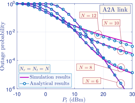
Figure 7: Outage probability of A2A link for $\sigma_{to}=\sigma_{ro}=2^{o}$, $\theta^{\prime}_{tx}=\theta^{\prime}_{ty}=\theta^{\prime}_{rx}=\theta^{\prime}_{ry}=0.5^{o}$, and different values of $N_{t}$ and $N_{r}$.

Next, the performance of the considered UAV-based mmW link is studied in terms of outage probability. To study the impact of antenna pattern on the system performance, in Fig 7, the outage probability of A2A link is plotted versus $P_{t}$ and for different values of $N_{t}=N_{r}=N$. As we observe, the accuracy of the derived closed-form expression for the outage probability is verified via our simulation results. From this figure, we can see that lower values for $N$ achieve a better performance at a high $P_{t}$ regime. However, at a low $P_{t}$ regime, higher values of $N$ achieve better performance. This can be justified since the poor SNR at low values of $P_{t}$ can be compensated by high directional antenna pattern. Meanwhile, at high values of $P_{t}$, the outage probability of high directional beam is floored due to the UAVs’ orientation fluctuations. Under such conditions, antenna pattern must be selected wider to compensate UAVs’ orientation fluctuations.

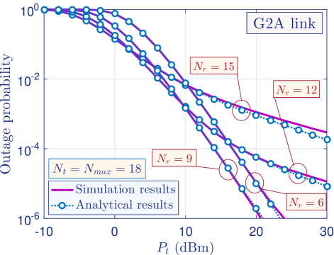
Figure 8: Outage probability of G2A link for $\sigma_{ro}=2^{o}$, $\theta^{\prime}_{rx}=\theta^{\prime}_{ry}=0.5^{o}$, $N_{t}=N_{\textrm{max}}=18$, and different values of $N_{r}$.

In Fig. 8, we investigate the impact of antenna pattern on the outage probability of G2A link. As mentioned, for a G2A link, due to the high stability of a fixed ground antenna compared to the aerial antenna, we consider $N_{t}=N_{\textrm{max}}=18$. The results of Fig. 8 are obtained for $\sigma_{ro}=2^{o}$, $\theta^{\prime}_{rx}=\theta^{\prime}_{ry}=0.5^{o}$ and $Z=2000$ m. Similar to the A2A link, we can see that higher values of $N_{r}$ achieve a better performance at a low $P_{t}$ regime, and vice versa. Meanwhile, we observe a perfect match between the analytical and simulation-based results which validates the accuracy of our derived analytical expressions for G2A link. By comparing the results of Figs. 7 and 8, as expected, we can observe that the G2A link achieves better performance compared to the A2A link.

To have a better comparing between A2A and G2A links, we evaluated the outage probability of both links in Fig. 9 as a function of the link length, $Z$. The results of Fig. 9 are provided for $P_{t}=14$ dBm and two different values for the UAV instability factor $\sigma_{ro}=2^{o}$ and $\sigma_{ro}=4^{o}$. As expected, by increasing link length, the channel loss increases, and thus, performance degrades. However, increasing link length has a more sever effect on the A2A link compared to the G2A link. Fig. 9 shows that, for a link length greater than 2000 m, a G2A link with $\sigma_{ro}=4^{o}$ achieves a lower outage probability than an A2A link with $\sigma_{ro}=2^{o}$. The results of Fig. 9 are provided for the constant values for $N_{t}$ and $N_{r}$. However, we expect that by varying link length, the optimal value for $N_{t}$ and $N_{r}$ change.

In Fig. 10, we investigate the outage probability of A2A link versus $Z$ and $N$ in order to shed light on the impact of the link length on the optimal value of $N$. This figure clearly shows that by varying link length, the optimal value for $N$ changes. As the link length increases, the optimal value for $N$ must be increased to compensate for the additional channel loss due to the larger link length. For instance, from the results of Fig. 10, we observe that, by increasing the link length from 1000 to 3000 m, the optimal value for $N$ increases from 9 to 15.

The strength of UAV’s orientation fluctuations is the another important parameter that can affect on the optimal value for antenna pattern, $N$. In Fig. 11, the outage probability of A2A link is plotted versus $N_{t}$ and $\sigma_{to}$ for a special symmetrical case wherein $\sigma_{to}=\sigma_{ro}$ and $N_{t}=N_{r}=N$. From Fig. 11, we can see that, for the symmetrical case, the optimal value for $N_{t}$ decreases by increasing $\sigma_{to}$. For instance, by increasing $\sigma_{to}=1^{o}$ to $\sigma_{to}=3^{o}$, the optimal value for $N_{t}$ decreases from 16 to 9. This can be justified since by increasing $\sigma_{to}$, the beamwidth of antenna pattern must be increases to compensate the orientation fluctuations of the hovering UAV. Hence, the antenna gain must be decreased in order to increase antenna beamwidth. The results of Fig. 11 are provided for a symmetrical case.

To get a better insight about a more general case, in Figs. 12a and 12b we investigate the outage probability of an A2A link versus $N_{t}$ and $N_{r}$ for two different UAVs’ angular stability where $\sigma_{to}\neq\sigma_{ro}$. From these figures, we observe that by changing $N_{t}$ and $N_{r}$, the outage probability changes, significantly. More importantly, by changing the angular stability, the optimal antenna pattern changes. For instance, by changing UAVs’ angular stability from $\sigma_{to}=3^{o},\sigma_{ro}=2^{o}$ to $\sigma_{to}=4^{o},\sigma_{ro}=1.5^{o}$, the optimal values for $N_{t}$, $N_{r}$ changes from $N_{t}=7,N_{r}=10$ to $N_{t}=5,N_{r}=13$. Here, we note that, in addition to the mechanical control system of UAV, air pressure and wind speed can affect on the UAV’s angular stability. Since air pressure and wind speed continuously changes in the day time, it is reasonable to expect that the UAV’s angular stability changes in day time. Hence, to achieve a reliable communication link for the considered UAV-based system, we propose that to design the square array antenna with maximum number of antenna elements, $N_{\textrm{max}}\times N_{\textrm{max}}$. Then, for any given angular stability, which continuously changes in the order of several minutes to several hours, we only activate $N_{t}\times N_{t}$ Tx antenna elements and $N_{r}\times N_{r}$ Rx antenna elements of $N_{\textrm{max}}\times N_{\textrm{max}}$ that achieves a minimum outage probability where $N_{t},N_{r}\in\{1,...,N_{\textrm{max}}\}$. Formally, the problem can be formulated as

$$\mathop{{\textrm{ min}}}\limits_{N_{rs},N_{rd},\psi_{s},\psi_{d}}~{}~{}\mathbb{P}_{\textrm{out}},$$ (22)

$$~{}~{}~{}~{}~{}~{}\textrm{ s.t.}~{}~{}~{}~{}~{}~{}~{}~{}N_{rs},N_{rd}\in\{1,N_{\textrm{max}}\}.$$

For different values of $\sigma_{to}$ and $\sigma_{ro}$, the optimal number of $N_{t}$, $N_{r}$, and the corresponding minimum achievable outage probabilities are provided in Table I. The optimal results are obtained by simulations. The simulation results are obtained by performing Monte Carlo simulations with $5\times 10^{7}$ independent runs and using a computer with an Intel i7-3632QM CPU running at 2.20 GHz with 8 GB RAM. Under such conditions, the running time of the optimization problem takes approximately $500$ s.

Finally, to confirm the accuracy of our derived analytical expressions, as a suboptimal method, we numerically find $N_{t}$ and $N_{r}$ by using (III-A). The simulation results of Table I confirm the validity of the numerical results that only requires running time $\simeq 1$. Note that, for $5\times 10^{7}$ independent runs, the simulation results is valid when $\mathbb{P}_{\textrm{out}}>10^{6}$. For high quality of services with lower outage probability, we require to more independent runs that increases running time. Moreover, in (22), we only optimize two parameters $N_{t}$ and $N_{r}$. However, one can use analytical expressions provided in this paper to optimize the other parameters such as code rate, modulation size, UAV’s aerial position and so on, in an extremely time efficient manner.

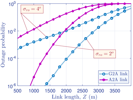
Figure 9: Comparison of the outage probability of A2A and G2A links versus link length for two different conditions, $\sigma_{ro}=2^{o}$ and $\sigma_{ro}=4^{o}$. For G2A link, $N_{t}=N_{\textrm{max}}$ and $N_{r}=8$, and for A2A link, $\sigma_{to}=\sigma_{ro}$ and $N_{t}=N_{r}=8$.

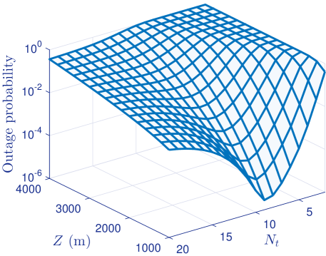
Figure 10: Outage probability of A2A link versus link length and $N_{t}$ for $N_{r}=N_{t}$, $\sigma_{to}=\sigma_{ro}=2$ mrad, and $P_{t}=15$ dBm.

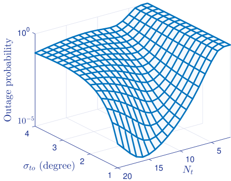
Figure 11: Outage probability of A2A link versus $\sigma_{to}$ and $N_{t}$ when $\sigma_{ro}=\sigma_{to}$ and $N_{r}=N_{t}=N$.

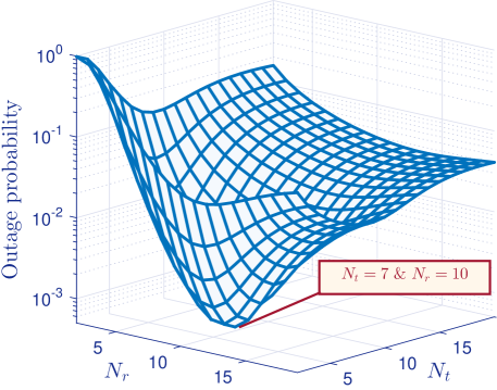
(a)

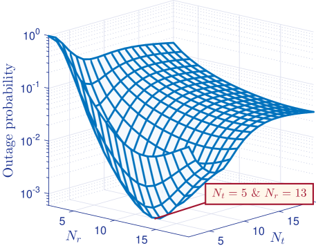
(b)

Figure 12: Outage probability of A2A link versus $N_{t}$ and $N_{r}$ for two different scenario with different instabilities: (a) for $\sigma_{to}=3^{o}$ and $\sigma_{ro}=2^{o}$, and (b) for $\sigma_{to}=4^{o}$ and $\sigma_{ro}=1.5^{o}$.

V Conclusion

In this paper, we have studied the performance of UAV-based mmW links when UAVs are equipped with square array antenna. Accordingly, we have characterized the UAV-based mmW channels by considering the large scale path loss, small scale fading along with antenna patterns as well as the random effect of UAVs’ angular vibrations. For performance analysis, we have derived closed-form statistical channel models for A2A, G2A, and A2G channels. We have then verified the accuracy of analytical models by employing Monte Carlo simulations. Our analytical results have made it possible to find the optimal antenna directivity gain for designing a reliable UAV-based mmW communications under different levels of stability of UAVs without resorting to time-consuming simulations.

Table I: Comparison of the Optimal values for $N_{\rm t}$ and $N_{\rm r}$ obtained by simulation and numerical results to achieve minimum outage probability over A2A link for different conditions of UAV instabilities.

Angular instability		Suboptimal values obtained by analytical results				Optimal values obtained by simulation results
$~{}~{}~{}\sigma_{to}~{}~{}~{}$	$\sigma_{ro}$	$~{}~{}N_{t}~{}~{}$	$~{}~{}N_{r}~{}~{}$	$\mathbb{P}_{\textrm{out}}$	Running time	$~{}~{}N_{t}~{}~{}$	$~{}~{}N_{r}~{}~{}$	$\mathbb{P}_{\textrm{out}}$	Running time
$5^{o}$	$3^{o}$	4	7	$1.52\times 10^{-3}$	$\simeq 1$ s	4	8	$1.35\times 10^{-3}$	$\simeq 500$ s
$2^{o}$	$4^{o}$	9	5	$1.03\times 10^{-4}$	$\simeq 1$ s	9	5	$1.06\times 10^{-4}$	$\simeq 500$ s
$3^{o}$	$2^{o}$	6	9	$2.85\times 10^{-5}$	$\simeq 1$ s	6	9	$2.76\times 10^{-5}$	$\simeq 500$ s
$1^{o}$	$2^{o}$	15	8	$2.39\times 10^{-7}$	$\simeq 1$ s	$\mathbb{P}_{\textrm{out}}<10^{-6}$ and requires more independent runs

Appendix A Proof of Theorem 1

Note that $\gamma_{\textrm{uu}}$ is a function of five RVs $\alpha$, $\theta_{{tx}}$, $\theta_{{ty}}$, $\theta_{{rx}}$ and $\theta_{{ry}}$. To derive a tractable analytical model for $\gamma_{\textrm{uu}}$, we must first calculate the analytical model for $\mathbb{G}_{\textrm{uu}}(\theta_{{tx}},\theta_{{ty}},\theta_{{rx}},\theta_{{ry}})$ which is a functions of $G_{t}(\theta_{{tx}},\theta_{{ty}})$ and $G_{r}(\theta_{{rx}},\theta_{{ry}})$. As we observe from (2), (3) and (II-A), the array antenna gain $G_{{q}}$ is a complex function of $\theta_{qx}$ and $\theta_{qy}$, where subscript ${q}\in\{{t},{r}\}$ denotes, respectively, the Tx and Rx antenna. After an exhaustive search over the actual pattern model provided in (2), we obtain a simpler mathematical function for $G_{\textrm{q}}$ as

$$G_{q}(\theta_{{qx}},\theta_{qy})\simeq G_{0}^{\prime\prime}(N_{q})\,\frac{1-\cos(N_{q}kd_{a}\sqrt{\theta_{qx}^{2}+\theta_{qy}^{2}})}{N_{q}^{2}\left(\theta_{qx}^{2}+\theta_{qy}^{2}\right)},$$ (23)

where $G_{0}^{\prime\prime}(N_{q})=0.2025\times 10^{\frac{G_{\textrm{max}}}{10}}G_{0}(N_{q})$. For comparison with the actual antenna pattern obtained by (2), the 3D graphical pattern generated by (23) is plotted in Fig. 3c. For a better comparison, we also plot the 2D pattern generated by (23) in Fig. 13 versus $\theta_{qx}$ for different values of $\theta_{qy}$. As we observe, an exact match exists between approximated model and actual antenna pattern, specially, at the main-lobe.

Let us denote $\theta_{{q,xy}}=\sqrt{\theta_{qx}^{2}+\theta_{qy}^{2}}$. As mentioned, the RVs $\theta_{qx}$ and $\theta_{qy}$ are modeled as $\theta_{qx}\sim\mathcal{N}(\theta^{\prime}_{qx},\sigma^{2}_{qo})$, and $\theta_{qy}\sim\mathcal{N}(\theta^{\prime}_{qy},\sigma^{2}_{qo})$. Hence, the PDF of $\theta_{{q,xy}}$ becomes Rician

$$f_{\theta_{{q,xy}}}(\theta_{{q,xy}})\!=\!\frac{\theta_{{q,xy}}}{\sigma_{qo}^{2}}\exp\!\left(\!-\frac{\theta_{{q,xy}}^{2}+\theta_{{q,xy}}^{\prime 2}}{2\sigma_{qo}^{2}}\!\right)I_{0}\!\left(\!\frac{\theta_{{q,xy}}\theta_{{q,xy}}^{\prime}}{\sigma_{qo}^{2}}\!\right),$$ (24)

where $\theta_{{q,xy}}^{\prime}=\sqrt{\theta_{qx}^{\prime 2}+\theta_{qy}^{\prime 2}}$, and $I_{0}(.)$ is the modified Bessel function of the first kind with order zero. Moreover, Fig. 2 clearly shows that the main power is radiated at main-lobe. Therefore, for a point-to-point link, it is reasonable to approximate the actual antenna array gain by only its main-lobe and for much more precision, main-lobe along with the first side-lobe. Now, by sectorizing (23), we propose a simpler sectorized model given by

$$G_{q}(\theta_{qx},\theta_{qy}) \simeq G_{q}(\theta_{{q,xy}},D)=2k^{2}d_{a}^{2}G_{0}^{\prime\prime}(N_{q})\,\Pi\left(DN_{q}\theta_{{q,xy}}\right)$$

$$+ G_{0}^{\prime\prime}(N_{q})\sum_{i=1}^{j\,D-1}\frac{D^{2}\left(1-\cos\left(\frac{ikd_{a}}{D}\right)\right)}{i^{2}}$$

$$\times \left[\Pi\left(\frac{DN_{q}|\theta_{{q,xy}}|}{i+1}\right)-\Pi\left(\frac{DN_{q}|\theta_{{q,xy}}|}{i}\right)\right],$$ (25)

where $\Pi(x)=\left\{\begin{array}[]{rl}1&~{}~{}~{}{\rm for}~{}~{}~{}|x|\leq 1\\ 0&~{}~{}~{}{\rm for}~{}~{}~{}|x|>1\\ \end{array}\right.$ and $j\in\{1,2\}$ whereby $j=1$ is used when the main-lobe of pattern is considered and for more precision, $j=2$ is used when main-lobe along with the first side-lobe is considered. For $j=1$, Figs. 4a and 4b show the sectorized model for $D=6$ and $D=15$, respectively. Obviously, the accuracy of the proposed model increases by increasing $D$ at the cost of more complexity. Hence, choosing an optimal value for $D$ involves a tradeoff between tolerable complexity and desirable accuracy. Moreover, in Fig. 4c, we show an example of sectorized model for $j=2$ and $D=10$.

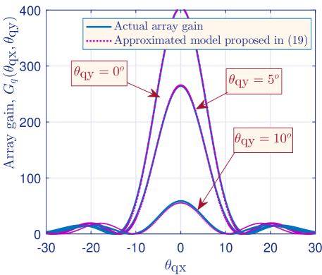
Figure 13: Approximated antenna pattern proposed in (23) and comparing its validity with actual antenna pattern characterized in Section II for $N_{q}=8$.

From (24), (A) and using [44], after some mathematical manipulations, the PDF of $G_{q}(\theta_{qx},\theta_{qy})$ can be approximated as

$$f_{G_{q}}(G_{q})=J_{0}(\theta^{\prime}_{q,xy},\sigma^{2}_{qo})\,\delta\left(G_{q}-2k^{2}d_{a}^{2}G_{0}^{\prime\prime}(N_{q})\right)$$ (26)

$$~{}~{}~{}~{}~{}~{}~{}~{}~{}~{}~{}~{}~{}+\sum_{d_{q}=1}^{jD-1}J_{d_{q}}(\theta^{\prime}_{q,xy},\sigma^{2}_{qo})$$

$$~{}~{}~{}~{}~{}~{}~{}~{}~{}~{}~{}~{}~{}\times\delta\left(G_{q}-G_{0}^{\prime\prime}(N_{q})\frac{D^{2}\left(1-\cos\left(\frac{d_{q}kd_{a}}{D}\right)\right)}{d_{q}^{2}}\right),$$

where for $d_{q}\in\{0,1,...,jD-1\}$, we have

$$J_{d_{q}}(\theta^{\prime}_{q,xy},\sigma^{2}_{qo})=M\!\left(\frac{\theta^{\prime}_{q,xy}}{\sigma_{qo}},\frac{d_{q}}{DN_{q}\sigma_{qo}}\right)\!-\!M\left(\!\frac{\theta^{\prime}_{q,xy}}{\sigma_{qo}},\frac{d_{q}+1}{DN_{q}\sigma_{qo}}\!\right)\!,$$ (27)

and $M(a,b)$ is the Marcum Q-function and can be formulated as

$$M(a,b)=\int_{b}^{\infty}x\exp\left(-\frac{x^{2}+a^{2}}{2}\right)I_{0}(ax).$$ (28)

Note that the Marcum Q-function is an standard function which can be readily computed. From (6) and (26), the PDF of RV $\mathbb{G}_{\textrm{uu}}(\theta_{{tx}},\theta_{{ty}},\theta_{{rx}},\theta_{{ry}})$ conditioned on RV $G_{r}(\theta_{{tx}},\theta_{{ty}})$ is derived as

$$f_{\mathbb{G}_{\textrm{uu}}|G_{r}}(\mathbb{G}_{\textrm{uu}})=\frac{J_{0}(\theta^{\prime}_{t,xy},\sigma^{2}_{to})}{G_{r}}\,\delta\left(\frac{\mathbb{G}_{\textrm{uu}}}{G_{r}}-2k^{2}d_{a}^{2}G_{0}^{\prime\prime}(N_{t})\right)+$$

$$\sum_{d_{t}=1}^{jD-1}\!\frac{J_{d_{t}}(\theta^{\prime}_{t,xy},\sigma^{2}_{to})}{G_{r}}\delta\!\left(\!\frac{\mathbb{G}_{\textrm{uu}}}{G_{r}}-G_{0}^{\prime\prime}(N_{t})\frac{D^{2}\!\left(\!1\!-\!\cos\left(\frac{d_{t}kd_{a}}{D}\right)\!\right)}{d_{t}^{2}}\!\right).$$ (29)

Using (26) and (A) and after some derivations, the PDF of $\mathbb{G}_{\textrm{uu}}$ as a function of $N_{t}$, $N_{r}$, $\theta^{\prime}_{t,xy}$, $\theta^{\prime}_{r,xy}$, $\sigma^{2}_{to}$ and $\sigma^{2}_{to}$, is derived in (A).

$$f_{\mathbb{G}_{\textrm{uu}}}(\mathbb{G}_{\textrm{uu}})=\mathbb{J}_{0,0}(\theta^{\prime}_{t,xy},\theta^{\prime}_{r,xy},\sigma^{2}_{to},\sigma^{2}_{ro})\,\delta\left(\mathbb{G}_{\textrm{uu}}-4k^{4}d_{a}^{4}G_{0}^{\prime\prime}(N_{t})G_{0}^{\prime\prime}(N_{r})\right)$$

$$+\sum_{d_{t}=1}^{jD-1}\mathbb{J}_{d_{t},0}(\theta^{\prime}_{t,xy},\theta^{\prime}_{r,xy},\sigma^{2}_{to},\sigma^{2}_{ro})\,\delta\left(\mathbb{G}_{\textrm{uu}}-2k^{2}d_{a}^{2}G_{0}^{\prime\prime}(N_{t})G_{0}^{\prime\prime}(N_{r})\frac{D^{2}\left(1-\cos\left(\frac{d_{t}kd_{a}}{D}\right)\right)}{d_{t}^{2}}\right)$$

$$+\sum_{d_{r}=1}^{jD-1}\mathbb{J}_{0,d_{r}}(\theta^{\prime}_{t,xy},\theta^{\prime}_{r,xy},\sigma^{2}_{to},\sigma^{2}_{ro})\,\delta\left(\mathbb{G}_{\textrm{uu}}-2k^{2}d_{a}^{2}G_{0}^{\prime\prime}(N_{t})G_{0}^{\prime\prime}(N_{r})\frac{D^{2}\left(1-\cos\left(\frac{d_{r}kd_{a}}{D}\right)\right)}{d_{r}^{2}}\right)$$

$$+\sum_{d_{r}=1}^{jD-1}\sum_{d_{t}=1}^{jD-1}\mathbb{J}_{d_{t},d_{r}}(\theta^{\prime}_{t,xy},\theta^{\prime}_{r,xy},\sigma^{2}_{to},\sigma^{2}_{ro})\,\delta\left(\mathbb{G}_{\textrm{uu}}-4G_{0}^{\prime\prime}(N_{t})G_{0}^{\prime\prime}(N_{r})\frac{D^{4}\left(\sin^{2}\left(\frac{d_{t}kd_{a}}{2D}\right)\sin^{2}\left(\frac{d_{r}kd_{a}}{2D}\right)\right)}{d_{t}^{2}\,d_{r}^{2}}\right).$$ (30)

In (A), the parameter $\mathbb{J}_{d_{t},d_{r}}(\theta^{\prime}_{t,xy},\theta^{\prime}_{r,xy},\sigma^{2}_{to},\sigma^{2}_{ro})$ is defined as

$$\mathbb{J}_{d_{t},d_{r}}(\theta^{\prime}_{t,xy},\theta^{\prime}_{r,xy},\sigma^{2}_{to},\sigma^{2}_{ro})=J_{d_{t}}(\theta^{\prime}_{t,xy},\sigma^{2}_{to})J_{d_{r}}(\theta^{\prime}_{r,xy},\sigma^{2}_{ro}).$$ (31)

Finally, from (8), (10) and (A) and after some mathematical derivations, the PDF of RV $\gamma_{\textrm{uu}}$ is obtained in (12).

References

- [1] W. Saad, M. Bennis, and M. Chen, “A vision of 6G wireless systems: Applications, trends, technologies, and open research problems,” IEEE network, Oct. 2019.
- [2] M. Chen, M. Mozaffari, W. Saad, C. Yin, M. Debbah, and C. S. Hong, “Caching in the sky: Proactive deployment of cache-enabled unmanned aerial vehicles for optimized quality-of-experience,” IEEE J. Sel. Areas Commun., vol. 35, no. 5, pp. 1046–1061, Mar. 2017.
- [3] M. Mozaffari, W. Saad, M. Bennis, and M. Debbah, “Mobile unmanned aerial vehicles (UAVs) for energy-efficient Internet of Things communications,” IEEE Trans. Wireless Commun., vol. 16, no. 11, pp. 7574–7589, Sep. 2017.
- [4] M. Mozaffari, W. Saad, M. Bennis, Y.-H. Nam, and M. Debbah, “A tutorial on UAVs for wireless networks: Applications, challenges, and open problems,” IEEE Commun. Surveys Tuts., Mar. 2019.
- [5] W. Khawaja, I. Guvenc, D. W. Matolak, U.-C. Fiebig, and N. Schneckenberger, “A survey of air-to-ground propagation channel modeling for unmanned aerial vehicles,” IEEE Commun. Surveys Tuts., vol. 21, no. 3, pp. 2361–2391, May 2019.
- [6] X. Cao, P. Yang, M. Alzenad, X. Xi, D. Wu, and H. Yanikomeroglu, “Airborne communication networks: A survey,” IEEE J. Sel. Areas Commun., vol. 36, no. 9, pp. 1907–1926, Aug. 2018.
- [7] M. Mozaffari, A. T. Z. Kasgari, W. Saad, M. Bennis, and M. Debbah, “Beyond 5G with UAVs: Foundations of a 3D wireless cellular network,” IEEE Trans. Wireless Commun., vol. 18, no. 1, pp. 357–372, 2018.
- [8] R. Amer, W. Saad, and N. Marchetti, “Mobility in the sky: Performance and mobility analysis for cellular-connected UAVs,” IEEE Trans. Commun., to appear, 2020.
- [9] S. Zhang, Y. Zeng, and R. Zhang, “Cellular-enabled UAV communication: A connectivity-constrained trajectory optimization perspective,” IEEE Trans. Commun., vol. 67, no. 3, pp. 2580–2604, 2018.
- [10] A. Fouda, A. S. Ibrahim, İ. Güvenç, and M. Ghosh, “Interference management in UAV-assisted integrated access and backhaul networks,” IEEE Access, 2019.
- [11] P. Yu, W. Li, F. Zhou, L. Feng, M. Yin, S. Guo, Z. Gao, and X. Qiu, “Capacity enhancement for 5G networks using mmWave aerial base stations: Self-organizing architecture and approach,” IEEE Wireless Commun., vol. 25, no. 4, pp. 58–64, Aug. 2018.
- [12] A. A. Khuwaja, Y. Chen, N. Zhao, M.-S. Alouini, and P. Dobbins, “A survey of channel modeling for UAV communications,” IEEE Commun. Surveys Tuts., vol. 20, no. 4, pp. 2804–2821, 2018.
- [13] C. Yan, L. Fu, J. Zhang, and J. Wang, “A comprehensive survey on UAV communication channel modeling,” IEEE Access, vol. 7, pp. 107 769–107 792, 2019.
- [14] D. W. Matolak and R. Sun, “Air–ground channel characterization for unmanned aircraft systems—part I: Methods, measurements, and models for over-water settings,” IEEE Trans. Vehic. Technol., vol. 66, no. 1, pp. 26–44, Jan. 2017.
- [15] R. Sun and D. W. Matolak, “Air-ground channel characterization for unmanned aircraft systems part II: Hilly and mountainous settings.” IEEE Trans. Vehic. Technol., vol. 66, no. 3, pp. 1913–1925, Mar. 2017.
- [16] O. Semiari, W. Saad, M. Bennis, and B. Maham, “Caching meets millimeter wave communications for enhanced mobility management in 5G networks,” IEEE Trans. Wireless Commun., vol. 17, no. 2, pp. 779–793, Nov. 2017.
- [17] T. S. Rappaport, S. Sun, R. Mayzus, H. Zhao, Y. Azar, K. Wang, G. N. Wong, J. K. Schulz, M. Samimi, and F. Gutierrez, “Millimeter wave mobile communications for 5G cellular: It will work!” IEEE access, vol. 1, pp. 335–349, 2013.
- [18] X. Wu, C.-X. Wang, J. Sun, J. Huang, R. Feng, Y. Yang, and X. Ge, “60-GHz millimeter-wave channel measurements and modeling for indoor office environments,” IEEE Trans. Antennas Propag., vol. 65, no. 4, pp. 1912–1924, Apr. 2017.
- [19] W. Khawaja, O. Ozdemir, and I. Guvenc, “UAV air-to-ground channel characterization for mmWave systems,” in Proc. IEEE 86th Vehicular Technology Conference (VTC-Fall), Toronto, ON, Canada, Sep. 2017, pp. 1–5.
- [20] ——, “Temporal and spatial characteristics of mmWave propagation channels for UAVs,” in Proc. 2018 11th Global Symposium on Millimeter Waves (GSMM), Boulder, CO, USA, USA, May 2018, pp. 1–6.
- [21] Z. Xiao, P. Xia, and X.-G. Xia, “Enabling UAV cellular with millimeter-wave communication: Potentials and approaches,” IEEE Commun. Mag., vol. 54, no. 5, pp. 66–73, May. 2016.
- [22] R. Kovalchukov, D. Moltchanov, A. Samuylov, A. Ometov, S. Andreev, Y. Koucheryavy, and K. Samouylov, “Analyzing effects of directionality and random heights in drone-based mmWave communication,” IEEE Trans. Vehic. Technol., vol. 67, no. 10, pp. 10 064–10 069, Oct. 2018.
- [23] N. Rupasinghe, Y. Yapıcı, I. Güvenç, and Y. Kakishima, “Non-orthogonal multiple access for mmWave drone networks with limited feedback,” IEEE Trans. Commun., vol. 67, no. 1, pp. 762–777, Jan. 2019.
- [24] N. Rupasinghe, Y. Yapıcı, I. Güvenç, M. Ghosh, and Y. Kakishima, “Angle feedback for NOMA transmission in mmWave drone networks,” IEEE J. Sel. Topics Signal Process., vol. 13, no. 3, pp. 628–643, 2019.
- [25] B. Galkin, J. Kibilda, and L. A. DaSilva, “Backhaul for low-altitude UAVs in urban environments,” in Proc. IEEE International Conference on Communications (ICC), Kansas City, MO, USA, May 2018.
- [26] M. Gapeyenko, V. Petrov, D. Moltchanov, S. Andreev, N. Himayat, and Y. Koucheryavy, “Flexible and reliable UAV-assisted backhaul operation in 5G mmWave cellular networks,” IEEE J. Sel, Areas Commun., vol. 36, no. 11, pp. 2486–2496, 2018.
- [27] Z. Guan and T. Kulkarni, “On the effects of mobility uncertainties on wireless communications between flying drones in the mmWave/THz bands,” in Proc. IEEE Conference on Computer Communications Workshops (INFOCOM WKSHPS), Paris, France, France, April 2019, pp. 768–773.
- [28] W. Zhong, L. Xu, X. Liu, Q. Zhu, and J. Zhou, “Adaptive beam design for UAV network with uniform plane array,” Physical Communication, vol. 34, pp. 58–65, 2019.
- [29] J. Pokorny, A. Ometov, P. Pascual, C. Baquero, P. Masek, A. Pyattaev, A. Garcia, C. Castillo, S. Andreev, J. Hosek et al., “Concept design and performance evaluation of UAV-based backhaul link with antenna steering,” J. Commun. Netw., vol. 20, no. 5, pp. 473–483, 2018.
- [30] M. T. Dabiri, H. Safi, S. Parsaeefard, and W. Saad, “Analytical channel models for millimeter wave UAV networks under hovering fluctuations,” IEEE Trans. Wireless Commun., Jan. 2020.
- [31] M. T. Dabiri, S. M. S. Sadough, and M. A. Khalighi, “Channel modeling and parameter optimization for hovering UAV-based free-space optical links,” IEEE J. Sel. Areas Commun., vol. 36, no. 9, pp. 2104–2113, 2018.
- [32] A. Kaadan, H. H. Refai, and P. G. LoPresti, “Multielement FSO transceivers alignment for inter-UAV communications,” J. Lightw. Technol., vol. 32, no. 24, pp. 4785–4795, 2014.
- [33] M. T. Dabiri, S. M. S. Sadough, and I. S. Ansari, “Tractable optical channel modeling between UAVs,” IEEE Trans. Veh. Technol., vol. 68, no. 12, pp. 11 543–11 550, 2019.
- [34] 3GPP TR 37.840 v12.1.0, “Technical specification group radio access network; study of radio frequency (RF) and electromagnetic compatibility (EMC) requirements for active antenna array system (AAS) base station,” Tech. Rep., 2013.
- [35] C. A. Balanis, Antenna theory: analysis and design. John wiley & sons, 2016.
- [36] X. Yu, J. Zhang, M. Haenggi, and K. B. Letaief, “Coverage analysis for millimeter wave networks: The impact of directional antenna arrays,” IEEE J. Sel. Areas Commun., vol. 35, no. 7, pp. 1498–1512, July 2017.
- [37] X. Lin, V. Yajnanarayana, S. D. Muruganathan, S. Gao, H. Asplund, H.-L. Maattanen, M. Bergstrom, S. Euler, and Y.-P. E. Wang, “The sky is not the limit: LTE for unmanned aerial vehicles,” IEEE Communi. Mag., vol. 56, no. 4, pp. 204–210, Apr. 2018.
- [38] 3GPP, “Interference mitigation for aerial vehicles,” 3GPP R1-1714071, Aug. 2017.
- [39] S. Sesia, M. Baker, and I. Toufik, LTE-the UMTS Long Term Evolution: from Theory to Practice. John Wiley & Sons, 2011.
- [40] P. Zhou, X. Fang, Y. Fang, R. He, Y. Long, and G. Huang, “Beam management and self-healing for mmWave UAV mesh networks,” IEEE Trans. Vehic. Technol., vol. 68, no. 2, pp. 1718–1732, Feb. 2019.
- [41] 3GPP, “Study on channel model for frequencies from 0.5 to 100 GHz (Release 14),” 3GPP TR 38.901 V14.1.1, Jul. 2017.
- [42] N. Goddemeier and C. Wietfeld, “Investigation of air-to-air channel characteristics and a UAV specific extension to the Rice model,” in Proc. IEEE Globecom Workshops (GC Wkshps). San Diego, California, USA., pp. 1–5, Dec. 2015.
- [43] A. Jeffrey and D. Zwillinger, Table of Integrals, Series, and Products. Elsevier, 2007.
- [44] E. W. Weisstein. “marcum Q-function.” from mathworld–a wolfram web resource. [Online]. Available: http://mathworld.wolfram.com/MarcumQ-Function.html