ALMA Observations of Quasar Host Galaxies at $z\simeq 4.8$

Abstract

We present ALMA band-7 data of the [C ii] $\lambda 157.74\,\mu{\rm m}$ emission line and underlying far-infrared (FIR) continuum for twelve luminous quasars at $z\simeq 4.8$  powered by fast-growing supermassive black holes (SMBHs). Our total sample consists of eighteen quasars, twelve of which are presented here for the first time. The new sources consists of six Herschel/SPIRE detected systems, which we define as ”FIR-bright” sources, and six Herschel/SPIRE undetected systems, which we define as ”FIR-faint” sources. We determine dust masses for the quasars hosts of $M_{dust}\leq 0.2-25.0\times 10^{8}M_{\odot}$, implying ISM gas masses comparable to the dynamical masses derived from the [C ii] kinematics. It is found that on average the Mg ii line is blueshifted by $\sim 500\,{\rm km\,s}^{-1}$ with respect to the [C ii] emission line, which is also observed when complementing our observations with data from the literature. We find that all of our ”FIR-bright” subsample and most of the ”FIR-faint” objects lie above the main sequence of star forming galaxies at $z\sim 5$. We detect companion sub-millimeter galaxies (SMGs) for two sources, both FIR-faint, with a range of projected distances of $\sim 20-60$ kpc and with typical velocity shifts of $\left|\Delta v\right|\raisebox{-2.15277pt}{$\;\stackrel{{\scriptstyle<}}{{\sim}}\;$}200\,{\rm km\,s}^{-1}$ from the quasar hosts. Of our total sample of eighteen quasars, 5/18 are found to have dust obscured starforming companions.

1 Introduction

Most galaxies are believed to host a Super Massive Black Hole (SMBH) at their center (Kormendy & Ho, 2013). Both Active Galactic Nuclei (AGN) and star formation (SF) luminosity functions are found to peak at $z\sim 2$, declining towards lower redshifts (Aird et al., 2015; Fiore et al., 2017). Hence, a coordinated growth of SMBHs and the stellar mass of their hosts has been proposed. These SMBHs can grow through accretion during an AGN phase (Salpeter, 1964), while the growth of their stellar mass can be measured through their SF. It is commonly believed that accretion onto SMBHs and intense starburst activity occur nearly simultaneously, with both processes pulling from a shared reservoir of cold gas. These reservoirs of cold gas are commonly proposed to be fed by major mergers (Di Matteo et al., 2005; Hopkins et al., 2006; Somerville et al., 2008).

Testing these scenarios observationally has proven to be extremely challenging since it requires to characterize accreting SMBHs and their hosts for well defined samples. The AGN-related emission dominates over most of the optical-NIR spectral regime, significantly limiting the prospects of determining the host properties. The best strategy is to observe these systems in the far-IR (FIR), where dust heated by the starformation dominates the continuum emission and interstellar emission lines allow us to determine the host kinematics. For high-$z$ sources, this can be readily achieved through Atacama Large Millimeter Array (ALMA) sub-mm observations.

Following the work in our pilot sample of Trakhtenbrot et al. (2017, T17 hereafter) we continue to probe the connection between SMBHs and their host galaxies using an optically selected, flux-limited sample of the most luminous quasars at $z\sim 4.8$. These fast-growing SMBHs should also be experiencing fast stellar growth, as seen in high-$L_{\rm AGN}$ systems studied at $z\sim 1-3$ (Netzer et al., 2007; Rosario et al., 2012; Lutz, 2014).

Throughout this work we assume a cosmological model with $\Omega_{\Lambda}=0.7$, $\Omega_{\rm M}=0.3$, and $H_{0}=70\,{\rm km\,s}^{-1}\,{\rm Mpc}^{-1}$, which provides an angular scale of about $6.47\,{\rm kpc}/\hbox{${}^{\prime\prime}$}$ at $z=4.8$, the typical redshift of our sources. In Section 2 we describe our data sample, observations, and methods of data reduction and analysis. In Section 3 we present results on the host galaxy properties of our sample, and compare the occurrence of companions to other ALMA samples. Finally, in Section 4 we summarize the results and findings of our work. We further assume the stellar initial mass function (IMF) of Chabrier (2003).

2 Sample, ALMA Observations, and Data Analysis

2.1 Previous Observations and Sample Properties

Our original sample is a selection of the 38 brightest ($L_{\rm bol}$$\,\sim 3-23\times 10^{46}$ erg s^-1) unobscured quasars from the sixth data release of the Sloan Digital Sky Survey (SDSS/DR6; York et al., 2000; Adelman-McCarthy et al., 2008) at redshifts z $\sim 4.65-4.92$. This redshift range, which we will often refer to as $z\simeq 4.8$, was selected to allow follow up observations of the Mg ii $\lambda 2798$ emission line and nearby 3000 Å continuum luminosity. Observations of Mg ii were carried out using VLT/SINFONI and Gemini-North/NIRI and presented in T11, which provided estimates of the SMBH masses ($M_{BH}$) and accretion rates of the quasars ($L/L_{\rm Edd}$). These results indicated that the sample, on average, has higher accretion rates ($L/L_{\rm Edd}\sim 0.6$) and lower masses ($\sim 8.4\times 10^{8}M_{\odot}$) than AGN observed at lower redshifts.

Further observations were carried out with the Herschel Spectral and Photometric Imaging Receiver (SPIRE) (Mor et al., 2012; Netzer et al., 2014, M12 and N14 henceforth), and relied on data from the Spitzer Infrared Array Camera (IRAC) (also from N14) 3.6 and 4.5 µm bands for positional priors for the Herschel photometry. While the majority of sources were detected using Spitzer, only nine source were detected in all three SPIRE bands. We define these Herschel/SPIRE detections as ”FIR-bright” sources, having on average $L_{FIR}\sim 8.5\times 10^{46}\,{\rm erg\,s}^{-1}$ ($2.2\times 10^{13}L_{\odot}$). By using the standard conversion factor based on the IMF of Chabrier (2003) we calculated star formation rates as $SFR/M_{\odot}\,{\rm yr}^{-1}=L_{FIR}\ /10^{10}L_{\odot}$, giving SFRs $\sim 1000-4000$ $M_{\odot}\,{\rm yr}^{-1}$ for our nine FIR-bright sources. To determine the SFRs of the Herschel non-detected sources, which we refer to as ”FIR-faint” sources, stacking analysis was carried out in Netzer et al. (2014) and gave a median SFR of $\sim 400$ $M_{\odot}\,{\rm yr}^{-1}$. The work of N14 and M12 indicate that there is a wide variation of SFRs in our sample, while we see in T11 that the variation of SMBH and AGN properties are more uniform across the sample.

The goal of the Herschel/SPIRE campaign was to determine the peak of the SF heated dust continuum (M12, N14), and if possible, to observe evidence for merger activity. However, the size of the field of view and the spatial resolution of the data ($\sim 18\hbox{${}^{\prime\prime}$}$, or $\gtrsim 100\,{\rm kpc}$ at $z\simeq 4.8$) was insufficient to determine the presence of close nearby systems.

2.2 ALMA Observations

Table 1: Observations Log

sub-sample	Target ID	$N_{\rm Ant}{\dagger}$	$T_{\rm exp}$	$F_{\nu}$ rms y	Beam Size	Pixel Size	ALMA Companions
			[sec]	[mJy/beam]	[′′]	[′′]
Bright	SDSS J080715.11$+$132805.1	43	2054	5.1 $\times 10^{-2}$	0.37 $\times$ 0.21	0.06	…
	SDSS J140404.63$+$031403.9	42	1184	6.2 $\times 10^{-2}$	0.36 $\times$ 0.29	0.06	…
	SDSS J143352.21$+$022713.9	40	1001	5.1 $\times 10^{-2}$	0.37 $\times$ 0.32	0.06	…
	SDSS J161622.10$+$050127.7	43	1690	3.6 $\times 10^{-2}$	0.23 $\times$ 0.19	0.06	…
	SDSS J165436.85$+$222733.7	42	1305	5.5 $\times 10^{-2}$	0.27 $\times$ 0.21	0.06	…
	SDSS J222509.19$-$001406.9	40	1486	5.4 $\times 10^{-2}$	0.29 $\times$ 0.23	0.06	…
Faint	SDSS J101759.63$+$032739.9	41	2064	2.8 $\times 10^{-2}$	0.36 $\times$ 0.24	0.06	…
	SDSS J115158.25$+$030341.7	42	1851	5.1 $\times 10^{-2}$	0.33 $\times$ 0.28	0.06	…
	SDSS J132110.81$+$003821.7	40	2276	2.8 $\times 10^{-2}$	0.33 $\times$ 0.30	0.06	…
	SDSS J144734.09$+$102513.1	39	1871	5.1 $\times 10^{-2}$	0.54 $\times$ 0.31	0.06	SMG (w/ [C ii])
	SDSS J205724.14$-$003018.7	39	1550	4.4 $\times 10^{-2}$	0.28 $\times$ 0.21	0.06	SMG (w/ [C ii]), “B” (w/o [C ii])
	SDSS J224453.06$+$134631.6	40	1881	3.4 $\times 10^{-2}$	0.32 $\times$ 0.29	0.06	…

Previously, in T17, we observed three FIR-bright, and three FIR-faint quasar from our sample using ALMA. In this paper we present an additional six FIR-bright and six FIR-faint quasars observed with ALMA. Thus, all of our original FIR-bright objects and 9/29 of our FIR-faint objects have been observed.

The twelve new targets were observed using ALMA band-7 during the Cycle-4 period of 2016 November 9 to 2017 May 6. Our main goal is to detect and resolve the [C II] emission line, which is expected to have a width of several hundred km s^-1 (T17), as well as line-free dust emission continuum.

For consistency we aimed to have the same spectral and spatial resolutions as T17. The observations were done with the C40-5 configuration, and the exposure time ranged from 1001 - 2276 seconds, with an observed angular resolution variation of 0.19-0.33^′′ and a central frequency range of 317 - 349 GHZ. The observed angular resolution corresponds to $\sim 2\,\ {\rm kpc}$ at $z\simeq 4.8$. We chose the TDM correlator mode which provides four spectral windows, each covering an effective bandwidth of 1875 MHz, which corresponds to $\sim 1650\,{\rm km\,s}^{-1}$ at the observed frequencies. This spectral range is sampled by 128 channels with a frequency of 15.625 MHz or $\sim 15\,{\rm km\,s}^{-1}$ per channel. The default spectral resolution of ALMA is given as roughly twice the size of the channels, i.e. $\sim 30\,{\rm km\,s}^{-1}$. Two such spectral windows were centered on the frequency corresponding to the expected peak of the [C ii] line, estimated from the Mg ii-based redshifts of our targets (as determined in T11). Because of the specific redshifts of the sources, the spectral windows were found to be more affected by poor atmosphere transmission than those used during the observations of the six objects presented in T17, resulting in noisier [C ii] data. The other two adjacent windows were placed at higher frequencies and separated from the first pair by about 12 GHz. Each of these pairs of spectral windows overlapped by roughly 50 MHz. However, the rejection of a few channels at the edge of the windows due to divergent flux values (a common flagging procedure in ALMA data reduction), leads to a small spectral gap between pairs of windows. This presents some issues for certain targets (Section 2.3). Given this spectral setup of four bands, the ALMA observations could in principle probe [C ii] line emission over a spectral region corresponding to roughly $\sim 3000\,{\rm km\,s}^{-1}$ ($\Delta z\simeq 0.06$). Table 1 is an observation log with additional details of the ALMA observations. We will use abbreviated object names (i.e., “JHHMM”) in the rest of this paper.

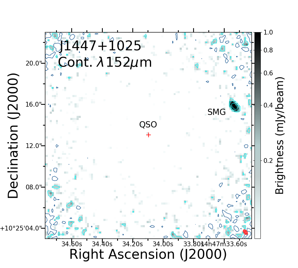
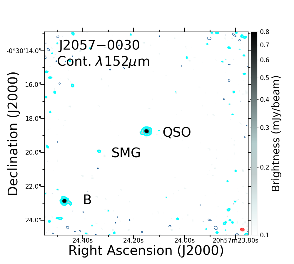
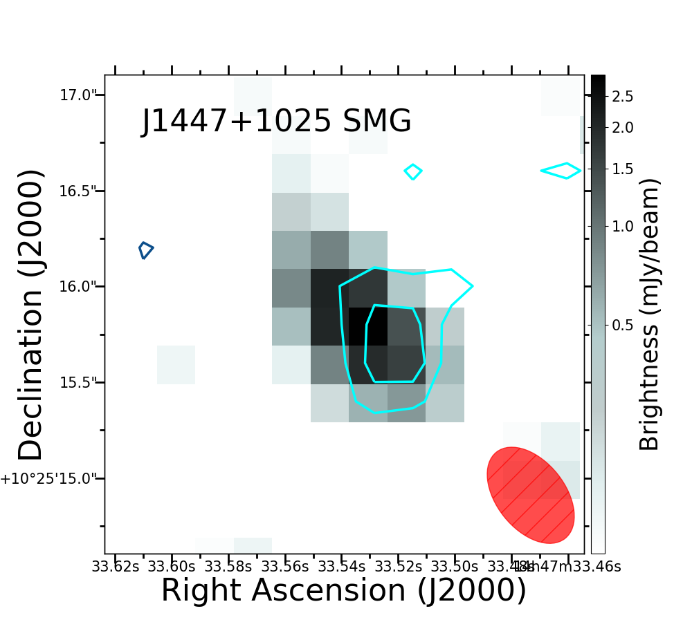
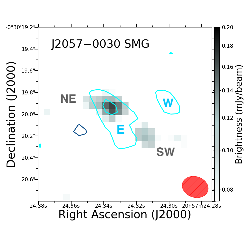
Figure 1: Top: Large-scale continuum images for the two FIR-faint quasars in our sample where companions have been found: J2057 and J1447. Note that J1447 is not detected in dust continuum. The gray-scale maps show the continuum emission determined from the line-free ALMA spectral windows. Cyan and blue contours trace emission levels at different positive and negative significance levels, respectively, with the first contour tracing the region where the continuum emission exceeds 2$\sigma$, and consecutive contours plotted in steps of $2\sigma$. The ALMA beams are shown as red ellipses near the bottom-right of each panel. Physical companions, i.e., sources that have clear [C ii] detections with redshifts consistent with those of the quasars, are marked as “SMG”. The continuum source accompanying J2057 that lacks significant [C ii] emission is marked as “B”. Bottom: Small-scale continuum and [C ii] line emission maps derived for the SMGs accompanying J1447 and J2057. For each source, the gray-scale map traces the continuum emission, while the contours trace the [C ii] line emission (i.e., surface brightness) at significance levels of 3 and 6$-\sigma$. For each source, the line fluxes used for the contours were extracted from a spectral window spanning $\pm 500\,{\rm km\,s}^{-1}$ around the [C ii] line peak. The ALMA beams are shown as red ellipses near the bottom-right of each panel. The two J2057 components observed in [C ii] emission are labeled E and W, while the two components seen in continuum are labeled NE and SW.

2.3 Data Reduction

Data reduction was performed using the CASA package version 4.7.2 (McMullin et al., 2007). CLEAN algorithms were ran with ”briggs” weighting and a robustness parameter of 0.5 in order to create continuum and emission line images. Continuum emission images were constructed using the line-free spectral window pair, while the UVCONTSUB command was used to subtract continuum emission from the [C ii] window pair, resulting in continuum-subtracted cubes. Observed flux densities and beam deconvolved continuum source sizes are presented in Table 2.

Sizes of the continuum emitting regions were determined from the respective images by fitting spatial 2D Gaussians to the sources, which are characterized by a peak flux, semi-major and semi-minor axes, and a position angle. The fluxes were measured by integrating over these spatial 2D Gaussians. The SMG companion to J2057 (see Section 2.4), however, seems to be composed of two separate sources which were not properly fitted by the CASA 2D Gaussian routine. Instead, sizes were obtained directly from the continuum images using an azimuthally averaged Gaussian fit. Since these values are not beam-corrected, they are quoted as upper limits in Table 2.

Various IMMOMENTS commands gave the velocity fields and velocity dispersion maps (first and second moment, respectively) from the [C ii] continuum subtracted cubes. To measure the properties of the $\left[{\rm C}\,\textsc{ii}\right]$ emission lines, we used both a ”spatial” and ”spectral” method. In the ”spatial” approach, we created zero-moment images (i.e., integrated over the spectral axis) for all sources and fitted the spatial distribution of line emission with 2D Gaussian profiles. Line fluxes were obtained as described before for the continuum flux determinations.

Table 2: Spectral Measurements

Subsample	Target		Cont. Flux	$\nu$	Cont. Size	$F_{\left[{\rm C}\,\textsc{ii}\right]}$	FWHM${}_{\left[{\rm C}\,\textsc{ii}\right]}$	$\nu_{0,\left[{\rm C}\,\textsc{ii}\right]}$	[C ii] size	$L_{\left[{\rm C}\,\textsc{ii}\right]}$	$\Delta d$	$\Delta v$
	ID	comp.	[mJy]	[GHz]	[′′]	[Jy km s-1]	[km s-1]	[GHz]	”	[$10^{9}\,L_{\odot}$]	[kpc]	[km s-1]
Bright	J0807	QSO	6.80 $\pm$ 0.20	334.87	0.23 $\times$ 0.19	5.8 $\pm$ 1.40	398.6 $\pm$ 19.2	323.27 $\pm$ 0.010	0.52 $\times$ 0.14	4.01	. . .	. . .
	J1404	QSO	11.31 $\pm$ 0.27	333.86	0.28 $\times$ 0.25	5.81 $\pm$ 0.71	483.3 $\pm$ 21.3	320.86 $\pm$ 0.009	0.52 $\times$ 0.43	4.08	. . .	. . .
	J1433	QSO	7.61 $\pm$ 0.33	334.05	0.32 $\times$ 0.26	4.79 $\pm$ 0.38	397.0 $\pm$ 13.7	331.78 $\pm$ 0.006	0.43 $\times$ 0.37	3.17	. . .	. . .
	J1616	QSO	6.29 $\pm$ 0.28	335.74	0.23 $\times$ 0.16	10.1 $\pm$ 1.50	469.5 $\pm$ 24.1	322.99 $\pm$ 0.011	0.60 $\times$ 0.36	7.00	. . .	. . .
	J1654	QSO	4.73 $\pm$ 0.10	344.53	0.10 $\times$ 0.08	2.07 $\pm$ 0.46	543.0 $\pm$ 34.9	331.81 $\pm$ 0.016	0.31 $\times$ 0.08	1.36	. . .	. . .
	J2225	QSO	13.13 $\pm$ 0.21	334.61	0.22 $\times$ 0.17	8.05 $\pm$ 0.73	445.5 $\pm$ 22.4	322.50 $\pm$ 0.010	0.44 $\times$ 0.29	5.60	. . .	. . .
Faint	J1017	QSO	1.36 $\pm$ 0.10	331.76	0.23 $\times$ 0.20	1.93 $\pm$ 0.27	223.8 $\pm$ 8.3	319.49 $\pm$ 0.004	0.32 $\times$ 0.30	1.37	. . .	. . .
	J1151	QSO	$<0.81$	346.13	. . .	$<0.31$	. . .	. . .	. . .	. . .	. . .	. . .
	J1321	QSO	1.56 $\pm$ 0.07	343.73	0.29 $\times$ 0.22	1.72 $\pm$ 0.21	480.7 $\pm$ 26.4	322.12 $\pm$ 0.012	0.46 $\times$ 0.27	1.13	. . .	. . .
	J1447	QSO	$<0.12$	346.61	. . .	0.14 $\pm$ 0.09	293.2 $\pm$ 113.6	334.50 $\pm$ 0.027	0.30 $\times$ 0.28	0.09	. . .	. . .
	J1447	SMG	3.86 $\pm$ 0.17	346.61	0.40 $\times$ 0.15	0.88 $\pm$ 0.27	215 $\pm$ 22	334.37 $\pm$ 0.008	$<0.3$	0.57	59	206.5
	J1447	SMG				0.54 $\pm$ 0.16	199 $\pm$ 33	333.72 $\pm$ 0.008	$<0.3$	0.35	59	701.2
	J2057	QSO	2.03 $\pm$ 0.14	346.52	0.24 $\times$ 0.21	2.51 $\pm$ 0.31	331.4 $\pm$ 20.5	334.44 $\pm$ 0.009	0.40 $\times$ 0.18	1.63	. . .	. . .
	J2057	SMG NE,E	0.28 $\pm$ 0.04	346.52	$<0.3$	0.63 $\pm$ 0.11	475.4 $\pm$ 84	334.62 $\pm$ 0.009	$<0.3$	0.41	20	-161.4
	J2057	SMG SW,W	0.17 $\pm$ 0.06	346.52	$<0.3$	0.37 $\pm$ 0.07	336.3 $\pm$ 68	334.32 $\pm$ 0.009	0.57 $\times$ 0.14	0.24	20	107.7
	J2244	QSO	3.34 $\pm$ 0.09	346.95	0.20 $\times$ 0.19	3.86 $\pm$ 0.29	283.1 $\pm$ 7.4	335.71 $\pm$ 0.003	0.40 $\times$ 0.30	2.49	. . .	. . .

In the ”spectral” approach, we extracted 1D spectra from the $\left[{\rm C}\,\textsc{ii}\right]\$ continuum subtracted cubes. A Gaussian profile was fitted to the emission line profiles, from which we obtained the integrated line flux.

We found that the two different methods described above to be in good agreement, with a median difference of 0.05 dex. As stated in T17 the ”spatial” approach is less sensitive to the low Signal-to-Noise (S/N) outer regions of the sources and the low S/N ”wings” of the line profiles, thus we adopt this method for our own analysis. J2057, however, has a spectral gap (as described in 2.2) lying in the center of the [C ii] line. This proved difficult for the ”spatial” method as no interpolation of the missing line flux was possible. Hence, the line flux reported in Table 2 was obtained with the ”spectral” approach. Also, both SMG companions to J1447 and J2057 (see next Section) show separate dynamical components. In the case of J1447 the ”spectral” approach was used to determine their properties. The J2057 SMG also breaks into two components in continuum emission, which are not clearly related to the [C ii] emission. Both components are characterized in Table 2.

2.4 Source Detections

Ten of our twelve new quasars are clearly detected in both continuum and $\left[{\rm C}\,\textsc{ii}\right]$ emission with 6-12$\sigma$ significance. While J1447 is only detected at a 3$\sigma$ level in $\left[{\rm C}\,\textsc{ii}\right]$ line, and J1151 is not detected at all. J1447 and J1151 are both FIR-faint sources. Because J1447 has a very weak signal, it was not possible to fit a Gaussian to the spatial distribution of its line and continuum emission. Instead, ‘aperture’ photometry was carried out with an area corresponding to roughly the beam size. The [C ii] emission of J1447 was found to have a S/N $\sim$ 3.6, while there was a non-significant signal in the continuum. The continuum values listed in Table 2 for J1447 and J1151 correspond to 3 times the average RMS noise about the expected quasar positions.

Two FIR-faint quasars show the presence of companions detected in both continuum and [C ii] emission with a significance of 6-9 $\sigma$. Continuum maps for these two sources are presented in Figure 1. A continuum-only source is found separated from J2057 by $6\farcs 3$ in the SE direction, which corresponds 41.8 kpc at the redshift of the quasar and is marked with a ’B’ in Figure 1. We can put a lower limit of $\sim\pm 1500$ km s^-1 to the velocity shift of any [C ii] emission from this source and the [C ii] emission from the quasar host. Because of the separation and lack of a $\left[{\rm C}\,\textsc{ii}\right]$ line detection, we conclude that this continuum source is most likely a source only seen in projection. A similar continuum-only source is found in T17, which is concluded to be a background/foreground projection. Information about companions can be found in Tables 1 and 2.

For all our quasars detected in both, continuum and [C ii], the two emissions follow each other well. The exceptions are the two detected SMGs. Their detailed continuum and [C ii] maps are presented in Figure 1. In the case of J1447, the continuum emission seems more extended towards the north than the [C ii] emission, although weaker, redshifted [C ii] emission appears towards the north in dynamical maps (see next Section). The SMG to J2057 has secondary peaks in [C ii] and continuum emission. These are labeled as E, W and NE, SW in Figure 1, respectively. We will see in the next Section that there is strong indication of gravitational perturbations in these two SMG sources.

	FIR-Bright Objs.
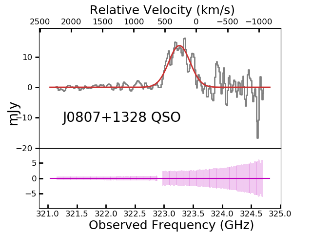
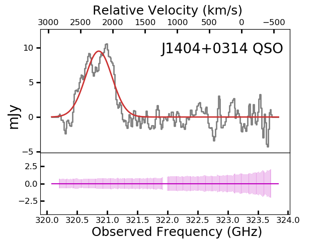
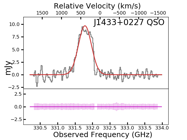
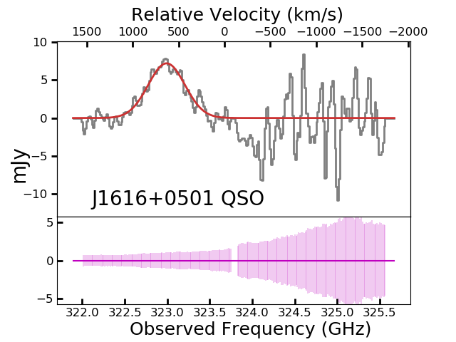
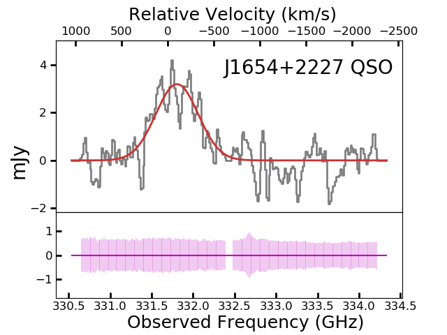
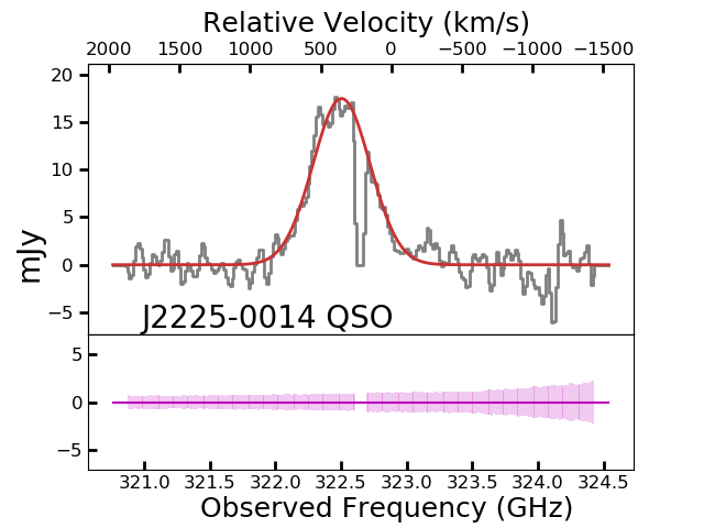
	FIR-Faint Objs.
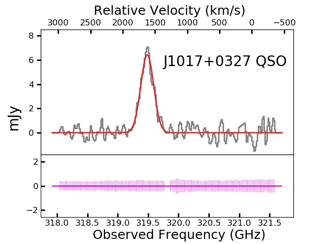
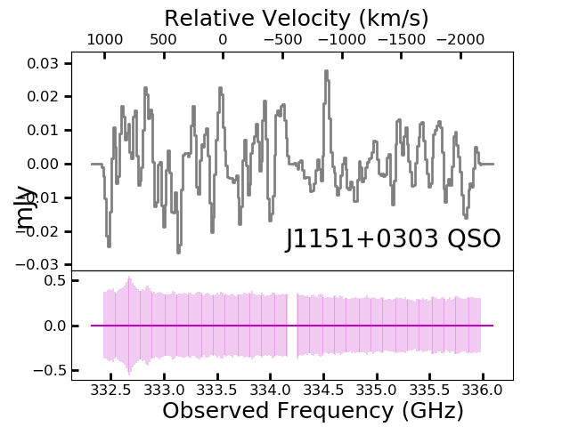
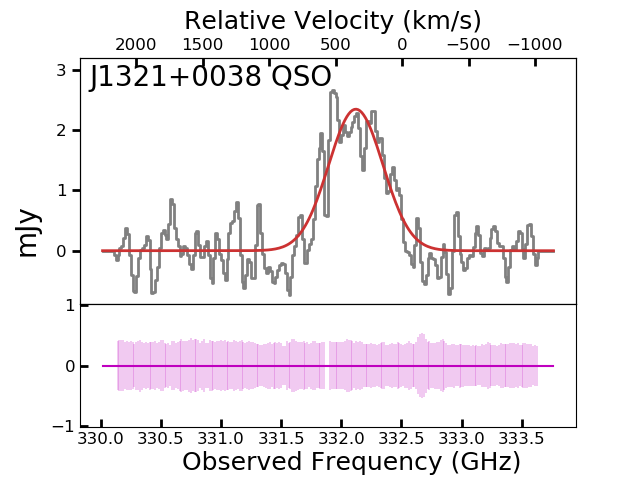
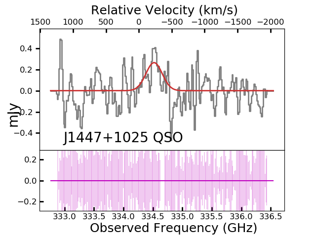
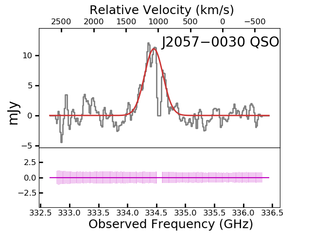
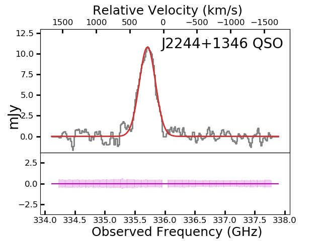
	SMGs

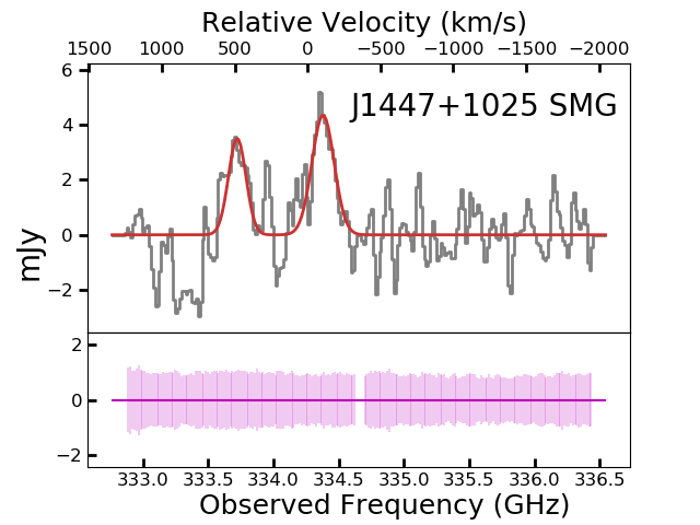
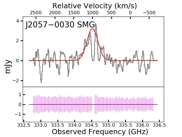
Figure 2: Spectra of the [C ii] $\lambda 157.74\,\mu{\rm m}$ emission line for all the new ALMA observations reported in this work. FIR-bright sources are presented in the top two rows, FIR-faint sources in the middle two rows, and accompanying SMGs are presented in the bottom row. For each spectrum the upper x-axis denote the velocity offsets with respect to the redshift derived from the Mg ii broad emission lines (T11). Red lines show the Gaussian fits to the line profiles. RMS spectra are also included in the same scale as the flux spectrum except for J1151 where there is no [C ii] detection.

FIR-Bright Objs.


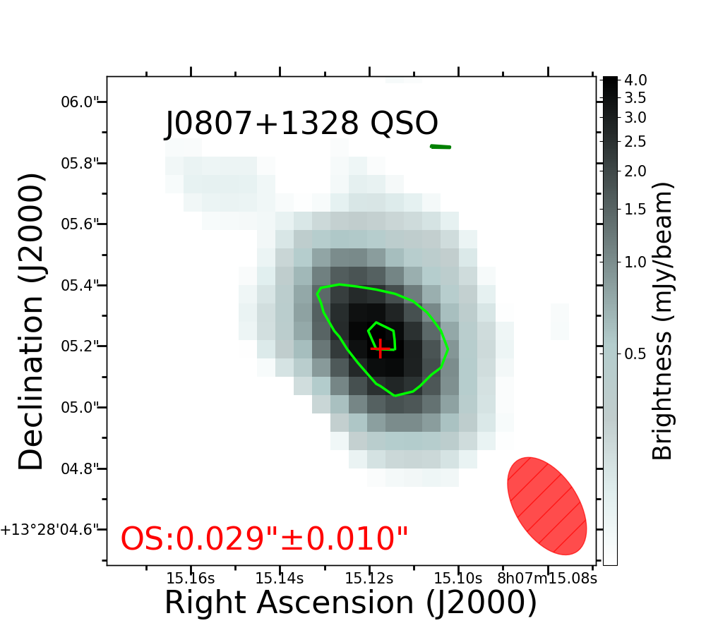
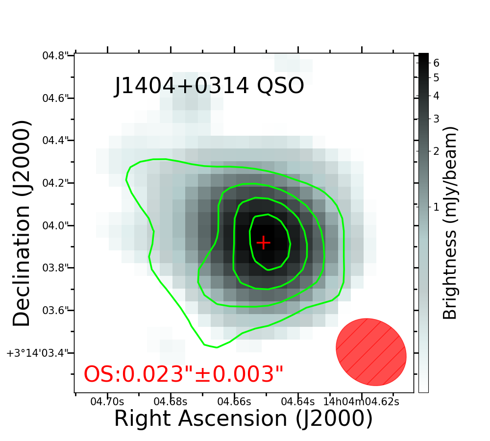
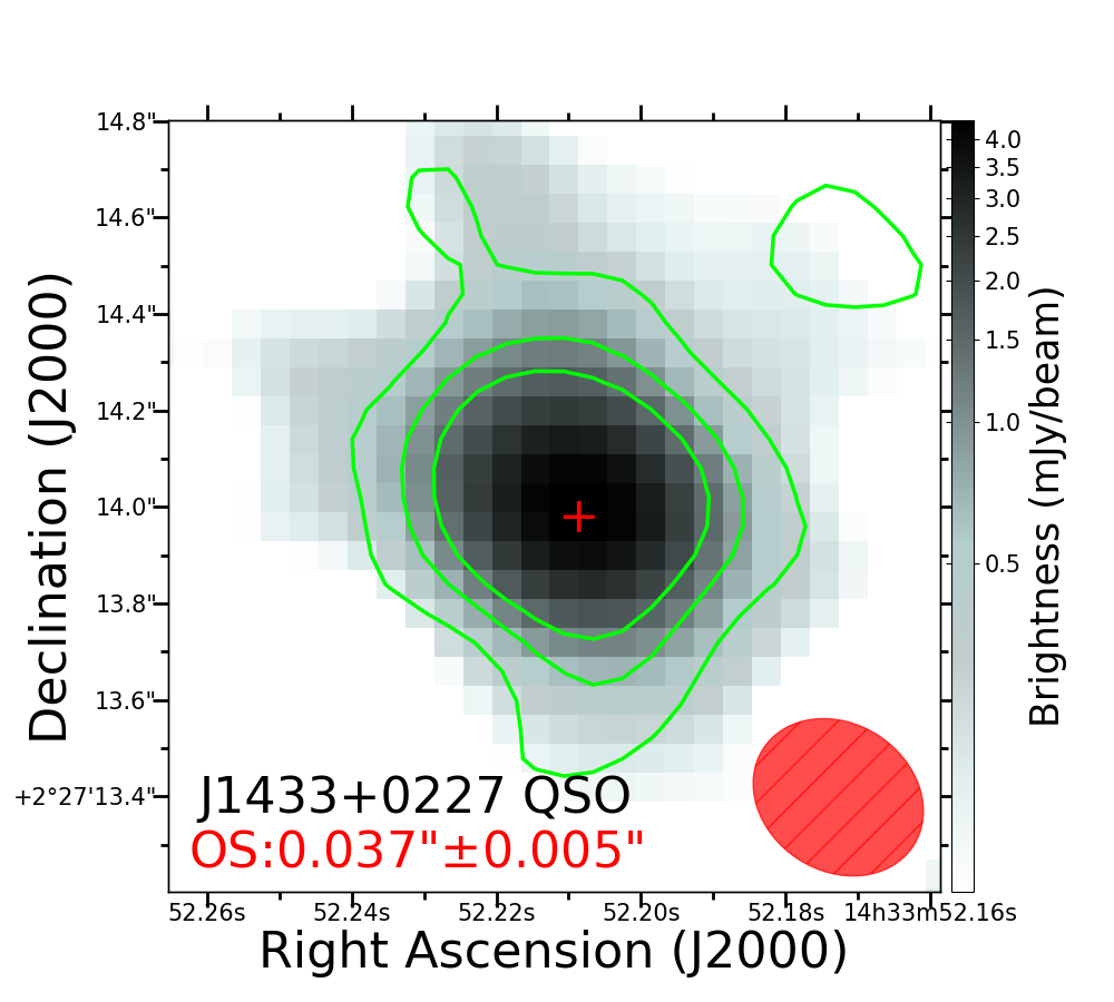
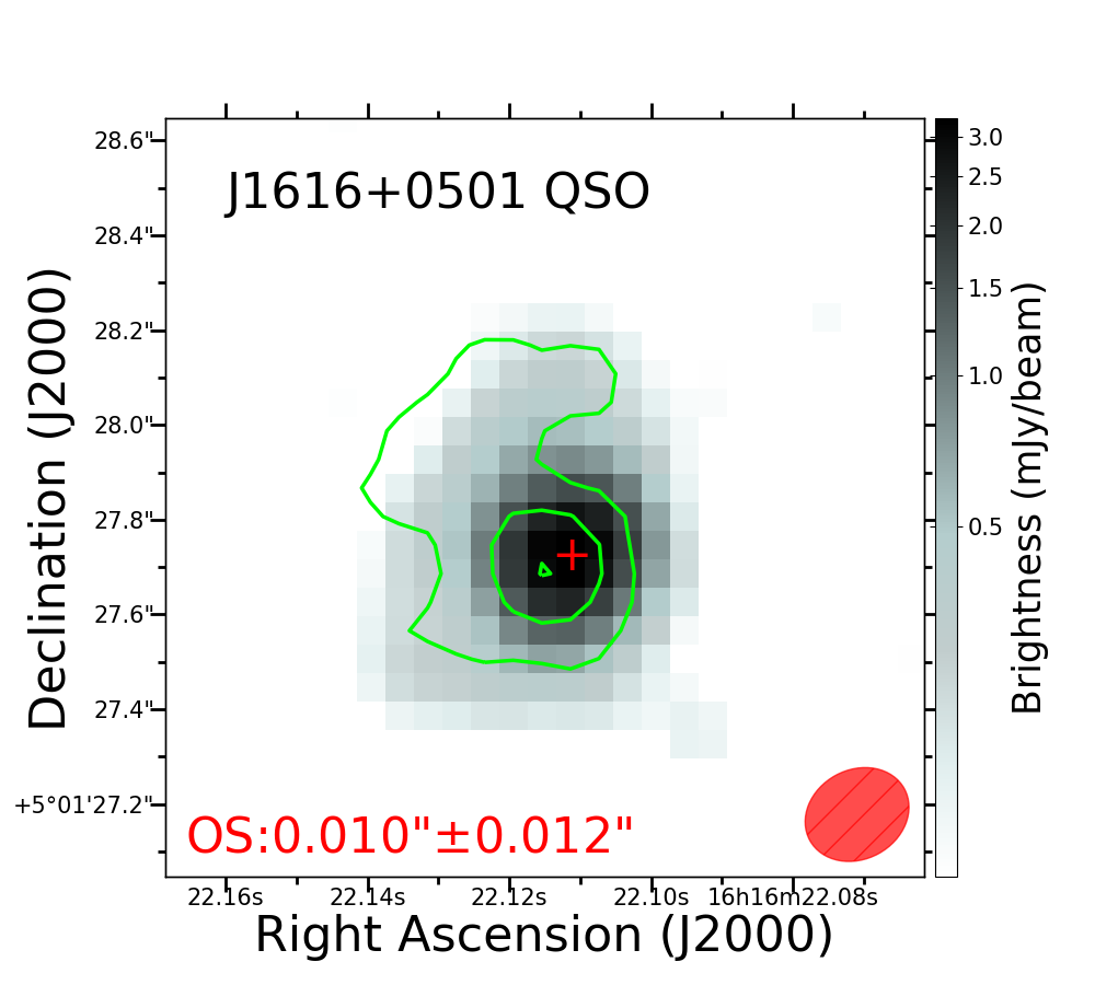
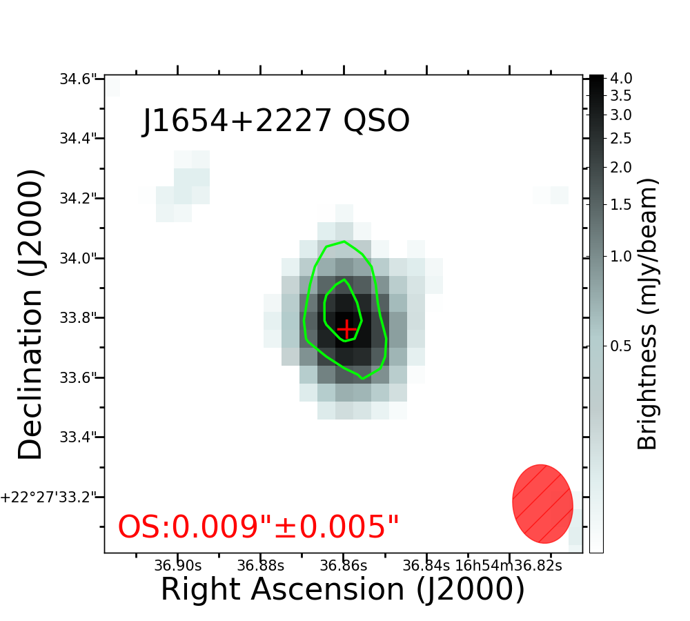
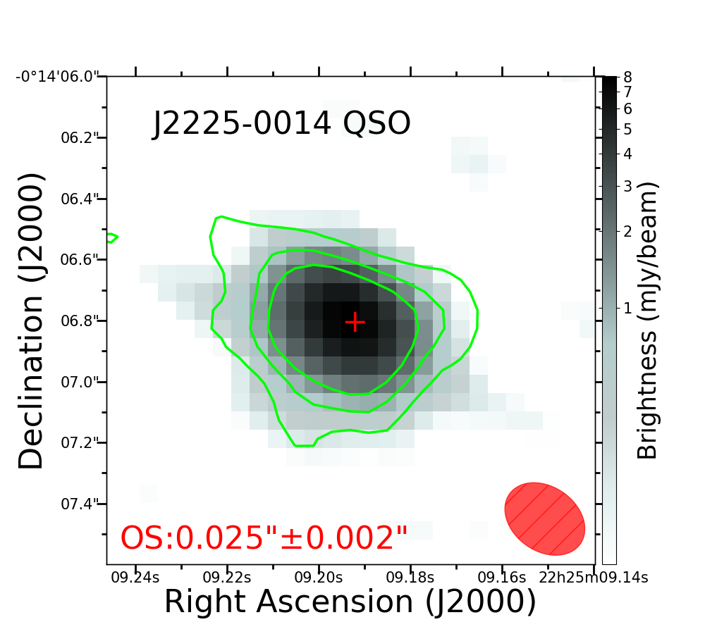
FIR-Faint Objs.

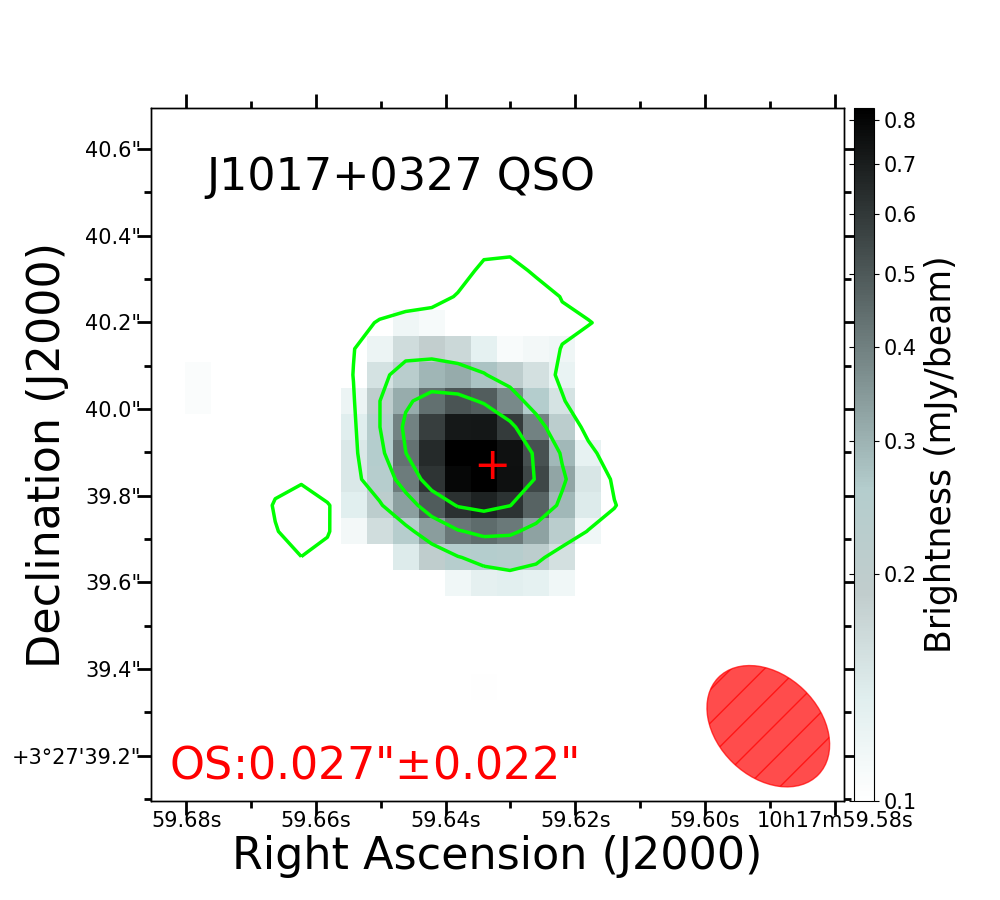
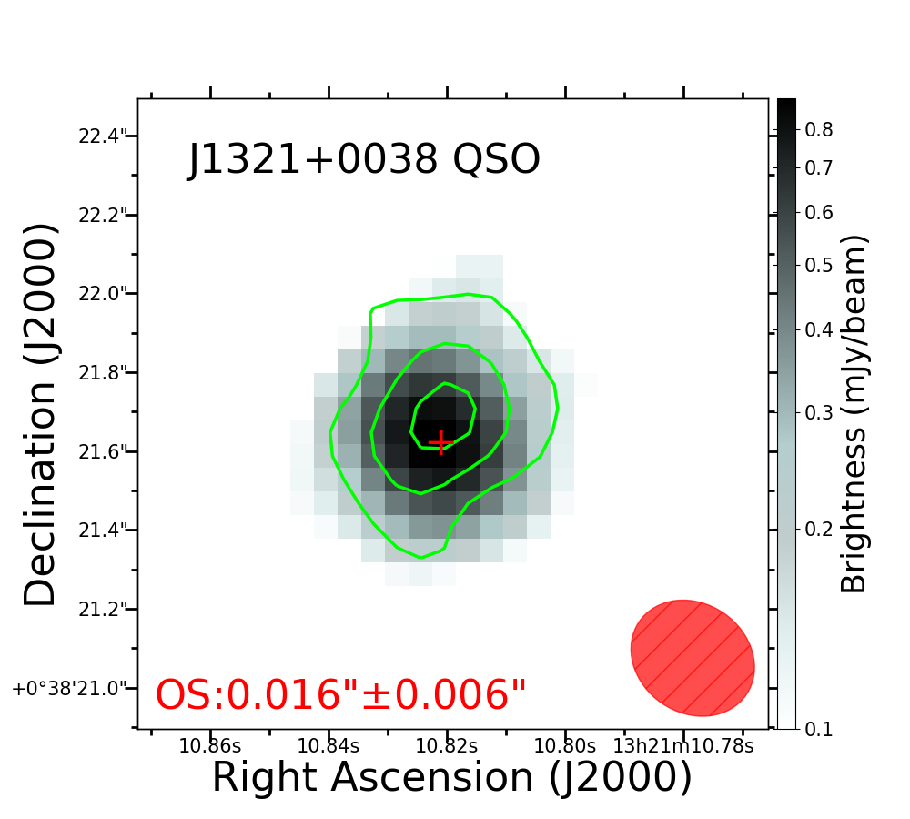
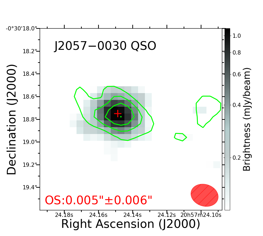
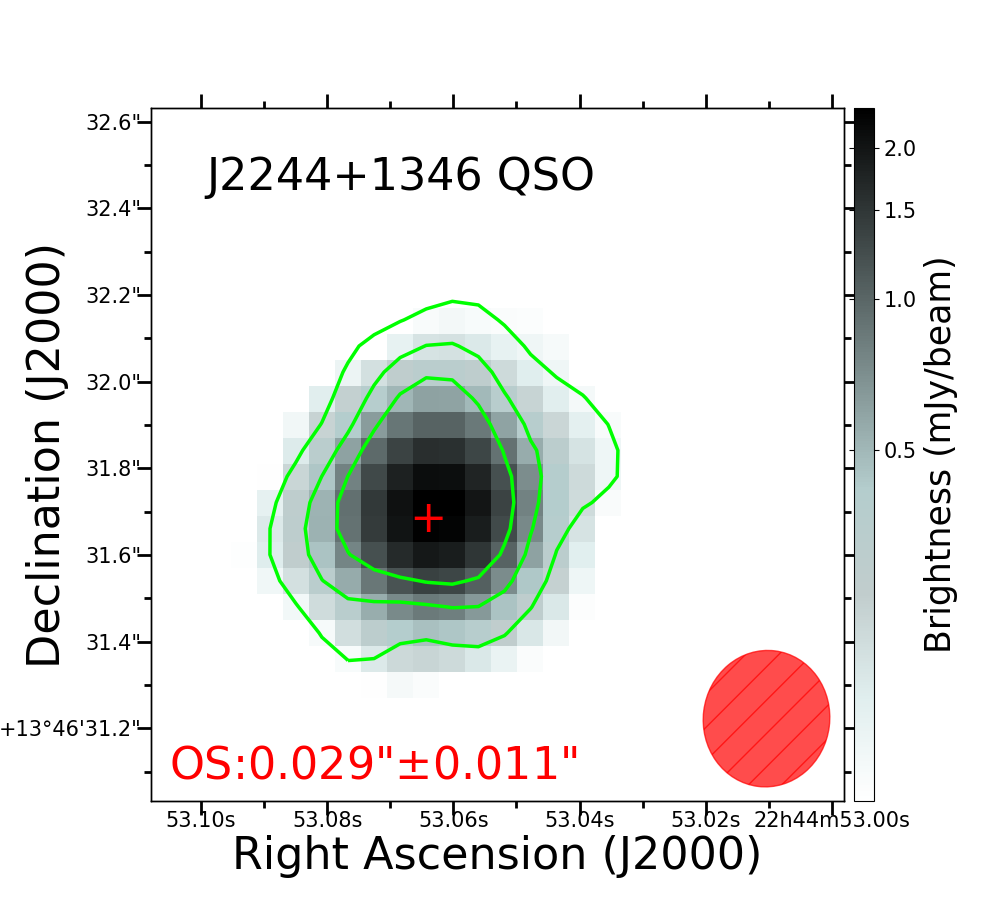
Figure 3: Small-scale continuum and [C ii] line emission maps derived from the Cycle-6 ALMA data, for all the sources with clear detection of [C ii] line emission. The FIR-bright sources in our sample are the top two rows, the FIR-faint sources are the bottom two rows. For each source, the gray-scale map traces the continuum emission, while the contours trace the [C ii] line emission (i.e., surface brightness) at significance levels of 3, 6, 9, and 12$-\sigma$. For each source, the line fluxes used for the contours were extracted from a spectral window spanning $\pm 500$ km s^-1 around the [C ii] line peak. The ALMA beams are shown as red ellipses near the bottom-right of each panel. The optical position from GAIA is marked with a red cross (+). In the bottom left of each image we list the Optical Separation (OS) along with the associated error.

FIR-Bright Objs.


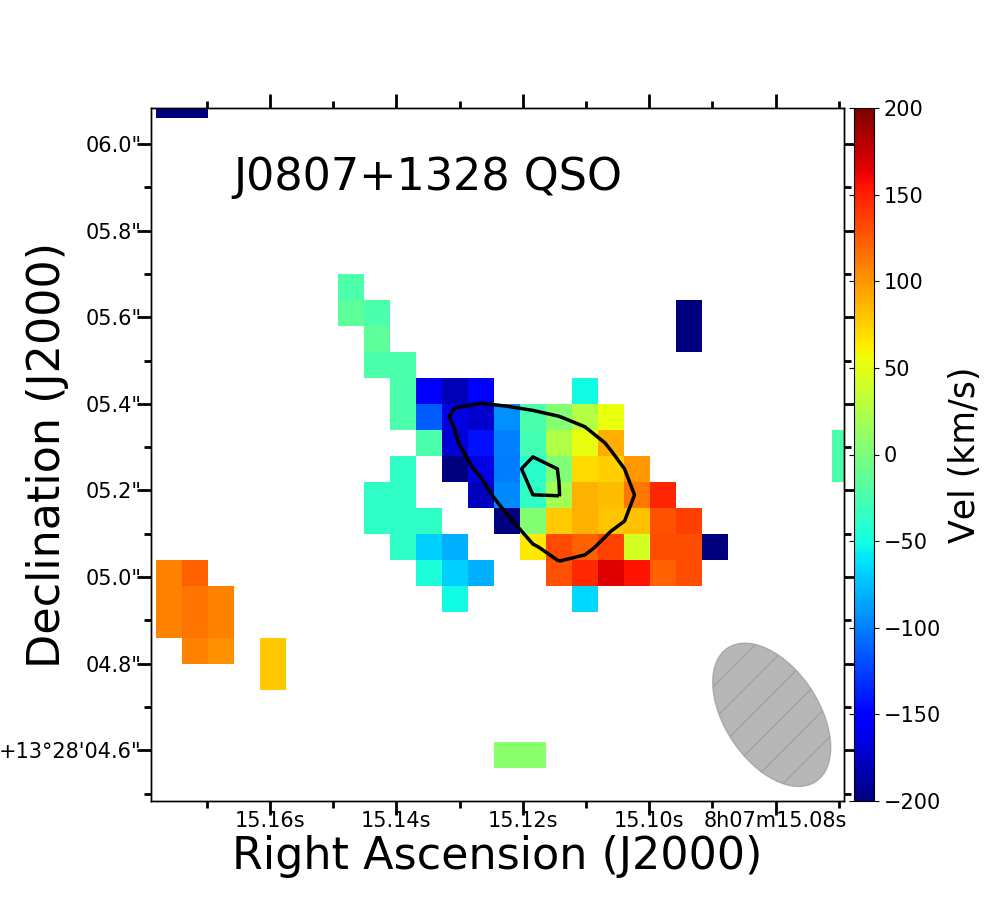
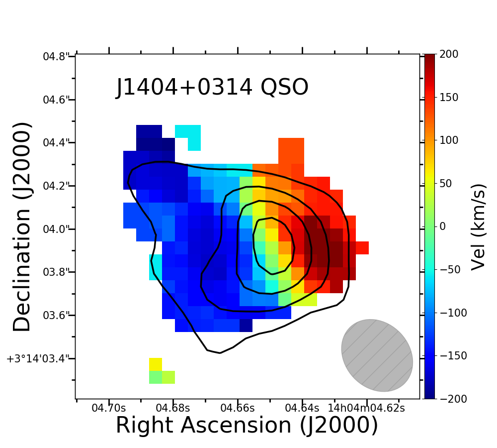
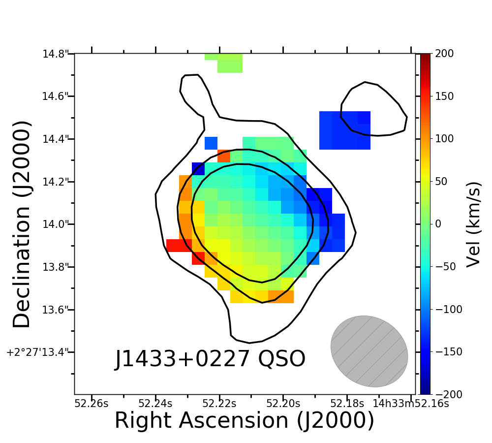
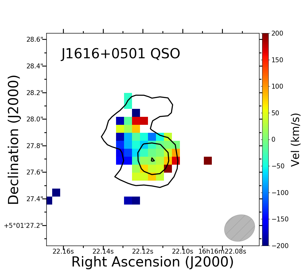
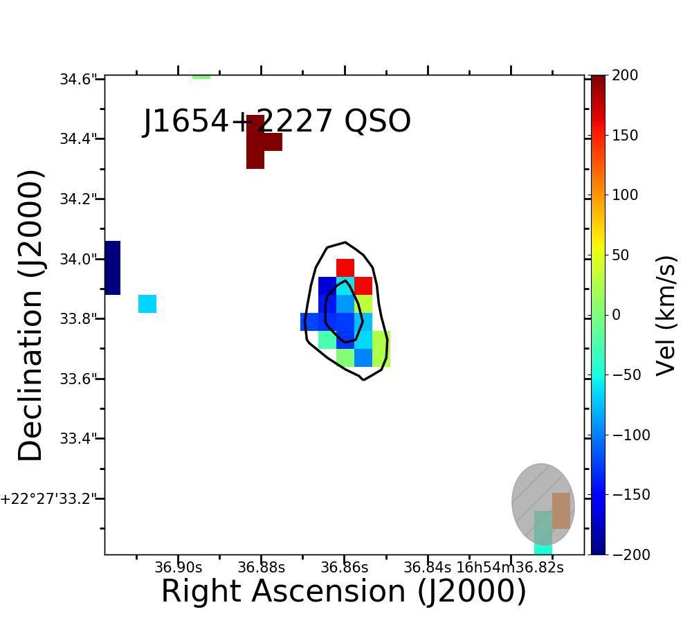
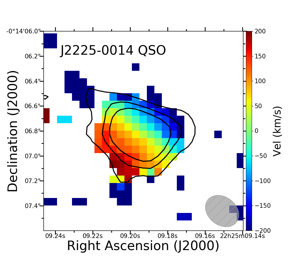
FIR-Faint Objs.


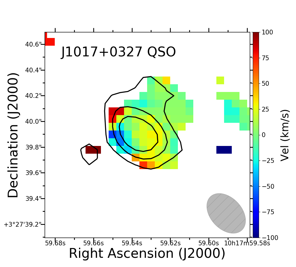
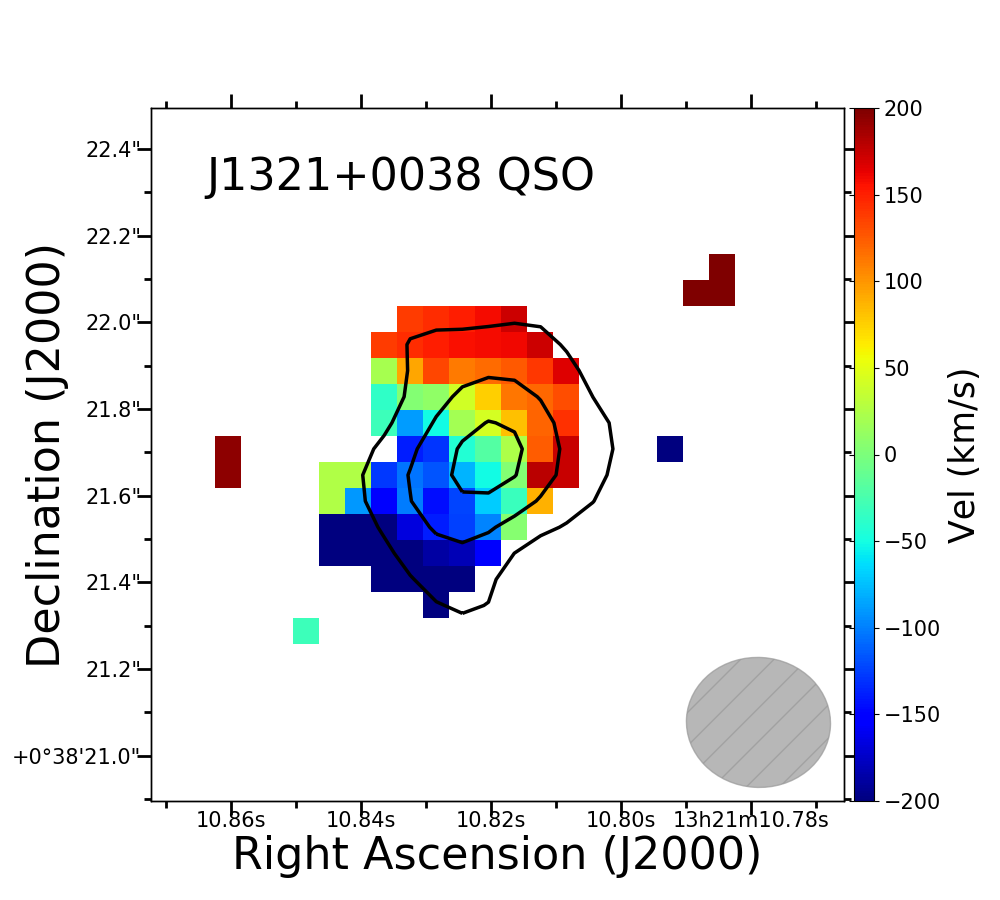
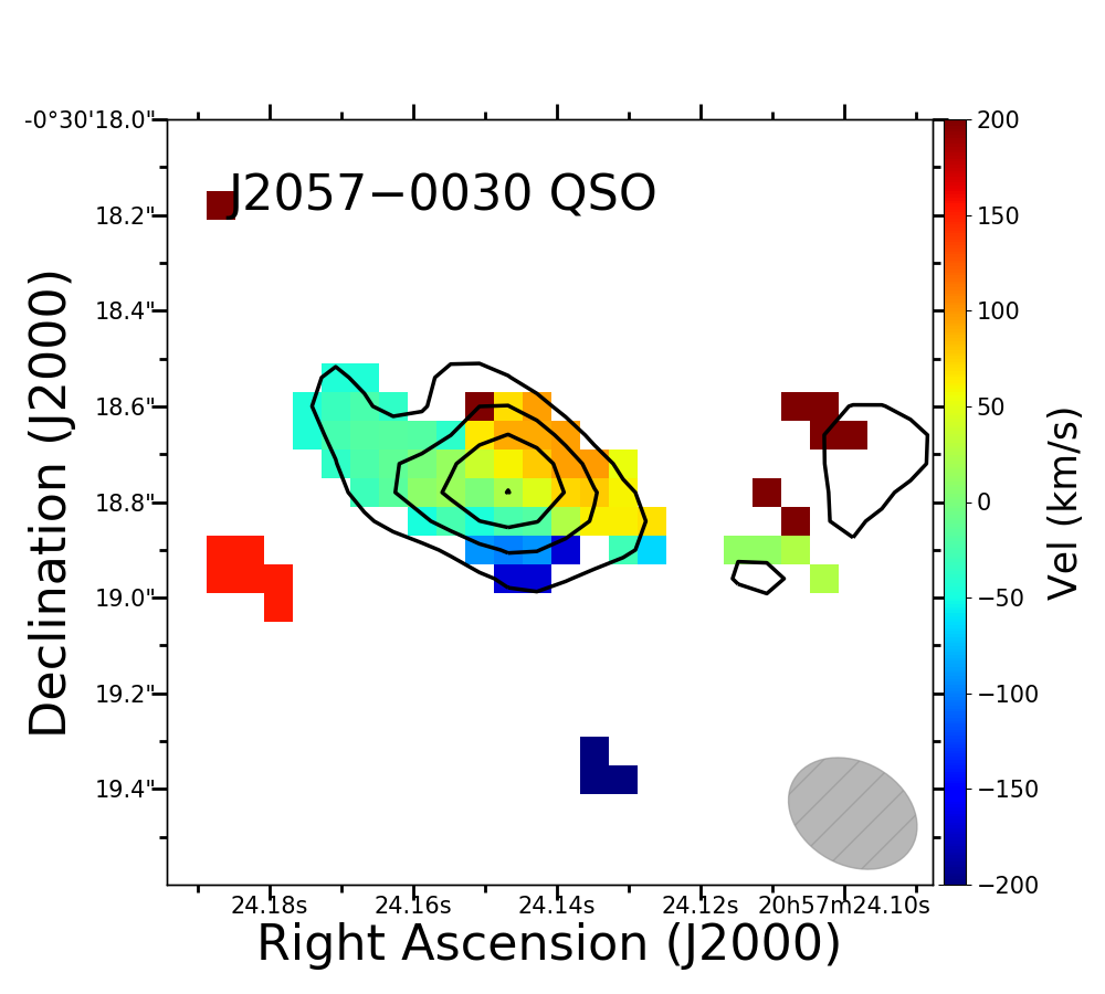
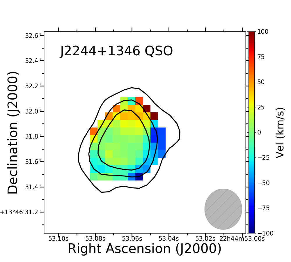
SMGs

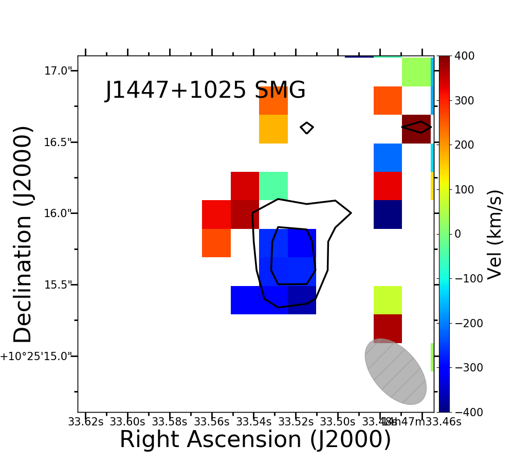
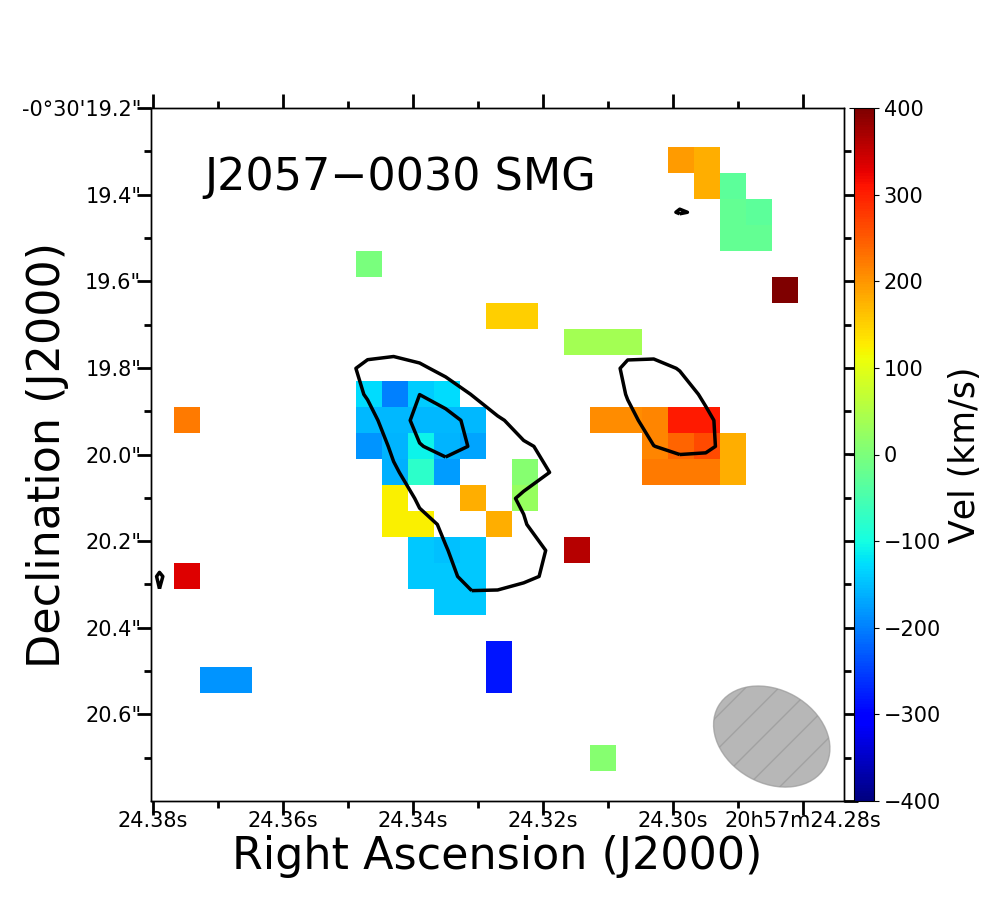
Figure 4: [C ii] velocity maps for the FIR-bright sources in our sample (top two rows), FIR-faint sources (middle two rows), and the companion SMGs (bottom row). Black contours trace the [C ii] emission line surface brightness at significance levels of 3, 6, 9, and 12$-\sigma$. The ALMA beams are shown as hatched gray ellipses near the bottom-right of each panel.

2.5 [C ii] Line Properties

In Figure 2, we plot the continuum subtracted [C ii] spectral region for all 12 quasar hosts presented in this work, including J1151 which was undetected in both continuum and [C ii], and J1447 which had a 2$\sigma$ level detection in [C ii]. We also include spectra for two SMGs accompanying J2057 and J1447. A best-fit line model using a Gaussian profile is overlaid. The Root Mean Square (RMS) spectra is plotted below each emission line spectra.

Figure 4 shows velocity maps for the ten quasar hosts significantly detected in [C ii] and the two SMGs accompanying J1447 and J2057. The weak [C ii] emission from J1447 was not sufficient to determine moment maps. The morphologies of our targets are not as uniform as in T17, possibly due to some of our sources being observed through spectral sub-mm windows with worse transmission, as mentioned in Section 2.2. Well behaved velocity maps, with a clear velocity gradient across the system, which suggests rotation of a flat gaseous structure, is only seen in about half of systems. The remaining sources show noisier, more irregular maps, although evidence for a velocity gradient is still present.

As in T17, some of our quasar hosts show increased velocity dispersions in the centers of the [C ii] - emitting regions, with $\sigma_{v}\sim 100\ {\rm km\,s}^{-1}$, which can be an indication of beam smearing. This could lead us to overestimate the rotation kinematics we see in Figure 4. However we do not expand on correcting this smearing as other studies of sub-mm sources have done, as our targets are only partially resolved and modeling the rotation is not possible. In fact, as many of our sources do not exhibit clear rotation dominated kinematics (e.g., J1017 and J1654), other factors could be affecting the kinematics of our hosts. Possible alternatives such as a turbulent component have been demonstrated in several recent studies of resolved ISM kinematics in high-redshift galaxies (e.g., Gnerucci et al., 2011; Williams et al., 2014).

The majority of our objects have a single peak line profile except for J1404 which exhibits double peak emission in the [C ii] line, and the SMG companion to J1447. The double feature seen in J1404 has two peaks separated $\sim 350$ km s^-1 from each other, while the SMG of J1447 shows two components to the [C ii] line separated by $\sim 600$ km s^-1.

The velocity map of J1404 in Figure 4 shows a single source with strong rotational signatures and a large total velocity amplitude of $\sim 400\,{\rm km\,s}^{-1}$, roughly the same separation we see in the spectrum. This FIR-bright source does not show the presence of companions, but the double peak could signal the late evolutionary stage of a merger event.

On the other hand, the double feature seen in the SMG of J1447 most likely corresponds to a double source. This is seen in the bottom right panel of Figure 4 where two spatially separated kinematic components appear. The north-east peak is rather weak, as it is below the 3 $\sigma$ threshold of the [C ii] contours, but it is clearly recovered in the spectrum shown in Figure 2 and coincides with strong emission seen in dust continuum (see Figure 1).

Finally, J2057 also presents some interesting dynamical features. Besides the presence of two dust continuum peaks and a complex velocity map shown by the companion SMG, the quasar itself shows strong evidence for dynamical disruption: its [C ii] emission appears as consistent with a $\sim 100\,{\rm km\,s}^{-1}$ rotating disk plus debris material and a $\sim 20$ kpc-long collimated ‘tadpole-like’ structure orientated roughly in the E-W direction, which is constrained to a very narrow velocity range. This structure is not apparent in Figure 4 because of the velocity binning. J2057 and its SMG companion will be the subject of a future paper.

2.6 Optical Center Separation

In Figure 3 we plot the continuum maps of our quasars, along [C ii] emission contours. From The 2nd data release of the Gaia mission (Gaia Collaboration et al., 2018a), crossed referenced with the Pan-STARRS 1 data base (Flewelling et al., 2016), we obtain the optical centers of our objects.

We then compute Optical Separation (OS) as the separation between the Gaia optical center and the peak of the dust continuum emission from our ALMA data, as determined by Gaussian fits in Section 2.3. Each image in Figure 3 lists the OS along with the associated error. OS values have a range of 0.005” - 0.062” for our entire sample. The median positional uncertainty of quasars in DR2 of Gaia is 0.4 milli-arcsecond (Gaia Collaboration et al., 2018b), while those objects which are cross referenced with the Pan-STARRS data base have median uncertainties of 3.1 and 4.8 milli-arcsecond for $\Delta ra$ and $\Delta dec$, respectively (Chambers et al., 2016). The associated error of our OS considers uncertainties associated with the optical position as well as our Gaussian fits to the continuum emission, giving an overall median error of $\sim$ 11 mas.

Offsets of the optical center could be an indicator of dual-AGN or late stage major mergers (Orosz & Frey, 2013; Makarov et al., 2017). However these studies found OS values on scales of hundreds of milli-arcsecond scales, much larger than what we see. We also see that there is no correlation between host galaxy velocity gradients and OS. J1328-0224 is our object with the highest OS (62 mas) in our sample, but Figure 4 shows that it has a very low gradient of velocity with rather uniform values. In contrast, J2057-0030 has the lowest OS but we believe it to be a perturbed system with a tidal tale. Thus we do not consider the OS to be an indicator of mergers or perturbations for our sources.

3 Results and Discussion

In what follows we divide the discussion into those results that are robust and do not rely on unconstrained assumptions and those that are more speculative and that need further observations in order to prove their veracity. In particular, the determination of gas and dynamical masses for our quasar hosts are highly uncertain, and therefore all discussion based on these determinations should be taken withe extra caution.

3.1 Main Findings

3.1.1 Emission Line Velocity Offsets

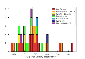
Figure 5: Histogram presenting the distribution of the velocity shifts of the Mg ii with respect to the [C ii] emission lines of the quasars. Our twelve observations and those presented in T17 are at $z\simeq 4.8$, while those in Venemans et al. (2016) and Willott et al. (2013, 2015, 2017) are at $z\gtrsim 6$. The [C ii] line is clearly redshifted with respect to the Mg ii measurements with a mean and standard deviation of $372\pm 582\,{\rm km\,s}^{-1}$. The vertical line denotes the median of 337 km s^-1.

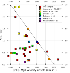
Figure 6: Eddington ratios of our compiled quasars against the observed Mg ii offsets. References for the Mg ii measurements and the Eddington ratios can be found in Table 6. The average Eddington Ratio is 0.83. We plot a line in black to help illustrate that there are no objects with both high Mg ii offsets and high Eddington ratios. 36 quasars are plotted in total. Only 5 of the 8 Decarli quasars have published Eddington ratios.

Neutral carbon has a low ionization potential (11.3 eV) and can be excited by electron collisions. Therefore, [C ii] emission can be found in the ISM throughout a galaxy, particularly tracing photo-dissociation regions, that is, naturally diffuse and partially ionized gas. Although from observations in the local universe it is seen that the [C ii] line is broader than molecular gas (e.g., Goicoechea et al. 2015), because of its high brightness and narrow intrinsic width it is a good measure of the systemic redshift of the quasar host galaxy. While the Mg ii line, produced in the vicinity of the SMBHs in the so called Broad Line Region (BLR), is dominated by the gravitational SMBH as well as other central bulk nuclear winds or turbulences. In Table 3 we compare the redshifts obtained from the [C ii] and Mg ii lines ($\Delta v_{{\rm Mg}\,\textsc{ii}}$) for our 17 quasar hosts with detected [C ii]. For unobscured AGN at moderate redshifts ($z<2$), the BLR Mg ii line is found within $\sim 200\$km s^-1 of the systemic redshifts (Richards et al., 2002; Shen et al., 2016; Mejía-Restrepo et al., 2016), and centered around $\sim 0$ km s^-1(see Figure 2 in Shen et al. 2016). The large dispersions in the line shifts are clearly due to the broad nature of the BLR lines and hence the difficulties in determining precise line centers.

For comparison, we also list the SDSS-based redshift determinations published in Hewett & Wild (2010), along with the difference with respect to the [C ii] line ($\Delta v_{SDSS}$). At $z\sim 5$ SDSS-based redshifts would be determined using the BLR UV Ly$\alpha$, S iv and C iv emission lines, which are usually considered problematic because of the absorbed Ly$\alpha$ profile, the weakness of the S iv line, and the well established blueshifts present in the C iv line. In fact, we see no correlation between $\Delta v_{SDSS}$ and $\Delta v_{{\rm Mg}\,\textsc{ii}}$, most likely because of the uncertainties associated to the $z_{SDSS}$ determinations (Mason et al., 2017; Dix et al., 2020).

From table 3 we can see that most objects in our total sample of 17 quasar hosts have significant blueshifts of the Mg ii line with respect to the [C ii] line ($\Delta v_{{\rm Mg}\,\textsc{ii}}>0$). The average value for $\Delta v_{{\rm Mg}\,\textsc{ii}}$ is 464 km s^-1, with a standard deviation of 657 km s^-1while the median is found to be at 379 km s^-1. As Venemans et al. (2016) already pointed out, since the distribution of offsets is not centered around 0 km s^-1, we can assume that they are not due to the uncertainty associated with fitting the broad emission line of Mg ii. This is further supported by Shen et al. (2016), where they state that the intrinsic uncertainty of using the Mg ii broad-line for estimating redshifts is 200 km s^-1, smaller than our median offset. We find no noticeable correlation between Mg ii offsets and the presence of companions.

Venemans et al. (2016) compiled a list of $z>6$ quasars and compared the redshift measurements from the ${\rm Mg}\,\textsc{ii}$ line and those of the CO molecular line or the [C ii] atomic line. The median of the $z_{\rm\left[{\rm C}\,\textsc{ii}\right]/CO}-z_{{\rm Mg}\,\textsc{ii}}$ distribution for their sample is 467 km s^-1 with a standard deviation of 630 km s^-1, almost identical to our findings. We created our own compilation, but used exclusively quasars with a measured $\left[{\rm C}\,\textsc{ii}\right]$ line for the sake of congruity. The compilation is populated by our total sample of 17 quasars, eight quasars taken from Decarli et al. (2018), five quasars found in Willott et al. (2013, 2015, 2017), five quasars from Venemans et al. (2012, 2016, 2017), two from Mazzucchelli et al. (2017), and one each from Banados et al. (2015) and Wang et al. (2016). We present the Mg ii offsets of this compilation as a histogram in Figure 5 and in Table 6. For this compilation we found a mean $z_{\left[{\rm C}\,\textsc{ii}\right]}-z_{{\rm Mg}\,\textsc{ii}}$ of 372 km s^-1, a median of 337 km s^-1, and a standard deviation of 582 km s^-1. It should be noted that only our sample is at $z\simeq 5$, while the quasars from the literature are all at $z\gtrsim 6$. The mean and median of the $z\gtrsim 6$ only quasars are 300 and 309 km s^-1, respectively, very close to the results from our full compilation. This result strongly suggests a velocity difference between the BLR and quasar host galaxies of several hundred km s^-1.

Blueshifts are usually associated to outflowing gas which is approaching the observer. Blueshifts seen in the C iv line, for example, are usually interpreted as evidence for nuclear outflows and they seem to correlate well with accretion rate (Coatman et al., 2016; Sulentic et al., 2017; Vietri et al., 2018; Sun et al., 2018; Ge et al., 2019). We have looked for such correlation for the objects in our compilation and found none. Figure 6 presents the accretion rate in units of Eddington (as reported in the literature) versus the measured [C ii]-Mg ii shifts. A rather low correlation coefficient is determined, with $r=-0.23$. In fact, Figure 6 suggests that low accretion sources can show a wide range of possible shifts, while high-Eddington sources tend to show small offsets, if any. We also tested a correlation of the offsets with infrared luminosities (compiled values can also be found in Table 6) but no significant result was found ($r=0.26$).

Like in Section 2.6 we search for correlations with the presence of companions. On average the mean offset of objects with companions is lower than the entire sample (92.4 km s^-1). Interestingly, of the four quasars with companions presented in Decarli et al. (2018), two have tabulated [C ii]-Mg ii offsets in Table 6, giving a mean offset of $\sim 0$ km s^-1. Since the number of sources with companions is very small, these are by no means conclusive findings, but suggest a possible link between merger activity and smaller [C ii]-Mg ii shifts.

Table 3: Redshifts and $\left[{\rm C}\,\textsc{ii}\right]$ Line Shifts

Sub-	Target	$z_{\left[{\rm C}\,\textsc{ii}\right]}$	$z_{SDSS}$	$\Delta v_{SDSS}$	$z_{{\rm Mg}\,\textsc{ii}}\tablenotemark{a}$	$\Delta v_{{\rm Mg}\,\textsc{ii}}$
sample				km s-1		km s-1
Bright	J0807	4.879	4.871	$+$378	4.874	$+$256
	J1404	4.923	4.871	$+$2208	4.880	$+$2208
	J1433	4.728	4.685	$+$2281	4.721	$+$379
	J1616	4.884	4.863	$+$1061	4.872	$+$620
	J1654	4.728	4.707	$+$1081	4.730	$-$112
	J2225	4.716	4.883	$+$508	4.886	$+$340
	J0331T17	4.737	4.732	$+$257	4.729	$+$412
	J1341T17	4.700	4.682	$+$981	4.689	$+$573
	J1511T17	4.679	4.677	$+$88	4.670	$+$456
Faint	J1017	4.949	4.918	$+$1559	4.917	$+$1605
	J1151	—	4.699	—	4.698	—
	J1321	4.722	4.739	$-$882	4.716	$+$337
	J1447	4.682	4.688	$-$329	4.686	$-$224
	J2057	4.683	4.685	$-$97	4.663	$+$1064
	J2244	4.661	4.621	$+$2153	4.657	$+$225
	J0923T17	4.655	4.650	$+$257	4.659	$-$213
	J1328T17	4.646	4.650	$-$188	4.658	$-$621
	J0935T17	4.682	4.699	$-$911	4.671	$+$588

3.1.2 SEDs and SFRs

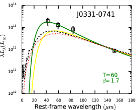
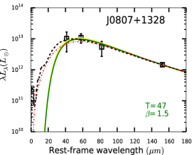
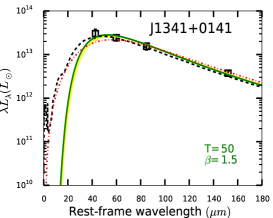
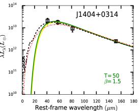
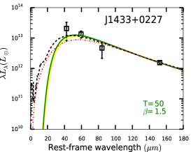
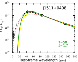
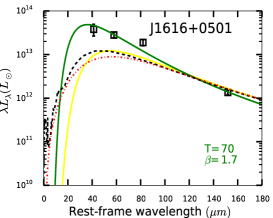
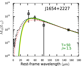
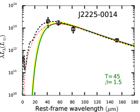
Figure 7: FIR SEDs for the nine FIR-bright quasars in our sample, including those already presented in T17. Data points correspond to Herschel/SPIRE measurements at 250, 350 and 500 $\mu$m and ALMA detections at 895 $\mu$m  (in the observed frame). For each source four model SEDs are presented: black-dashed lines represent the best-fitting FIR template from Chary & Elbaz (2001) while red-dotted lines represent the scaled SED from Magnelli et al. (2012). A scaled gray-body SED with $T_{\rm d}=47\,{\rm K}$ and $\beta=1.6$ is shown with a solid-yellow line, while a best fit model gray-body SED is shown with solid-green lines. The gray-body best fit parameters are included for each source.

We will rely on the rest frame FIR continuum emission to estimate the total FIR emission of our objects. This will allow us to determine the SFRs of the host galaxies and nearby SMGs using the well established relation between the FIR luminosity and the SFR (Kennicutt, 1989). We include in this analysis the objects already presented in T17.

For our FIR-faint objects this determination will be based only on the ALMA detection. For the FIR-bright objects, we will also use the Herschel measurements. We do not aim at performing a full modeling of the FIR Spectral Energy Distribution (SED), as the number of photometric points available do not allow for a determination of the several physical parameters necessary for that, but rather determine which set of SEDs better represent the observations.

The contribution to the FIR SED from the AGN should be small, commonly given as $\sim$10 $\%$ (e.g., Schweitzer et al. 2006; Mor & Netzer 2012; Rosario et al. 2012; Lutz et al. 2016). In this paper we assume that the FIR emission of the sources in our sample is dominated by dust heated by SF activity (see full discussion and many references in Netzer et al. 2016 and Lani et al. 2017). The alternative view which involves AGN heated dust contributing significantly to the FIR SED has been discussed in several publications (e.g., Duras et al., 2017; Leipski et al., 2014; Siebenmorgen et al., 2015; Schneider et al., 2015) but will not be addressed in this work. However, we do account for an additional error of the 250 $\mu$m Herschel/SPIRE band due to contribution from AGN-heated dust (as explained in N14, we add in quadrature an uncertainty estimated as 0.32 times the AGN luminosity at 1450Å). Taking this effect into consideration increases the error of the 250 micron measurement on average by a factor of 1.67. ALMA absolute flux calibration in band-7 is claimed to be of the order of 10%. We add this uncertainty in quadrature to the errors quoted in Table 2.

We use three different methods to produce model FIR SEDs for our sources. Because of the lower uncertainties in the ALMA measurements, this value usually dominates the fits for all three methods discussed.

For the first method we use the grid of FIR SEDs provided by Chary & Elbaz (2001, CE01). These templates are unique in shape and scaling. The best fit model is determined using the ALMA monochromatic luminosity and its associated uncertainty, while for the FIR-bright objects we also include the Herschel measurements (values and errors from N14, with the 250 $\mu$m flux error corrected as explained above). For FIR-faint objects the fit relies only on the ALMA measurement.

For the second method we scale the SED determined by Magnelli et al. (2012), which corresponds to an average from the most luminous SMGs in their work. As before, the Herschel measurements are included for those quasars with detections at 250, 350 and 500 $\mu$m.

For the third method we use a gray-body SED. Following T17 and other works, we use a temperature of $T_{d}=47$ K and dust emissivity coefficient $\beta=1.6$. However, since some of our sources are not well fitted using this set of parameters, we also try gray-body SEDs with a wider range of temperatures (40, 45, 50, 55, 60 and 70 K) and $\beta$ values (1.5 and 1.7). The determination of a best-fit temperature and $\beta$ is only possible for the FIR-bright, Herschel detected sources. The mean $\chi^{2}$ for our nine FIR-bright quasars is $\sim 2$ (for one degree of freedom). We show the SED fits in Figure 7 together with the best fit values, which are also reported in Table 4. We find that out of nine objects, seven are well fit by temperatures in the 40 to 50 K range.

Table 4: Galaxy Properties I

Sub-sample	Target		$\log L_{\rm CE}$	$\log L_{\rm Mag}$	$\log L_{\rm 47K\beta 1.6}$	$\log L_{\rm bestGB}$	$T_{\rm bestGB}$	$\beta_{\rm bestGB}$	SFRCE	SFRMag	SFR47Kβ1.6	SFRbestGB
	ID	Object	($L_{\odot}$)	($L_{\odot}$)	($L_{\odot}$)	($L_{\odot}$)	(K)		($M_{\odot}\,{\rm yr}^{-1}$)	($M_{\odot}\,{\rm yr}^{-1}$)	($M_{\odot}\,{\rm yr}^{-1}$)	($M_{\odot}\,{\rm yr}^{-1}$)
Bright	J0807	QSO	13.15	13.07	13.07	13.0	47	1.50	1405	1175	1170	1082
	J1404	QSO	13.40	13.31	13.29	13.3	50	1.50	2496	2033	1959	2135
	J1433	QSO	13.23	13.10	13.10	13.1	50	1.50	1688	1268	1262	1394
	J1616	QSO	13.23	13.11	13.13	13.7	70	1.70	1688	1289	1336	5275
	J1654	QSO	12.99	12.89	12.89	12.9	50	1.50	985	770	778	865
	J2225	QSO	13.44	13.34	13.32	13.3	45	1.50	2766	2201	2113	1796
	J0331	QSOT17	12.99	12.88	12.89	13.3	60	1.70	985	756	776	1922
	J1341	QSOT17	13.56	13.50	13.46	13.5	50	1.50	3613	3164	2911	3137
	J1511	QSOT17	13.40	13.26	13.26	13.4	50	1.70	2496	1838	1805	2262
	J1511	SMGT17	12.25	12.40	12.41	—	—	—	176	250	256	—
Faint	J1017	QSO	12.25	12.37	12.38	—	—	—	176	237	242	—
	J1151	QSO	11.93	12.12	12.13	—	—	—	86	131	134	—
	J1321	QSO	12.28	12.41	12.42	—	—	—	192	254	260	—
	J1447†	QSO	$<$11.06	$<$11.28	$<$11.29	—	—	—	$<$12	$<$19	$<$19	—
	J1447	SMG	12.68	12.79	12.80	—	—	—	482	620	634	—
	J2057	QSO	12.39	12.51	12.52	—	—	—	246	326	333	—
	J2057	SMG	11.83	11.99	12.00	—	—	—	67	98	100	—
	J2244	QSO	12.65	12.73	12.74	—	—	—	444	536	548	—
	J0923	QSOT17	12.56	12.68	12.69	—	—	—	362	477	487	—
	J0923	SMGT17	12.16	12.27	12.28	—	—	—	144	187	191	—
	J1328	QSOT17	12.32	12.43	12.44	—	—	—	207	270	276	—
	J1328	SMGT17	11.86	12.04	12.05	—	—	—	72	109	112	—
	J0935	QSOT17	12.28	12.41	12.42	—	—	—	192	255	261	—

Table 5: Galaxy Properties II

Subsample	Target		$\log M_{\rm dyn}^{uncorr}$	$\log M_{\rm dyn}$	$\log M_{Disp.}$	$\log M_{dust}$	$\log M_{BF}$	$\log M_{\rm BH}$	$M_{\rm dyn}/M_{\rm BH}$	$\dot{M}_{*}/\dot{M}_{\rm BH}$
	ID	Object	($M_{\odot}$)	($M_{\odot}$)	($M_{\odot}$)	($M_{\odot}$)	($M_{\odot}$)	($M_{\odot}$)	($M_{\odot}$)	($M_{\odot}$)
Bright	J0807	QSO	10.7	10.8	10.5	9.0	9.0	9.2	33	65
	J1404	QSO	10.9	11.4	10.7	9.2	9.2	9.5	81	130
	J1433	QSO	10.6	11.0	10.4	9.0	9.0	9.1	131	38
	J1616	QSO	10.9	11.1	10.7	8.9	8.7	9.4	49	71
	J1654	QSO	10.8	10.8	10.6	8.8	8.7	9.6	18	51
	J2225	QSO	10.7	11.0	10.5	9.2	9.2	9.3	53	82
	J0331	QSOT17	10.6	10.8	10.4	8.8	8.6	8.8	88	57
	J1341	QSOT17	10.7	10.9	10.5	9.4	9.4	9.8	11	111
	J1511	QSOT17	10.8	10.9	10.6	9.1	9.0	8.4	264	183
	J1511	SMGT17	10.8	10.8	10.6	…	…	…	…	…
Faint	J1017	QSO	10.0	11.0	9.8	8.3		8.7	178	32
	J1151$\sharp$	QSO	…	…	…	$<$8.0	…	8.8	…	27
	J1321	QSO	10.8	11.0	10.6	8.3	…	9.0	110	30
	J1447${\dagger}\sharp$	QSO	10.2	11.1	10.0	$<$7.2	…	8.0	1214	3
	J1447	SMG	10.0	10.2	9.8	8.7	…	…	..	…
	J2057	QSO	10.5	10.6	10.3	8.4	…	9.2	21	8
	J2057	SMG	11.0	11.0	10.8	7.9	…	…	..	…
	J2244	QSO	10.3	10.7	10.1	8.6	…	8.8	126	84
	J0923	QSOT17	10.5	10.9	10.4	8.6	…	8.7	158	60
	J0923	SMGT17	10.2	10.3	10.1	…	…	…	…	…
	J1328	QSOT17	10.1	10.8	9.8	8.3	…	9.1	50	24
	J1328	SMGT17	10.8	11.0	10.7	…	…	…	…	…
	J0935	QSOT17	10.4	10.6	10.3	8.3	…	8.8	56	20

Two require higher temperatures: J0331–0741 is best fit by a $\beta=1.7$ and $T_{d}=60$ K gray-body SED while J1616+0501 needs $\beta=1.7$ and $T_{d}=70$ K. We briefly discuss these two cases next.

For J1616 all the Herschel photometric points are found more than 3$\sigma$ above the CE01 best-fit template, which is dominated by the scaling to the ALMA measurement. The corresponding SFR from the gray-body best fit is 5275 $M_{\odot}\,{\rm yr}^{-1}$  even higher than the $\sim 4200$ $M_{\odot}\,{\rm yr}^{-1}$ found by N14 based on Herschel data only. A similar, although not as extreme case is J0331, whose data were already presented in T17. For J0331 N14 determined a SFR of $\sim 2100$ $M_{\odot}\,{\rm yr}^{-1}$, in good agreement with the value of 1922 $M_{\odot}\,{\rm yr}^{-1}$ we determine from the gray-body best fit. Clearly, the high SFRs determined for these sources are driven by their very high Herschel luminosities. The high gray-body temperatures, on the other hand, are the result of the correspondingly steep SEDs, which are found once the ALMA data are also taken into account.

Gray-body temperatures as high as $T_{d}=60-70$ are not expected for star-forming sources. However, temperatures as high as 70 or 80 K have been recently determined for a very small fraction of SMGs at high-redshift (Miettinen et al., 2017), so these rather high ISM temperatures might not be totally unusual in the most luminous sources, although more observations are necessary in order to confirm this.

Once the total IR luminosity is determined by integrating the SED over the 8-1000 $\mu$m range, the SFR is obtained using $\rm SFR/M_{\odot}\,{\rm yr}^{-1}=L_{\rm FIR}\ /10^{10}L_{\odot}$, which assumes a Chabrier Initial Mass Function (IMF). The results are presented in Table 4 as $L_{\rm CE}$ and SFR_CE for the CE01 fits, $L_{\rm Mag}$ and SFR_Mag for the Magnelli et al. (2012) fits, $L_{\rm 47K\beta 1.6}$ and SFR_47Kβ1.6 for the gray-body fit with fixed parameters $T_{d}=47$ K and $\beta=1.6$, and as $L_{\rm bestGB}$ and SFR_bestGB for the gray-body fit with $T_{d}$ and $\beta$ left as free parameters.

For our total sample of 18 quasars, we see that the FIR-bright targets have a SFR range of $\sim 900-3200$ $M_{\odot}\,{\rm yr}^{-1}$, the FIR-faint objects have a range of $\sim 200-500$ $M_{\odot}\,{\rm yr}^{-1}$, and the SFRs of the SMGs cover $\sim 90-600$ $M_{\odot}\,{\rm yr}^{-1}$. The difference in the determined SFRs using the different methods illustrates the systematic uncertainties of these calculations.

Besides the FIR-bright sources presented in Figure 7, Table 4 also lists the SFRs obtained for the FIR-faint sources. The SED best-fit values for J1447 are based on the ALMA continuum upper limit previously determined. We found this object to have an extremely low SFR of $<20$ $M_{\odot}\,{\rm yr}^{-1}$, maybe indicating that effective starformation quenching has already occurred. The detection of [C ii] in this host showcases how this line can be detected in the ISM of galaxies with very little on-going star formation. In the following sections we will take the average SFR obtained from these methods as the representative SFR for each object. Errors will be computed as the maximum and minimum derived SFR.

3.1.3 The $L_{\rm AGN}$ versus $L_{\rm SF}$ plane

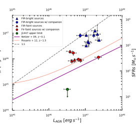
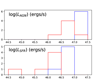
Figure 8: Top: $L_{\rm SF}$ versus $L_{\rm AGN}$ for our FIR-bright (blue markers) and FIR-faint sources (red markers), as well as the upper limit of J1447 (green marker) with an arrow to indicate it is an upper limit. Those sources with companions are marked as a circle. The orange curve for redshift $0.8-1.5$ from Rosario et al. (2012) and scaled up by a factor of two to allow for the difference between L(60 $\mu$m) used in that paper and the $L_{\rm SF}$ used in our work. The correlation for AGN dominated sources is shown as a solid purple and is taken from Netzer (2009) as $L_{\rm SF}\simeq 10^{43}(L_{\rm AGN}/(10^{43}{\rm erg\,s}^{-1}))^{0.7}$. The dashed straight line corresponds $L_{\rm AGN}$ = $L_{\rm SF}$, shown for reference. Bottom: Logarithmic distributions of $L_{\rm SF}$ and $L_{\rm AGN}$ in units of ergs s^-1.

Figure 8 presents the $L_{\rm AGN}$ versus $L_{\rm SF}$ plane. FIR-bright and FIR-faint objects are shown with different colors, while the presence of companions is shown using different symbols.

Since our luminosity ranges in $L_{\rm AGN}$ and $L_{\rm SF}$ are rather narrow, it is not possible to draw conclusions about how our sources compare with those trends found by previous works for $L_{\rm AGN}$ and $L_{\rm SF}$-dominated sources. In fact, it has been a matter of great debate why the $L_{\rm AGN}$ versus $L_{\rm SF}$ plane shows significantly different trends depending on the way samples are defined (e.g., see discussion in Netzer et al. 2016). The answer to the apparent contradictory results seems to reside in the stochastic nature of AGN activity, with duty cycles much shorter than those that characterize star formation (e.g., Hickox et al., 2014; Volonteri et al., 2015; Stanley et al., 2015). In short, selecting samples based on SFR and binning them in AGN power, will give a representative $L_{\rm AGN}$-$L_{\rm SF}$ relation since the rapid ($\sim 10^{5-6}$ yr) changes in AGN power will be smoothed out, while selecting them in $L_{\rm AGN}$ and binning in $L_{\rm SF}$ will mix-and-match objects selected from their ‘unrepresentative’ AGN luminosity and with very different SF power. These observed differences, however, seem to saturate at the highest luminosities.

In Figure 8 we include a 1:1 $L_{\rm AGN}$-$L_{\rm SF}$ line as well as the trends determined by Netzer (2009) from observations at a wide redshift range and Rosario et al. (2012) at $z\lesssim 2$, both of which defined for bright AGN but dominated by local samples in the case of Netzer (2009) and from samples drawn from deep field surveys in the case of Rosario et al. (2012), hence not including the most powerful AGN. It is therefore not surprising that our optically flux-limited selected sample of quasars on average, sits above both the Netzer (2009) and Rosario et al. (2012) relations. This is particularly true for the bright-FIR subsample. It would be of great interest to compare the $L_{\rm AGN}$ and $L_{\rm SF}$ distributions of our sources with those of higher redshift, like that of Decarli et al. (2018). However, quasars found at $z>5$ are very hard to find because of a strong contamination of late brown dwarfs, which introduces severe and complex selection biases to those systems (Banados et al., 2016).

Inspection of Figure 8 shows that the our FIR-bright and FIR-faint populations occupy distinctively different regions of the diagram, even though the individual distributions of these two properties do not show evidence for two separated populations, as can be seen in the bottom panel of Figure 8. This can also be seen in Figure 2 of Netzer et al. (2014) (as $\lambda L_{\lambda}$(3000Å)) who analyzed the Herschel observations of $z\sim 4.8$ quasars, including all our FIR-bright and FIR-faint sources, and 20 further FIR-faint sources. From this work it becomes clear that FIR-bright and FIR-faint sources dominate at the high and low-end of the BH mass distribution, respectively, but with no indication of a bimodality. In fact, the distributions of the source properties indicate a clear relation between BH mass, $L_{\rm AGN}$, and SFRs with the median $M_{\rm BH}$, $L_{\rm AGN}$, and $L_{\rm SF}$ of the FIR-bright sources (9.28 $M_{\odot}$, $10^{47.13}$ erg s^-1, and $10^{46.91}$ erg s^-1, respectively) being higher than those of the FIR-faint sources(8.85 $M_{\odot}$, $10^{46.78}$ erg s^-1, $10^{46.23}$ erg s^-1). For a more in depth discussion see Netzer et al. (2014).

We find a weak correlation coefficient between $L_{\rm AGN}$ and $L_{\rm SF}$ for our entire sample ($r=0.55$), however more extensive studies (e.g., Stanley et al. 2015, 2017; Lanzuisi et al. 2017) indicate that much larger samples are required to draw conclusions. We will return to the issue of the possible segregation observed in the $L_{\rm AGN}$ versus $L_{\rm SF}$ plane in Section 3.1.6.

3.1.4 Dust masses

The continuum emission at rest wavelength $\sim$ 152 $\mu$m can also be used to calculate dust masses for our objects assuming that the FIR continuum flux originates from optically thin dust at these wavelengths. Using the same methods as in Dunne et al. (2000) and Beelen et al. (2006) (see also, Scoville et al. 2016), the dust mass can be calculated as:

$$M_{d}=\frac{S_{\lambda rest}D_{L}^{2}}{\kappa_{d}(\lambda_{rest})B(\lambda_{rest},T_{d})}$$ (1)

where $\kappa_{d}(\lambda)\propto\lambda^{-\beta}$ is the wavelength dependent dust mass opacity, $S_{\lambda rest}$ is the continuum flux density at $\lambda rest$, $B(\lambda_{rest},T_{d})$ is the monochromatic value of the Planck function at $\lambda_{rest}$ for temperature $T_{d}$, and $D_{L}$ is the luminosity distance. $\kappa_{d}$ is found to be 0.077 m² kg^-1 at 850 $\mu$m (Dunne et al., 2000), and hence, $\kappa_{d}(\lambda_{rest})=0.077\ (850/\lambda_{rest})^{\beta}$ m² kg^-1. To calculate the dust mass we assume $T_{d}=47\,$ K and $\beta=1.6$.

We note from equation (1) that the only formal error comes from the measurement of the continuum flux, while systematic errors will arise from our assumption of the adopted SED and the opacity coefficient, which will dominate. However, as we are using very similar parameters to those adopted in the literature a direct comparison of results is possible.

We derive dust masses for our full sample of 16 continuum detected quasars and find a range of $M_{dust}\sim 2-15\times 10^{8}M_{\odot}$ (see Table 5). Upper limits of $\sim 10^{8}M_{\odot}$ and $\sim 10^{7}M_{\odot}$ are found for J1151 and J1447 hosts, respectively. The average value is larger for FIR-bright objects than for FIR-faint objects, with dust masses of $10^{9.0}$ and $10^{8.4}M_{\odot}$, respectively. In Table 4 we also determine dust masses for the FIR-bright objects using the best fit values of $T_{bestGB}$ and $\beta_{bestGB}$ discussed in Section 3.1.2. However, we note that due to the small range of $T$ and $\beta$ and the dominance of the continuum flux density and luminosity distance, the differences in these calculations from assuming $T_{d}=47\,$ K and $\beta=1.6$ are minor.

We derive dust masses for our full sample of 16 continuum detected quasars and find a range of $M_{dust}\sim 2-15\times 10^{8}M_{\odot}$ (see Table 4). Upper limits of $\sim 10^{8}M_{\odot}$ and $\sim 10^{7}M_{\odot}$ are found for J1151 and J1447 hosts, respectively. The average value is larger for FIR-bright objects than for FIR-faint objects, with dust masses of $10^{9.0}$ and $10^{8.4}M_{\odot}$, respectively. In Table 4 we also determine dust masses for the FIR-bright objects using the best fit values of $T_{bestGB}$ and $\beta_{bestGB}$ discussed in Section 3.1.2. However, we note that due to the small range of $T$ and $\beta$ and the dominance of the continuum flux density and luminosity distance, the differences in these calculations from assuming $T_{d}=47\,$ K and $\beta=1.6$ are minor.

3.1.5 Companion detections

Current cosmological models recognize high-z quasars as sign-posts of high-density environments (see Costa et al. 2014 and references therein). It is therefore not unexpected that our sample shows a larger number of companions when compared to ALMA observations of blank fields.

Recent blank deep field surveys conducted with ALMA (Carniani et al., 2015; Aravena et al., 2016a; Fujimoto et al., 2016) imply that each ALMA pointing of 18^′′ should have of the order of $\sim$ 0.1 SMGs at a flux limit of 15 $\mu$Jy at 1.2mm. Other measurements of the HST Legacy Fields (Bouwens et al., 2015) and the Great Observatories Origins Deep Survey (GOODS) Fields (Stark et al., 2009) give surface densities on the order of 0.01 galaxies per single ALMA band-7 pointing (for SMGS with SFR $\sim 100\,M_{\odot}\,{\rm yr}^{-1}$). Though they have not been confirmed with higher S/N, Aravena et al. (2016b) cites a number count of roughly 0.06 [C ii]-emitting $z\sim 5-8$ galaxies per ALMA pointing of the Hubble Ultra Deep Field.

As quasars, SMGs are also highly clustered and seem to be hosted by massive dark matter halos (Wilkinson et al., 2017). Besides, several works have found that a substantial fraction of sub-mm sources with multiple components, varying from 35 to 80 percent, depending on resolution and flux limit (Hodge et al., 2013; Bussmann et al., 2015; Scudder et al., 2016; Hayward et al., 2018).

In a recent study of multiplicity of far-infrared bright quasars, Hatziminaoglou et al. (2018) assembled a random sample of 28 infrared-bright SDSS quasars with detections in Herschel/SPIRE. This sample of detected quasars would correspond to our FIR-bright objects in terms of $L_{AGN}$, $M_{BH}$, and Eddington ratios, but with $z\sim 2-4$. Using the ALMA Atacama Compact Array (ACA) Hatziminaoglou et al. (2018) found that 30 percent of their targets were found to be multiple. However, their observations do not provide the same depth or resolution as our own, and the redshifts of their sub-mm sources were not confirmed.

Decarli et al. (2017, 2018) present a similar study of [C ii] and dust continuum at a similar redshift to our study, where the ALMA observations provide enough information to indicate whether the nearby sources are real companions. They found that 4/25 rapidly star-forming galaxies have a companion, i.e., 16 percent. Based on the IR-luminosities reported by Decarli et al. (2018), 20 quasars hosts would be classified as FIR-faint for a threshold FIR luminosity of $10^{12.9}$ $L_{\odot}$, and 3/4 of the companions would be associated to FIR-faint quasar hosts.

With the two newly observed companions we present here, our total observed sample of 18 quasars has 5 sources with companions, 1 FIR-bright (J1511) and 4 FIR-faint (J0923, J1328, J2057, and J1447), i.e., 28 percent. J0923 and J1328 have no nearby sources in Spitzer/IRAC, while J2057 and J1447 were not observed by Spitzer. J1511 (T17) has two further nearby Spitzer/IRAC sources. It is interesting that we only find that 1 FIR-bright target is multiple in ALMA observations, a rate much lower than that found in the randomly selected FIR-bright sample of Hatziminaoglou et al. (2018), and that we find a percentage of companions slightly higher than that reported by Decarli et al. (2017).

3.1.6 Major mergers among hosts

Different lines of evidence suggest that mergers among gas-rich galaxies should drive the most luminous AGN and the most powerful starformation of their hosts. This is proposed by numerical simulations (Hopkins et al., 2005, 2008) and also backed by observations at low and high-$z$ (Treister et al., 2012; Glikman et al., 2015; Koss et al., 2018). Thus our initial expectations were to find that our ALMA observations would show that the FIR-bright sources are powered by major mergers of gas-rich galaxies, and that the FIR-faint sources, found closer to the main sequence of galaxies, could be evolving through a secular process or also involved in mergers. The evidence would emerge from the presence of close companions to our quasars.

We find that of the $\sim 28$ % host galaxies with companions the majority are FIR-faint sources (1 FIR-bright and 4 FIR-faint). One FIR-bright source, J1404, presents an unusual [C ii] double peak that could signal a late stage merger. Bischetti et al. (2018) found three companions around their targeted $z=4.4$ quasar, two of which have double-peaked line emission, while in Willott et al. (2017), the high spectral and spatial resolution allows them to attribute different peaks in the [C ii] line to the quasar source, a 5 kpc separated companion, and a ”central excess” component between the two.

The lack of companions to FIR-bright quasars is in fact problematic, as it is usually assumed major mergers between gas-rich galaxies to be the triggering mechanism for starbursting galaxies. Note, however, that recent ALMA observations at $z\sim 4.5$, suggest that minor-mergers might also locate systems above the main sequence (Gómez-Guijarro et al., 2018).

The preference for companions in FIR-faint sources could then be explained if these correspond to very early stages in the merger process, while the FIR-bright systems correspond to much later stages, when the progenitor galaxies are no longer resolved by our ALMA observations. The lack of disturbances in the velocity fields of our systems does not oppose this argument, as observations of the ISM in low-$z$ mergers demonstrate that the central core of mergers rapidly settles into a rotating-dominated system (Ueda et al., 2014).

The lack of clear, ‘on-going’ mergers among our systems could be explained as a sample bias since our quasars were optically selected. Glikman et al. (2015) has shown that for a sample of 2MASS selected dust-reddened quasars at $z\sim 2$, 8/10 hosts show clear evidence for very close, interacting companions. Similar results were found by Urrutia et al. (2008) for dust-reddened quasars at $z\sim 0.4-1.0$. The nuclei are so heavily dust-enshrouded that HST follow up clearly revealed the perturbed hosts. These type of quasars would not be found in our parent sample. It is then possible that the distinct populations observed in the $L_{\rm AGN}$-$L_{\rm SF}$ plane (Figure 8) reflect the properties of the very early and very late mergers just mentioned.

3.2 Other Determinations

3.2.1 Dynamical Masses

The $\left[{\rm C}\,\textsc{ii}\right]$ line can be used to estimate the dynamical masses ($M_{\rm dyn}$) of the quasar host galaxies and the companion SMGs. We use the same method as in T17 and several other studies of [C ii] and CO emission in high-redshift sources, which assumes the [C ii]-traced ISM is arranged in an inclined, rotating disk (Wang et al., 2013; Willott et al., 2015; Venemans et al., 2016), and determine $M_{\rm dyn}$ as:

$$M_{\rm dyn}=9.8\times 10^{8}\left(\frac{D_{\left[{\rm C}\,\textsc{ii}\right]}}{{\rm kpc}}\right)\left[\frac{{\rm FWHM}\left[{\rm C}\,\textsc{ii}\right]}{100\,\,{\rm km\,s}^{-1}}\right]^{2}\,\frac{1}{\sin^{2}\left(i\right)}\,\,M_{\odot}\,\,.$$ (2)

In this relation $D_{\left[{\rm C}\,\textsc{ii}\right]}$ is the size of the [C ii]-emitting region measured by the deconvolved major axis of the Gaussian fit of said region (see Table 2). The $\sin\left(i\right)$ term reflects the inclination angle between the line of sight and the polar axis of the host gas disks, with the circular velocity given as $v_{\rm circ}=0.75\times{\rm FWHM}/\sin\left(i\right)$. i is determined from the ratio $\cos\left(i\right)=\left(a_{\rm min}/a_{\rm maj}\right)$, where $a_{\rm min}$ and $a_{\rm maj}$ are the semi-minor and semi-major axes of the [C ii] emitting regions, respectively. These masses can be found in Table 5, where we list $M_{\rm dyn}$ as well as its inclination uncorrected value (i.e., $M_{\rm dyn}^{uncorr}=M_{\rm dyn}\times\sin^{2}(i)$). We also include the values determined in T17.

We find that the FIR-bright and FIR-faint systems have comparable $M_{dyn}$ values. The mean is $9\times 10^{10}$ $M_{\odot}$. We also note that among the interacting SMGs reported in this work the companion to J1447 is of particular interest. Its two [C ii] spectral components taken individually, each with unresolved sizes, would correspond to systems with comparable dynamical masses found at the lower end of the observed range presented in Table 5. Therefore they would represent a major merger between these two components, but a likely minor merger with the quasar host. Note, however, that the dynamical mass of the J1447 host is also particularly uncertain, due to the weakness of the [C ii] detection.

This method of deriving the dynamical mass carries significant uncertainties, due to the several assumptions required to derive them, and to the limited spatial resolution data available for our systems. A large contributor to the error is our measurement of the major and minor axis of the [C ii] emitting region, from which we derive $i$ and $D_{\left[{\rm C}\,\textsc{ii}\right]}$. We estimate a mean error of 0.44 dex by propagating systematic uncertainties and the uncertainties of our measured values.

However, the most significant assumption is that we are observing inclined rotating disks. Only 4/6 of our FIR-bright and possibly 2/4 of our FIR-faint objects show clear indications of a smooth and coherent velocity gradient, as can be seen in Figure 4. Furthermore, note that even a smooth and coherent velocity gradient does not guarantee a rotation dominated host galaxy. We can compute the dynamical masses assuming the case of pure dispersion-dominated gas (Decarli et al., 2018):

$$M_{\rm Disp}=\frac{3}{2}\frac{a_{\rm maj}\sigma_{line}^{2}}{G}$$ (3)

where $\sigma_{line}$ is the line width of the Gaussian fit of the [C ii] spectrum, G is the gravitational constant, and $a_{\rm maj}$ again is the major axis of the [C ii]-region. We find that the dynamical masses we derive from assuming dispersion-dominated gas is lower than both the inclination corrected and non-corrected dynamical masses derived from assuming a rotating disk, with a mean of $2.4\times 10^{10}$ $M_{\odot}$ for $M_{\rm Disp}$ (see Table 4). Dynamical masses derived from assuming dispersion-dominated gas can be regarded as a lower limit to the true dynamical mass. We will use the dynamical masses obtained assuming an inclined, rotating disk throughout this rest of the work in order to be comparable to similar studies in the literature.

3.2.2 Gas Masses

We can determine gas masses, $M_{gas}$, making use of a gas-to-dust ratio (GDR) of 100, as determined at low-$z$ (Draine et al., 2007). Recent studies comparing gas mass estimates obtained from CO line measurements and dust masses obtained from FIR emission have given a wide range of GDRs for high-redshift systems ($\sim 30-100$) (Ivison et al., 2010; Aravena et al., 2016c; Banerji et al., 2017). This is an unexpected result, since it is well established that high-$z$ galaxies are characterized by lower metallicities at all galaxy masses (Lian et al., 2018) and that the GDR is inversely proportional with metallicity (Rémy-Ruyer et al., 2014; De Vis et al., 2019). However, as discussed in Aravena et al. (2016c) and Banerji et al. (2017), another interpretation for these results is to assume a ‘normal’ GDR and revisit the determination of the CO luminosity to total gas conversion factor. Both, the GDR and CO luminosity to total gas fraction are highly dependent on galaxy properties, such as surface density, compactness, and particularly, metallicity. In summary, and for a more straight forward comparison with other works, we adopt a GDR of 100.

Gas masses are derived from dust masses in Table 5 and are found to be large, in the $10^{10-11}M_{\odot}$ range. For four of our FIR-bright systems $M_{gas}$ are larger than the dynamical masses by factors of up to three, while for only one FIR-faint system $M_{gas}\sim 0.9\times M_{\rm dyn}$, the remaining showing factors ranging from 0.7 to 0.2.

In general the estimated ISM masses for our quasars are comparable to their dynamical masses. For our FIR-bright sources, 6/9 show $M_{gas}\geq M_{dyn}$, by factors 1-3 (the unphysical finding that $M_{gas}>M_{dyn}$ would be alleviated had we adopted a GDR as low as 30, as discussed above). This is not seen for the FIR-faint sources, suggesting that FIR-bright objects are more gas rich than FIR-faint systems. Defining $f_{gas}\equiv M_{gas}/M_{dyn}$, we find for those objects where $M_{gas}<M_{dyn}$ that $f_{gas}=0.2-1.0$.

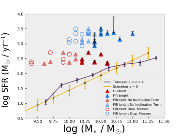
Figure 9: Stellar mass versus Star Formation Rate – the main sequence of starforming galaxies – for our quasars. Bright and faint FIR sources are shown with different colors. Only seven FIR-faint objects are plotted as J1447 is not detected significantly in continuum or [C ii], while J1151 is a complete non-detection. The dynamical mass and SFR values are taken from Table 4. We assume $M_{\star}=0.4\ M_{\rm dyn}$, as explained in Section 3.2.3. We include the MS curves given in Equation (9) of Schreiber et al. (2015) (shown in yellow) and that of Tomczak et al. (2016) (in purple). The opaque red and blue triangles are our inclination corrected dynamical masses, while the transparent triangles are the inclination uncorrected dynamical masses. The dynamical masses calculated assuming dispersion dominated gas are plotted as circles.

3.2.3 The Main Sequence at $z\sim 5$

We want to compare our full quasar sample with galaxies found on the stellar mass – SFR sequence for starforming systems, the ‘main sequence’ (MS), at similar redshifts. However, we only have estimates for the total dynamical and gas masses of our quasar hosts, not of their stellar masses. In principle, these could be obtained calculating $M_{\star}=M_{\rm dyn}-M_{gas}$. From the measured values there is a strong indication that most of the quasars hosts are very gas rich, with $M_{gas}=0.3-4.0\ M_{\star}$, for those objects where $M_{gas}<M_{dyn}$, and possibly higher for those objects where $M_{gas}>M_{dyn}$. As already explained, the uncertainties on these values are significant.

An alternative approach is to adopt a gas fraction measured in non-active high-$z$ galaxies where the stellar mass can be determined directly, which is not possible for our sample because of the dominance of the AGN continuum at rest-frame near-IR and optical bands. These determinations have been done out to $z\sim 4$ (Schinnerer et al., 2016; Dessauges-Zavadsky et al., 2017; Darvish et al., 2018; Gowardhan et al., 2019), and found $f_{gas}\sim 0.5-0.8$ (considering no dark matter), where a strong dependence with redshift and no correlation with environment are also seen (Darvish et al., 2018). We can then conservatively assume that for our systems $f_{gas}=M_{gas}/M_{dyn}=0.6$ and therefore $M_{\star}=0.4\ M_{\rm dyn}$.

In Figure 9, we plot two MS curves. One is the parameterization given in Equation (9) of Schreiber et al. (2015) for redshift ranges $4<z<5$, after correcting for the different adopted IMF (Schreiber et al. 2015 uses a conversion factor of SFR to $L_{SF}$ 1.7 times larger than our own). The second curve is from Tomczak et al. (2016), for galaxies at redshifts $0.5<z<4$. Both MS curves agree well with each other.

We find that the majority of our sources lie above the MS curves. If we used dynamical mass values derived from assuming dispersion-dominated gas, our objects would shift to the lower stellar mass regime and sit even higher above the MS, as seen in Figure 9. Clearly, all of our FIR-bright quasars are found in the starbursting domain and at least 1 dex from the MS. Their SFRs are only comparable to the brightest known SMGs. Some of the FIR-faint sources sit within 1$\sigma$ of the MS of starforming galaxies at those early epochs, but again, the majority of our faint sources sit above the MS. Note that our division into FIR-bright and FIR-faint sources is completely arbitrary, and the determined SFRs for our full sample is indeed a continuous distribution, as shown in the bottom panel of Figure 8.

3.2.4 SMBH–Host Galaxy Mass Relation

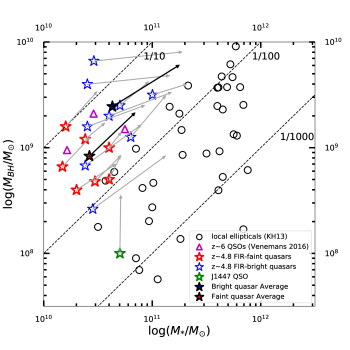
Figure 10: Black hole masses, $M_{\rm BH}$, vs. host galaxy stellar masses, $M_{\star}$, for our sample of $z\sim 4.8$ quasars. FIR-bright objects are marked with blue stars, FIR-faint objects are marked with red. For comparison we also plot a sample of $z\simeq 0$ elliptical galaxies taken from Kormendy & Ho (2013) shown as black circles. The dotted diagonal lines trace different constant BH-to-host mass ratios. Grey arrows indicate the possible evolution in both the BH and stellar components, assuming constant mass growth rates over a period of 50 Myr. Filled stars with black arrows indicate average values and growth for both FIR-faint and bright objects. Our plotted sources have a typical error of 0.44 dex for $M_{\star}$ (from our own estimates) and 0.4 dex for $M_{\rm BH}$ (derived in T11).

In Figure 10, we plot the stellar masses of our quasar hosts against their black hole masses for the full sample of nine FIR-bright and eight FIR-faint quasars detected in [C ii]. As before, we have adopted $M_{\star}=0.4\ M_{\rm dyn}$. However, it is likely that the real values of $M_{\star}$ would broaden the observed distribution, which now corresponds to a net shift of the observed $M_{\rm dyn}$ distribution. Black Hole masses were taken from T11 and are based on Mg ii measurements. We find that the average black hole mass of our sample is $10^{9.2}$$M_{\odot}$, with a slight difference between the black hole properties of FIR-bright and -faint objects. FIR-bright objects having an average $M_{\rm BH}$ of $10^{9.4}M_{\odot}$ and Eddington ratio of $L/L_{\rm Edd}\sim 0.65$, while FIR-faint objects have an average $M_{\rm BH}$ and Eddington ratio of $10^{8.9}M_{\odot}$ and 0.78 respectively. We find a mean $M_{BH}/M_{\star}$ ratio of 1/19, with FIR-bright sources having $M_{BH}/M_{\star}=1/15$ and FIR-faint systems 1/28.

We compare our sample with the local massive elliptical galaxies (Kormendy & Ho, 2013) , Figure 10 shows the positions of local galaxies with a $M_{BH}/M_{\star}$ ratio ranging from $\sim 1/100$ to $\sim 1/1000$, the ratios being strongly correlated with mass. While the black hole masses of our sample of high-$z$ luminous quasars are found at similar values as seen in the local universe, the stellar masses are on average one order of magnitude lower. This is similar to the results found by other groups and is in good agreement with the direct detection of two quasars hosts at $z\sim 4$ (Targett et al., 2012). A higher redshfit sample of three quasars at redshift $z\sim 6.8$ with available $M_{\rm BH}$, $M_{*}$, $L/L_{\rm Edd}$, and SFRs is found in Venemans et al. (2016). $M_{\rm BH}$ values were taken from De Rosa et al. (2014). When compared to our own sample in Figure 10 we see that they sit between the FIR-bright and FIR-faint objects with an average $M_{BH}/M_{\star}$ ratio of 1/19, the same as our sample. In terms of their AGN properties they are found at the top end of the mass distribution of $z\simeq 6$ sources presented in T11, but at the low end in terms of $L/L_{\rm Edd}$. Their SFRs are somewhat in between our FIR-bright and FIR-faint objects. We include these 3 sources in our Figure 10. As we already pointed out, it is not possible to derive any conclusions from a direct comparison between sources at $z\sim 5$ and $z\sim 6$ because of the very different way these samples have been defined.

Assuming that the stellar mass of the quasar host galaxies grows only due to the formation of new stars (i.e., neglecting possible mergers), we can use our SFR estimates from Section 3.1.2 to calculate the growth rate of $M_{\star}$, i.e., $\dot{M}_{\star}$. The instantaneous growth rate of the black holes can be computed as the mass accreted onto the black hole which does not convert into energy: $\dot{M}_{BH}=\frac{1-\eta}{\eta}\frac{L_{bol}}{c^{2}}$, where $L_{bol}$ is the bolometric luminosity from T11 using the rest-frame UV continuum emission. We assume the radiative efficiency to be $\eta=0.1$.

As in T17 we find that all systems have $\dot{M}_{BH}/\dot{M}_{\star}>1/200$ and typical values are found to be $\sim 1/54$ (see Table 4), with the FIR-bright and FIR-faint systems having medians of $\dot{M}_{BH}/\dot{M}_{\star}\simeq 1/71$ and $1/27$ respectively.

Assuming that the calculated instantaneous growth rates continue for a period of time, we can determine the migration that our sources would undergo on the $M_{BH}$ vs $M_{\star}$ plot. The time span needs to be determined under reasonable assumptions. Typical starformation time scales derived at lower redshifts might not be applicable to our sample. Using the determined $M_{g}$ and SFRs we can find the depletion time for the observed reservoir of gas. This is found to be between 20 to 100 Myr. Hence, we will adopt a general time span of 50 Myr, which is also what was used in T17.

As already discussed, because of the stochastic nature of AGN activity, with duty cycles shorter than those of star-formation by one or perhaps up to two orders of magnitude (e.g., Hickox et al., 2014; Volonteri et al., 2015; Stanley et al., 2015), the instantaneous $\dot{M}_{BH}$ values measured for single objects might not be the best proxy to characterize black hole growth over the time required for the build up a sizable stellar mass due to star formation. Instead, the value averaged over our entire sample will result in better determination of the ‘typical’ $\dot{M}_{BH}$. The resulting ‘growth tracks’ are shown in Figure 10. We also obtained the means of $\dot{M}_{BH}$ and $\dot{M}_{\star}$ separately for the FIR-bright and FIR-faint subsamples and have plotted them in Figure 10. For most objects these tracks suggest a larger future growth of stellar mass over BH mass, which is necessary to bring them closer to the local population of elliptical galaxies.

4 Summary and Conclusion

We have presented new band-7 ALMA observations for twelve new luminous quasars at $z\simeq 4.8$, to reach a total sample size of 18 sources, which are divided into Herschel/SPIRE detected (FIR-bright) and Herschel/SPIRE undetected (FIR-faint) systems. The data probes the rest-frame far-IR continuum emission that arises from dust heated by SF in the host galaxies of the quasars, and the [C ii] $\lambda 157.74\,\mu{\rm m}$ emission line from the host ISM. The ALMA observations resolve the continuum- and line-emitting regions on scales of $\sim 2$ kpc.

Our main findings for our total sample of 18 targets is as follow.

1. 5/18 of our quasars have companions, four of the quasars are FIR-faint and one is FIR-bright. The companions are separated by 15 - 60 kpc. The quasar hosts with companions have a SFR rate of $\sim$ 220 - 3200 $M_{\odot}\,{\rm yr}^{-1}$. The companions are forming $90-580\,M_{\odot}\,{\rm yr}^{-1}$ which is generally lower than the SFR measured for the quasar hosts.

2. The dynamical masses of the quasar hosts, estimated from the [C ii] lines, are within a factor of $\sim 3$ of the masses of the interacting companions, supporting an interpretation of these interactions as major mergers.

3. For all our sources, we find that the gas mass is comparable to the dynamical mass, suggesting that some of them could be kinematically dominated by the ISM component.

4. The [C ii]-based dynamical masses show that our systems are above the “main sequence” of star-forming galaxies. When comparing $L_{\rm AGN}$ vs $L_{\rm SF}$ we find evidence that the FIR-bright and FIR-faint subsamples are separated. We tentatively interpret this result as an evolutionary sequence within merger evolution, but great caution must be exercised as this is based on small number statistics.

5. Compared with the BH masses, the [C ii]-based dynamical host masses are generally lower than what is expected from the locally observed BH-to-host mass ratio.

6. We have found a clear blueshift of Mg ii with respect to our [C ii] measurements which is not observed at lower redshifts. No correlation is found between the shift and the presence of companions or the accretion rate of the supermassive black holes.

7. The lack of companions to most of our quasar hosts may suggest that processes other or besides major mergers are driving the significant SF activity and fast SMBH growth in these systems. Alternatively, the systems could be observed at very different stages of the merger process, with most FIR-faint sources found at the early stages, while FIR-bright are found at very late phases.

Table 6: Compiled Offset List

Source	Target	$\left[{\rm C}\,\textsc{ii}\right]\ -{\rm Mg}\,\textsc{ii}\$	$L/L_{\rm Edd}$	log $L_{\rm IR}$	Mg ii Paper
		km s-1
Trakhtenbrot et al. 2017	SDSS J033119.67–074143.1	$+$412	1.202	13.05	Trakhtenbrot et al. 2011
	SDSS J134134.20+014157.7	$+$573	0.1819	13.51	…
	SDSS J151155.98+040803.0	$+$456	1.1819	13.31	…
	SDSS J092303.53+024739.5	$-$213	0.6606	12.65	…
	SDSS J132853.66-022441.6	$-$621	0.3548	12.40	…
	SDSS J093508.49+080114.5	$+$588	0.741	12.37	…
This Work	SDSS J080715.11$+$132805.1	$+$256	0.447	13.08	…
	SDSS J140404.63$+$031403.9	$+$2208	0.219	13.33	…
	SDSS J143352.21$+$022713.9	$+$379	1.230	13.15	…
	SDSS J161622.10$+$050127.7	$+$620	0.537	13.38	…
	SDSS J165436.85$+$222733.7	$-$112	0.199	12.93	…
	SDSS J222509.19$-$001406.9	$+$340	0.617	13.35	…
	SDSS J205724.14$-$003018.7	$+$1064	0.891	12.48	…
	SDSS J132110.81$+$003821.7	$+$337	0.355	12.37	…
	SDSS J224453.06$+$134631.6	$+$225	0.676	12.71	…
	SDSS J101759.63$+$032739.9	$+$1605	0.549	12.34	…
	SDSS J144734.09$+$102513.1	$-$224	1.995	11.23	…
Decarli et al. 2018	SDSS J084229.43$+$121850.4	$+$310	0.7	12.20	De Rosa et al. 2011
	SDSS J130608.26+035626.3	$+$757	0.792	12.50	Kurk et al. 2007
	CFHQS J1509-1749	$+$63	0.68	12.59	Willott et al. 2010
	CFHQS J2100-1715	$-$245	0.49	11.77	…
	PSO J231.6576–20.8335	$-$340	0.48	13.04	Mazzucchelli et al. 2017
	VIKING J1048-0109	$+$583	…	12.92	Venemans in Prep.
	VIKING J2211-3206	$+$139	…	12.24	…
	VIKING J2318-3113	$-$20	…	12.92	…
Willott et al. 2013	CFHQS J0210$-$0456	$-$230	2.4	11.41	Willott et al. 2010
Willott et al. 2015	CFHQS J0055$+$0146	$+$988	0.62	11.69	…
	CFHQS J2229$+$1457	$-$13	2.4	11.09	…
Willott et al. 2017	CFHQS J2329$-$0301	$-$24	1.3	10.95	…
	PSO J167.6415$-$13.4960	$+$308	1.2	12.43	Venemans et al. 2015
Venemans et al. 2012	ULAS J112001.48$+$064124.3	$-$474	0.48	12.30	De Rosa et al. 2014
Venemans et al. 2016	VIKING J234833.34$-$305410.0	$+$486	0.18	12.73	…
	VIKING J010953.13$-$304726.3	$+1690$	0.24	12.19	…
	VIKING J030516.92$-$315056.0	$+$374	0.68	12.93	…
Venemans et al. 2017	ULAS J134208.10$+$092838.6	$+$503	1.5	11.98	Banados et al. 2018
Mazzucchelli et al. 2017	PSO J338.2298$+$29.5089	$+$313	0.11	12.45	Mazzucchelli et al. 2017
	PSO J323.1382$+$12.2986	$-$154	0.44	12.11	…
Banados et al. 2015	PSO J036.5078$+$03.0498	$+$567	0.96	12.88	Venemans et al. 2015
Wang et al. 2016	SDSS J010013.02$+$280225.8	$+$1019	0.95	12.54	Wu et al. 2015

References

- Adelman-McCarthy et al. (2008) Adelman-McCarthy, J. K., Agüeros, M. A., Allam, S. S., et al. 2008, The Astrophysical Journal Supplement Series, 175, 297
- Aird et al. (2015) Aird, J., Coil, A. L., Georgakakis, A., et al. 2015, MNRAS, 451, 1892
- Aravena et al. (2016a) Aravena, M., Decarli, R., Walter, F., et al. 2016a, ApJ, 833, 68
- Aravena et al. (2016b) —. 2016b, ApJ, 833, 71
- Aravena et al. (2016c) Aravena, M., Spilker, J. S., Bethermin, M., et al. 2016c, MNRAS, 457, 4406
- Banados et al. (2015) Banados, E., Decarli, R., Walter, F., et al. 2015, ApJ, 805, L8
- Banados et al. (2016) Banados, E., Venemans, B. P., Decarli, R., et al. 2016, ApJS, 227, 11
- Banados et al. (2018) Banados, E., Venemans, B. P., Mazzucchelli, C., et al. 2018, Nature, 553, 473
- Banerji et al. (2017) Banerji, M., Carilli, C. L., Jones, G., et al. 2017, MNRAS, 465, 4390
- Beelen et al. (2006) Beelen, A., Cox, P., Benford, D. J., et al. 2006, ApJ, 642, 694
- Bischetti et al. (2018) Bischetti, M., Piconcelli, E., Feruglio, C., et al. 2018, ArXiv e-prints, arXiv:1804.06399
- Bouwens et al. (2015) Bouwens, R. J., Illingworth, G. D., Oesch, P. A., et al. 2015, ApJ, 803, 34
- Bussmann et al. (2015) Bussmann, R. S., Riechers, D., Fialkov, A., et al. 2015, ApJ, 812, 43
- Carniani et al. (2015) Carniani, S., Maiolino, R., De Zotti, G., et al. 2015, A&A, 584, A78
- Chabrier (2003) Chabrier, G. 2003, Publications of the Astronomical Society of the Pacific, 115, 763
- Chambers et al. (2016) Chambers, K. C., Magnier, E. A., Metcalfe, N., et al. 2016, arXiv e-prints, arXiv:1612.05560
- Chary & Elbaz (2001) Chary, R., & Elbaz, D. 2001, ApJ, 556, 562
- Coatman et al. (2016) Coatman, L., Hewett, P. C., Banerji, M., & Richards, G. T. 2016, MNRAS, 461, 647
- Costa et al. (2014) Costa, T., Sijacki, D., Trenti, M., & Haehnelt, M. G. 2014, MNRAS, 439, 2146
- Darvish et al. (2018) Darvish, B., Scoville, N. Z., Martin, C., et al. 2018, ApJ, 860, 111
- De Rosa et al. (2011) De Rosa, G., Decarli, R., Walter, F., et al. 2011, ApJ, 739, 56
- De Rosa et al. (2014) De Rosa, G., Venemans, B. P., Decarli, R., et al. 2014, ApJ, 790, 145
- De Vis et al. (2019) De Vis, P., Jones, A., Viaene, S., et al. 2019, A&A, 623, A5
- Decarli et al. (2017) Decarli, R., Walter, F., Venemans, B. P., et al. 2017, Nature, 545, 457
- Decarli et al. (2018) —. 2018, ApJ, 854, 97
- Dessauges-Zavadsky et al. (2017) Dessauges-Zavadsky, M., Zamojski, M., Rujopakarn, W., et al. 2017, A&A, 605, A81
- Di Matteo et al. (2005) Di Matteo, T., Springel, V., & Hernquist, L. 2005, Nature, 433, 604
- Dix et al. (2020) Dix, C., Shemmer, O., Brotherton, M. S., et al. 2020, arXiv e-prints, arXiv:2002.08472
- Draine et al. (2007) Draine, B. T., Dale, D. A., Bendo, G., et al. 2007, ApJ, 663, 866
- Dunne et al. (2000) Dunne, L., Eales, S., Edmunds, M., et al. 2000, MNRAS, 315, 115
- Duras et al. (2017) Duras, F., Bongiorno, A., Piconcelli, E., et al. 2017, A&A, 604, A67
- Fiore et al. (2017) Fiore, F., Feruglio, C., Shankar, F., et al. 2017, A&A, 601, A143
- Flewelling et al. (2016) Flewelling, H. A., Magnier, E. A., Chambers, K. C., et al. 2016, arXiv e-prints, arXiv:1612.05243
- Fujimoto et al. (2016) Fujimoto, S., Ouchi, M., Ono, Y., et al. 2016, The Astrophysical Journal Supplement Series, 222, 1
- Gaia Collaboration et al. (2018a) Gaia Collaboration, Brown, A. G. A., Vallenari, A., et al. 2018a, A&A, 616, A1
- Gaia Collaboration et al. (2018b) Gaia Collaboration, Mignard, F., Klioner, S. A., et al. 2018b, A&A, 616, A14
- Ge et al. (2019) Ge, X., Zhao, B.-X., Bian, W.-H., & Frederick, G. R. 2019, AJ, 157, 148
- Glikman et al. (2015) Glikman, E., Simmons, B., Mailly, M., et al. 2015, ApJ, 806, 218
- Gnerucci et al. (2011) Gnerucci, A., Marconi, A., Cresci, G., et al. 2011, A&A, 528, A88
- Goicoechea et al. (2015) Goicoechea, J. R., Chavarría, L., Cernicharo, J., et al. 2015, ApJ, 799, 102
- Gómez-Guijarro et al. (2018) Gómez-Guijarro, C., Toft, S., Karim, A., et al. 2018, ApJ, 856, 121
- Gowardhan et al. (2019) Gowardhan, A., Riechers, D., Pavesi, R., et al. 2019, ApJ, 875, 6
- Hatziminaoglou et al. (2018) Hatziminaoglou, E., Farrah, D., Humphreys, E., et al. 2018, MNRAS, 480, 4974
- Hayward et al. (2018) Hayward, C. C., Chapman, S. C., Steidel, C. C., et al. 2018, MNRAS, 476, 2278
- Hewett & Wild (2010) Hewett, P. C., & Wild, V. 2010, MNRAS, 405, 2302
- Hickox et al. (2014) Hickox, R. C., Mullaney, J. R., Alexander, D. M., et al. 2014, ApJ, 782, 9
- Hodge et al. (2013) Hodge, J. A., Karim, A., Smail, I., et al. 2013, ApJ, 768, 91
- Hopkins et al. (2008) Hopkins, P. F., Hernquist, L., Cox, T. J., & Kereš, D. 2008, ApJS, 175, 356
- Hopkins et al. (2005) Hopkins, P. F., Hernquist, L., Martini, P., et al. 2005, ApJ, 625, L71
- Hopkins et al. (2006) Hopkins, P. F., Somerville, R. S., Hernquist, L., et al. 2006, ApJ, 652, 864
- Ivison et al. (2010) Ivison, R. J., Swinbank, A. M., Swinyard, B., et al. 2010, A&A, 518, L35
- Kennicutt (1989) Kennicutt, Robert C., J. 1989, ApJ, 344, 685
- Kormendy & Ho (2013) Kormendy, J., & Ho, L. C. 2013, Annual Review of Astronomy and Astrophysics, 51, 511
- Koss et al. (2018) Koss, M. J., Blecha, L., Bernhard, P., et al. 2018, Nature, 563, 214
- Kurk et al. (2007) Kurk, J. D., Walter, F., Fan, X., et al. 2007, ApJ, 669, 32
- Lani et al. (2017) Lani, C., Netzer, H., & Lutz, D. 2017, MNRAS, 471, 59
- Lanzuisi et al. (2017) Lanzuisi, G., Delvecchio, I., Berta, S., et al. 2017, A&A, 602, A123
- Leipski et al. (2014) Leipski, C., Meisenheimer, K., Walter, F., et al. 2014, ApJ, 785, 154
- Lian et al. (2018) Lian, J., Thomas, D., & Maraston, C. 2018, MNRAS, 481, 4000
- Lutz (2014) Lutz, D. 2014, ARA&A, 52, 373
- Lutz et al. (2016) Lutz, D., Berta, S., Contursi, A., et al. 2016, A&A, 591, A136
- Magnelli et al. (2012) Magnelli, B., Saintonge, A., Lutz, D., et al. 2012, A&A, 548, A22
- Makarov et al. (2017) Makarov, V. V., Frouard, J., Berghea, C. T., et al. 2017, ApJ, 835, L30
- Mason et al. (2017) Mason, M., Brotherton, M. S., & Myers, A. 2017, MNRAS, 469, 4675