Resistivity and its fluctuations in disordered many-body systems:
from chains to planes

Abstract

We study a quantum particle coupled to hard-core bosons and propagating on disordered ladders with $R$ legs. The particle dynamics is studied with the help of rate equations for the boson-assisted transitions between the Anderson states. We demonstrate that for finite $R<\infty$ and sufficiently strong disorder the dynamics is subdiffusive, while the two-dimensional planar systems with $R\to\infty$ appear to be diffusive for arbitrarily strong disorder. The transition from diffusive to subdiffusive regimes may be identified via statistical fluctuations of resistivity. The corresponding distribution function in the diffusive regime has fat tails which decrease with the system size $L$ much slower than $1/\sqrt{L}$. Finally, we present evidence that similar non–Gaussian fluctuations arise also in standard models of many-body localization, i.e., in strongly disordered quantum spin chains.

Introduction– There is a vast numerical evidence supporting the presence of many-body localization (MBL) Basko et al. (2006); Oganesyan and Huse (2007) in strongly disordered one-dimensional systems (1D), such as spin chains or equivalent models of interacting spinless fermions Monthus and Garel (2010); Luitz et al. (2015); Andraschko et al. (2014); Ponte et al. (2015); Lazarides et al. (2015); Vasseur et al. (2015); Serbyn et al. (2014); Pekker et al. (2014); Torres-Herrera and Santos (2015); Távora et al. (2016); Laumann et al. (2014); Huse et al. (2014); Gopalakrishnan et al. (2017); Hauschild et al. (2016); Herbrych et al. (2013); Imbrie (2016a); Steinigeweg et al. (2016); Herbrych and Kokalj (2017). Furthermore, disorder-induced localization is consistent with several experimental studies of cold-atoms in optical lattices Kondov et al. (2015); Schreiber et al. (2015); Choi et al. (2016); Bordia et al. (2016, 2017); Smith et al. (2016). Strongly disordered systems exhibit very slow relaxation Žnidarič et al. (2008); Bardarson et al. (2012); Kjäll et al. (2014); Serbyn et al. (2015); Luitz et al. (2016); Serbyn et al. (2013); Bera et al. (2015); Altman and Vosk (2015); Agarwal et al. (2015); Gopalakrishnan et al. (2015); Žnidarič et al. (2016); Mierzejewski et al. (2016); Bar Lev and Reichman (2014); Bar Lev et al. (2015); Barišić et al. (2016); Bonča and Mierzejewski (2017); Bordia et al. (2017); Sierant et al. (2017); Protopopov and Abanin (2019); Schecter et al. (2018); Zakrzewski and Delande (2018) that shows up also in systems which are not localized, e.g., due to too weak disorder or due to the SU(2) spin–symmetry Chandran et al. (2014); Potter and Vasseur (2016); Prelovšek et al. (2016a); Protopopov et al. (2017); Friedman et al. (2018). Then, the dynamics is typically subdiffusive Luitz and Bar Lev (2016a, b); Žnidarič et al. (2016); Gopalakrishnan et al. (2017); Kozarzewski et al. (2018); Prelovšek and Herbrych (2017); Lev et al. (2017); Prelovšek et al. (2018), what is frequently considered as a precursor to localization Luitz and Bar Lev (2016a, b); Žnidarič et al. (2016); Gopalakrishnan et al. (2017); Kozarzewski et al. (2018); Prelovšek and Herbrych (2017); Lev et al. (2017); Prelovšek et al. (2018) and can be attributed to the presence of the so-called weak links Agarwal et al. (2015); Bordia et al. (2017); Agarwal et al. (2016); Lüschen et al. (2017).

The transport properties of strongly disordered systems in higher dimensions are by far less explored. On the one hand, results in Ref. De Roeck and Huveneers (2017) suggest that MBL is stable only in 1D systems provided that interactions decay exponentially with distance. On the other hand, the experiments show signatures of localization also in two-dimensional (2D) Choi et al. (2016); Bordia et al. (2017) and three-dimensional Kondov et al. (2015) systems. Thus, the dynamics of strongly disordered systems beyond 1D remains largely an open problem. Here, the main challenge is that most numerical methods allow the study of too small systems or too short evolution times to judge on the long-time properties of macroscopic systems.

In order to approach the MBL physics beyond 1D, we study a simpler many-body system, i.e., a single quantum particle coupled to hard-core bosons. The particle propagates on a disordered $R$-leg ladder with different number of legs, ranging from $R=1$ (chains) to $R\to\infty$ (planes), see Fig. 1(a). The system’s dynamics is modeled via rate equations emerging from the Fermi golden rule (FGR) for transitions between the localized Anderson states Prelovšek et al. (2018); Mierzejewski et al. (2019). The approach is simple enough that we are able to obtain unbiased numerical results for rather large systems with $N\sim 10^{4}$ sites and up to $R=10^{2}$ legs. Previous studies of the same Hamiltonian on a single chain ($R=1$) revealed that for strong disorder the particle dynamics is subdiffusive Bonča et al. (2018) and that such dynamics may be well described within the FGR approach Prelovšek et al. (2018); Mierzejewski et al. (2019).

Here, we show that sufficiently strong disorder causes a transition between diffusive and subdiffusive regimes for arbitrary $R<\infty$. For weaker disorder, the diffusion constant $\cal{D}$ decreases almost exponentially with increasing disorder and is a self-averaging quantity with respect to various realizations of the disorder. Namely, the sample-to-sample fluctuations of $\cal{D}$ are Gaussian and its width decreases with system length $L$ as $1/\sqrt{L}$. However, at the transition to subdiffusion we observe strong non–Gaussian fluctuations of effective resistivity, defined here as the inverse diffusion constant, $\rho={\cal D}^{-1}$. As a consequence, the probability distribution of $\rho$ reveals fat tails, $f(\rho)\propto\rho^{-2}$, with size dependence much weaker than $1/\sqrt{L}$. In order to test whether such statistical fluctuations arise only in the studied model, possibly as an artifact of the FGR, we numerically calculate the distributions of ${\cal D}$ within prototype quantum models of MBL. Our results suggest that the fat-tailed statistical fluctuations of resistivity are generic for strongly disordered quasi-1D quantum models.

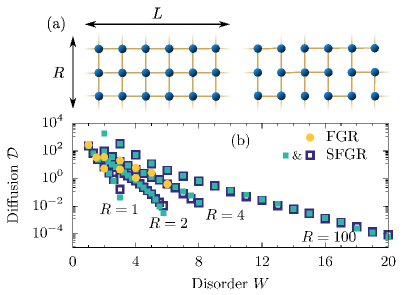
Figure 1: (a) Sketch of the system (left) and percolation problem (right). (b) Diffusion constant ${\cal D}$ obtained from rate equations with Fermi golden rule (FGR) for $L=200$ (circles) and simplified-FGR (SFGR) for $N=LR=10^{4}$ (squares) with various number of legs, $R$, up to a 2D system for $R\gg 1$. Open and filled squares correspond to different realizations of disorder.

Particle in a disordered potential coupled to hard-core bosons– We study a quantum particle on a ladder containing $R$ legs of length $L$ coupled to itinerant hard-core bosons. The system is described by the Hamiltonian Mierzejewski et al. (2019),

$$H = -t\sum_{\langle i,j\rangle}c^{\dagger}_{i}c^{\phantom{\dagger}}_{j}+\sum_{j}\varepsilon_{j}n_{j}+g\sum_{j}n_{j}(a^{\dagger}_{j}+a^{\phantom{\dagger}}_{j})$$ (1)

$$+\omega_{0}\sum_{j}a_{j}^{\dagger}a^{\phantom{\dagger}}_{j}-t_{b}\sum_{\langle i,j\rangle}a_{i}^{\dagger}a^{\phantom{\dagger}}_{j},$$

where $\varepsilon_{j}$ are independent random potentials uniformly distributed in $[-W,W]$. Here, $c^{\dagger}_{j}$ and $a_{j}^{\dagger}$ refer to local fermion and hard-core boson operators ($a^{\dagger}_{j}a^{\dagger}_{j}=0$), respectively. For simplicity, we set $t=1$, $\omega_{0}=g=1$, $t_{b}=0.2$ and restrict our studies to the case of an infinite temperature, $\beta=1/k_{\rm B}T\to 0$.

In order to derive the rate equations (RE), we first diagonalize the single-particle part of the Anderson Hamiltonian [first two terms in Eq. (1)], $H_{\rm SP}=\sum_{l}\epsilon_{l}\varphi_{l}^{\dagger}\varphi_{l}^{\phantom{\dagger}}$, where $\varphi_{l}=\sum_{i}\phi_{li}c_{i}$ and $\phi_{li}$ are single-particle eigen-functions. We then use the FGR to calculate the transition rates $\Gamma_{lk}$ between different $l\neq k$ Anderson states $|l\rangle=\varphi_{l}^{\dagger}|0\rangle$. The emerging RE allow us to study large system sizes $N=LR\lessapprox 10^{3}$, whereas for $N\sim 10^{4}$ we use a simplified FGR (SFGR). In the latter approach, we neglect the momentum dependence of matrix elements for particle-boson interaction and assume a uniform bosonic density of states. In the case of a single chain, the explicit form of $\Gamma_{lk}$ has been derived in Prelovšek et al. (2018) and Mierzejewski et al. (2019) for FGR and SFGR, respectively. For convenience, we recall the main steps of derivations in the Supplemental Material sup .

To directly address the transport, we consider an open system introducing the current source at the left rung and the current drain at the right rung of the ladder, i.e., we study a system with current flowing (on average) along the legs, as described by the RE,

$$\frac{{\rm d}n_{l}}{{\rm d}t}=I_{l}+\sum_{k\neq l}(\Gamma_{kl}n_{k}-\Gamma_{lk}n_{l}).$$ (2)

Here, $n_{l}$ is the occupation of the state $|l\rangle$ and $I_{l}=I^{s}_{l}+I^{d}_{l}$ accounts for the source and the drain, respectively,

$$I^{s}_{l}={\cal I}_{0}\sum_{i\in\rm left}|\phi_{li}|^{2},\quad\quad I^{s}_{d}=-{\cal I}_{0}\sum_{i\in\rm right}|\phi_{li}|^{2},$$ (3)

where the summations are carried out over the left- and right-edge rungs. Since $\phi_{li}$ are normalized, the total injected current $\sum_{l}I^{s}_{l}=R\,{\cal I}_{0}$ hence, ${\cal I}_{0}$ is the average current density. Then, the diffusion constant ${\cal D}$ is obtained from the relation between the current density and the gradient of the particle density, ${\cal D}=-{\cal I}_{0}/\nabla n_{i}$ with $n_{i}=\sum_{l}n_{l}|\phi_{li}|^{2}$ and $n_{l}$ representing the stationary solution of RE (2). We refer to the Supplemental Material sup for technical details on the stationary solution.

Fig. 1(b) shows ${\cal D}$ vs disorder $W$. Each data set corresponds to a single realization of disorder and varying $W$. We also compare results obtained from FGR for $L=200$ and SFGR with much larger $L$. Few things become apparent from the presented results: finite-size effects and sample-to-sample fluctuations are negligible in the diffusive regime; the simplifications introduced within SFGR do not influence the qualitative results. Another evident but nontrivial result is the exponential dependence of ${\cal D}$ on the disorder strength $W$ in a wide range of the latter Barišić and Prelovšek (2010); Prelovšek et al. (2016b); Šuntajs et al. (2019), apparently extending to very large $W$ for the 2D system, $R\gg 1$.

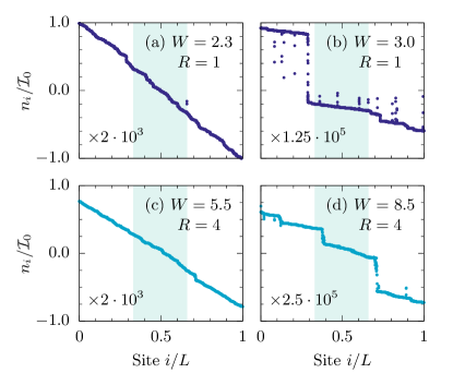
Figure 2: Spatial profiles of $n_{i}$ for $N=10^{4}$. Panels (a), (b) and (c), (d) show results for $R=1$ and $R=4$, respectively. Shaded regions represent sections of the system where the diffusion constant is calculated. Results for $R>1$ are averaged over the rungs.

Results in Fig. 1b are restricted to sufficiently weak disorder when the spatial variation of $n_{i}$ along the legs is linear, as shown in Figs. 2(a) and 2(c). However, for stronger disorder $W\sim W_{c}$, the variation becomes nonlinear due to the formation of weak links which are clearly exemplified in Figs. 2(b) and 2(d). Such behavior signals a transition between the diffusive and subdiffusive regimes. The threshold value $W_{c}$ increases with $R$, but apparently remains finite provided that $R<\infty$. Fig. 1(b) shows also that differences between results for various realizations of disorder Barišić et al. (2016); Khemani et al. (2017) increase upon approaching the transition. Next we demonstrate that the latter sample-to-sample fluctuations are universal for the transition between the diffusive and the subdiffusive regimes.

Sample-to-sample fluctuations– In order to explain the statistical fluctuations of ${\cal D}$, we first consider a strongly disordered single chain ($R=1$) where, for simplicity, the FGR transitions are restricted to Anderson states on neighboring sites, $\Gamma_{kl}\sim\delta_{k,l+1}$, $I^{s}_{l}\simeq{\cal I}_{0}\delta_{l1}$ and $I^{d}_{l}\simeq{\cal I}_{0}\delta_{lL}$. Then, one derives from the stationary solution of Eq. (2) that $n_{l}-n_{l+1}={\cal I}_{0}/\Gamma_{l,l+1}$, and consequently

$$\rho={\cal D}^{-1}\simeq\frac{n_{1}-n_{L}}{L{\cal I}_{0}}=\frac{1}{L}\sum_{l}\tau_{l},\quad\quad\tau_{l}=\frac{1}{\Gamma_{l,l+1}}.$$ (4)

As previously demonstrated for the same model Prelovšek et al. (2018); Mierzejewski et al. (2019), the transition times $\tau_{l}=\Gamma^{-1}_{l,l+1}$, can be well approximated via independent random variables with power-law probability distribution function $f_{\tau}(\tau)\propto\tau^{-(\alpha+1)}$ for large enough $\tau$. Within this simplification, $\rho$ in Eq. (4) becomes an average of $L$-independent random variables with the transition to subdiffusion at $\alpha=1$.

Here, we focus on the diffusive regime, $1<\alpha<2$, where the average transition time is finite $\langle\tau\rangle=\int_{0}^{\infty}{\rm d}\tau\;f_{\tau}(\tau)\tau<\infty$, but $\langle\tau^{2}\rangle$ diverges, thus the fluctuations of $\rho$ are non–Gaussian. It is well established for the fat-tailed (the so-called $\alpha$-stable) distributions Bouchaud and Georges (1989) that the random variable

$$u=\frac{1}{L^{1/\alpha}}\left(\sum_{l=1}^{L}\tau_{l}-L\langle\tau\rangle\right)=L^{(\alpha-1)/\alpha}(\rho-\langle\tau\rangle),$$ (5)

has a limit distribution $f_{u}(u)$ for $L\rightarrow\infty$ and asymptotically $f_{u}(u)\propto u^{-(\alpha+1)}$. Clearly, the latter determines the tails as well as the $L$-dependence of the resistivity distribution $f_{\rho}(\rho)$. In particular, close to the transition to the subdiffusive regime, $\alpha\rightarrow 1$, the exponent in r.h.s. of Eq. (5) vanishes, $(\alpha-1)/\alpha\rightarrow 0$. As a consequence, one obtains weak, at most logarithmic, $L$-dependence of $f_{\rho}(\rho)$. The fat tails can be observed from the cumulative and the complementary cumulative distribution functions of ${\cal D}$ and $\rho$, respectively,

$$F_{\cal D}({\cal D}) = \int_{0}^{{\cal D}}{\rm d}{\cal D}^{\prime}f_{{\cal D}^{\prime}}({\cal D}^{\prime})\simeq\frac{{\cal D}^{\alpha}}{\alpha L^{\alpha-1}},\quad{\cal D}\ll\langle\tau\rangle^{-1},\quad$$ (6)

$$F^{c}_{\rho}(\rho) = \int_{\rho}^{\infty}{\rm d}\rho^{\prime}f_{\rho}(\rho^{\prime})\simeq\frac{1}{\alpha L^{\alpha-1}\rho^{\alpha}},\quad\rho\gg\langle\tau\rangle\,.$$ (7)

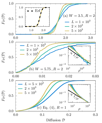
Figure 3: Main panels: cumulative distribution functions of the diffusion constant, $F_{\cal D}({\cal D})$. Inset (a): $F_{\cal D}({\cal D})$ for $L=5\times 10^{3}$ fitted with the error function. Insets (b),(c): complementary distribution functions of the resistivity $F^{c}_{\rho}(\rho)$. (a) and (b) Results obtained via rate equations with SFGR for $R=2$. (c) Results for a chain with independent random transition times with fat-tailed distribution, Eq. (4).

It is by far not clear whether the same properties survive in the considered system, when the transition rates are not independent random variables connecting only neighboring sites but, instead, are obtained fully from FGR. In figures 3a and 3b we present $F_{\cal D}({\cal D})$ (main panels) and $F^{c}_{\rho}(\rho)$ (inset in b) calculated for a two-leg ladder ($R=2$) directly from the stationary solution of Eqs. (2) and with SFGR transition rates. For comparison, we display in Fig. 3c similar results, obtained from the toy model, Eq. (4), with $f_{\tau}(\tau)=\tau^{-(\alpha+1)}$ for $\tau\geq 1$, where we used $\alpha=1.01$. For modest disorder shown in Fig. 3a we confirm that $F_{\cal D}({\cal D})$ represents an error function, in agreement with the Gaussian fluctuations of ${\cal D}$ and its width decreasing approximately as $1/\sqrt{L}$ (not shown). However, upon approaching the transition to the subdiffusive regime, as in Fig. 3b, $F_{\cal D}({\cal D})$ clearly differs from the Gaussian case. Results for $F^{c}_{\rho}(\rho)$ and $F_{\cal D}({\cal D})$ now agree with the analytical predictions, Eqs. (7) and Eqs. (6) for $\alpha\rightarrow 1$. In particular, the statistical fluctuations for $\rho\gg\langle\tau\rangle$ (or ${\cal D}\to 0$) only weakly depend on $L$. Moreover, the latter results are qualitatively similar to those shown in Fig. 3(c) for the toy model ($R=1$) with random transition rates between neighboring Anderson states.

Diffusivity of the planar system– The toy model also offers a simple explanation of why the 2D system remains diffusive for arbitrary $W$, as shown in Fig. 1b. To this end, we construct the lower bound on ${\cal D}$ and demonstrate that it is non-zero. We consider a network with only nearest-neighbor transitions, shown in the right panel of Fig. 1a. We set a threshold transition time $\tau_{\rm th}<\infty$ and check $\tau_{l}$ on each link in the network. For links with $\tau_{l}<\tau_{\rm th}$ we replace $\tau_{l}$ with $\tau_{\rm th}$ and remove links which do not satisfy the latter inequality. As a consequence, the values of all $\tau_{l}$ increase, hence we end up with a percolation problem for a system which obviously has smaller ${\cal D}$ than the original system. The density of removed links $\int_{\tau_{\rm th}}^{\infty}{\rm d}\tau\;f_{\tau}(\tau)=1/(\alpha\tau_{\rm th}^{\alpha})$ may be tuned to an arbitrarily small number via increasing $\tau_{\rm th}$, thus the system may be tuned above the percolation threshold for arbitrary $\alpha>0$. Consequently, the transport is always diffusive.

Fluctuations in disordered spin chains– Next, we check whether such anomalous fluctuations are general and arise also beyond the semi-classical RE approach. To this end, we investigate the sample-to-sample fluctuation of the transport quantities in prototype 1D models which, for strong enough disorder, exhibit MBL or a diffusion-subdiffusion transition.

As a first example, we consider the standard model of MBL, i.e., the Heisenberg model with quenched disorder introduced via a random on-site magnetic field Basko et al. (2006); Oganesyan and Huse (2007). It is commonly accepted that the transition from ergodic to non-ergodic phase takes place at $W/J\simeq 3.7$, where $J$ is the antiferromagnetic exchange coupling Luitz et al. (2015). Furthermore, it has been argued that the MBL phase in this model is preceded by the subdiffusive Griffiths phase Agarwal et al. (2015); Bordia et al. (2017); Agarwal et al. (2016); Lüschen et al. (2017). The second investigated model describes the spin dynamics in the Hubbard chain with a random charge potential. The latter disorder localizes the charge (i.e., the density of fermions), yielding only the spin degrees of freedom mobile. The effective model Kozarzewski et al. (2018); Środa et al. (2019); Kozarzewski et al. (2019); Protopopov et al. (2019) takes a form of the random-exchange ferromagnetic Heisenberg model with a singular distribution of $J$, $f_{J}(J)=\lambda J^{\lambda-1}$ for $0\leqslant J\leqslant 1$. It was shown that for strong charge disorder ($\lambda<1$) the spin dynamics in this specific random-$J$ Heisenberg chain is subdiffusive Kozarzewski et al. (2018); Środa et al. (2019); Kozarzewski et al. (2019). Finally, we examine also the energy transport in the random-transverse-field Ising model for which the existence of MBL has been shown analytically Imbrie (2016b, a).

In order to extract the analogues of the diffusion constant, we calculate the low-frequency regular part of the conductivity ${\cal D}=C(\omega\to 0)$, where $C$ is the spin conductivity in the Heisenberg models and the thermal conductivity in the transverse-field Ising model. It is important to note that the spectrum of a finite-size system with discrete Hilbert space has to be artificially broadened in order to address the d.c. limit. Such broadening can, in principle, affect the value of ${\cal D}$. Our results indicate that although the median, ${\cal D}_{\rm med}$, may substantially dependent on the broadening, the functional form of the distribution $f_{\cal D}({\cal D})$ does not. We refer to the Supplemental Material sup and Ref. Prelovšek and Bonča (2013) for technical details.

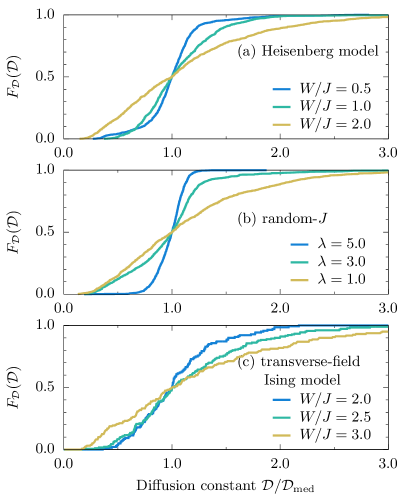
Figure 4: Cumulative distribution functions $F_{\cal D}({\cal D})$ as calculated for various disorder strengths in the ergodic regime for (a) random-field Heisenberg model, (b) random-$J$ Heisenberg model with $f_{J}(J)=\lambda J^{\lambda-1}$ distribution and (c) random-transverse-field Ising model (see the text for details). Panels (a) and (b) are obtained with $N_{r}=1000$ realizations of the disorder, while $N_{r}=200$ in panel (c).

In Fig. 4, we present the cumulative distribution functions $F_{\cal D}({\cal D})$ obtained for the disordered quantum spin chains. For small enough disorder and for all considered models, $F_{\cal D}({\cal D})$ may be well fitted by the error function, reflecting the Gaussian distribution of ${\cal D}$. On the other hand, increasing the disorder strength changes the functional form of $f_{\cal D}({\cal D})$. It is evident that the distributions become non-Gaussian, closely resembling the results in Figs. 3b and 3c for the RE approach. The latter similarity suggests that the fat-tailed fluctuations of resistivity at the diffusion-subdiffusion transition are generic for strongly disordered quasi-1D systems. Due to the limitations of the numerical method, we do not get irrefutable evidence for the spin chains and the latter claim should be considered as a well justified conjecture. The numerical verification of the weak $L$-dependence of $f_{\cal D}({\cal D})$ seems to be a particularly challenging problem.

Conclusions– We have studied how the transport properties of a strongly disordered system with many-body interactions depend on its dimensionality. The geometry of the $R$-leg ladders allowed tuning the system between one-dimensional ($R=1$) and two-dimensional ($R\to\infty$) cases. On the one hand, we have demonstrated that sufficiently strong disorder causes subdiffusive transport for any finite $R$ and that the weak-link scenario survives also for $R>1$. On the other hand, planar systems ($R\to\infty$) appear to be always diffusive, albeit the diffusion constant decreases exponentially with the disorder strength and may eventually become undetectably small. We have shown that the diffusion-subdiffusion transition may be identified via fat-tailed statistical fluctuations of resistivity between different realizations of disorder. Numerical results obtained for various models of disordered spin chains suggest that the latter fluctuations may be generic for quasi-1D quantum systems. The presence of non-Gaussian and almost size–independent fluctuations poses challenging problem for numerical studies, especially when self-averaging quantities are obtained numerically from averaging over various realizations of disorder.

S1 Transition Rates for single particle coupled to hard-core bosons

We recall the main steps of derivations in Prelovšek et al. (2018) and Mierzejewski et al. (2019) for the transition rates between the Anderson states originating from the coupling to hard-core bosons. To this end, we solve the single-particle eigenproblem

$$-t\sum_{\langle i,j\rangle}c^{\dagger}_{i}c^{\phantom{\dagger}}_{j}+\sum_{j}\varepsilon_{j}n_{j}=\sum_{l}\epsilon_{l}\varphi^{\dagger}_{l}\varphi_{l}^{\phantom{\dagger}},$$ (S1)

where $\varphi_{l}^{\dagger}=\sum_{i}\phi_{li}c_{i}^{\dagger}$ creates a particle in the Anderson-localized state with the eigenfunction $\phi_{li}$ and we take all $\phi_{li}$ as real. Then, we rewrite the interaction part of the Hamiltonian using $\varphi_{l}^{\dagger}$

$$H^{\prime} = \sum_{i,l,k}\eta_{lki}\varphi_{l}^{\dagger}\varphi_{k}^{\phantom{\dagger}}(a^{\dagger}_{i}+a_{i}^{\phantom{\dagger}}),\quad\quad\eta_{lki}=g\phi_{ki}\phi_{li}.$$ (S2)

We use the Fermi golden rule (FGR) to calculate the transition rate from $|l\rangle$ to $|k\rangle$

$$\Gamma_{lk} = 2\pi\sum_{b,a}w_{b}|\langle l,b|H^{\prime}|k,a\rangle|^{2}\delta(E_{b,l}-E_{a,k}),$$

$$= \sum_{b}w_{b}\int_{-\infty}^{\infty}{\rm d}t\,\langle l,b|H^{\prime}(t)\left(|k\rangle\langle k|\otimes{\cal I}_{b}\right)H^{\prime}|l,b\rangle,$$

where $|l,b\rangle=|l\rangle\otimes|b\rangle$ and $w_{b}$ are the equilibrium probabilities for finding the hard-core bosons in the state $|b\rangle$. Here, we consider only the case of infinite temperature $T\rightarrow\infty$, hence $w_{b}=\text{const}$.

For hard-core bosons, there may be at most a single boson creation/annihilation per site. Therefore, multi-boson contributions to FGR are significantly reduced with respect to regular bosons. This reduction is particularly important for strong disorder, i.e., for a short localization length of the Anderson states $\phi_{li}$. Neglecting the multi-boson contributions, we rewrite the perturbation using the wave-vector representation for the bosonic operators

$$H^{\prime}(t) \simeq \sum_{lk\bf{q}}\eta_{lk\bf{q}}\varphi_{l}^{\dagger}\varphi_{k}^{\phantom{\dagger}}[a_{-\bf{q}}^{\phantom{\dagger}}e^{it(\epsilon_{l}-\epsilon_{k}-\omega_{\bf{q}})}+a^{\dagger}_{\bf{q}}e^{it(\epsilon_{l}-\epsilon_{k}+\omega_{\bf{q}})}],$$

where

$$\omega_{\bf{q}} = \omega_{0}-2t_{b}[\cos(q_{x})+\cos(q_{y})],$$ (S5)

$$\eta_{lk\bf{q}} = \frac{g}{\sqrt{N}}\sum_{j}e^{-i\bf{q}\cdot\bf{R}_{j}}\phi_{lj}\phi_{kj},$$ (S6)

c.f. Hamiltonian (1) in the main text. At $T\rightarrow\infty$ the hard-core bosons randomly occupy the single-particle states, thus

$$\sum_{b}w_{b}\langle b|a^{\dagger}_{\bf{q}}a^{\phantom{\dagger}}_{\bf{q^{\prime}}}|b\rangle=\sum_{b}w_{b}\langle b|a^{\phantom{\dagger}}_{\bf{q}}a^{\dagger}_{\bf{q^{\prime}}}|b\rangle=\frac{1}{2}\delta_{\bf{q},\bf{q^{\prime}}}$$ (S7)

Substituting Eq. (LABEL:smham2) into (LABEL:smfgr) and using (S7) one finds the transition rates

$$\Gamma_{lk} = \pi\sum_{\bf{q}}|\eta_{lk\bf{q}}|^{2}\left[\delta(\epsilon_{l}-\epsilon_{k}-\omega_{\bf{q}})+\delta(\epsilon_{l}-\epsilon_{k}+\omega_{\bf{q}})\right],$$

which take into account the bosonic dispersion relation and the details of the matrix elements $\eta_{lk\bf{q}}$. In the main text, we refer to Eq. (LABEL:smfgr1) as FGR. Using FGR we study systems up to $N\sim 10^{3}$.

One may significantly simplify the numerical calculations by neglecting the $\bf{q}$-dependence of the matrix elements

$$|\eta_{lk\bf{q}}|^{2}\simeq|\eta_{lk}|^{2}=\frac{1}{N}\sum_{\bf{q}}|\eta_{lk\bf{q}}|^{2}=\frac{g^{2}}{N}\sum_{j}(\phi_{lj}\phi_{kj})^{2},$$ (S9)

and assuming a uniform bosonic density of states

$$\frac{1}{N}\sum_{q}\delta(\omega-\omega_{q})\simeq\frac{1}{\Omega}\theta(\Omega-\omega),\quad\quad\omega\geq 0,$$ (S10)

where $\Omega$ is an effective bosonic frequency. Within these simplifcations the transition rates read

$$\Gamma_{lk} = \pi\frac{g^{2}}{\Omega}\theta(\Omega-|\epsilon_{l}-\epsilon_{k}|)\sum_{j}(\phi_{lj}\phi_{kj})^{2}.$$ (S11)

We refer to Eq. (S11) as the simplified FGR (SFGR) for which we are able to reach $N\sim 10^{4}$. In the numerical calculations we take $\omega_{0}=g=1$ and $t_{b}=0.2$. In the quasi-2D system, the bosonic spectrum has width $8t_{b}$ and the exact density of states is strongly peaked at $\omega=\omega_{0}$. For this reason we take $\Omega=1.2<8t_{b}$.

In order to find the stationary solution of RE (2) in the main text, we put $\frac{{\rm d}n_{l}}{{\rm d}t}=0$ and diagonalize the matrix

$$\widetilde{\Gamma}_{lk} = \delta_{lk}\sum_{j}\Gamma_{lj}-\Gamma_{kl},$$ (S12)

$$\widehat{\widetilde{\Gamma}} = \widehat{U}\;{\rm diag}(\lambda_{1},...\;,\lambda_{N})\;\widehat{U}^{T}.$$ (S13)

Then, one obtains the stationary occupations of the Anderson states

$$n_{l}=\sum_{l,k,j}U_{lj}\frac{1}{\lambda_{j}}U^{T}_{jk}I_{k},$$ (S14)

where we have omitted the zero-mode, $\lambda_{1}=0$, corresponding to the conservation of the total particle number. In order to eliminate the boundary effects, we divide the system into three sections of equal size. The gradient of the particle density in real space, $\nabla n_{i}$, is obtained from the linear fitting of $n_{i}=\sum_{l}n_{l}|\phi_{li}|^{2}$ in the middle section.

S2 Statistical fluctuations of conductivity in disordered spin chains

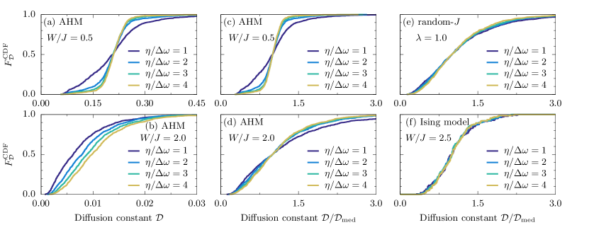
Figure S1: Cumulative distribution functions for the diffusion constant, $F_{\cal D}({\cal D})$, as calculated for various disorder strengths and broadenings $\eta$ for (a-d) random-field Heisenberg model, (e) ferromagnetic random-$J$ Heisenberg model (effective spin Hamiltonian of the Hubbard model with strong disorder in the charge potential), and (f) random transverse-field Ising model (see the text for details).

In the main text of the manuscript, we have considered three one-dimensional quantum spin chains with quenched disorder:

(i) Antiferromagnetic Heisenberg model (AHM)

$$H = J\sum_{i}\left(S^{x}_{i}S^{x}_{i+1}+S^{y}_{i}S^{y}_{i+1}+\Delta S^{z}_{i}S^{z}_{i+1}\right)$$ (S15)

$$+ J\Delta_{2}\sum_{i}S^{z}_{i}S^{z}_{i+2}+\sum_{i}h_{i}\,S^{z}_{i}\,,$$

where we have set $J=1$ as the unit of energy and the local magnetic fields $h_{i}$ are random numbers drawn from a uniform distribution in the interval $h_{i}\in[-W,W]$. Furthermore, we have chosen $\Delta=0.75$ and $\Delta_{2}=0.5$. The latter is the integrability breaking term in the clean limit, $W=0$.

(ii) Ferromagnetic random-$J$ Heisenberg model (effective spin Hamiltonian of the Hubbard model with strong disorder in the charge potential, see Ref. [Kozarzewski et al., 2018] and [Środa et al., 2019] of the main text for more details), i.e.,

$$H = -\sum_{i}J_{i}\,\mathbf{S}_{i}\cdot\mathbf{S}_{i+1}\,.$$ (S16)

Here $\mathbf{S}_{i}$ stands for $\mathbf{S}_{i}=(S^{x}_{i},S^{y}_{i},S^{z}_{i})$ and exchange coupling $J_{i}$ has to be drawn from the probability distribution given by $f_{J}(J)=\lambda J^{\lambda-1}$ for $0\leqslant J\leqslant 1$, where $\lambda$ controls the disorder strength (we refer the interested reader to Ref. [Kozarzewski et al., 2018] and [Środa et al., 2019] of the main text for details on this model).

(iii) Random transverse-field Ising model

$$H=\sum_{i}(J+\delta J_{i})S^{z}_{i}S^{z}_{i+1}+\sum_{i}h_{i}\,S^{z}_{i}+f\sum_{i}\,S^{x}_{i}\,,$$ (S17)

with $J=1$ as the unit of energy, fixed parameter $f/J=0.5$, and uniform distribution $h_{i}\in[-W,W]$. Similarly to the AHM we break the integrability of the clean case ($W=0$), i.e., we added small randomness in the spin exchange coupling, $\delta J_{i}\in[-W_{J},W_{J}]$ with $W_{J}/J=0.2$, thus varying only $W$ in our consideration.

The regular part of the generic conductivity $C(\omega)$ in the high-temperature limit ($\beta\to 0$) can be defined as follows:

$$C_{\mathrm{reg}}(\omega)=\frac{\pi}{LZ}\sum_{E_{n}\neq E_{m}}|\langle n|j|m\rangle|^{2}\,\delta(E_{n}-E_{m}-\omega)\,,$$ (S18)

where $L$ is the considered system size [$L=26$ for the models (i) and (ii); $L=20$ for the model (iii)], $Z$ is the partition function (for $\beta\to 0$, $Z$ is the dimension of the Hilbert space), $|n\rangle$ and $E_{n}$ are the many-body eigenstates and the eigenvalues, respectively. For the Heisenberg models [(i) and (ii)] the diffusion constant was extracted from the spin conductivity ${\cal D}=C_{\mathrm{reg}}(\omega\to 0)=\sigma_{\mathrm{reg}}(\omega\to 0)/\beta$ with the spin current operator defined as $j=j^{S}\equiv\sum_{i}J_{i}\left(S^{x}_{i}S^{y}_{i+1}-S^{y}_{i}S^{x}_{i+1}\right)$. For the transverse-field Ising model (iii) the only conserved quantity is energy. As a consequence, we evaluate the enery (thermal) diffusion constant obtained from the thermal conductivity ${\cal D}=C_{\mathrm{reg}}(\omega\to 0)=\kappa_{\mathrm{reg}}(\omega\to 0)/\beta^{2}$ with the energy current operator defined as $j=j^{E}\equiv f\sum_{i}(J+\delta J_{i})S^{z}_{i}{S}^{x}_{i+1}$. Eq. (S18) is then numerically evaluated with the help of the Microcanonical Lanczos Method Prelovšek and Bonča (2013) with $M_{\mathrm{Lan}}=10^{4}$ Lanczos steps. The latter allows us to obtain frequency resolution $\Delta\omega=\Delta E/M_{\mathrm{Lan}}\simeq 10^{-3}$, where $\Delta E$ is the energy span.

It is important to note that the spectrum in Eq. (S18) is discrete and in order to properly resolve the $\omega\to 0$ limit one has to artificially broaden it with, e.g., the Gaussian kernel,

$$C^{\mathrm{S}}_{\mathrm{reg}}(\omega)=\int\limits_{-\infty}^{\infty}\mathrm{d}\omega^{\prime}\frac{1}{\sqrt{2\pi}\eta}\mathrm{e}^{-\frac{(\omega-\omega^{\prime})^{2}}{2\eta^{2}}}\,C^{\mathrm{R}}_{\mathrm{reg}}(\omega^{\prime})\,,$$ (S19)

where $C^{\mathrm{R}}_{\mathrm{reg}}$ ($C^{\mathrm{S}}_{\mathrm{reg}}$) refers to the raw (smoothed) data. As a consequence, the results—especially in the $\omega\to 0$ limit—can be influenced by the broadening $\eta$. In Fig. S1 we present the cumulative distribution functions of the diffusion constant, $F_{\cal D}({\cal D})$, for all considered models and various values of the broadening $\eta$. It is evident from the presented results that for large disorder, the distribution $F_{\cal D}({\cal D})$ does indeed depend on the value of $\eta$ [see panels (a) and (b)]. However, our results also indicate [panels (c) and (d)] that for any realistic broadening, $\eta>\Delta\omega$, the normalized by median distribution is $\eta$-independent (i.e., the functional form of $F_{\cal D}({\cal D})$ is almost $\eta$-independent) Barišić et al. (2016). Such behavior was observed for all considered models: see panel (e) for the random-$J$ model and panel (f) for the random transverse-field Ising model.