Model Comparison of $\Lambda$CDM vs $R_{h}=ct$ using Cosmic Chronometers

Abstract

In 2012, Bilicki and Seikel Bilicki and Seikel (2012) showed that $H(z)$ data reconstructed using Gaussian Process Regression from cosmic chronometers and baryon acoustic oscillations, conclusively rules out the $R_{h}=ct$ model. These results were disputed by Melia and collaborators in two different works Melia and Maier (2013); Melia and Yennapureddy (2018), who showed using both an unbinned analysis and Gaussian Process reconstructed $H(z)$ data from chronometers, that $R_{h}=ct$ is favored over $\Lambda$CDM model. To resolve this imbroglio, we carry out model comparison of $\Lambda$CDM versus $R_{h}=ct$ by independently reproducing the above claims using the latest chronometer data. We perform model selection between these two models using Bayesian model comparison. We find that no one model between $\Lambda$CDM and $R_{h}=ct$ is decisively favored when uniform priors on $\Lambda$CDM parameters are used. However, if we use priors centered around the Planck best-fit values, then $\Lambda$CDM is very strongly preferred over $R_{h}=ct$.

I Introduction

The standard hot Big-Bang model of cosmology is described by a flat $\Lambda$CDM universe, with 70% of the energy density comprising of the cosmological constant (or any dark energy fluid with equation of state $w\equiv P/\rho$ close to -1) and 25% cold (non-baryonic) dark matter and 5% baryons Peebles and Ratra (2003). This model has two episodes of acceleration (one in the early universe caused by inflation Martin et al. (2014), posited to solve the horizon and flatness problems in the standard hot Big-Bang model Dicke and Peebles (1979)), and another in the late universe, caused by dark energy Huterer and Shafer (2018). This model has been spectacularly confirmed by Planck 2018 CMB observations Aghanim et al. (2018) along with other large-scale structure probes. There are however a few data-driven lingering problems with the standard $\Lambda$CDM paradigm, such as the Hubble constant tension between local and high redshift measurements Verde et al. (2019); Bethapudi and Desai (2017), $\sigma_{8}$ tension between CMB and galaxy clusters Planck Collaboration et al. (2016); Bocquet et al. (2019), Lithium-7 problem in Big-Bang nucleosynthesis Fields et al. (2020), anomalies in CMB at low $l$ Copi et al. (2010), etc. A few works have also challenged some of the most well-established tenets of the standard cosmological model, viz. cosmic acceleration Nielsen et al. (2016) and even cosmic expansion Laviolette (1986).

Independent of the above data driven problems, there are also conceptual problems with the standard model. The best-fit model of scalar-field driven inflation (an essential pillar of standard hot Big-Bang model) with flat potentials also causes lots of fine-tuning issues Ijjas et al. (2014). Furthermore, we don’t yet have laboratory evidence for any cold dark matter candidate, despite searching for over three decades Merritt (2017). If the dark energy turns out to be a cosmological constant, a non-zero value would be very problematic from the point of view of quantum field theory Weinberg (1989); Martin (2012).

Therefore, because of some of the above problems, many alternatives to the standard model have been constructed. One such model is the $R_{h}=ct$ universe model, proposed by Fulvio Melia Melia (2007); Melia and Shevchuk (2012); Melia (2012). In this model, the size of the Hubble sphere given by $R_{h}(t)=ct$ is upheld for all times in contrast to the case of the $\Lambda$CDM model, where this coincidence is true only at the current epoch, i.e. $R_{h}(t_{0})=ct_{0}$. This model has $a(t)\propto t$ and $H(z)=H_{0}(1+z)$. One direct result of this is that the rate of expansion $\dot{a}$ is constant; and pressure and energy density satisfy an equation of state given by $p=-\frac{\rho}{3}$. This is known as the zero active mass condition, and has been argued by Melia to be a necessary requirement due to the symmetries of FRW universes Melia (2016a). (See however Ref. Kim et al. (2016) for objections to this argument of zero active mass condition.) Melia has also argued that this model provides a cosmological basis for the origin of the rest mass energy relation, i.e. $E=mc^{2}$ Melia (2019a), although this has been disputed Lewis (2019). The $R_{h}=ct$ model also has several antecedents and generalizations, discussed in Refs. John (2019); Dev et al. (2002), and an up-to-date review of all such models can be found in Ref. Casado (2020). This model has been tested with a whole slew of cosmological observations by Melia and collaborators; such as cosmic chronometers Melia and Yennapureddy (2018), quasar core angular size measurements Wan et al. (2019), quasar X-ray and UV fluxes Melia (2019b), Type 1a SN Melia et al. (2018), strong lensing Leaf and Melia (2018), cluster gas mass fraction Melia (2016b), etc and found to be in better agreement compared to $\Lambda$CDM model. However, other researchers have reached opposite conclusions and have argued that this model is inconsistent with observations Shafer (2015); Bilicki and Seikel (2012); Lewis et al. (2016); Haridasu et al. (2017); Lin et al. (2018); Hu and Wang (2018); Tu et al. (2019); Fujii (2020). Even before this model was introduced, there were severe observational constraints on power-law cosmologies, within which this model can be subsumed Kaplinghat et al. (1999, 2000). These results in turn have also been contested by Melia and collaborators Melia and McClintock (2015). Conceptual problems have also been raised against this model van Oirschot et al. (2010); Lewis and van Oirschot (2012); Mitra (2014); Lewis (2013a, b); Kim et al. (2016); Bengochea and León (2016), although some have been countered Melia (2018). We note however so far this model is yet to reproduce the Cosmic Microwave Background temperature and polarization anisotropy measurements.

In this work, we try to adjudicate between one such conflicting claim between two of the above works: Ref. Bilicki and Seikel (2012) (BS12, hereafter) and Refs. Melia and Maier (2013); Melia and Yennapureddy (2018) (MM13 and MY18, hereafter), which have reached diametrically opposite conclusions, when analyzing Hubble parameter ($H(z)$) measurements. BS12 reconstructed a non-parametric fit for $H(z)$ using Gaussian Process Regression (GPR hereafter) from 18 cosmic chronometer measurements and 8 BAO measurements spanning the redshift range $0.09\leq z\leq 0.73$. They argued based on a visual inspection of the reconstructed $H(z)$ and its derivatives, that the $\Lambda$CDM model is a much better fit than the $R_{h}=ct$ model. Soon thereafter, MM13 however pointed out that 19 unbinned $H(z)$ measurements obtained from chronometers, support $R_{h}=ct$ over the $\Lambda$CDM. This assertion was based on AIC, BIC, and KIC based tests from information theory and $\chi^{2}$/dof. Most recently, MY18 used 30 $H(z)$ measurements using cosmic chronometers, and similar to BS12, used GPR to reconstruct a non-parametric $H(z)$. Model comparison of $\Lambda$CDM vs $R_{h}=ct$ was done by calculating the normalized area difference between the model and the reconstructed $H(z)$. They argued that with this procedure, $R_{h}=ct$ model is a better fit than $\Lambda$CDM. Here, we do an independent analysis of $H(z)$ data, using the latest measurements from chronometers.

The outline of this paper is as follows. We discuss the GPR technique and Bayesian model comparison technique in Sect. II and Sect. III respectively. The key points made in the two conflicting sets of papers BS12 versus MM13, MY18 are discussed in Sect. IV. The description of our datasets and analysis can be found in Sect. V. Our results using $H(z)$ measurements can be found in Sect. VI. A comparison of the two models using the $Om(z_{1},z_{2})$ statistic can be found in Sect. VII. We conclude in Sect. VIII.

II Gaussian Process Regression

Both the groups (BS12 and MY18) have used GPR for their analysis. Therefore, we provide an abridged introduction to GPR, before discussing the results of their analysis. A more detailed explanation can be found in Section 2 of Ref. Seikel et al. (2012). GPR is a widely used technique in astronomy as it allows us to smoothly interpolate in a non-parametric fashion between different datapoints, thereby allowing us to increase the number of degrees of freedom. However, they do not provide more information than the underlying data. Gaussian process is similar to a Gaussian distribution but it describes the distribution of functions instead of random variables. To describe the distribution of these functions, we need the mean function $\mu(x)$ and a covariance function $cov(f(x),f(\tilde{x}))=k(x,\tilde{x})$ connecting the values of $f$ evaluated at $x$ and $\tilde{x}$. There are many choices for the covariance function. Both the papers have used a squared exponential/Gaussian covariance function, so even in this paper we use a Gaussian kernel for GPR. For a Gaussian kernel $k(x,\tilde{x})$ is:

$$k(x,\tilde{x})=\sigma_{f}^{2}\exp\left(-\frac{(x-\tilde{x})^{2}}{2l^{2}}\right)$$

Here, $\sigma_{f}$ and $l$ are hyper-parameters which describe the ‘bumpiness’ of the function.

Even a random function $f(x)$ can be generated using the covariance matrix. Let $\mathbf{X}$ be the set of points ${x_{i}}$ and one can generate a vector $\mathbf{f^{*}}$ of function values at $\mathbf{X^{*}}$ with $f^{*}_{i}=f(x_{i}^{*})$ as

$$\mathbf{f^{*}}=\mathcal{N}(\mathbf{\mu^{*}},K(\mathbf{X^{*},X^{*}}))$$

The notation $\mathcal{N}$ means that the Gaussian process is evaluated at $x^{*}$, where $f(x^{*})$ is a random value drawn from a normal distribution. Similarly, observational data can be written in the same way as

$$\mathbf{y}=\mathcal{N}(\mathbf{\mu},K(\mathbf{X,X})+C)$$

where $C$ is the covariance matrix of the data. If data is uncorrelated the covariance matrix is simply $diag(\sigma_{i}^{2})$. Using the values of $y$ at $\mathbf{X}$ we can reconstruct $\mathbf{f^{*}}$ using

$$\overline{\mathbf{f^{*}}}=\mathbf{\mu^{*}}+K(\mathbf{X^{*},X})[K(\mathbf{X,X})+C]^{-1}(\mathbf{y-\mu})$$

and

$$cov(\mathbf{f^{*}})=K(\mathbf{X^{*},X^{*}})-K(\mathbf{X^{*},X})[K(\mathbf{X,X})+C]^{-1}K(\mathbf{X,X^{*}})$$

where $\overline{\mathbf{f^{*}}}$ and $cov(\mathbf{f^{*}})$ are mean and covariance of $\mathbf{f^{*}}$ respectively. The diagonal elements of $cov(\mathbf{f^{*}})$ provide us the variance of $\mathbf{f^{*}}$. More details on this can found in Ref. Seikel et al. (2012). Both BS12 and MY18 implement GPR in Python using the package GaPP, which was developed by Seikel and collaborators Seikel et al. (2012).

III Model Comparison summary

Model comparison between two models can be broadly classified into three distinct categories: frequentist, information-theory, and Bayesian techniques Liddle (2004, 2007); Trotta (2017); Shi et al. (2012); Kerscher and Weller (2019). In this work we shall only apply Bayesian model comparison, since this is argued to be the most robust among the different model comparison techniques Trotta (2017); Sharma (2017). We briefly summarize this technique and more details can be found in Refs. Trotta (2017); Kerscher and Weller (2019); Sharma (2017) or some of our previous works Krishak and Desai (2019); Krishak et al. (2020).

Using Bayesian statistics, we compute the probability that the data was generated by each model, also called the Bayesian evidence ($Z$) Trotta (2017):

$$P(\Theta|D,M)=\frac{P(D|\Theta,M)P(\Theta,M)}{P(D|M)}$$ (1)

where $P(\Theta|D,M)$ is the posterior, $P(D|\Theta,M)$ is the likelihood, $P(\Theta,M)$ is the prior, and $P(D|M)$ is the evidence, also sometimes referred to as marginal likelihood. Note that unlike the other model comparison test, the Bayesian evidence does not use the best-fit value of a given model. It considers the entire range. Again, the model with a higher evidence, i.e, higher probability that the data was generated from that model, will be the better model to describe the data. From the Bayesian evidence of the two models, we can calculate the value of the Bayes factor, which is simply the ratio of the evidence for the two models and given by:

$$B=\frac{Z_{1}}{Z_{2}}.$$ (2)

For the Bayes factor, we evaluate the ratio of the evidence of the $\Lambda$CDM to the evidence for the $R_{h}=ct$ model. The significance can be evaluated using the Jeffreys scale Trotta (2017).

IV Summary of BS12, MM13, and MY18

As mentioned in the introduction, there is a large amount of literature comparing the $R_{h}=ct$ model with the $\Lambda$CDM model. We focus on the particular case of these two sets of papers (BS12 versus MM13/MY18) and a few others which only use $H(z)$ measurements, where they have arrived at conflicting results despite similar analysis. We then briefly mention some other works which compared the two models using only expansion history.

BS12 reconstructed the value of the deceleration parameter $q(z)$ from Union2.1 Type 1a Supernova dataset with GPR, and showed from a visual inspection that the reconstructed $q(z)$ better fits the $\Lambda$CDM model. They also used Hubble rate data from 18 cosmic chronometer and 8 BAO measurements, and reconstructed $H(z)$ with GPR, and plotted it against the predicted values of $H(z)$ from the $\Lambda$CDM model and the $R_{h}=ct$ model. They compared the reconstructed $H(z)$, its first and second derivative, as well as the $Om(z)$ diagnostic Sahni et al. (2008) against the theoretical predictions of the two models. They again used visual inspection from these plots to conclude that the $\Lambda$CDM model is a better fit to the data compared to $R_{h}=ct$. Very soon after BS12, MM13 considered 19 unbinned $H(z)$ measurements from cosmic chronometers and fit this data to both the models. They found that the $\chi^{2}$/DOF (or reduced $\chi^{2}$) is equal to 0.745 and 0.777 for $R_{h}=ct$ and $\Lambda$CDM (with parameters given by: $\Omega_{M}=0.32$, $H_{0}=68.9\pm 2.4$ km/sec/Mpc) respectively. Therefore, the reduced $\chi^{2}$ was smaller for $\Lambda$CDM. However, when $\Lambda$CDM model is fit to the cosmic chronometer data, the estimated values of $\Omega_{M}$ and $H_{0}$ (0.27 and $73.8\pm 2.4$ km/sec/Mpc respectively) yield a $\chi^{2}$/DOF of 0.9567, which is greater than that for $R_{h}=ct$ universe. However, no comparison of the goodness of fit based on $\chi^{2}$ p.d.f. was made. They also found smaller values of AIC, BIC, and KIC for $R_{h}=ct$ universe compared to $\Lambda$CDM. However, we note that the difference in information criterion between the two models did not cross the threshold of 10, needed for any one model to be decisively favored over the other. They further criticized the SN data analysis in BS12, arguing that the data used was optimized for $\Lambda$CDM cosmology. They also argued that the BAO data analyzed in BS12 includes non-linear evolution of the matter density and velocity fields, and hence is not model-independent. Therefore, their analysis was done using only chronometers.

A similar analysis using the latest cosmic chronometer data (consisting of 30 measurements) and GPR was carried out in MY18. Here, they used an analytical approach to compare the two models after reconstructing the values of $H(z)$ using GPR. They argued that the $R_{h}=ct$ performs better than the $\Lambda$CDM model, contradicting the conclusion of BS12. To quantify this, they constructed a mock data set using Gaussian random variables, and then computed the normalized absolute area difference between this and the real function. For each model they calculated the differential areas by replacing the mock data set with the predictions from the models, and then estimated the probability of the model ($p$-value). From this analysis they came to the conclusion that the $R_{h}=ct$ model is the better model among the two for the chronometer data.

Besides the above two sets of papers, Ref. Lin et al. (2018) showed using AIC and BIC that a combination of JLA type 1a SN sample and 30 $H(z)$ measurements from chronometers and BAO strongly support the $\Lambda$CDM model over $R_{h}=ct$ universe. They also found using AIC and BIC that the chronometer only measurements by themselves do not decisively favor any one model. Haridasu et al Haridasu et al. (2017) did a joint analysis of Type 1a SN, BAO, GRB and chronometer $H(z)$ data and compared the likelihood of $\Lambda$CDM model with $R_{h}=ct$ using AIC and BIC. They found that both $\Delta$AIC and $\Delta$BIC between the two models is greater than 20, thereby decisively ruling out $R_{h}=ct$ model. Hu and Wang showed from a test of the cosmic distance duality relation using a sample of galaxy clusters and Type 1a SN, that the $\Lambda$CDM model is strongly favored over $R_{h}=ct$ with both $\Delta$AIC and $\Delta$BIC greater than 10 Hu and Wang (2018). Tu et al used a combination of strong lensing, Type 1a supernovae, BAO and cosmic chronometers to argue that $\Lambda$CDM is moderately favored over $R_{h}=ct$ model with the natural logarithm of the Bayes factor greater than five Tu et al. (2019).

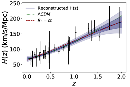
Figure 1: Plot showing $H(z)$ chronometer data along with the best-fit $\Lambda$CDM model and the $R_{h}=ct$ model, with best-fit parameters obtained using unbinned data. Also shown is $H(z)$ reconstructed non-parametrically (along with $1\sigma$ and $2\sigma$ errors in reconstruction). The reconstruction was done with Gaussian Process Regression using the GaPP package.

V Datasets and Analysis

The $H(z)$ data from cosmic chronometers are obtained by comparing relative ages of galaxies at different redshifts and is given by the following expression, assuming an FRW metric Jimenez and Loeb (2002):

$$H(z)=-\frac{1}{1+z}\frac{dz}{dt}$$ (3)

Based on the measurements of the age difference, $\Delta t$, between two passively–evolving galaxies that are separated by a small redshift interval $\Delta z$, we can approximately calculate the value of $dz/dt$ from $\Delta z/\Delta t$. This differential age method is much more reliable than a method based on an absolute age determination for galaxies, as absolute stellar ages are more vulnerable to systematic uncertainties than relative ages.

Even though cosmic chronometers probe only the expansion history of the universe, they have been used for a variety of cosmological inferences, such as determination of $H_{0}$ Chen et al. (2017); Gómez-Valent and Amendola (2018); Yang and Gong (2019); Haridasu et al. (2018), transition redshift from deceleration to acceleration Farooq et al. (2013a); Jesus et al. (2019), cosmic distance duality relation Rana et al. (2017), $\sigma_{8}$ estimation Li et al. (2019), dark energy equation of state Farooq et al. (2013b); Moresco et al. (2016), etc. The complete data set of 31 measurements of $H(z)$ at redshifts $0.07<z<1.965$ from cosmic chronometers is listed in Table 1. This data set was obtained from the compilation in Table III of Ref. Li et al. (2019). A graphical summary of this unbinned data, along with the reconstructed $H(z)$ using GPR can be found in Fig. 1.

Although BS12 (and also Ref. Lin et al. (2018)) has used $H(z)$ measurements from BAO to rule out $R_{h}=ct$ model, we have only used the Hubble parameter data obtained from cosmic chronometers. This is due to various concerns regarding combining data from these two sources for parameter estimation within $\Lambda$CDM and for testing $R_{h}=ct$ universe Zheng et al. (2016); Melia and Maier (2013). One problem in using the BAO data for assessing the viability of an alternative to the $\Lambda$CDM model arises from the fact that measurement of the Hubble parameter from BAO requires the assumption of a particular cosmological model, unlike the model independent measurements of cosmic chronometers. All BAO measurements are scaled by the size of the sound horizon at the drag epoch, $r_{s}$. Computing the value of $r_{s}$ requires the assumption of a fiducial model. Most analyses which employ BAO measurements use the value of $r_{s}$ obtained using the $\Lambda$CDM model. This would induce a bias towards the $\Lambda$CDM model when comparing it with other models. Another concern is that one also needs to model the non-linear evolution of density and velocity fields, which are not model-independent Melia and Maier (2013); Wan et al. (2019). Therefore, in MY18 and MM12, no BAO data was used, whereas both BAO and chronometer data was used in BS12. Accounting for all these problems we present our results for model comparison without the BAO data.

$z$	$H(z)$	$\sigma$	Ref.
	(km/sec/Mpc)	(km/sec/Mpc)
0.07	69	19.6	Zhang et al. (2014)
0.09	69	12	Simon et al. (2005)
0.12	68.6	26.2	Zhang et al. (2014)
0.17	83	8	Simon et al. (2005)
0.179	75	4	Moresco et al. (2011)
0.199	75	5	Moresco et al. (2011)
0.2	72.9	29.6	Zhang et al. (2014)
0.27	77	14	Simon et al. (2005)
0.28	88.8	36.6	Zhang et al. (2014)
0.352	83	14	Moresco et al. (2011)
0.3802	83	13.5	Moresco et al. (2016)
0.4	95	17	Simon et al. (2005)
0.4004	77	10.2	Moresco et al. (2016)
0.4247	87.1	11.2	Moresco et al. (2016)
0.4497	92.8	12.9	Moresco et al. (2016)
0.47	89	34	Ratsimbazafy et al. (2017)
0.4783	80.9	9	Moresco et al. (2016)
0.48	97	62	Stern et al. (2010)
0.593	104	13	Moresco et al. (2011)
0.68	92	8	Moresco et al. (2011)
0.781	105	12	Moresco et al. (2011)
0.875	125	17	Moresco et al. (2011)
0.88	90	40	Stern et al. (2010)
0.9	117	23	Simon et al. (2005)
1.037	154	20	Moresco et al. (2011)
1.3	168	17	Simon et al. (2005)
1.363	160	33.6	Moresco (2015)
1.43	177	18	Simon et al. (2005)
1.53	140	14	Simon et al. (2005)
1.75	202	40	Simon et al. (2005)
1.965	186.5	50.4	Moresco (2015)

Table 1: $H(z)$ data from cosmic chronometers along with references to original sources. This list was compiled from Ref. Li et al. (2019).

The first step in model comparison is to find the best-fit values of the free parameters in $\Lambda$CDM as well as the $R_{h}=ct$ universe model. This is obtained by minimizing the $\chi^{2}$ functional given by:

$$\chi^{2}=\sum_{i=1}^{N}\left(\frac{H_{i}(z)-H^{\Lambda CDM/R_{h}=ct}(z,\theta)}{\sigma_{i}}\right)^{2},$$ (4)

where $H_{i}(z)$ indicate the various Hubble parameter measurements, $N$ is the total number of datapoints used, $H^{\Lambda CDM/R_{h}=ct}(z,\theta)$ encapsulates the relation for the Hubble parameter in $\Lambda$CDM and $R_{h}=ct$ cosmology; $\sigma_{i}$ denotes the error in $H(z)$; and $\theta$ denotes the parameter vector in the two models.

In the $R_{h}=ct$ model, $H(z)$ is given by:

$$H(z)=H_{0}(1+z),$$ (5)

whereas for the the $\Lambda$CDM model, $H(z)$ is:

$$H(z)=H_{0}\sqrt{\Omega_{M}(1+z)^{3}+(1-\Omega_{M}-\Omega_{\Lambda})(1+z)^{2}+\Omega_{\Lambda}}$$ (6)

where $\Omega_{M}$ and $\Omega_{\Lambda}$ are the density parameters of matter and the cosmological constant respectively. Note that for a flat $\Lambda$CDM model, $\Omega_{\Lambda}=1-\Omega_{M}$, which reduces the number of free parameters by one. For a flat $\Lambda$CDM model the equation would be -

$$H(z)=H_{0}\sqrt{\Omega_{M}(1+z)^{3}+1-\Omega_{M}}$$ (7)

In both BS12 and MM13, a flat $\Lambda$CDM model was used for the model comparison. So in this work we will stick to the flat case of the $\Lambda$CDM model ($\Omega_{k}=0$) with $H(z)$ given from equation 7.

Since Bayesian model comparison does not depend upon the best-fit values, we do not have to maximize any likelihood. We only need to choose priors for the two models. For $\Lambda$CDM, we used two sets of priors. The first set assumes a uniform distribution for $\Omega_{M}$ and $H_{0}$. For the second set of priors, we use the 2018 Planck cosmology determined best-fit parameters Aghanim et al. (2018), and choose Gaussian priors centered around these values. The $R_{h}=ct$ universe has only one free parameter, $H_{0}$ and we used the same (uniform) $H_{0}$ prior as in $\Lambda$CDM model. A summary of all the priors used for model comparison for both the models can be found in Table 2. In this work, the Bayesian evidence was computed using the dynesty Speagle (2020) package, which uses the nested sampling technique.

VI Results

We now present our results for model comparison using the chronometer dataset. We carried out two different analyses. The first analysis involves using the unbinned data. The second analysis involves reconstructing $H(z)$ using the non-parametric GPR method. For each of these datasets, we used two different priors for $\Lambda$CDM, as outlined in the previous section. For this purpose, we repeat the analysis done in BS12, wherein $H(z)$ is reconstructed at many values using GPR. The GPR was done using the GaPP software. This GPR reconstructed $H(z)$ for chronometers along with the original unbinned measurements is shown in Fig. 1, along with the best-fit $\Lambda$CDM model and the $R_{h}=ct$ model. For carrying out model comparison with GPR, we use 100 reconstructed measurements uniformly distributed between the lowest and highest available redshift.

VI.1 Model comparison using unbinned data

Our model comparison results using unbinned analysis using both the prior choices are summarized in Table 3. The summary of these results is as follows. When uniform priors for $\Lambda$CDM are chosen, the Bayes factor (defined as ratio of Bayesian evidence for $\Lambda$CDM model to $R_{h}=ct$) is close to one, and hence does not prefer any one model over the other. However, if we choose Gaussian priors centered around Planck best-fit values, then $\Lambda$CDM is very strongly favored over $R_{h}=ct$ using Jeffreys scale. Therefore, we disagree with MM12 that $R_{h}=ct$ is favored, if you consider only chronometer data.

VI.2 Model Comparison using GPR data

Our results for model comparison using data reconstructed with GPR can be found in Tables 4. The Bayes factor again marginally favors $\Lambda$CDM, when uniform priors are used. When we use Planck based priors, then $\Lambda$CDM is decisively favored over $R_{h}=ct$.

Therefore, in summary we disagree with MS18 that $R_{h}=ct$ provides a better fit than the $\Lambda$CDM model, since no test provides a decisive evidence for either model and most tests strongly favor the $\Lambda$CDM model. At the same time we note that out $R_{h}=ct$ model cannot be currently ruled out using chronometers, if we use uniform priors on $\Omega_{M}$ and $H_{0}$.

$\Lambda$CDM - Uniform prior
$\Omega_{M}$	$\mathcal{U}(0,1)$
$H_{0}$	$\mathcal{U}(0,100)$
$\Lambda$CDM - Gaussian prior
$\Omega_{M}$	$\mathcal{N}(0.315,0.007)$
$H_{0}$	$\mathcal{N}(67.4,0.5)$
$R_{h}=ct$
$H_{0}$	$\mathcal{U}(0,100)$

Table 2: The priors used for the analysis. $\mathcal{U}(x,y)$ denotes a top-hat or a uniform prior between $x$ and $y$. $\mathcal{N}(x,y)$ denotes a Gaussian prior with a mean of $x$ and scale parameter of $y$. The Gaussian priors for $\Lambda$CDM are centered around the best fit values of the 2018 results of Planck collaboration Aghanim et al. (2018), with the scale parameter equal to $1\sigma$ error of these results. The priors on $H_{0}$ are given in units of km/sec/Mpc

	$R_{h}=ct$	$\Lambda$CDM	$\Lambda$CDM
		(Uniform Prior)	(Gaussian prior)
$\log Z$	-128.0	-129.3	-123.9
Bayes Factor	-	0.3	60.0

Table 3: Comparison of Bayes factor for $R_{h}=ct$ and $\Lambda$CDM using unbinned measurements of chronometer data listed in Table 1, using two different sets of priors in $\Lambda$CDM (cf. Table 2) $\log Z$ denotes the logarithm of the Bayesian evidence. The Bayes factor is defined as the ratio of the evidence of the $\Lambda$CDM model to the evidence for the $R_{h}=ct$ universe model. When uniform priors are used for $\Lambda$CDM, the Bayesian evidence for the two models are almost identical, with no one model been preferred. When we used Gaussian priors centered on the Planck best-fit values Aghanim et al. (2018), $\Lambda$CDM is very strongly preferred over $R_{h}=ct$.

	$R_{h}=ct$	$\Lambda$CDM	$\Lambda$CDM
		(Uniform Prior)	(Gaussian prior)
$\log Z$	-277.7	-277.3	-270.8
Bayes Factor	-	1.6	992.3

Table 4: Model Comparison tests using GPR measurements of chronometer data listed in Table 1. The explanation of all the columns is the same as in Table 3. When uniform priors are used, no one model is preferred, whereas $\Lambda$CDM is decisively favored if we use Gaussian priors obtained from the 2018 Planck best-fit measurements Aghanim et al. (2018)

VII Diagnosis using $Om$ statistic

We now explore if we can distinguish between the two models using the two-point $Om(z_{1},z_{2})$ statistic between any two pairs of redshifts ($z_{1}$,$z_{2}$). The $Om(z_{1},z_{2})$ statistic is defined as Shafieloo et al. (2012):

$$Om(z1,z2)=\frac{h^{2}(z_{1})-h^{2}(z_{2})}{(1+z_{1})^{3}-(1+z_{2})^{3}}$$ (8)

where $h(z)=H(z)/H_{0}$. The $Om(z_{1},z_{2})$ statistic has been used to map out the expansion history of the universe and also as a null test of $\Lambda$CDM in a number of works Shafieloo et al. (2012); Sahni et al. (2014); Qi et al. (2018); Cao et al. (2018); Escamilla-Rivera and Fabris (2016); Zheng et al. (2016). For $\Lambda$CDM model, $Om(z_{1},z_{2})$ has the remarkable property that it is independent of $z_{1}$ and $z_{2}$, and is equal to $\Omega_{M}$ Sahni et al. (2014). Therefore, computing the $Om(z_{1},z_{2})$ using $H(z)$ measurements enables us to carry out a model independent test of $\Lambda$CDM and simultaneously obtain an estimate of $\Omega_{M}$. For $R_{h}=ct$ universe, $Om(z1,z2)$ is given by

$$Om^{R_{h}=ct}=\frac{(1+z_{1})^{2}-(1+z_{2})^{2}}{(1+z_{1})^{3}-(1+z_{2})^{3}}$$ (9)

Therefore for $R_{h}=ct$ model, $Om(z1,z2)$ is not a constant and is a function of $z_{1}$ and $z_{2}$.

From 31 $H(z)$ measurements, we obtain a total of ${}^{31}C_{2}$ or 465 $Om(z_{1},z_{2})$ data points. These data points can be found in Fig. 2. The errors are obtained from Gaussian error propagation from the errors in $H(z_{1})$ and $H(z_{2})$. As we can see, for low values of the redshift difference, the errors in $Om(z_{1},z_{2})$ are quite large, and although they reduce with increasing $z_{2}-z_{1}$, they are usually of the same order as $Om(z_{1},z_{2})$.

For doing model comparison, we need to determine the total number of free parameters in $\Lambda$CDM and $R_{h}=ct$. For $\Lambda$CDM, this is equal to one, since $H_{0}$ is degenerate with $\Omega_{m}$, and choosing a different $H_{0}$ would lead to a different $\Omega_{m}$. However, irrespective of which value of $H_{0}$ is used, $Om(z1,z2)$ would be a constant, independent of the redshift difference. Since $Om(z1,z2)$ is constant for $\Lambda$CDM model, the best-fit maximum likelihood estimate would just be the weighted mean of all the $Om(z1,z2)$ measurements. For $R_{h}=ct$, the only free parameter would be $H_{0}$, since varying $H_{0}$ would vertically re-scale the whole plot by a constant offset.

For $\Lambda$CDM, we get

$$\chi^{2}/dof=185.4/350$$

and for $R_{h}=ct$ we get

$$\chi^{2}/dof=185.2/350$$

For doing this fit, we removed four $H(z)$ points with the largest error bars. So the total number of $Om(z_{1},z_{2})$ data points used for doing the fits is equal to 351. As we see, both the $\chi^{2}/dof$ values are smaller than one and are very close to each other making the $Om(z_{1},z_{2})$ ineffective for this model comparison. For illustrative purposes, we show this best-fit along with some of the $Om(z_{1},z_{2})$ (after removing the error bars) in Fig. 3. Therefore, it is not possible to distinguish between the two models using current $H(z)$ chronometer data.

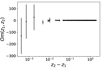
Figure 2: Plot of $Om(z_{1},z_{2})$ calculated from the chronometer data using equation 8. These points were calculated from combinations of the 31 Hubble measurements in pairs, amounting to 465 points. The theoretical plots are not included because the theoretical curves cannot be distinguished at this scale.

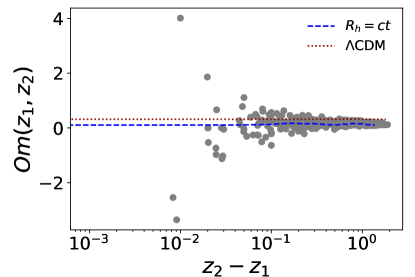
Figure 3: This plot shows the theoretical curves for the best-fit $\Lambda$CDM and $R_{h}=ct$ models , along with the data for $Om(z_{1},z_{2})$ (grey points). For this plot, four $H(z)$ points with the largest error bars have been removed for which the value of $Om(z_{1},z_{2})$ was large. Since this plot is for illustrative purposes, we have also removed the error bars in the $Om(z_{1},z_{2})$ values for brevity. The actual error bars are much larger than the differences between the two models. Therefore, it is not possible to distinguish between the two models using $Om(z_{1},z_{2})$ measurements.

VIII Conclusions

In this work we try to independently assess the viability of $\Lambda$CDM vs $R_{h}=ct$ universe using only $H(z)$ measurements from cosmic chronometers to resolve conflicting claims between two groups of authors. In 2012, Bilicki and Seikel Bilicki and Seikel (2012) claimed using $H(z)$ measurements from chronometers and BAO, that $R_{h}=ct$ model is conclusively ruled out. This was contested by Melia and collaborators  Melia and Maier (2013); Melia and Yennapureddy (2018), who showed using $H(z)$ measurements from chronometers that $R_{h}=ct$ universe is favored over $\Lambda$CDM. They also pointed out BAO measurements cannot be used to test $R_{h}=ct$ models, since the BAO $H(z)$ measurements implicitly assume $\Lambda$CDM. A few other works Shafer (2015); Lin et al. (2018); Haridasu et al. (2017); Tu et al. (2019) also found that type 1a SN, $H(z)$ measurements from chronometers, and BAO rule out $R_{h}=ct$ model.

In order to settle the conflicting results between the above two groups of authors, we considered measurements from only chronometers (to emulate the analysis in Ref. Melia and Maier (2013); Melia and Yennapureddy (2018)).) We did not consider the BAO measurements, given the circularity involved in using them for testing non-$\Lambda$CDM universes Melia and Maier (2013); Melia and Yennapureddy (2018). We carried out model comparison using both the unbinned data, and also by doing a non-parametric reconstruction using GPR. To carry out model comparison, we used a Bayesian model comparison technique by computing the Bayes factor between the two models. We used two different priors for the $\Lambda$CDM: a uniform prior over a wide parameter range, and also Gaussian priors centered around the 2018 Planck best-fit $\Lambda$CDM cosmology. A summary of these priors used can be found in Table 2.

Our results for both these priors and datasets can be found in Tables 3 and  4. When we use a uniform prior, the difference in significance between the two models is negligible, using both the datasets. However, for the priors centered around the Planck 2018 best-fit $\Lambda$CDM values, we find that $\Lambda$CDM is very strongly/decisively favored over $R_{h}=ct$ for the unbinned/GPR reconstructed datasets. Therefore, we conclude that using the chronometer $H(z)$ data, $R_{h}=ct$ model is not preferred over $\Lambda$CDM.

We also investigated if the $Om$ statistic, calculated using redshift pairs, which has been used in previous literature for testing $\Lambda$CDM model Shafieloo et al. (2012); Sahni et al. (2014), can be used to discriminate between the two models. Unfortunately, the current error bars in $Om(z_{1},z_{2})$ estimated using chronometer $H(z)$ data are too large to enable a robust model comparison.

Therefore, in summary, we disagree with the claims in both Ref. Bilicki and Seikel (2012) and Ref. Melia and Maier (2013); Melia and Yennapureddy (2018), and conclude that neither model is ruled out or decisively favored using only $H(z)$ measurements with chronometers, if we use uniform priors on parameters of both models. A more acid test would be using CMB and other large scale structure based tests in a theory-independent fashion.

References

- Bilicki and Seikel (2012) M. Bilicki and M. Seikel, Mon. Not. R. Astron. Soc. 425, 1664 (2012), eprint 1206.5130.
- Melia and Maier (2013) F. Melia and R. S. Maier, Mon. Not. R. Astron. Soc. 432, 2669 (2013), eprint 1304.1802.
- Melia and Yennapureddy (2018) F. Melia and M. K. Yennapureddy, JCAP 2018, 034 (2018), eprint 1802.02255.
- Peebles and Ratra (2003) P. J. Peebles and B. Ratra, Reviews of Modern Physics 75, 559 (2003), eprint astro-ph/0207347.
- Martin et al. (2014) J. Martin, C. Ringeval, and V. Vennin, Physics of the Dark Universe 5, 75 (2014), eprint 1303.3787.
- Dicke and Peebles (1979) R. H. Dicke and P. J. E. Peebles, in General Relativity: An Einstein Centenary Survey (1979).
- Huterer and Shafer (2018) D. Huterer and D. L. Shafer, Reports on Progress in Physics 81, 016901 (2018), eprint 1709.01091.
- Aghanim et al. (2018) N. Aghanim et al. (Planck) (2018), eprint 1807.06209.
- Verde et al. (2019) L. Verde, T. Treu, and A. G. Riess, Nature Astronomy 3, 891 (2019), eprint 1907.10625.
- Bethapudi and Desai (2017) S. Bethapudi and S. Desai, Eur. Phys. J. Plus 132, 78 (2017), eprint 1701.01789.
- Planck Collaboration et al. (2016) Planck Collaboration, P. A. R. Ade, N. Aghanim, M. Arnaud, M. Ashdown, J. Aumont, C. Baccigalupi, A. J. Banday, R. B. Barreiro, J. G. Bartlett, et al., Astron. & Astrophys. 594, A24 (2016), eprint 1502.01597.
- Bocquet et al. (2019) S. Bocquet, J. P. Dietrich, T. Schrabback, L. E. Bleem, M. Klein, S. W. Allen, D. E. Applegate, M. L. N. Ashby, M. Bautz, M. Bayliss, et al., Astrophys. J. 878, 55 (2019), eprint 1812.01679.
- Fields et al. (2020) B. D. Fields, K. A. Olive, T.-H. Yeh, and C. Young, JCAP 2020, 010 (2020), eprint 1912.01132.
- Copi et al. (2010) C. J. Copi, D. Huterer, D. J. Schwarz, and G. D. Starkman, Adv. Astron. 2010, 847541 (2010), eprint 1004.5602.
- Nielsen et al. (2016) J. T. Nielsen, A. Guffanti, and S. Sarkar, Scientific Reports 6, 35596 (2016), eprint 1506.01354.
- Laviolette (1986) P. A. Laviolette, Astrophys. J. 301, 544 (1986).
- Ijjas et al. (2014) A. Ijjas, P. J. Steinhardt, and A. Loeb, Physics Letters B 736, 142 (2014), eprint 1402.6980.
- Merritt (2017) D. Merritt, Studies in the History and Philosophy of Modern Physics 57, 41 (2017), eprint 1703.02389.
- Weinberg (1989) S. Weinberg, Reviews of Modern Physics 61, 1 (1989).
- Martin (2012) J. Martin, Comptes Rendus Physique 13, 566 (2012), eprint 1205.3365.
- Melia (2007) F. Melia, Mon. Not. R. Astron. Soc. 382, 1917 (2007), eprint 0711.4181.
- Melia and Shevchuk (2012) F. Melia and A. Shevchuk, Mon. Not. Roy. Astron. Soc. 419, 2579 (2012), eprint 1109.5189.
- Melia (2012) F. Melia, Austral. Physics 49, 83 (2012), eprint 1205.2713.
- Melia (2016a) F. Melia, Frontiers of Physics 11, 119801 (2016a), eprint 1601.04991.
- Kim et al. (2016) D. Y. Kim, A. N. Lasenby, and M. P. Hobson, Mon. Not. R. Astron. Soc. 460, L119 (2016), eprint 1601.07890.
- Melia (2019a) F. Melia, International Journal of Modern Physics A 34, 1950055 (2019a), eprint 1904.04651.
- Lewis (2019) G. F. Lewis, General Relativity and Gravitation 51, 119 (2019), eprint 1908.09267.
- John (2019) M. V. John, Mon. Not. R. Astron. Soc. 484, L35 (2019), eprint 1902.05088.
- Dev et al. (2002) A. Dev, M. Safonova, D. Jain, and D. Lohiya, Physics Letters B 548, 12 (2002), eprint astro-ph/0204150.
- Casado (2020) J. Casado, Astrophys. and Space Science 365, 16 (2020).
- Wan et al. (2019) H.-Y. Wan, S.-L. Cao, F. Melia, and T.-J. Zhang, Physics of the Dark Universe 26, 100405 (2019), eprint 1910.14024.
- Melia (2019b) F. Melia, Mon. Not. R. Astron. Soc. 489, 517 (2019b), eprint 1907.13127.
- Melia et al. (2018) F. Melia, J. J. Wei, R. S. Maier, and X. F. Wu, EPL (Europhysics Letters) 123, 59002 (2018), eprint 1809.05094.
- Leaf and Melia (2018) K. Leaf and F. Melia, Mon. Not. R. Astron. Soc. 478, 5104 (2018), eprint 1805.08640.
- Melia (2016b) F. Melia, Proceedings of the Royal Society of London Series A 472, 20150765 (2016b), eprint 1601.04649.
- Shafer (2015) D. L. Shafer, Phys. Rev. D 91, 103516 (2015), eprint 1502.05416.
- Lewis et al. (2016) G. F. Lewis, L. A. Barnes, and R. Kaushik, Mon. Not. R. Astron. Soc. 460, 291 (2016), eprint 1604.07460.
- Haridasu et al. (2017) B. S. Haridasu, V. V. Luković, R. D’Agostino, and N. Vittorio, Astron. & Astrophys. 600, L1 (2017), eprint 1702.08244.
- Lin et al. (2018) H.-N. Lin, X. Li, and Y. Sang, Chinese Physics C 42, 095101 (2018), eprint 1711.05025.
- Hu and Wang (2018) J. Hu and F. Y. Wang, Mon. Not. R. Astron. Soc. 477, 5064 (2018), eprint 1804.06606.
- Tu et al. (2019) Z. L. Tu, J. Hu, and F. Y. Wang, Mon. Not. R. Astron. Soc. 484, 4337 (2019), eprint 1901.09144.
- Fujii (2020) H. Fujii, Research Notes of the American Astronomical Society 4, 72 (2020).
- Kaplinghat et al. (1999) M. Kaplinghat, G. Steigman, I. Tkachev, and T. P. Walker, Phys. Rev. D 59, 043514 (1999), eprint astro-ph/9805114.
- Kaplinghat et al. (2000) M. Kaplinghat, G. Steigman, and T. P. Walker, Phys. Rev. D 61, 103507 (2000), eprint astro-ph/9911066.
- Melia and McClintock (2015) F. Melia and T. M. McClintock, Astron. J. 150, 119 (2015), eprint 1507.08279.
- van Oirschot et al. (2010) P. van Oirschot, J. Kwan, and G. F. Lewis, Mon. Not. R. Astron. Soc. 404, 1633 (2010), eprint 1001.4795.
- Lewis and van Oirschot (2012) G. F. Lewis and P. van Oirschot, Mon. Not. R. Astron. Soc. 423, L26 (2012), eprint 1203.0032.
- Mitra (2014) A. Mitra, Mon. Not. Roy. Astron. Soc. 442, 382 (2014).
- Lewis (2013a) G. F. Lewis, Mon. Not. R. Astron. Soc. 431, L25 (2013a), eprint 1301.0305.
- Lewis (2013b) G. F. Lewis, Mon. Not. R. Astron. Soc. 432, 2324 (2013b), eprint 1304.1248.
- Bengochea and León (2016) G. R. Bengochea and G. León, European Physical Journal C 76, 626 (2016), eprint 1606.08803.
- Melia (2018) F. Melia, American Journal of Physics 86, 585 (2018), eprint 1807.07587.
- Seikel et al. (2012) M. Seikel, C. Clarkson, and M. Smith, JCAP 1206, 036 (2012), eprint 1204.2832.
- Liddle (2004) A. R. Liddle, Mon. Not. Roy. Astron. Soc. 351, L49 (2004), eprint astro-ph/0401198.
- Liddle (2007) A. R. Liddle, Mon. Not. Roy. Astron. Soc. 377, L74 (2007), eprint astro-ph/0701113.
- Trotta (2017) R. Trotta, arXiv e-prints arXiv:1701.01467 (2017), eprint 1701.01467.
- Shi et al. (2012) K. Shi, Y. F. Huang, and T. Lu, Mon. Not. R. Astron. Soc. 426, 2452 (2012), eprint 1207.5875.
- Kerscher and Weller (2019) M. Kerscher and J. Weller, SciPost Physics Lecture Notes 9 (2019), eprint 1901.07726.
- Sharma (2017) S. Sharma, Ann. Rev. Astron. Astrophys. 55, 213 (2017), eprint 1706.01629.
- Krishak and Desai (2019) A. Krishak and S. Desai, Open J. Astrophys. (2019), eprint 1907.07199.
- Krishak et al. (2020) A. Krishak, A. Dantuluri, and S. Desai, JCAP 2002, 007 (2020), eprint 1906.05726.
- Sahni et al. (2008) V. Sahni, A. Shafieloo, and A. A. Starobinsky, Phys. Rev. D78, 103502 (2008), eprint 0807.3548.
- Jimenez and Loeb (2002) R. Jimenez and A. Loeb, Astrophys. J. 573, 37 (2002), eprint astro-ph/0106145.
- Chen et al. (2017) Y. Chen, S. Kumar, and B. Ratra, Astrophys. J. 835, 86 (2017), eprint 1606.07316.
- Gómez-Valent and Amendola (2018) A. Gómez-Valent and L. Amendola, JCAP 2018, 051 (2018), eprint 1802.01505.
- Yang and Gong (2019) Y. Yang and Y. Gong, arXiv e-prints arXiv:1912.07375 (2019), eprint 1912.07375.
- Haridasu et al. (2018) B. S. Haridasu, V. V. Luković, M. Moresco, and N. Vittorio, JCAP 2018, 015 (2018), eprint 1805.03595.
- Farooq et al. (2013a) O. Farooq, S. Crandall, and B. Ratra, Physics Letters B 726, 72 (2013a), eprint 1305.1957.
- Jesus et al. (2019) J. F. Jesus, R. Valentim, A. A. Escobal, and S. H. Pereira, arXiv e-prints arXiv:1909.00090 (2019), eprint 1909.00090.
- Rana et al. (2017) A. Rana, D. Jain, S. Mahajan, A. Mukherjee, and R. F. L. Holanda, JCAP 2017, 010 (2017), eprint 1705.04549.
- Li et al. (2019) E.-K. Li, M. Du, Z.-H. Zhou, H. Zhang, and L. Xu, arXiv e-prints arXiv:1911.12076 (2019), eprint 1911.12076.
- Farooq et al. (2013b) O. Farooq, D. Mania, and B. Ratra, Astrophys. J. 764, 138 (2013b), eprint 1211.4253.
- Moresco et al. (2016) M. Moresco, R. Jimenez, L. Verde, A. Cimatti, L. Pozzetti, C. Maraston, and D. Thomas, JCAP 2016, 039 (2016), eprint 1604.00183.
- Li et al. (2019) E. K. Li, M. Du, Z. H. Zhou, H. Zhang, and L. Xu, arXiv preprint arXiv:1911.12076 (2019).
- Zheng et al. (2016) X. Zheng, X. Ding, M. Biesiada, S. Cao, and Z. Zhu, Astrophys. J. 825, 17 (2016), eprint 1604.07910.
- Zhang et al. (2014) C. Zhang, H. Zhang, S. Yuan, T.-J. Zhang, and Y.-C. Sun, Res. Astron. Astrophys. 14, 1221 (2014), eprint 1207.4541.
- Simon et al. (2005) J. Simon, L. Verde, and R. Jimenez, Phys. Rev. D71, 123001 (2005), eprint astro-ph/0412269.
- Moresco et al. (2011) M. Moresco, R. Jimenez, A. Cimatti, and L. Pozzetti, JCAP 1103, 045 (2011), eprint 1010.0831.
- Ratsimbazafy et al. (2017) A. L. Ratsimbazafy, S. I. Loubser, S. M. Crawford, C. M. Cress, B. A. Bassett, R. C. Nichol, and P. Väisänen, Mon. Not. Roy. Astron. Soc. 467, 3239 (2017), eprint 1702.00418.
- Stern et al. (2010) D. Stern, R. Jimenez, L. Verde, M. Kamionkowski, and S. A. Stanford, JCAP 1002, 008 (2010), eprint 0907.3149.
- Moresco (2015) M. Moresco, Mon. Not. Roy. Astron. Soc. 450, L16 (2015), eprint 1503.01116.
- Speagle (2020) J. S. Speagle, Mon. Not. R. Astron. Soc. (2020), eprint 1904.02180.
- Shafieloo et al. (2012) A. Shafieloo, V. Sahni, and A. A. Starobinsky, Phys. Rev. D 86, 103527 (2012), eprint 1205.2870.
- Sahni et al. (2014) V. Sahni, A. Shafieloo, and A. A. Starobinsky, Astrophys. J. Lett. 793, L40 (2014), eprint 1406.2209.
- Qi et al. (2018) J.-Z. Qi, S. Cao, M. Biesiada, T.-P. Xu, Y. Wu, S.-X. Zhang, and Z.-H. Zhu, Research in Astronomy and Astrophysics 18, 066 (2018), eprint 1803.04109.
- Cao et al. (2018) S.-L. Cao, X.-W. Duan, X.-L. Meng, and T.-J. Zhang, European Physical Journal C 78, 313 (2018), eprint 1712.01703.
- Escamilla-Rivera and Fabris (2016) C. Escamilla-Rivera and J. Fabris, Galaxies 4, 76 (2016), eprint 1511.07066.