NewsStand CoronaViz: A Map Query Interface for Spatio-Temporal and Spatio-Textual Monitoring of Disease Spread

Abstract

With the rapid continuing spread of COVID-19, it is clearly important to be able to track the progress of the virus over time in order to be better prepared to anticipate its emergence and spread in new regions as well as declines in its presence in regions thereby leading to or justifying “reopening” decisions. There are many applications and web sites that monitor officially released numbers of cases which are likely to be the most accurate methods for tracking the progress of the virus; however, they will not necessarily paint a complete picture. To begin filling any gaps in official reports, we have developed the NewsStand CoronaViz web application (https://coronaviz.umiacs.io) that can run on desktops and mobile devices that allows users to explore the geographic spread in discussions about the virus through analysis of keyword prevalence in geotagged news articles and tweets in relation to the real spread of the virus as measured by confirmed case numbers reported by the appropriate authorities.

NewsStand CoronaViz users have access to dynamic variants of the disease-related variables corresponding to the numbers of confirmed cases, active cases, deaths, and recoveries (where they are provided) via a map query interface. It has the ability to step forward and backward in time using both a variety of temporal window sizes (day, week, month, or combinations thereof) in addition to user-defined varying spatial window sizes specified by direct manipulation actions (e.g., pan, zoom, and hover) as well as textually (e.g., by the name of the containing country, state or province, or county as well as textually-specified spatially-adjacent combinations thereof), and finally by the amount of spatio-temporally-varying news and tweet volume involving COVID-19.

NewsStand CoronaViz application screenshot displaying the confirmed cases and deaths layers for a one week period between April 23 and April 30, 2020.

Introduction

With the rapid continuing spread of COVID-19, it is clearly important to be able to track the progress of the virus over time in order to be better prepared to anticipate its emergence and spread in new regions as well as declines in its presence in regions thereby leading to or justifying “reopening” decisions. There are many applications and web sites that monitor officially released numbers of cases which are likely to be the most accurate methods for tracking the progress of the virus; however, they will not necessarily paint a complete picture. To begin filling any gaps in official reports, we have developed the NewsStand CoronaViz (abreviated as CoronaViz) web application that can run on desktops and mobile devices that allows users to explore the geographic spread in discussions about the virus through analysis of keyword prevalence in geotagged news articles and tweets in relation to the real spread of the virus as measured by confirmed case numbers reported by the appropriate authorities.

CoronaViz users have access to dynamic variants of the disease-related variables corresponding to the numbers of confirmed cases, active cases, deaths, and recoveries (where they are provided) via a map query interface. It has the ability to step forward and backward in time using both a variety of temporal window sizes (day, week, month, or combinations thereof) in addition to user-defined varying spatial window sizes specified by direct manipulation actions (e.g., pan, zoom, and hover) as well as textually (e.g., by the name of the containing country, state or province, or county as well as textually-specified spatially-adjacent combinations thereof), and finally by the amount of spatio-temporally -varying news and tweet volume involving COVID-19.

Any combination of the variables can be viewed subject to a possibility of clutter which is avoided by the use of concentric circles (termed geo-circles whose radii correspond to ranges of variable values. The variable values are provided both on cumulative and day-by-day basis. The visualization enables spatial, temporal, and keyword variation (i.e., it can be used for names of other disease names or entirely other concepts such as names of brands, people, etc. with an appropriate set of variables and document collections).

It was motivated by the continuing spread of COVID-19 which led to the desire to track its progress over time to be better prepared to anticipate its emergence in new regions. There exist numerous systems to monitor and map officially released numbers of cases [3] which are the current established means of keeping track of the progress of the virus. However, these systems do not necessarily paint a complete picture. For example, they are primarily mashups in that they do not support zooming in on the map in the sense that they just increase the resolution of the map but do not show the data for the additional units (e.g., states/provinces, counties, etc.) that have become visible as a result of the zoom.

NewsStand CoronaViz is designed to fill in gaps in the official reports thereby providing a more complete picture. It incorporates the NewsStand system [16, 13] (see also the related TwitterStand system [14]) which are example applications of a general framework being developed at the University of Maryland at College Park to enable searching for information using a map query interface. When the information domain is news, the underlying search domain results from monitoring the output of over 10,000 RSS news sources and is available for retrieval within minutes of publication. The advantage of doing so is that a map, coupled with the ability to vary the zoom level at which it is viewed, provides an inherent granularity to the search process that facilitates an approximate search.

NewsStand CoronaViz makes use of NewsStand to find all news articles and tweets (identified by containing a pointer to a URL of an RSS feed) that contain the keyword (COVID-19 or Coronavirus in our case). It also identifies each toponym (geographic location) that is mentioned in the article or tweet. Next, it takes the cross product of these sets as the set of geocoded keywords. In other words, a pair associating every keyword in the article or tweet with every location mentioned in the article or tweet. Each of the keyword location pairs is also associated with the time of publication of the article in order to enable the temporal component of NewsStand CoronaViz. The result is the ability to explore the spread of the disease through analysis of keyword prevalence in geotagged news articles and tweets over spatial and temporal ranges.

NewsStand CoronaViz is motivated by our previous efforts in devising the STEWARD [11], NewsStand [16, 13], and TwitterStand [14] systems which made use of a map query interface for accessing HUD research documents, news, and tweets, respectively, that exploited the power of spatial synonyms so that users need not know the exact name of the place for which they are seeking news articles and tweets that contain (i.e., mention) non-spatial information such as a disease name or any instance of a concept for which we have an ontology (e.g., names of companies or brands [1], drugs and clinical trials involving them [2], as well as, for example, crimes [17]). Instead they obtain the location via the direct manipulation actions of pan and zoom. The NewsStand system was adapted for tracking mentions of disease names in documents [6] and news articles [7] but not in conjunction with other spatio-temporally varying variables such as confirmed cases, deaths, etc. as we do here.

The rest of this paper is organized as follows. Section 1 discusses the queries our system is able to support. Section 2 reviews related work in spatiotemporal visualization as well as existing disease monitoring systems. Section 3 describes our data collections procedures for news articles and tweets. Section 4 contains a description of our application interface. Section 5 is an evaluation of the utility of news article keyword trends for tracking of diseases spread. Finally, in Section 6, we concluded and remark on possible directions for future work.

1 Queries

In this section we review the queries that NewsStand CoronaViz was designed to execute. It is supported by a full-blown database management system designed to execute queries rapidly often making use of indexes. Most of the queries are converted to database queries. It was originally designed to deal with a spatiotextual database and has now been augmented by a spatiotemporal component.

The values of all of the variables in NewsStand CoronaViz are presented in a time-varying manner as time moves on with the aid of a time slider thereby leading them to be characterized as dynamic variables. This is in contrast to visualization tools where such variables are presented in a graph where time is the horizontal axis and the variable value is the vertical axis thereby leading them to be characterized as static. Thus we see that the presentation manner is the key to the characterization. It is not easy to present several static variables as they tend to clutter the display regardless of whether they are represented as one graph for the set of all variables or one graph per variable. The situation becomes more complex when values of the variables vary in a spatially-varying manner. In this case the only way to deal with the static variables is to repeat the graph at each location. This is OK when the data is spatially sparse but this is not something we can count on.

In contrast, NewsStand CoronaViz deals with variables that are both time-varying and spatially varying by re-examining the dimensionality of the data in the sense that a time slider is a natural representation of one-dimensional data (i.e., time) while a two-dimensional map is a natural representation of two-dimensional data. The problem is how we we represent the values of the variables. One possible solution is via a histogram but this leads to clutter on the display and is cumbersome when the data is not spatially sparse. Moreover, there may be a layout problem here in the sense that we cannot allow the histograms to overlap. An alternative common solution with the same overlap issues is to use solid concentric circles where the radii of the circles correspond to the value and the color corresponds to the identity of the variable. This type of visualization is known in cartography as a proportional symbol map [15]. The problem here is when we have multiple dynamic variables as is the case for our application, then only the one with the largest magnitude can be viewed. One solution is to vary the colors of the circles but if this method is used, then we must pay close attention to the order in which we display the circles so that the one with the largest radius is displayed first and the remaining circles be displayed in decreasing order of radius values (this is analogous to the “back-to-front” z-buffer display algorithm used in computer graphics). We can avoid the need to worry about the order in which we display the circles by using hollow concentric circles where again the color indicates the identity of the variable while the radius corresponds to a scaled variable magnitude value. We use the term geo-circle to describe this approach.

The visual strain posed by having a large number of circles can be relieved by drawing the circles using broken lines of the same width. At times, the width of the broken lines can be increased with the goal of drawing attention to a particular set of concentric circles (i.e., a location whose variable values at a particular instance of time) which is of interest. We do this in the case of a hover operation wile panning on the map to show the spatially closest location with nonzero variable values. This operation is common in computer graphics where it is known as a “pick” operation (e.g., see [5]).

NewsStand CoronaViz makes use of 6 dynamic variables comparing the number of confirmed cases. Active cases, recoveries (although not reported by all jurisdictions), and deaths, and also the number of news articles and tweets that mention Coronavirus. Concentric circles (i.e., geo-circles) are used for 4 disease related variable values while concentric solid circles with different colors, depending on the number of documents and the nature of the document. It is advised to just display one of the news article or tweet variables in which the count is displayed in the circle. Otherwise no count is displayed.

The concentric circles make is easy to spot trends and similar values on the map by looking at the magnitude of the radii. Other observations of interest involve trends such as noting lower confirmed case and death counts over time as the circles get smaller. Another encouraging trend is when confirmed case counts become smaller than death counts, In essence, we are speaking about when concentric circles intersect and change their relative order. Of course this must be treated with caution as the magnitudes of the variables change).

There are a number of ways of presenting the variable values. The default in our case is of a cumulative nature. However, it is possible to normalize the values over population, or even area. Normalizing over the area is of possible interest as it could be used to see if densely populated areas are more likely to lead to higher incidences of COVID-19 and deaths.

Our goal is to endow NewsStand CoronaViz with a full compliment of queries that are consistent with its role as a spatio-temporal and spatio-textual database. First of all, we have two types of queries:

1. location-based: given a location, what features are present as well as what are the values of certain variables. In the case of documents, we are looking for documents that mention a particular location name.

2. feature-based: given a feature, where is it located. This is also known as spatial data mining. For example, given a tweet or a news article, what locations does it mention. In NewsStand CoronaViz we might be looking for locations where there are no deaths.

The location-based queries are supported by the ability to pan the map with a hover operation and always returning the variable values with the nearest location for which we have data. The feature-based queries are supported by the NewsStand and TwitterStand databases that support the news and tweet document system. Feature-based queries require the use of a pyramid-like data structure on each of the disease-related dynamic queries.

The animation window is a very important feature as it enables the execution of a range query where the range is temporal. Users can vary the start and end times as well as the animation step size. In addition users can specify what statistic is being computed for the window. It can be cumulative, a time instance like a daily, weekly, monthly, or any period of days. Average values for the window can also be computed. This is particularly useful for the “reopen” discussion which is often based on a rolling weekly daily average computation.

Spatial range (also known as window) queries are also of great interest. In this case, users use pan and zoom operations to get a map that is focused on a particular spatial region (e.g., the minimum bounding areal box that contains Italy. Not that in this case, there is also overlap with San Marino and the Holy See (i.e., the Vatican in Rome). In this case we display the values of the dynamic variables for all three of these entities. To get just the values for Italy, users must zoom in further so that San Marino and the Holy See are not in the window. Alternatively if users only want Italy, then they could simply pose the textual query for which an appropriate index exists. Note that as NewsStand CoronaViz zooms into a region, it has access to more data (as low as county level data). In the case of tweets and news articles, the area spanned by the location for which we have this data is not necessarily coincident with the location for which we have disease-related data but they are close and thus we report the variable’s values over all the regions that overlap the region of the document related location for which we have no data (e.g., Egypt and Libya for Benghazi).

Notice that NewsStand CoronaViz enables the execution of the full compliment of spatio-temporal queries as it supports keeping location fixed while varying time via the time slider, keeping time fixed and letting location vary via the hover, panning, and zooming operations. We can also pick any range of time or space. The full compliment of spatio-textual queries is possible as users can simply go to a location on the map and obtain the relevant documents, while also being able to ask for all documents mentioning a particular keyword. They can also take advantage of spatial synonyms when they don’t know the exact name of the location of interest. For example, when seeking a “Rock Concert in Manhattan,” concerts in Harlem, New York City, and Brooklyn are all good answers because of being contained in Manhattan, containing Manhattan, and being a spatially adjacent borough, respectively. This is an example of a proximity query which we saw previously via the use of a hover operation in the case of spatial proximity, and the time slider in the case of temporal proximity. Note that in the case of temporal proximity, we provide the capability to halt an animation at arbitrary time instances as well as resuming or terminating it. In addition, users are also able to set the speed of the animation, as well as to step through an animation by a specific time interval both forward and backward in time.

2 Related Work

In this section we first briefly consider prior work dealing with the visualization spatiotemporal data and then review a number of existing systems designed specifically for monitoring the spread of COVID-19.

2.1 Spatiotemporal Data Visualization

Visualization and analysis of temporally varying geospatial data is a difficult task; as such, it has been the subject of substantial prior work. The difficulty comes from the inherently multidimensional nature of the data: there are at a minimum two spatial dimensions and one temporal dimension, in addition to the dimensionality added by the actual variables being visualized. All of these dimensions must be projected onto a two dimensions screen. We can broadly break spatiotemporal visualization techniques into two groups: those that use animation to capture the time dimensions, and those that attempt to encode temporally varying information into a single static visualization.

An example of this second variant is presented by Du et al. [4] who modify the traditional choropleth map to encode temporal information inside each area unit. Rather than picking a single color for each areal unit, units are divided either into bands of either equal width or equal area. Each band is then assigned a color in the same way areal units are assigned colors in traditional choropleth maps (e.g. Slocum et al. [15]).

Li et al. [8] do not use a fully animated approach, but neither do they commit to showing the full temporal data range in a single image. Instead, they use an interface termed the “Event View” to display images generated for discrete time intervals side-by-side. To link these images together into a single cohesive visualization, the authors overlay a “trend line” that connects the time intervals. This trend line is used to link events extracted by a separate component of their system.

Very often a temporal variant of a well known cartographic visualization technique can be obtained by applying the existing technique to data within a time window for series of time window. An animation is obtained by collecting the individual visualization and displaying them in order by time. This is approach the basis of Ouyang and Revesz [12] who develop an algorithm to generate spatiotemporal cartogram animations.

2.2 Existing COVID-19 Monitoring Systems

In this subsection we compare our visualization tool with some existing systems recently developed for monitoring the spread of COVID-19. These systems are described below with an emphasis on pointing out their drawbacks.

1. https://coronavirus.jhu.edu/ Coronavirus COVID-19 global cases (Johns Hopkins)

2. https://www.healthmap.org/ncov2019/ Novel coronavirus (COVID-19) outbreak timeline map (HealthMap)

3. https://news.google.com/covid19/map (Google News)

4. https://hgis.uw.edu/virus/ Novel coronavirus infection map (University of Washington)

5. http://nssac.bii.virginia.edu/covid-19/dashboard/ COVID-19 surveillance dashboard (University of Virginia)

6. https://covid19.who.int/ Novel coronavirus (COVID-19) situation dashboard (WHO)

7. https://www.cdc.gov/coronavirus/2019-ncov/cases-in-us.html Coronavirus disease 2019 (COVID-19) in the US (CDC)

8. https://www.ecdc.europa.eu/en/geographical-distribution-2019-ncov-cases Geographical distribution of COVID-19 cases worldwide (ECDC)

9. https://www.kff.org/global-health-policy/fact-sheet/coronavirus-tracker/ COVID-19 coronavirus tracker (Kaiser Family Foundation)

10. https://www.worldometers.info/coronavirus/ COVID-19 coronavirus outbreak (Worldometer)

11. https://multimedia.scmp.com/infographics/news/china/article/3047038/wuhan-virus/index.html Coronavirus: the new disease Covid-19 explained (South China Morning Post)

12. https://storymaps.arcgis.com/stories/4fdc0d03d3a34aa485de1fb0d2650ee0 Mapping the Wuhan coronavirus outbreak (Esri StoryMaps)

13. https://public.flourish.studio/visualisation/1539110 (Flourish)

14. https://coronavirus.1point3acres.com/en (1point3acres)

15. https://geods.geography.wisc.edu/covid19/physical-distancing/ (University of Wisconsin)

The Johns Hopkins system tabulates cumulative numbers of confirmed, active, deaths, and recoveries. The cumulative numbers of confirmed and active cases in some of the countries are displayed on the map for some of the larger countries (in terms of area). A drawback of the maps is that zooming in on the map simply increases the resolution of the map but does not show the data for additional countries. This is a common drawback of many of the systems that have been created for visualizing the coronavirus. In contrast, the NewsStand approach yields more article clusters as you zoom in. The associated article clusters with the zoomed in area are not as important/relevant as the article clusters associated with the zoomed out area.

The HealthMap system shows the spread of the disease by tabulating the number of new confirmed cases of the disease on a daily basis and displaying it with a circle of a particular size and color anchored at the location where it was reported (e.g., a city, state, country, etc.). HealthMap still has the drawback that zooming in only increases the resolution of the map but does not show a finer allocation of the tabulated properly to the location.

The Google News system makes use of a map query interface and allows zooming in and reports the variable values for the smaller subunits. It uses a hover operation to yield the variable values for the spatial unit being hovered over, as well as disease-related news at times. It does not have the ability to provide variable values for a combination of units that make up the viewing window when these units are small (e.g., counties) or bigger (countries) as is done in CoronaViz. It is static as it has no temporal component other than precomputed graphs of variable values over a predetermined range of days unlike CoronaViz where the range is set by the user.

The University of Washington system shows the total number of confirmed cases, deaths, and recovered for the countries of the world as one pans the world map. For the US, zooming in has a greater granularity and results in showing how the number of confirmed cases are spatially distributed in each state. Descriptive data is also provided for the confirmed individuals when the region is sufficiently small.

The Flourish system enables the visualization of just one dynamic variable such as the number of confirmed cases in a number of countries at the same instance of time. Although the data is spatially-referenced by name (i.e., the names of the countries) no use is made of a map nor are there any input or output controls. The one advantaged of the system is that it is fast which conveys the urgency of the need to stop its spread.

Both the 1point3acres and Worldometer systems provide comprehensive data and graphs for the dynamic variables but no animation or maps. The dynamic aspect of the variables is captured by the various plots of the variable values and combinations thereof. They make a distinction between cumulative variable values as well as new values. The 1point3acres system prides itself in its data collection ability and is more focused on the virus while the Worldometer system also provides statistics related to the impact of the disease such as unemployment.

The University of Virginia system displays the number of cumulative confirmed cases, deaths, and recovered over time using a time slider. The countries are colored according to the range of the number of individuals for the variable being displayed. Zooming in results in more locations being placed on the map as well as the inconsistent decomposition into smaller units such as states for the US and provinces for China but not for Canada or Australia.

The remaining systems are quite similar in that they only map the number of confirmed cases in each country in the case of the WHO and ECDC systems while and in each state for the CDC system. The Kaiser Family Foundation system also maps the deaths. None of the WHO, ECDC, CDC, and the Kaiser Family Foundation systems permit zooming in to get additional data. Non-interactive maps are used to tell the story of the coronavirus outbreak in the South China Post using ESRI StoryMaps. Instead of the disease-related variables some systems like that from the University of Wisconsin looks at a variable that monitors the mobility of the population with a map query interface that makes use of cell phone data.

3 Data Collection

Our application contains three distinct types of data: new article data, twitter data, and official case data. New article and twitter data is collected as described in the following subsections. Official case data is aggregated by Dong et al. [3] who ultimately source it from government organizations who publicly release this information.

3.1 News Articles

Two steps are required to obtain geocoded news keywords: important keywords must be extracted from news articles, and the news articles must be geocoded by identifying and resolving toponyms to specific geographic coordinates. Once we have identified a set of keywords and a set of geographic locations in an article, we take the cross product of these sets as the set of geocoded keywords. In other words, we create a pair associating every keyword in the article with every location mentioned in the article. Each of the keyword location pairs is also associated with the time of publication of the article in order to enable the temporal component of our application.

3.1.1 Keyword Extraction

The extraction of news keywords is handled primarily by the original NewsStand system and several prior extensions to the system  [1, 6, 7, 17]. A brief overview is given here, but the original publications should be referred to for a detailed explanation.

The original NewsStand implementation takes the simplest approach to keyword extraction. Keywords are chosen based on the TD-IDF scores for terms in the document that are computed for document clustering. Words with high TF-IDF scores occur more frequently in an article relative to their frequency in the entire corpus. As such, these words are generally important to the content of an article and are a good approximation of the article’s keywords. The word with the highest TF-IDF score for a document is therefore the best keyword, and more keywords can be obtained by selecting words with progressively lower scores. While this approach captures the broadest range of keywords, it may be desirable to limit keywords to a specific domain. Techniques for this have been implemented by extension to NewsStand.

Lan et al. [6, 7] used NewsStand to visualize the progress of potential outbreaks of a disease as measured by the geographic extent of document clusters that mention the disease. While this work incorporates spatio-temporal analysis into NewsStand, it is restricted to tracking news related to diseases and it only tracks the growth and geographic distribution of a single cluster of documents in relation to a disease. In contrast, the application developed for this paper is able to track the spread of arbitrary keywords or topics, including diseases, across all documents in the NewsStand database, and it incorporates into its visualization data for case numbers as they are officially available. This extra capacity makes the application more widely applicable than prior work.

Abdelrazek et al. [1] implemented the ability to detect prominent mentions of different brands and companies within news articles. To accomplish this, the authors created two rule based classifiers and trained one supervised machine learning classifier. The goal of all three classifiers was to decide if a brand is mentioned prominently in an article given the name of the brand and the local context in which the brand is mentioned.

Wajid and Samet [17] developed a classification technique for determining if a news article discusses criminal activity and extracting keywords from the article that are directly related to the crime discussed. To accomplish this the authors first selectecd articles that contained one of a set of predetermined keywords that are likely indicative of articles about criminal activity (e.g. murder or theft) before classifying each of these article as either primarily about crime or not about crime using a support vector machine (SVM) classifier. This approach is very similar to that of Abdelrazek et al. [1].

The current implementation of CoronaViz makes use only of the TF-IDF keywords, as we apply a strict query term filter to these keywords making more involved preprocessing unweary. The system as implemented can be modified to make use of any of the existing keyword extraction methods if that is desirable for a specific application.

For the purpose of this application, once keywords have been extracted from article text, we examine only those that we believe will be most relevant to the disease we are tracking. For instance, we may specifically look for news articles containing the keyword “coronavirus”. This approach should achieve high precision, since it is unlikely that an article unrelated to the virus will contain this keyword, but it may suffer from low recall.

3.1.2 Geocoding

Geocoding is the process of associating concrete geographic information (i.e. latitude longitude pairs) with a piece of text. Geocoding can be framed as a specific variant of the keyword extraction task in the sense that we must first find keywords that are likely to refer to geographic locations and then decide which of these locations are important enough to associate with the documents [9]. The third step in geocoding which is not required for general keyword extraction is toponym resolution. In toponym resolution, a toponym must be assigned a single latitude longitude pair to be its final location. This is nontrivial because there many ambiguous toponyms that can be used to refer to multiple distinct locations (e.g. Paris, London, etc.) [10].

3.2 Twitter

Alongside news articles, we also collect data from and track term usage in tweets. Our approach to this is slightly different from what is used for news articles because tweets are much shorter and rarely contain the implicit geographic information that is used to geocode news articles. To monitor term usage, we only check that the query term appears in the tweet at some point rather than extracting keywords based on TF-IDF scores. To assign geographic coordinates to the tweets, we depend on tweets that are explicitly geotagged by the Twitter user.

4 Application Interface

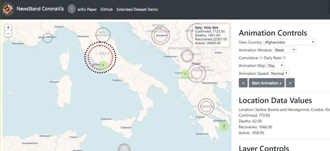
Figure 1: Example NewsStand CoronaViz screenshot for Italy and the Balkan States

Our application is implemented as an interactive website using HTML, CSS, and JavaScript that communicates with our database through a Ruby On Rails web server. It consists of an interactive map query interface that is used to display our data and animations. In addition, a collection of controls are used to download data from our server and to select how it is displayed on the map. A screenshot of our application is shown in Figure NewsStand CoronaViz: A Map Query Interface for Spatio-Temporal and Spatio-Textual Monitoring of Disease Spread, and a more detailed screenshot showing the full control panel is in Figure 2. A second screenshot showing CoronaViz used to visualize data on smaller scale (Italy and the Balkan States) is shown in Figure 1.

4.1 Map Query Interface

Our map query interface is built around an interactive web map provided by the Leaflet JavaScript Library. Data is rendered onto this map using a technique called marker clustering, which is implemented by an extension to Leaflet. Marker clustering allows large numbers of points to be rendered quickly without overloading the user with information. Rather than rendering each point individually, points are clustered into aggregate markers. As the user increases the zoom level of the map, focusing on a smaller area, these aggregate markers are split into two or more new markers that together represent all the points represented by the original marker. This decomposition allows more detail to be displayed when examining a small area without showing too much detail at lower zoom levels.

The interface can display five different data layers: news keywords, twitter keywords, confirmed COVID-19 cases, deaths from COVID-19, and recovered COVID-19 cases. Data for the news and twitter layers was collected as described in Section 3 while data used for the remaining layers was originally gathered by Dong et al. [3]. Layers can be viewed individually or simultaneously to visualize the spatial and temporal relationship between the variables in each layer.

Each marker represents some collection of points, so the size and color of the markers are scaled to represent the magnitude of this collection. Markers representing a single point are set to have a radius of $40$ pixels. From there, the marker’s radius scales with the squared logarithm of the number of points ( $r_{M}=40+\log^{2}2\lvert M\rvert$). Markers for the news data layer also have their color scaled depending on the number points. Green is used for markers representing up to ten points, yellow is used for those that represent up to $100$ points, and red is used for all larger markers. These functions are chosen to be visually appealing, but there is no other concrete reason for their selection.

The map query interface also gives access to the underlying data for each layer. When the user hovers their mouse over a marker, an overlay on the interface is updated to show the exact data values for that marker or marker cluster. When a marker is clicked, this data is also displayed in a in a secondary information box located directly below the animation controls on the right side of our application. This placement is intended to facilitate monitoring changes in data values as the user manipulates the incremental animation controls described in the next section.

4.2 Interface Controls

Figure 2: Screenshot showing the full contents of the controls panel.

The first control located below the map interface is a slider bar that can be manipulated to control the range of dates in the data displayed on the map. Moving either knob on the slider causes the map interface to be updated. The exact dates selected are displayed below the slider. Below the date range slider there are three panels labeled ”Download Controls,” ”Animation Controls,” and ”Layer Controls.”

The download controls are used to retrieve data from our database. First, there is a text entry box labeled “keyword” in which the user types a keyword that they want to visualize. There are then two date entry fields labeled “Data Start Date” and “Data End Date”. These control the range of dates for data that is downloaded from our server. Note that this is not necessarily the same as the range of dates for data that is rendered on the map. Finally, there is a button labeled “Download Data” that, when clicked, sends a request to our server for data within the specified time range matching the provided keyword. This data is rendered on the map query interface, replacing any previous data.

The animation controls deal with using downloaded data to generate time series animations. Most prominently, there is the “Start Animation” button that initiates the animation when clicked. Clicking this button a second time will pause an ongoing animation such that it can be resumed from the current position later. Located to the left and right of this button are two arrow buttons that are used to move incrementally through the animation. Clicking on the left arrow steps backwards to the previous frame of the animation while right arrow advances to the next frame. With the incremental controls, the user can examine the exact data value for each frame of the animation, enabling more precise analysis than would be possible only using the continuous animation mode.

The properties of the animation are controlled by the next four inputs. The first input controls the size of the range of dates displayed in each frame of the animation. It can be set to hour, day, week, or month. It can also be set to a custom size through use of the “Displayed Data Range” controls discussed above. The checkbox below this is used to toggle the cumulative animation mode. Under the default configuration, only an interval defined by the animation window is displayed at one time. This behavior is desirable for monitoring disease spread because it captures where the disease is active at any given time and not every location that it has ever been active. Nonetheless, it may be interesting to view disease spread in a cumulative manner, so this functionality is provided. Next, there is a selection input for the interval advanced between each frame of the animation. This can be set to day, week, or month. The final input field is used to set the speed of the animation to either ”slow”, ”normal”, or ”fast”. These values correspond to a minimum number of milliseconds waited between frames of the animation: $500$, $100$, and $0$ milliseconds respectively. While these are minimum delays, the actual interval may be longer due to time required to compute the subsequent frame.

Finally, the layer controls are used to select between the possible data layers that can be rendered on the map interface. By default, only the news keyword and confirmed cases data layers are selected. Selecting any of the other layers will cause that layer to be rendered in addition to any previously selected layers.

When the confirmed cases layer is selected, there are markers representing the total number of confirmed cases in a location rendered on the map. Similarly there are layers for recoveries and deaths that contain markers representing these variables. When multiple of these layers are selected simultaneously, all selected layers are rendered simultaneously as sets of concentric circles. The concentric circles allow for the comparison of values for different layers in a single location by examining the relative size of circles centered at that location while also allowing for comparison between different locations.

4.3 Example Usage

This subsection provides a walk through demonstrating how our application can be used to obtain an animation to show the geographic change in the discussion of COVID-19 in news articles over time. The instructions here are applicable to other similar uses of our application.

To begin, navigate to coronaviz.umiacs.io to access our website. Once there the “Keyword” entry field should be initially populated with “coronavirus”. If this is not the case, select the field and type in this term. The next step is selecting the range of dates to be viewed. A reasonable range for visualizing Corona Virus might start in December 2019 and proceed until the current date. To make this selection, click on and select a date for the “Data Start Date” field. “Data End Date” should have been initialized the current date, but, if it is not, a date should also be selected here. If the default query term and date range have not been changed, the data should have been retrieved automatically upon loading the webpage; otherwise, the “Download Data” button must be clicked after selecting the custom query term and data range to download this data from our server. This may take a noticeable amount of time depending on network speed and the size of the query result. Once the download is complete, data will be rendered on the map.

The next step is to configure the animations controls and initiate an animation sequence. The animation options (“Animation Window” and “Animation Step”) are set to week and day respectively by default. These should be reasonable values but, at this point, they can be changed. Clicking the “Start Animation” button starts an animation on the map query interface that begins by displaying downloaded data with the earliest publication date and proceeds until the final frame that contains the most recent data. Each frame of the animation shows a period of time defined by “Animation Window” and the start of the frame is advanced by an interval defined by “Animation Step” between each frame. The animation can be terminated early by clicking the button, now labeled “Pause Animation”, a second time.

5 Evaluation

In this section we evaluate the effectiveness of tracking keyword usage in news articles and tweets to better understand the progression of COVID-19. To do this we search for correlation between the confirmed case numbers collected by [3] and the cumulative number of news articles or tweets recognized by our system. We include geographic information in our analysis by limiting it to confirmed cases and news articles in a specific location. We are able to restrict the analysis in this manner because the dataset of confirmed cases we use already organizes confirmed case numbers by location, our news article dataset is geocoded as described in Section 3.1.2, and the Tweet dataset is derived from geotagged tweets. To further investigate the utility of our technique, we perform the comparison at three geographic scales: world, nation, and region. The results of our evaluations are summarized in Table 1 and Figures 3, 4, and 5.

5.1 News Keywords

	Correlation coefficient
Query Area	Keyword coronavirus	No filter
World	$0.75$	$-0.15$
China	$-0.11$	$-0.05$
Hubei Province	$-0.12$	$-0.08$
United States	$0.37$	$-0.11$
Washington state	$0.25$	$0.14$

Table 1: Correlation coefficient between cumulative new articles and confirmed cases at each scale.

(a) World filtered

(b) World unfiltered

Figure 3: Filtered and unfiltered data at the global scale.

We first ignore specific geographic information extracted from articles and perform this analysis on a global scale. This does not utilize the geographic information we collect, but it is interesting as a point of comparison to other scales. Figure 3(a) plots the daily number of articles using the keyword “coronavirus” as a time series between January 22, 2020 and March 20, 2020. To demonstrate the utility of news articles in tracking the progress of the virus, this figure also shows a time series for the daily number of new confirmed cases world wide. It is clear that both datasets trend upwards at similar rates. To determine if correlation exists between article counts and case numbers, we calculated the Pearson correlation coefficient between the datasets. We found the coefficient to be $0.75$, indicating that the datasets are linearly correlated. To investigate the effect of our keyword filter, we performed a similar comparison where we do not filter news articles for any specific terms. Figure 3(b) shows the time series plot for this data. This time, the article counts clearly do not correlate with case numbers. This is realized in a $-0.15$ correlation coefficient. Since the magnitude of the correlation coefficient is significantly larger when applying the keyword filter, we can see that it is useful in this application.

(a) China filtered

(b) China unfiltered

(c) Hubei filtered

(d) Hubei unfiltered

Figure 4: Filtered and unfiltered data in all of China and Hubei province.

The plots in Figure 4 are formatted the same as Figure 3, but they focus on smaller geographic scales. In Figure 4(a), the plot is restricted to articles geocoded to China and confirmed cases in China. The correlation coefficient between these datasets is $-0.11$, indicating that there is no correlation after applying these geographic filters. Figure 4(c) further restricts the data to the Hubei province of China. The correlation coefficient at this scale is $-0.12$, similar to found for all of China. Figures 4(b), and 4(d) show the plots for China and Hubei when the keyword filter is not applied. Since there was no correlation found with the filter applied we do not expect anything to change when it is removed. As expected, the new correlation coefficients are almost unchanged with $-0.05$ and $-0.08$ for China and Hubei respectively.

(a) United States filtered

(b) United States unfiltered

(c) Washington filtered

(d) Washington unfiltered

Figure 5: Filtered and unfiltered data in all of the United States and Washington state.

In our final set of evaluations, we shift geographic focus from China to the United States. Figure 5 contains plots for a country level of China analysis of the United States and a more specific analysis of Washington state. In contrast to the country level analysis where no correlation was found, the correlation coefficient found for the United States ($0.37$) is greater than that found in the global analysis. While the correlation coefficient calculated for the Washington data is much lower ($0.25$), it is notably higher than the values computed for either China or Hubei. The correlation coefficient for the United States and Washington when not applying the keyword filter ($-0.11$ and $0.14$ respectively) is comparable to that for of the three previous datasets.

In our evaluation of the news keyword dataset, we found that the number of news articles using the term ”coronavirus” is correlated with the number of new cases of COVID-19 when correlation is computed at a global scale. When restricting the analysis to a country wide scale, we found weak correlation when using data for the United States, but we were not able to find any correlation in our dataset for China. There is a similar but less pronounced relationship at the region level. While the Washington state dataset does not display particularly strong correlation with the confirmed cases dataset, it is notably higher than the correlation we found for Hubei. A possible explanation for this inconsistency is that many articles discussing COVID-19 will mention China at some point since it is the origin of the virus. To overcome this issue we may be able to develop a technique to determine which term, toponym pairs in a news article should be included in our dataset. Our dataset currently contains an entry for every toponym in an article if the article also contains the query term.

6 Concluding Remarks and Future Work

In this paper we have described the NewsStand CoronaViz system for visualizing spatiotemporal data and its specific application to tracking the progress of the COVID-19 pandemic.

The primary limitation of our current work is in our process for obtaining spatially referenced mentions of COVID-19 from news articles. Our current procedure looks for articles that contain the term ”coronavirus” as a keyword, and then finds all toponyms that are mentioned in the article. While this is good enough to be useful, as demonstrated by the moderate correlation we found, there is room for improvement. In particular, we plan to investigate more sophisticated natural language processing techniques for determining if a given articles discuss the virus and for determining if a specific toponym used in such an article should be counted as a location mentioned in reference to the disease.

We also acknowledge that we have not yet conducted any user study to objectively determine the effectivness of the system. We plan to design and conduct a study of our dynamic concentric proportional symbols and the ability of users to extract information from our system in its animated and incremental modes.

References

- Abdelrazek et al. [2015] A. Abdelrazek, E. Hand, and H. Samet. Brands in NewsStand: Spatio-temporal browsing of business news. In M. Ali, M. Gertz, Y. Huang, M. Renz, and J. Sankaranarayanan, editors, Proceedings of the 23rd ACM SIGSPATIAL International Conference on Advances in Geographic Information Systems, Seattle, WA, Nov. 2015. Article 97.
- Adelfio et al. [2010] M. D. Adelfio, M. D. Lieberman, H. Samet, and K. A. Firozvi. Ontuition: Intuitive data exploration via ontology navigation. In A. El Abbadi, D. Agrawal, M. Mokbel, and P. Zhang, editors, Proceedings of the 18th ACM SIGSPATIAL International Conference on Advances in Geographic Information Systems, pages 540–541, San Jose, CA, Nov. 2010.
- Dong et al. [2020] E. Dong, H. Du, and L. Gardner. An interactive web-based dashboard to track covid-19 in real time. The Lancet Infectious Diseases, 2020.
- Du et al. [2018] Y. Du, L. Ren, Y. Zhou, J. Li, F. Tian, and G. Dai. Banded Choropleth Map. Personal Ubiquitous Computing, 22(3):503–510, June 2018.
- Foley et al. [1990] J. D. Foley, A. van Dam, S. K. Feiner, and J. F. Hughes. Computer Graphics: Principles and Practice. Addison-Wesley, Reading, MA, second edition, 1990.
- Lan et al. [2012] R. Lan, M. D. Lieberman, and H. Samet. The picture of health: map-based, collaborative spatio-temporal disease tracking. In Proceedings of the 1st ACM SIGSPATIAL International Workshop on the Use of GIS in Public Health (HealthGIS 2012), pages 27–35, Redondo Beach, CA, Nov. 2012.
- Lan et al. [2014] R. Lan, M. D. Adelfio, and H. Samet. Spatio-temporal disease tracking using news articles. In Proceedings of the 3rd ACM SIGSPATIAL International Workshop on the Use of GIS in Public Health (HealthGIS 2014), pages 31–38, Dallas, TX, Nov. 2014.
- Li et al. [2019] J. Li, S. Chen, K. Zhang, G. L. Andrienko, and N. V. Andrienko. COPE: interactive exploration of co-occurrence patterns in spatial time series. IEEE Transactions on Visualization and Computer Graphics, 25(8):2554–2567, 2019.
- Lieberman and Samet [2011] M. D. Lieberman and H. Samet. Multifaceted toponym recognition for streaming news. In Proceedings of the 34th International Conference on Research and Development in Information Retrieval (SIGIR’11), pages 843–852, Beijing, China, July 2011.
- Lieberman and Samet [2012] M. D. Lieberman and H. Samet. Adaptive context features for toponym resolution in streaming news. In Proceedings of the 35th International Conference on Research and Development in Information Retrieval (SIGIR’12), pages 731–740, Portland, OR, Aug. 2012.
- Lieberman et al. [2007] M. D. Lieberman, H. Samet, J. Sankaranarayanan, and J. Sperling. STEWARD: architecture of a spatio-textual search engine. In H. Samet, M. Schneider, and C. Shahabi, editors, Proceedings of the 15th ACM International Symposium on Advances in Geographic Information Systems, pages 186–193, Seattle, WA, Nov. 2007.
- Ouyang and Revesz [2000] M. Ouyang and P. Z. Revesz. Algorithms for cartogram animation. In B. C. Desai, Y. Kiyoki, and M. Toyama, editors, 2000 International Database Engineering and Applications Symposium, IDEAS 2000, September 18-20, 2000, Yokohoma, Japan, Proccedings, pages 231–235. IEEE Computer Society, 2000.
- Samet et al. [2014] H. Samet, J. Sankaranarayanan, M. D. Lieberman, M. D. Adelfio, B. C. Fruin, J. M. Lotkowski, D. Panozzo, J. Sperling, and B. E. Teitler. Reading news with maps by exploiting spatial synonyms. Communications of the ACM, 57(10):64–77, Oct. 2014.
- Sankaranarayanan et al. [2009] J. Sankaranarayanan, H. Samet, B. Teitler, M. D. Lieberman, and J. Sperling. TwitterStand: News in tweets. In D. Agrawal, W. G. Aref, C.-T. Lu, M. F. Mokbel, P. Scheuermann, C. Shahabi, and O. Wolfson, editors, Proceedings of the 17th ACM SIGSPATIAL International Conference on Advances in Geographic Information Systems, pages 42–51, Seattle, WA, Nov. 2009.
- Slocum et al. [2009] T. A. Slocum, R. B. McMaster, F. C. Kessler, and H. H. Howard. Thematic Cartography and Geovisualization. Prentice Hall series in geographic information science. Pearson Prentice Hall, Upper Saddle River, NJ, 3rd ed. edition, 2009.
- Teitler et al. [2008] B. Teitler, M. D. Lieberman, D. Panozzo, J. Sankaranarayanan, H. Samet, and J. Sperling. NewsStand: A new view on news. In W. G. Aref, M. F. Mokbel, H. Samet, M. Schneider, C. Shahabi, and O. Wolfson, editors, Proceedings of the 16th ACM SIGSPATIAL International Conference on Advances in Geographic Information Systems, pages 144–153, Irvine, CA, Nov. 2008.
- Wajid and Samet [2016] F. Wajid and H. Samet. CrimeStand: Spatial tracking of criminal activity. In M. Ali, S. Newsam, S. Ravada, M. Renz, and G. Trajcevski, editors, Proceedings of the 24th ACM SIGSPATIAL International Conference on Advances in Geographic Information Systems, Burlingame, CA, Nov. 2016. Article 81.